Coupling Process-Based Models and Machine Learning Algorithms for Predicting Yield and Evapotranspiration of Maize in Arid Environments

Abstract

Crop yield prediction is critical for investigating the yield gap and potential adaptations to environmental and management factors in arid regions. Crop models (CMs) are powerful tools for predicting yield and water use, but they still have some limitations and uncertainties; therefore, combining them with machine learning algorithms (MLs) could improve predictions and reduce uncertainty. To that end, the DSSAT-CERES-maize model was calibrated in one location and validated in others across Egypt with varying agro-climatic zones. Following that, the dynamic model (CERES-Maize) was used for long-term simulation (1990–2020) of maize grain yield (GY) and evapotranspiration (ET) under a wide range of management and environmental factors. Detailed outputs from three growing seasons of field experiments in Egypt, as well as CERES-maize outputs, were used to train and test six machine learning algorithms (linear regression, ridge regression, lasso regression, K-nearest neighbors, random forest, and XGBoost), resulting in more than 1.5 million simulated yield and evapotranspiration scenarios. Seven warming years (i.e., 1991, 1998, 2002, 2005, 2010, 2013, and 2020) were chosen from a 31-year dataset to test MLs, while the remaining 23 years were used to train the models. The Ensemble model (super learner) and XGBoost outperform other models in predicting GY and ET for maize, as evidenced by R² values greater than 0.82 and RRMSE less than 9%. The broad range of management practices, when averaged across all locations and 31 years of simulation, not only reduced the hazard impact of environmental factors but also increased GY and reduced ET. Moving beyond prediction and interpreting the outputs from Lasso and XGBoost, and using global and local SHAP values, we found that the most important features for predicting GY and ET are maximum temperatures, minimum temperature, available water content, soil organic carbon, irrigation, cultivars, soil texture, solar radiation, and planting date. Determining the most important features is critical for assisting farmers and agronomists in prioritizing such features over other factors in order to increase yield and resource efficiency values. The combination of CMs and ML algorithms is a powerful tool for predicting yield and water use in arid regions, which are particularly vulnerable to climate change and water scarcity.

1. Introduction

Maize is the world’s third most important staple food crop, after rice and wheat [1]. In comparison to rice and wheat, maize has a lower protein content but a higher energy density, with 72% carbohydrate and 10% protein, as well as important minerals such as calcium and iron, making it crucial for food security and nutrition [2].

The gap between food consumption and production has grown as a result of limited water resources [3,4], climate change [5], rapid population growth [6], and global crises such as pandemics and wars [7], particularly in water-scarce environments. This requires a lot of attention to improve yield production and close the yield gap. One of the most important environmental abiotic stresses that negatively impact the growth and final yield of many crops is drought stress [8,9]. Determining evapotranspiration is therefore essential to better manage irrigation water and avoid the detrimental impacts of drought stress on plants in order to increase productivity and economic gains of the water–food nexus [10,11]. The ET estimation models available in the literature may be broadly classified as (1) fully physically based combination models that account for mass and energy conservation principles; (2) semi-physically based models that deal with either mass or energy conservation; and (3) black-box models based on artificial neural networks, empirical relationships, and fuzzy and genetic algorithms [12,13,14]. Furthermore, different computing approaches for monitoring and protecting water resources, such as satellite-based data [15], a new front detection algorithm (GRADHIST) [16], and soft computing [17], were considered in the literature. To predict yield and water use, various methods were used, including remote sensing [18,19] and crop models [20,21].

Integration between environmental factors (i.e., soil types, temperatures, carbon dioxide concentrations (CO₂), solar radiation, and available water content) and management practices such as tillage, organic matter, irrigation, and cultivars, can be considered as an integrated approach to enhance maize yield and water productivity, but still has less attention so far due to its difficulty in application to typical field studies due to the large number of factors across spatiotemporal scales. Crop models (CMs) offer the opportunity to address such challenges by combining multiple factors [22,23] following the proper testing against observational data. Many crop models were used to predict crop yield and water use around the world [24], but the Decision Support System for Agro-technology Transfer (DSSAT) is one of the most widely used crop models for adaptation and mitigation development and ultimately supports decision making [25,26]. The CERES-Maize module is one of the most widely used models in the DSSAT model for predicting maize yield and water use [27,28]. However, in arid environments, deploying CERES-Maize to predict maize yield and water use in response to factorial combinations of environmental factors and management practices has received less attention, demonstrating the importance and novelty of current research. Nevertheless, CMs have significant limitations when it comes to making predictions, such as yield-limiting soil nutrients, physical limits in the soil, and different pests, diseases, weeds, and other stresses that reduce production in farmers’ fields but are not currently taken into account in models [29,30]. The various soil and crop processes and how they interact with the environment are approximated by imperfect crop models used in impact assessment studies. The predictive power of these models is frequently limited by large uncertainties related to model structure, choices of model inputs, and parameter values, which exceed the spatiotemporal variability of observed yields [31,32]. This emphasizes the requirement for the development of more effective methods to identify the most significant sources of uncertainty and their underlying causes in order to raise the caliber and transparency of upcoming impact assessments [33]. On the other hand, machine learning algorithms (MLs) could create simulations by creating connections between the inputs of agricultural production elements (such as soil, weather, agronomic methods, and environmental effects) and the projected variables such as crop output [34]. The algorithm “learns” a transfer function from the inputs in MLs, in contrast with CMs, in order to estimate the intended output [35]. Recent research has shown that ML can be used to estimate ET in a variety of terrestrial ecosystems [36,37]. However, few studies have been conducted to estimate ET using a hybrid crop model–ML approach. Because it considers CMs restrictions, MLs offers certain advantages over CMs while having lengthier runtimes defined by the quantity of variables/data we input [38]. Therefore, we combine CMs with different ML algorithms to create a hybrid approach with robust predictions and less uncertainty. Recently, there are different ML algorithms used in crop yield predictions including random forest, support vector machine [39], linear regression, LASSO regression, extreme gradient boosting (XGBoost), LightGBM [40], and convolutional neural networks (CNN) [41]. Nonetheless, such studies used only ML algorithms without coupling them with crop models, as well as using simple treatments of management practices, confirming the significance of our study which combined CMs with multiple ML algorithms under a broad range of environmental factors and management practices. In addition to the base ML models, we developed a super learner (SL) that stacks the base models for higher accuracy and precision. The SL is based on optimality theory, which ensures that for large sample sizes, the SL will perform as well as possible given the specified algorithms [42]. It is an ensemble method that allows researchers to combine multiple prediction algorithms into a single one [43]. Permutation feature importance is a technique that can be used to minimize bias in biological investigations where independent variables may comprise numerical and categorical features [44]. Coupling crop models with ML algorithms in prediction has been used in some recent studies, but most of them ignored using a multimodel approach and only used the default method in testing the models for limited treatments rather than G × M × E interactions. Meanwhile, in the current study, we used MME to predict yield and water use after testing the models with the warmest years and taking into account the G × M × E interactions, confirming the work’s novelty.

Therefore, the main objective of this work is to explore the potential of coupling dynamic crop models (CERES-Maize) with machine learning algorithms for robust prediction of maize yield and water use in different environments. The specific objectives to ensure the main aim include (1) validation of CERES maize under different environments, cultivars, and treatments for maize crop; (2) deploying CMs for long-term prediction (1990–2020) of maize yield and water use under a broad range of environmental and management factors; (3) training and testing several ML algorithms using the detailed outputs of CMS long term simulations; and (4) exploring the most important features from different algorithms that achieved accurate prediction of maize yield and water use in different locations.

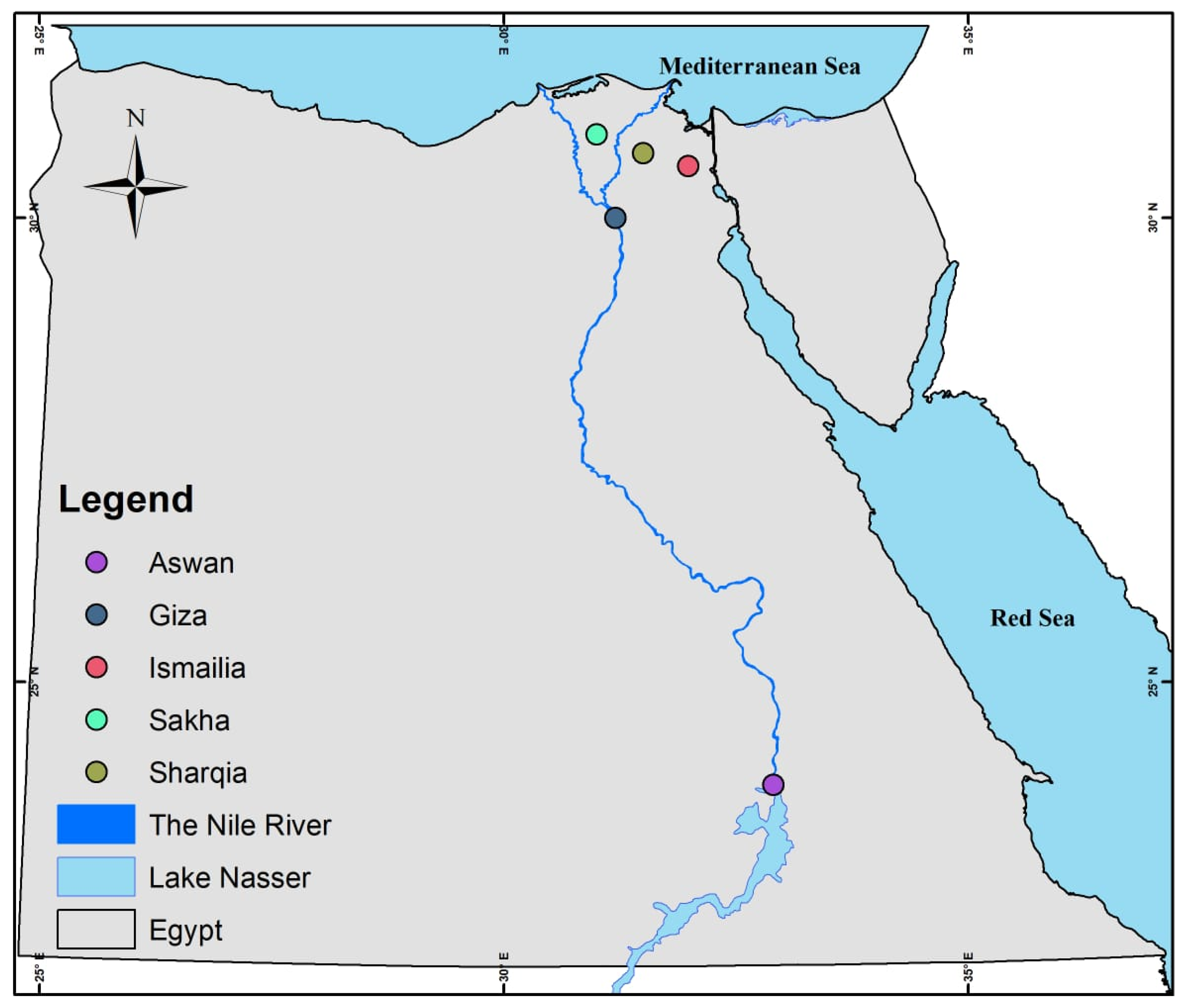
2. Materials and Methods

2.1. Calibration of DSSAT Model

The DSSAT model was calibrated using eight-year site field experiments conducted on arid sandy soil in Ismailia, Egypt [27,45]. Objectives of these experiments were to investigate maize yield and water use in response to several management practices for a total number of treatments of 44 in which all had the final grain yield reported and plant and/or soil measurements (

Table 1. Calibrated values of cultivar-specific parameters for medium-maturity maize variety (CV, SC10) in the DSSAT-CERES-Maize model (v. 4.7.5) for maize experiments in Ismailia, Egypt.

	P1 (C Days)	P2 (Days)	P5 (C Days)	G2 (Number)	G3 (mg day−1)	PHINT (C Days)
Calibration range	130–380	0–2	600–1100	400–1100	4–11.5	35–65
Calibrated values	320	0.8	968	794	8.5	51

P1: Degree days above a base temperature of 8 ℃ from seedling emergence to the end of the juvenile phase; P2: day length sensitivity coefficient that is the delay in days for each hour increase in photoperiod above the longest photoperiod at which development proceeds at maximum rate (12.5 h); P5: degree days above a base temperature of 8 °C from silking to physiological maturity; G2: maximum possible number of kernels plant−1; G3: kernel filling rate during the linear grain filling stage and under optimum conditions (mg day⁻¹); and PHINT: the interval in thermal time (degree days, °C day) between successive leaf tip appearances (Phyllochron interval).

, [27]). Detailed description of these experiments and the calibration procedure are described in Attia et al. [27]. Figure 1 shows the results of phenology and grain yield of maize and soil moisture content and evapotranspiration prediction by the DSSAT model compared with the observed data. The calibrated model was then validated by comparing the phenology and leaf area index of maize as well as the grain and biomass yield prediction at various locations representing different soils and agro-climate zones (Figure 2). The data were extracted from the national maize research program by the Agricultural Research Center (ARC) of Egypt during 2018 to 2020 that included the anthesis and physiological maturity dates, leaf area index, and grain and biomass yields. In this dataset, two maize cultivars were considered: high yield cultivar (SC10) and standard cultivar (TWC324). Supplementary Materials Figure S1 summarizes the story of data collection, modeling, and ML algorithm predictions of yield and water use. The daily climatic parameters such as maximum and minimum temperatures, relative humidity, solar radiation, and wind speed for different locations are presented in the Supplementary Materials, Figure S2.

2.2. Development of the Simulated Dataset

The calibrated model was used to perform a factorial simulation experiment to develop a simulated dataset for ML development and analysis. The factorial combination included two categories: (i) environmental variables and (ii) management variables (

Table 2. Environmental variables and management variables used as input features for model building.

Feature Name	Type	Description	Levels
Environmental variables
Minimum temperature	Numeric	Daily minimum temperature	Baseline, +1, +2, +3, +4
Maximum temperature	Numeric	Daily maximum temperature	Baseline, +1, +2, +3, +4
CO2	Numeric	CO2 concentration	Baseline (380 ppm), +20, +40,+60, +80
Solar radiation	Numeric	Daily solar radiation (MJ/m2/d)	Baseline
Texture	Factor	Soil texture	Sandy, Silty Clay, Silty Clay Loam, and Clay Loam for Ismailia, Giza, Sakha, and Aswan sites, respectively
Available water content	Numeric	Average soil water holding capacity (mm of water/m of soil depth)	65, 115, 145, and 120 for Ismailia, Giza, Sakha, and Aswan sites, respectively
Soil organic carbon	Numeric	Percent of soil organic carbon in 60 cm soil depth	0.46, 0.98, 1.54, and 1.34 for Ismailia, Giza, Sakha, and Aswan sites, respectively
Management variables
Cultivar	Numeric	Calibrated radiation use efficiency	Baseline (3.7), 4.07, 4.44
DOY	Numeric	Day of year	Weakly planting for 3 weeks before the recommended planting date and 3 weeks after the recommended planting date, plus the recommended planting date totaling 7 planting dates
Irrigation *	Numeric	Percent of available soil moisture content in the 30 cm soil depth	90%, 70%, 50%, and 30%
Compost	Numeric	Level of compost application	0, 5000 kg/ha and 10,000 kg/ha
Tillage	Factor	Tillage operation	No tillage and conventional tillage

* Irrigation factor justified to be triggered at different levels of depletion from available water.

). The environmental variables included minimum and maximum temperature, solar radiation, CO₂ concentration, soil type (texture), soil available water content, and soil organic matter. Within the temperature and CO₂ concentration, there were five levels of the baseline plus four increment levels, whereas the solar radiation included the baseline level only. Other environmental variables were related to the four sites that were used in the study, each of which had soil type, available water content, and organic matter content. For instance, at the Ismailia site the soil texture is sandy, the available water content is 65 mm/m, and the soil organic carbon is 0.46 (Table 2). The management variables included: radiation use efficiency (cultivar) calibrated value plus two other levels; planting date (DOY); recommended planting date plus and minus 3 weeks from the recommended date; four irrigation levels according to the percent of soil moisture depletion; compost application with three levels; and tillage operation represented by no-till and conventional tillage. The recommended planting date is 15 May at Ismailia, Sakha, and Giza and 25 July at Aswan. The combination of 29 factorial levels (temperature, CO₂ concentration, solar radiation, cultivar, DOY, irrigation, compost, and tillage) in four sites for 31 years (1990–2020) resulted in more than 1.5 million simulated scenarios of yield and evapotranspiration. Each scenario represented an instance of a full factorial design; therefore, all possible scenarios were simulated. R software v. 4.1.2 [46] was utilized to facilitate editing of the “File X” and run the model for the factorial levels each year of the long term simulation using the DSSAT package (https://cran.r-project.org/web/packages/DSSAT/index.html (accessed on 1 March 2022)). The simulation profile started two weeks ahead of the first planting date of the corresponding site and was run independently for 31 years, i.e., resetting to the initial condition each year.

2.3. Machine Learning Models Development and Testing

Six machine learning models were developed to predict maize yield and evapotranspiration that included three types of linear regression (linear, ridge, and lasso), and three tree-based methods (K-nearest neighbors, random forest, and extreme gradient boosting (XGBoost)) using the scikit-learn machine learning package in Python (https://scikit-learn.org/stable/, accessed 1 March 2022). The dataset was partitioned to training and testing data, while data from the selected years (1991, 1998, 2002, 2005, 2010, 2013, and 2020) were used as the testing dataset (23%), whereas the remaining dataset was used as training dataset (77%). The tested years were selected based on their higher content of temperatures compared with other years. Hyperparameters tuning was performed to optimize the models’ prediction of maize grain yield and evapotranspiration utilizing the Hyperopt package in Python [30]. The Hyperopt employs a Bayesian approach to find the best values of the hyperparameters over the specified parameters’ space. The objective function aimed at minimizing the root mean square error between the testing data and the fitted model prediction. This process was performed to find the best values of the hyperparameters for all models except the multiple linear regression as a baseline for comparison (

Table 3. Hyperparameters space and optimized values for several machine learning models.

Model	Hyperparameter	Space	Optimized Values for Grain Yield	Optimized Values for Evapotranspiration
Ridge regression	‘alpha’	‘alpha’: (0,10000)	‘alpha’: 51.603	‘alpha’: 3.326
Lasso regression	‘alpha’	‘alpha’: (0,10000)	‘alpha’: 0.011	‘alpha’: 0.044
K-nearest neighbors	{‘leaf_size’, ‘n_neighbors’}	{‘leaf_size’: (1,50), ‘n_neighbors’: (1,30)}	{‘leaf_size’: 47, ‘n_neighbors’: 22}	{‘leaf_size’: 11, ‘n_neighbors’: 20}
Random forest	{‘max_depth’, ‘min_samples_leaf’, ‘min_samples_split’, ‘n_estimators’}	{‘max_depth’: (5,20), ‘min_samples_leaf’: (1,5), ‘min_samples_split’: (2,6), ‘n_estimators’: (100,500)}	{‘max_depth’: 9.874, ‘min_samples_leaf’: 4.584, ‘min_samples_split’: 4.145, ‘n_estimators’: 485.329}	{‘max_depth’: 9.087, ‘min_samples_leaf’: 1.971, ‘min_samples_split’: 5.769, ‘n_estimators’: 265.092}
XGBoost	{‘colsample_bytree’, ‘gamma’, ‘max_depth’, ‘min_child_weight’, ‘n_estimators’, ‘reg_alpha’, ‘reg_lambda’}	{‘colsample_bytree’: (0.5,1), ‘gamma’: (1,9), ‘max_depth’: (3,18), ‘min_child_weight’: (0,10), ‘n_estimators’: (80,280), ‘reg_alpha’: (40,180), ‘reg_lambda’: (0,1)}	{‘colsample_bytree’: 0.803, ‘gamma’: 2.01, ‘max_depth’: 3.0, ‘min_child_weight’: 7.0, ‘n_estimators’: 14, ‘reg_alpha’: 53.0, ‘reg_lambda’: 0.432}	{‘colsample_bytree’: 0.562, ‘gamma’: 5.565, ‘max_depth’: 3.0, ‘min_child_weight’: 10.0, ‘n_estimators’: 63, ‘reg_alpha’: 162.0, ‘reg_lambda’: 0.816}

). Following the base model’s optimization, a super learner ensemble was developed by stacking the optimized base models using out-of-fold predictions for base models collected during the k-fold cross-validation. Model performance was evaluated using three statistical indicators of root mean square error (RMSE), relative RMSE (R-RMSE), and coefficient of determination (R²) [31]. Interpretation of relative RMSE indicates that an R-RMSE value < 10% means an “excellent” prediction, >10% and <20% means a “good” prediction, >20% and <30% means a “fair” prediction, and >30% means a “poor” prediction.

2.4. Feature Importance and Meta-Model Comparison with DSSAT Model

Feature importance for Lasso model as an example of linear regression models and for XGBoost as an example of tree-based models was estimated using Tree Explainer by the shape package in Python (https://shap.readthedocs.io/en/latest/index.html, accessed 1 March 2022) [32]) to identify the strongest predictors. The Tree Explainer method uses Shapley values to illustrate the global importance of features and their ranking as well as the local impact of each feature on the model output. The analysis was performed on the model prediction of a representative sample from the testing dataset. Further evaluation of the models’ predictions was performed by comparing the meta-model’s prediction against the DSSAT model prediction at a fifth independent site located at Sharqia (Figure 2). The weather data for this site were provided to the DSSAT model as well as the soil data which are closely similar to the GIZA site. In order to be consistent with the input features used in the model training, the soil-related environmental variables (texture, OC, and AWC) were taken from the GIZA site. The simulated dataset included two sets: (i) the first set responded to varying the management variables only without modifying the environmental variables and (ii) the second set responded to varying the environmental variables only that included the soil inputs for the other three sites at Ismailia, Sakha, and ASWAN while keeping all management variables constant at the recommended practice (planting date: 15 May at Ismailia, Giza, Sakha, and Sharqia and 25 July at Aswan; irrigation: 90%; cultivar: 3.7%; and tillage: conventional tillage). The grain yield and evapotranspiration of maize were predicted by the super learner model given the input features provided to the DSSAT model. The outputs of the super learner model and the DSSAT model were compared and graphed.

3. Results and Discussion

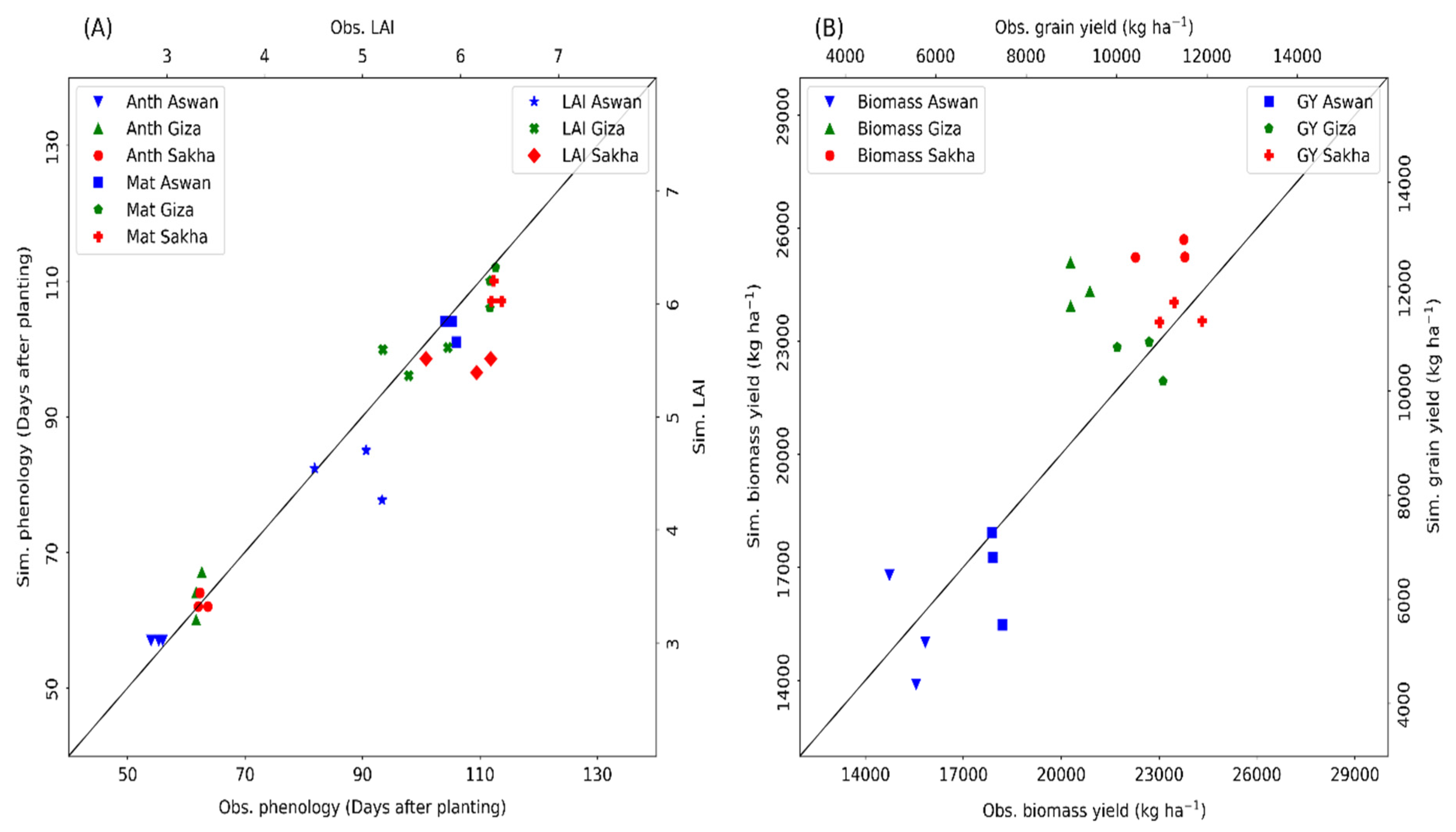
3.1. Validation of DSSAT Maize Model

The calibrated model was then validated using different datasets of maize phenology and yield in different locations varied from lower temperature in Sakha located at the North Nile delta, to moderate temperature in Giza, and higher temperature in Aswan in south Egypt (Figure 2 and Figure 3). The validation results showed a good agreement between observed and simulated phenology, LAI (Figure 3A), biomass yield, and grain yield (Figure 3B). The findings of these features were confirmed by different statistical indicators such as RMSE, normalized root mean square error (nRMSE), and mean percentage error (MPE) (Supplementary Materials, Table S1). These indicators showed lower values for phenology, grain yield, biomass, and non-stressed irrigation treatment (I1), while there was little increase in these indicators with LAI and stressed irrigation treatment (I2). This confirms the high accuracy of model calibration and the potential of using CERES-Maize in long-term simulation even in different locations. Pasquel et al. [47] found that using only RMSE is not enough to evaluate the models, while multi indicators can be considered, confirming the importance of using different statistical indicators in our study. Some features showed little overestimation or underestimation due to some uncertainties in the warmest location and the second cultivar (TWC324) which is considered more sensitive to higher temperatures than SC10 [18]. Nevertheless, both cultivars share a similar genetic background with closely similar yield potential.

3.2. Evaluation of Trained ML Algorithms

In general, the tested ML algorithms predicted maize grain yield and water use with greater accuracy, as indicated by R² > 75% and RRMSE < 10% (

Table 4. Evaluation metrics for various machine learning algorithms built to predict maize yield and evapotranspiration for the testing dataset (1991, 1998, 2002, 2005, 2010, 2013, and 2020).

	RMSE (kg ha−1)	R-RMSE (%)	R2	RMSE	R-RMSE	R2
	Grain Yield (kg ha−1)			Evapotranspiration (mm)
Linear regression	1467	9.76	0.77	64	7.23	0.79
Ridge regression	1468	9.77	0.77	64	7.24	0.80
Lasso regression	1467	9.76	0.77	64	7.23	0.79
K-nearest neighbors	1287	8.56	0.82	36	4.12	0.93
Random forest	1296	8.62	0.82	39	4.44	0.92
XGBoost	1285	8.55	0.82	37	4.27	0.93
Super learner model	1185	7.88	0.85	35	4.03	0.94

). Meanwhile, comparison among the base models showed that the tree-based ML XGBoost model excelled others. Therefore, it was selected to perform feature importance analysis in addition to the lasso regression as the baseline model. These findings were consistent with [38,48]’s findings that XGBoost outperformed other ML algorithms in yield predictions. Interestingly, the SL model achieved the highest accuracy compared with others which can be attributed to the rapid development of soft computing; ensemble models can produce more accurate predictions than a single machine learning model [33].

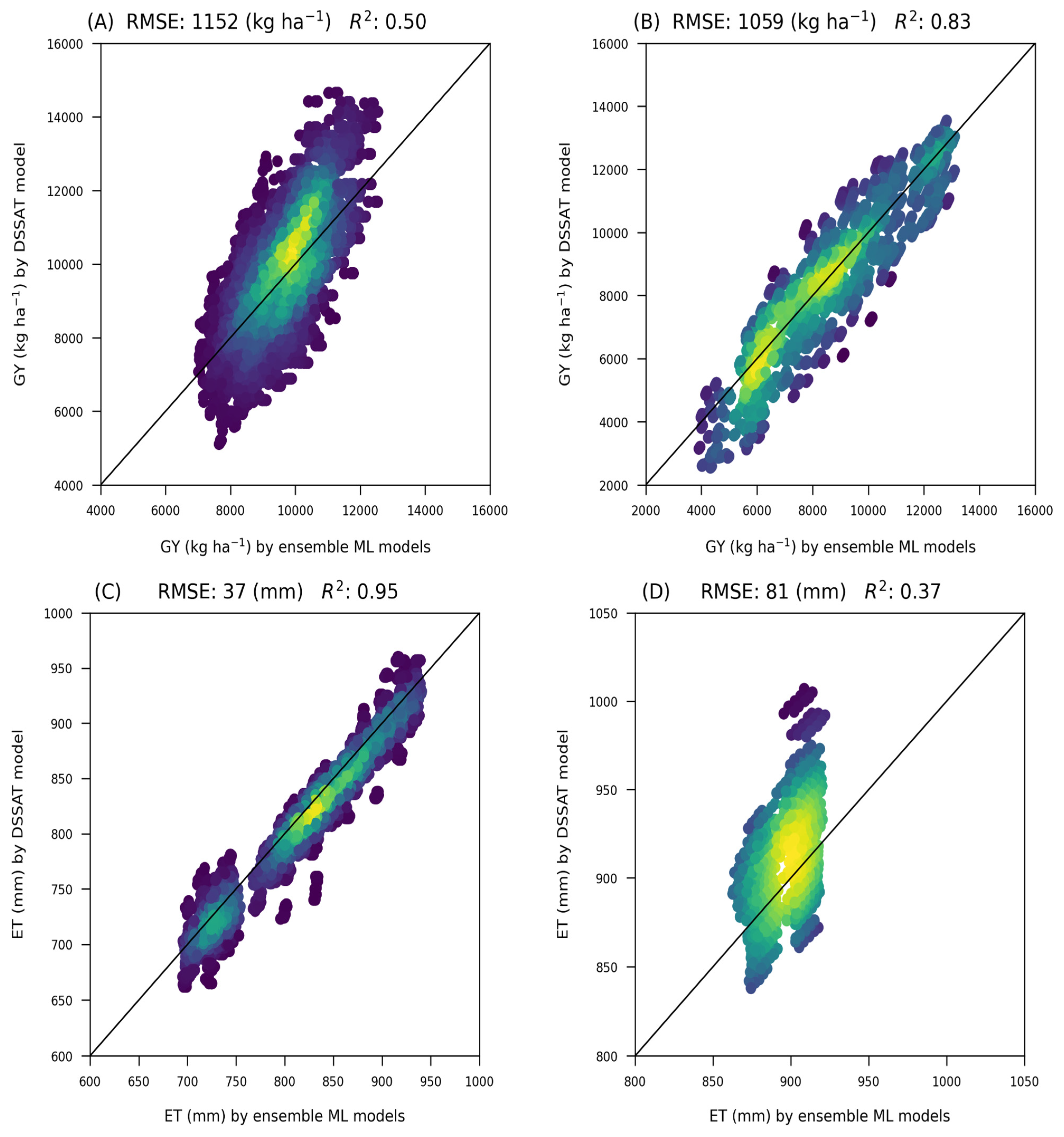
3.3. Predicted Grain Yield and Water Use by DSSAT and ML Algorithms under Broad Range of Management and Environmental Practices

Predicted maize grain yield and water use by DSSAT and ML algorithms differed in response to changing the management and environmental variables, indicating good agreements between DSSAT and ML predictions (Figure 4). We changed the management variables (cultivar, sowing window, irrigation, compost, and tillage) while keeping the environmental factors constant for each feature of GY and ET (Figure 4A,C) at a fifth independent location in Sharqia (Figure 2). Then, while keeping management constant, changed the environmental factors (such as maximum and minimum temperatures, CO₂, solar radiation, soil texture, AWC, and SOC) (Figure 4B,D) by running the model at all locations and therefore varying the soil inputs. Predicted maize grain yield ranged from 7000 to 13,500 kg ha⁻¹ with little variation when management factors were changed (Figure 4A), whereas when environmental factors were changed, GY ranged from 4000 to 13,500 kg ha⁻¹ (Figure 4B). This suggests that environmental factors have a greater impact on maize yield than management practices, but the latter is critical for mitigating the hazard impact caused by environmental variables. This is mainly due to rising temperatures, which shorten crop growth periods and damage cell division and amyloplast replication in maize kernels, resulting in a smaller grain sink and, ultimately, a lower yield [34]. However, changes in different management variables alleviated such reductions and kept the yield ranging from 7000 to 13,500 kg ha⁻¹. Previous research found that technological advancements in genetics, agronomy, and resource use methods account for a sizable share of the improvements in agricultural production [35,36,37]. Nonetheless, due to the difficulty of using a broad range in the field, such studies used a narrow range of management practices. Crop-based models and ML algorithms have the potential to manage a wide range of practices if properly calibrated and trained. This validates the importance of the current study in investigating the effects of environmental variables on maize grain yield, as well as the potential of integrating many management factors as potential adaptations using CMs and MLs algorithms. Prior studies concluded that, model ensembles have been found to be superior yield forecasters in crop and other modeling applications than any single simulation model [38,39,40,41]. We observed the same pattern with ML multi-models in this investigation. In fact, equally weighted ensemble meta-models outperformed single models in terms of yield and evapotranspiration prediction.

Under management practices, the predicted ET by both CMs and ML algorithms were very close to each other (Figure 4C), while DSSAT predicted values were slightly overestimated in the case of environmental changes (Figure 4D). This could be due to the large number of training iterations and parameter tuning in ML, which could result in higher prediction accuracy and less uncertainty. The hyperparameters of a machine learning model must be tuned to fit it to different problems. The best hyperparameter configuration for machine learning models has a direct effect on model performance. It frequently necessitates extensive knowledge of machine learning algorithms and hyperparameter optimization techniques. Although there are several automatic optimization techniques, their strengths and drawbacks differ when applied to different types of problems. According to various studies [49,50], hyperparameter tuning outperforms other optimization methods. Furthermore, ML algorithms use inputs from CM model outputs as well as the original and initial dataset to create a hybrid approach that improves prediction over individual crop models [42]. This confirms that a hybrid approach of CMs and MLs is far superior to using some of them individually for robust yield and water use predictions.

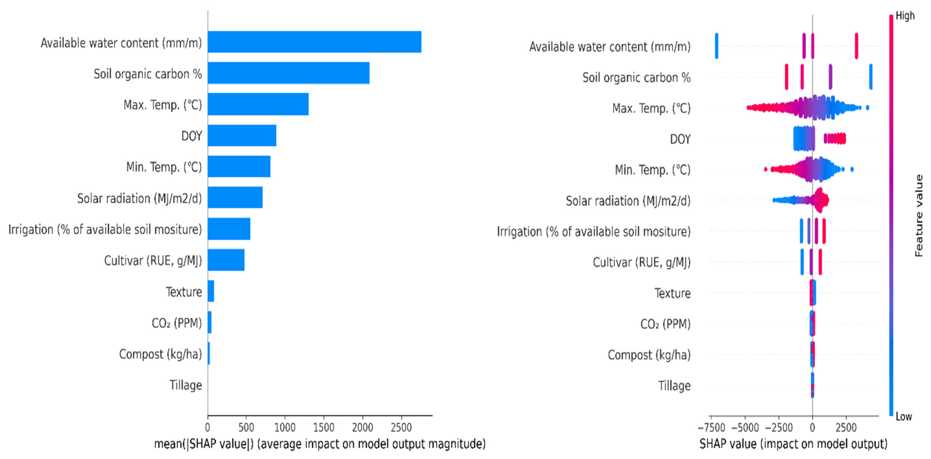
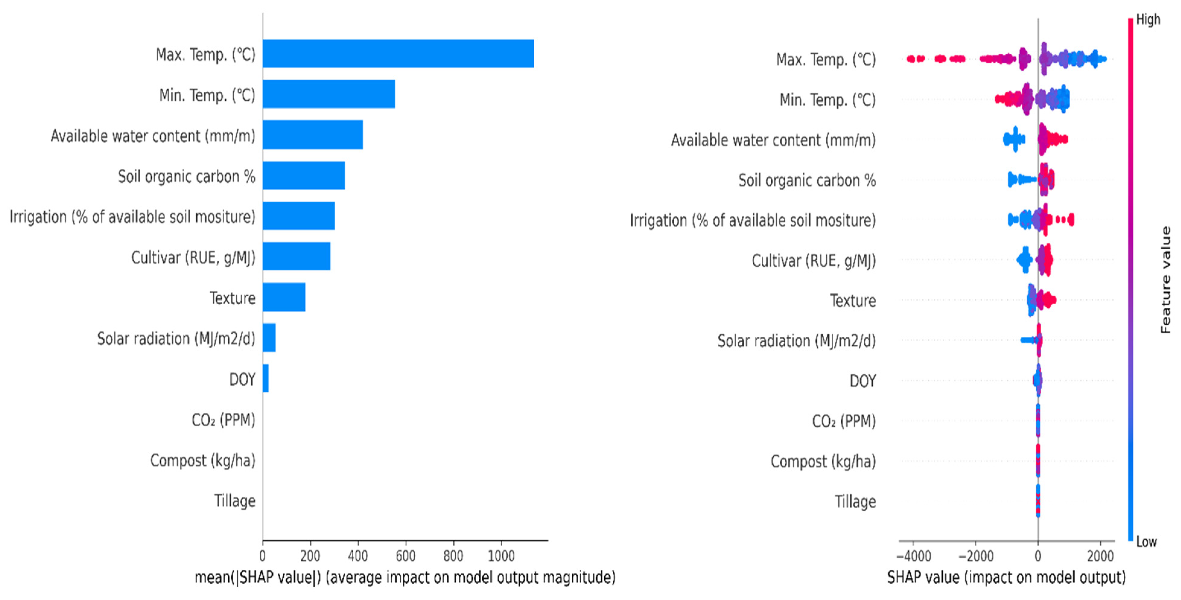
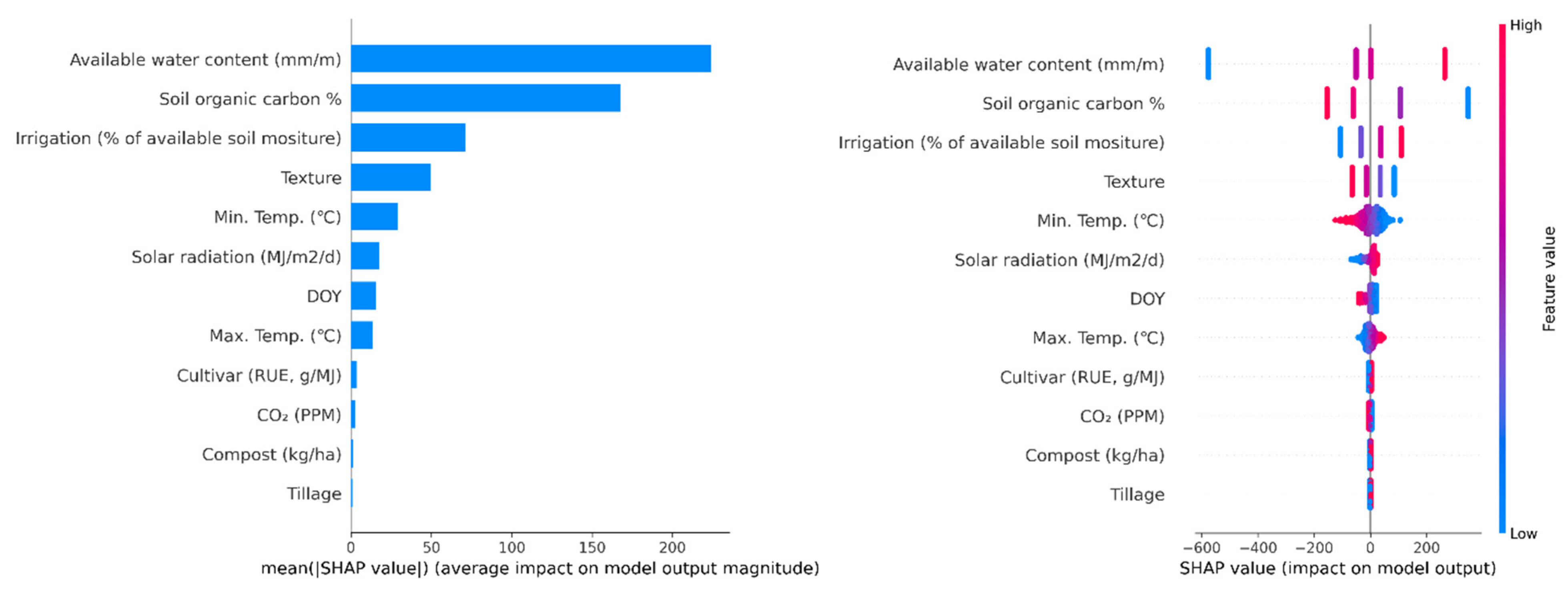
3.4. The Most Important Variables

The important features of predicted GY and ET were presented for lasso regression as a standard model and for XGBoost as the best model (Figure 5, Figure 6, Figure 7 and Figure 8). To investigate the most important features of each proposed model, we predicted maize grain yield and evapotranspiration using different management and environmental variables (Table 2). Determining the most important features is critical to assisting farmers and agronomists in focusing on such features to increase yield and resource efficiency values over other factors [25]. In this case, we used the SHAP method to represent and explain the important features that contribute more to the ML outputs. Features with higher shapely values contribute more to predicted yield and evapotranspiration, while features with lower Shapley values contribute less. To determine the global importance, the average absolute Shapley value per feature across the entire dataset (management and environment) is calculated (Figure 5, Figure 6, Figure 7 and Figure 8, left). Furthermore, the local explanation summary indicates the direction of the relationship between a feature and the model output. Positive SHAP-values indicate increased grain yield or ET, while negative SHAP-values indicate decreased components (Figure 5, Figure 6, Figure 7 and Figure 8, right). Figure 4 depicted the important features of GY predicted by the lasso regression model. Available water content (AWC), soil organic carbon, maximum temperature, planting date (DOY), minimum temperature, solar radiation, irrigation, and cultivar type were the most important factors associated with the predicted GY by the lasso regression model (Figure 4, left). The SHAP-values (Figure 4, right), showed that the features of increasing AWC, delaying planting date, solar radiation, irrigation, resistant cultivar, CO₂, and compost correlated positively with maize grain yield. Meanwhile, rising temperatures significantly reduced the predicted maize grain yield. In the case of yield predictions by the XGBoost model, data showed that the important features could be arranged in the following sequence order: maximum temperature, minimum temperature, AWC, soil organic carbon, irrigation, cultivars, soil texture, solar radiation, and planting date (Figure 6, left). The SHAP-values derived from such features revealed that maximum and minimum temperature correlated negatively with predicted grain yield, whereas other features increased yield with a significant contribution from irrigation. Low temperatures increase growth duration, which allows crops to intercept more radiation, so high corn yield is associated with low temperatures, high solar radiation, and irrigation [43]. We can infer from this analysis that heat-tolerant cultivars (SC10) can be used to lessen yield losses because they can partially offset the effects of high temperatures on leaf area, photosynthetic rate, and growth and development [43].

The lasso regression model predicted ET by twelve features (Figure 7) and XGBoost (Figure 8). The global important features from lasso regression were ordered as AWC > SOC > irrigation > soil texture > minimum temperature > solar radiation > planting date > maximum temperature > cultivar > CO₂ > compost > tillage (Figure 7, left). When compared with other features, increasing the minimum temperature and sowing date reduced the predicted ET (Figure 7, right). Unlike the lasso regression model, the predicted ET by the XGBoost model showed a different order in the important features as irrigation > AWC > soil texture > SOC > planting date > minimum temperature > solar radiation > maximum temperature > cultivar type > CO₂ > compost > tillage (Figure 8, left). Notably, irrigation and other management practices, particularly soil organic carbon and changing planting date, had the greatest impact on crop ET, mitigating the risk impact of environmental factors, particularly temperature (Figure 8, right). Similar findings were observed by [44], who stated that agronomic practice factors such as irrigation, fertilization, and agricultural film contributed positively to the increase in water productivity, while climatic factors such as daily mean temperature and solar radiation contributed less. Taking the most important feature from the best model (XGBoost), it is possible to conclude that temperature was the most important feature for the predicted GY, while irrigation was the most important feature for the predicted ET. Multi-agronomic practices were effectively used as adaptation tools to mitigate the impact of environmental factors.

4. Conclusions

In this paper, we combined the DSSAT CERES maize model with six machine learning models to predict maize grain yield and evapotranspiration in Egypt’s various agroclimatic zones and under a variety of management practices and environmental factors. First, the DSSAT CERES maize model was calibrated for yield, phenology, and evapotranspiration using analogous observed datasets in some locations, followed by validation using data from other locations. The combination of 29 factorial levels (temperature, CO₂ concentration, solar radiation, cultivar, planting date, compost, and tillage) in 4 sites for 31 years (1990–2020) resulted in over 1.5 million yield and evapotranspiration simulated scenarios. The detailed outputs from DSSAT models were used to train and test different Ml algorithms. Following all ML algorithms’ training and testing, the XGBoost model outperformed the other ML regression models in predicting maize grain yield and evapotranspiration, confirmed by higher values of R² and lower RMSE and RRMSE. Despite yield reductions and increased evapotranspiration as temperatures rose, management practices (i.e., irrigation, cultivar changes, sowing date changes, compost, and tillage) mitigated such negative impacts and improved yield and reduced ET. Furthermore, the proposed ML algorithms identified the most important features that significantly contributed to yield and ET predictions, which can assist farmers and decision makers in prioritizing such features over other factors in order to increase yield and resource efficiency values. In arid regions and similar environments, a hybrid approach of CMs-MLs could be used successfully to predict yield and water use under a wide range of management practices and environmental factors. Nonetheless, expanding the current approach to include crop models–machine learning–deep learning as a hybrid under future climate change could be viewed as a prospective ensemble method, particularly in arid and semi-arid environments.

References

1. Gomaa, M.A.; Kandil, E.E.; El-Dein, A.A.M.Z.; Abou-Donia, M.E.M.; Ali, H.M.; Abdelsalam, N.R. Increase maize productivity and water use efficiency through application of potassium silicate under water stress. Sci. Rep. 2021, 11, 224. [Google Scholar] [CrossRef] [PubMed]
2. Ranum, P.; Peña-Rosas, J.P.; Garcia-Casal, M.N. Global maize production, utilization, and consumption. Ann. N. Y. Acad. Sci. 2014, 1312, 105–112. [Google Scholar] [CrossRef]
3. Maroufpoor, S.; Bozorg-Haddad, O.; Maroufpoor, E.; Gerbens-Leenes, P.W.; Loáiciga, H.A.; Savic, D.; Singh, V.P. Optimal virtual water flows for improved food security in water-scarce countries. Sci. Rep. 2021, 11, 21027. [Google Scholar] [CrossRef] [PubMed]
4. McLaughlin, D.; Kinzelbach, W. Food security and sustainable resource management. Water Resour. Res. 2015, 51, 4966–4985. [Google Scholar] [CrossRef]
5. Köberle, A.C. Food security in climate mitigation scenarios. Nat. Food 2022, 3, 98–99. [Google Scholar] [CrossRef]
6. Godfray, H.C.J.; Beddington, J.R.; Crute, I.R.; Haddad, L.; Lawrence, D.; Muir, J.F.; Pretty, J.; Robinson, S.; Thomas, S.M.; Toulmin, C. Food Security: The Challenge of Feeding 9 Billion People. Science 2010, 327, 812–818. [Google Scholar] [CrossRef] [Green Version]
7. Bentley, A.R.; Donovan, J.; Sonder, K.; Baudron, F.; Lewis, J.M.; Voss, R.; Rutsaert, P.; Poole, N.; Kamoun, S.; Saunders, D.G.O.; et al. Near- to long-term measures to stabilize global wheat supplies and food security. Nat. Food 2022, 3, 483–486. [Google Scholar] [CrossRef]
8. Gholami, R.; Zahedi, S.M. Identifying superior drought-tolerant olive genotypes and their biochemical and some physiological responses to various irrigation levels. J. Plant Nutr. 2019, 42, 2057–2069. [Google Scholar] [CrossRef]
9. Çakir, R. Effect of water stress at different development stages on vegetative and reproductive growth of corn. Field Crops Res. 2004, 89, 1–16. [Google Scholar] [CrossRef]
10. Kheir, A.M.S.; Alrajhi, A.A.; Ghoneim, A.M.; Ali, E.F.; Magrashi, A.; Zoghdan, M.G.; Abdelkhalik, S.A.M.; Fahmy, A.E.; Elnashar, A. Modeling deficit irrigation-based evapotranspiration optimizes wheat yield and water productivity in arid regions. Agric. Water Manag. 2021, 256, 107122. [Google Scholar] [CrossRef]
11. Clothier, B.; Jovanovic, N.; Zhang, X. Reporting on water productivity and economic performance at the water-food nexus. Agric. Water Manag. 2020, 237, 106123. [Google Scholar] [CrossRef]
12. Srivastava, A.; Sahoo, B.; Raghuwanshi, N.S.; Chatterjee, C. Modelling the dynamics of evapotranspiration using Variable Infiltration Capacity model and regionally calibrated Hargreaves approach. Irrig. Sci. 2018, 36, 289–300. [Google Scholar] [CrossRef]
13. Sahoo, B.; Walling, I.; Deka, B.C.; Bhatt, B.P. Standardization of Reference Evapotranspiration Models for a Subhumid Valley Rangeland in the Eastern Himalayas. J. Irrig. Drain. Eng. 2012, 138, 880–895. [Google Scholar] [CrossRef]
14. Kumar, U.; Sahoo, B.; Chatterjee, C.; Raghuwanshi, N.S. Evaluation of Simplified Surface Energy Balance Index (S-SEBI) Method for Estimating Actual Evapotranspiration in Kangsabati Reservoir Command Using Landsat 8 Imagery. J. Indian Soc. Remote Sens. 2020, 48, 1421–1432. [Google Scholar] [CrossRef]
15. Lama, G.F.C.; Sadeghifar, T.; Azad, M.T.; Sihag, P.; Kisi, O. On the Indirect Estimation of Wind Wave Heights over the Southern Coasts of Caspian Sea: A Comparative Analysis. Water 2022, 14, 843. [Google Scholar] [CrossRef]
16. Kirches, G.; Paperin, M.; Klein, H.; Brockmann, C.; Stelzer, K. GRADHIST—A method for detection and analysis of oceanic fronts from remote sensing data. Remote Sens. Environ. 2016, 181, 264–280. [Google Scholar] [CrossRef]
17. Sadeghifar, T.; Lama, G.F.C.; Sihag, P.; Bayram, A.; Kisi, O. Wave height predictions in complex sea flows through soft-computing models: Case study of Persian Gulf. Ocean. Eng. 2022, 245, 110467. [Google Scholar] [CrossRef]
18. Hara, P.; Piekutowska, M.; Niedbała, G. Selection of Independent Variables for Crop Yield Prediction Using Artificial Neural Network Models with Remote Sensing Data. Land 2021, 10, 609. [Google Scholar] [CrossRef]
19. Jiang, L.; Yang, Y.; Shang, S. Remote Sensing&mdash;Based Assessment of the Water-Use Efficiency of Maize over a Large, Arid, Regional Irrigation District. Remote Sens. 2022, 14, 2035. [Google Scholar] [CrossRef]
20. Kheir, A.M.S.; Hoogenboom, G.; Ammar, K.A.; Ahmed, M.; Feike, T.; Elnashar, A.; Liu, B.; Ding, Z.; Asseng, S. Minimizing trade-offs between wheat yield and resource-use efficiency in the Nile Delta—A multi-model analysis. Field Crops Res. 2022, 287, 108638. [Google Scholar] [CrossRef]
21. Attia, A.; Rajan, N.; Nair, S.S.; DeLaune, P.B.; Xue, Q.; Ibrahim, A.M.H.; Hays, D.B. Modeling Cotton Lint Yield and Water Use Efficiency Responses to Irrigation Scheduling Using Cotton2K. Agron. J. 2016, 108, 1614–1623. [Google Scholar] [CrossRef]
22. Ding, Z.; Ali, E.F.; Elmahdy, A.M.; Ragab, K.E.; Seleiman, M.F.; Kheir, A.M.S. Modeling the combined impacts of deficit irrigation, rising temperature and compost application on wheat yield and water productivity. Agric. Water Manag. 2021, 244, 106626. [Google Scholar] [CrossRef]
23. Asseng, S.; Jamieson, P.D.; Kimball, B.; Pinter, P.; Sayre, K.; Bowden, J.W.; Howden, S.M. Simulated wheat growth affected by rising temperature, increased water deficit and elevated atmospheric CO2. Field Crops Res. 2004, 85, 85–102. [Google Scholar] [CrossRef]
24. Martre, P.; Wallach, D.; Asseng, S.; Ewert, F.; Jones, J.W.; Rötter, R.P.; Boote, K.J.; Ruane, A.C.; Thorburn, P.J.; Cammarano, D.; et al. Multimodel ensembles of wheat growth: Many models are better than one. Glob. Change Biol. 2015, 21, 911–925. [Google Scholar] [CrossRef] [PubMed]
25. Hoogenboom, G.; Porter, C.H.; Boote, K.J.; Shelia, V.; Wilkens, P.W.; Singh, U.; White, J.W.; Asseng, S.; Lizaso, J.I.; Moreno, L.P.; et al. The DSSAT crop modeling ecosystem. In Advances in Crop Modeling for a Sustainable Agriculture; Boote, K.J., Ed.; Burleigh Dodds Science Publishing: Cambridge, UK, 2019; pp. 173–216. [Google Scholar] [CrossRef]
26. Kothari, K.; Ale, S.; Attia, A.; Rajan, N.; Xue, Q.; Munster, C.L. Potential climate change adaptation strategies for winter wheat production in the Texas High Plains. Agric. Water Manag. 2019, 225, 105764. [Google Scholar] [CrossRef]
27. Attia, A.; El-Hendawy, S.; Al-Suhaibani, N.; Tahir, M.U.; Mubushar, M.; Vianna, M.d.S.; Ullah, H.; Mansour, E.; Datta, A. Sensitivity of the DSSAT model in simulating maize yield and soil carbon dynamics in arid Mediterranean climate: Effect of soil, genotype and crop management. Field Crops Res. 2021, 260, 107981. [Google Scholar] [CrossRef]
28. Ali, M.G.M.; Ahmed, M.; Ibrahim, M.M.; El Baroudy, A.A.; Ali, E.F.; Shokr, M.S.; Aldosari, A.A.; Majrashi, A.; Kheir, A.M.S. Optimizing sowing window, cultivar choice, and plant density to boost maize yield under RCP8.5 climate scenario of CMIP5. Int. J. Biometeorol. 2022, 66, 971–985. [Google Scholar] [CrossRef]
29. Van Ittersum, M.K.; Cassman, K.G.; Grassini, P.; Wolf, J.; Tittonell, P.; Hochman, Z. Yield gap analysis with local to global relevance—A review. Field Crops Res. 2013, 143, 4–17. [Google Scholar] [CrossRef] [Green Version]
30. Gustafson, D.I.; Jones, J.W.; Porter, C.H.; Hyman, G.; Edgerton, M.D.; Gocken, T.; Shryock, J.; Doane, M.; Budreski, K.; Stone, C. Climate adaptation imperatives: Untapped global maize yield opportunities. Int. J. Agric. Sustain. 2014, 12, 471–486. [Google Scholar] [CrossRef]
31. Lama, G.F.C.; Errico, A.; Pasquino, V.; Mirzaei, S.; Preti, F.; Chirico, G.B. Velocity uncertainty quantification based on Riparian vegetation indices in open channels colonized by Phragmites australis. J. Ecohydraulics 2022, 7, 71–76. [Google Scholar] [CrossRef]
32. Khan, M.A.; Sharma, N.; Lama, G.F.C.; Hasan, M.; Garg, R.; Busico, G.; Alharbi, R.S. Three-Dimensional Hole Size (3DHS) Approach for Water Flow Turbulence Analysis over Emerging Sand Bars: Flume-Scale Experiments. Water 2022, 14, 1889. [Google Scholar] [CrossRef]
33. Lobell, D.B.; Asseng, S. Comparing estimates of climate change impacts from process-based and statistical crop models. Environ. Res. Lett. 2017, 12, 015001. [Google Scholar] [CrossRef]
34. Reichstein, M.; Camps-Valls, G.; Stevens, B.; Jung, M.; Denzler, J.; Carvalhais, N.; Prabhat. Deep learning and process understanding for data-driven Earth system science. Nature 2019, 566, 195–204. [Google Scholar] [CrossRef] [PubMed]
35. Kheir, A.M.S.; Ammar, K.A.; Amer, A.; Ali, M.G.M.; Ding, Z.; Elnashar, A. Machine learning-based cloud computing improved wheat yield simulation in arid regions. Comput. Electron. Agric. 2022, 203, 107457. [Google Scholar] [CrossRef]
36. Dou, X.; Yang, Y. Evapotranspiration estimation using four different machine learning approaches in different terrestrial ecosystems. Comput. Electron. Agric. 2018, 148, 95–106. [Google Scholar] [CrossRef]
37. Rashid Niaghi, A.; Hassanijalilian, O.; Shiri, J. Estimation of Reference Evapotranspiration Using Spatial and Temporal Machine Learning Approaches. Hydrology 2021, 8, 25. [Google Scholar] [CrossRef]
38. Shahhosseini, M.; Martinez-Feria, R.A.; Hu, G.; Archontoulis, S.V. Maize yield and nitrate loss prediction with machine learning algorithms. Environ. Res. Lett. 2019, 14, 124026. [Google Scholar] [CrossRef] [Green Version]
39. Xu, X.; Gao, P.; Zhu, X.; Guo, W.; Ding, J.; Li, C.; Zhu, M.; Wu, X. Design of an integrated climatic assessment indicator (ICAI) for wheat production: A case study in Jiangsu Province, China. Ecol. Indic. 2019, 101, 943–953. [Google Scholar] [CrossRef]
40. Shahhosseini, M.; Hu, G.; Archontoulis, S.V. Forecasting Corn Yield With Machine Learning Ensembles. Front. Plant Sci. 2020, 11, 1120. [Google Scholar] [CrossRef]
41. Srivastava, A.K.; Safaei, N.; Khaki, S.; Lopez, G.; Zeng, W.; Ewert, F.; Gaiser, T.; Rahimi, J. Winter wheat yield prediction using convolutional neural networks from environmental and phenological data. Sci. Rep. 2022, 12, 3215. [Google Scholar] [CrossRef]
42. Van der Laan, M.J.; Polley, E.C.; Hubbard, A.E. Super learner. Stat. Appl. Genet. Mol. Biol. 2007, 6. Article25. [Google Scholar] [CrossRef] [PubMed]
43. Naimi, A.I.; Balzer, L.B. Stacked generalization: An introduction to super learning. Eur. J. Epidemiol. 2018, 33, 459–464. [Google Scholar] [CrossRef] [PubMed]
44. Altmann, A.; Toloşi, L.; Sander, O.; Lengauer, T. Permutation importance: A corrected feature importance measure. Bioinformatics 2010, 26, 1340–1347. [Google Scholar] [CrossRef] [Green Version]
45. Attia, A.; El-Hendawy, S.; Al-Suhaibani, N.; Alotaibi, M.; Tahir, M.U.; Kamal, K.Y. Evaluating deficit irrigation scheduling strategies to improve yield and water productivity of maize in arid environment using simulation. Agric. Water Manag. 2021, 249, 106812. [Google Scholar] [CrossRef]
46. R Core Team. R: A Language and Environment for Statistical Computing, R Foundation for Statistical Computing; R Core Team: Vienna, Austria, 2020; Available online: https://www.R-project.org/ (accessed on 1 March 2022).
47. Pasquel, D.; Roux, S.; Richetti, J.; Cammarano, D.; Tisseyre, B.; Taylor, J.A. A review of methods to evaluate crop model performance at multiple and changing spatial scales. Precis. Agric. 2022, 23, 1489–1513. [Google Scholar] [CrossRef]
48. Nyéki, A.; Kerepesi, C.; Daróczy, B.; Benczúr, A.; Milics, G.; Nagy, J.; Harsányi, E.; Kovács, A.J.; Neményi, M. Application of spatio-temporal data in site-specific maize yield prediction with machine learning methods. Precis. Agric. 2021, 22, 1397–1415. [Google Scholar] [CrossRef]
49. Yang, L.; Shami, A. On hyperparameter optimization of machine learning algorithms: Theory and practice. Neurocomputing 2020, 415, 295–316. [Google Scholar] [CrossRef]
50. Elgeldawi, E.; Sayed, A.; Galal, A.R.; Zaki, A.M. Hyperparameter Tuning for Machine Learning Algorithms Used for Arabic Sentiment Analysis. Informatics 2021, 8, 79. [Google Scholar] [CrossRef]
Figure 1. (A) Model calibration for maize phenology and grain yield and (B) soil moisture content and evapotranspiration using detailed experimental dataset in Ismailia, Egypt described in [17]. Irrigation treatments included high irrigation water level (I1) during the calibration process, and lower irrigation level (I2) during validation level. Automatic irrigation based on the maximum allowable depletion (50% MAD) was used in I1, while deficit irrigation based on 50% ET was considered in I2.
Water 14 03647 g001
Figure 2. Locations of the field experiments used in DSSAT maize calibrations and evaluations. Eight-year site field experiments conducted on Ismailia used for CERES-Maize calibrations for phenology and grain yield of maize as well as soil moisture content and evapotranspiration. Experiments of other locations such as Sakha, Sharqia, Giza, and Aswan over three growing seasons were used to validate the model by comparing the observed phenology, leaf area index, grain yield, and biomass yield with analog-simulated values.
Water 14 03647 g002
Figure 3. (A) Model evaluation for maize phenology and leaf area index and (B) maize biomass and grain yields at three different locations shown in Figure 2. Each feature (location, color) represents two cultivars (SC10 and TWC324) and three growing seasons (2018, 2019, and 2020).
Water 14 03647 g003
Figure 4. (A) Maize GY (kg ha−1) by DSSAT vs. ensemble ML models in response to varying the management variables shown in Table 2 and keeping the environmental variables constant with the soil profile of GIZA site; (B) maize GY (kg/ha) by DSSAT vs. ensemble ML models in response to varying the environmental variables while keeping the management variables constant at the recommended practice; (C) seasonal ET (mm) by DSSAT vs. ensemble ML models in response to varying the management variables; and (D) seasonal ET (mm) by DSSAT vs. ensemble ML models in response to varying the environmental variables. The DSSAT model and ML models were compared at a fifth independent location (Sharqia) than those used in the model calibration and evaluation (five locations). Yellowish regions indicate higher density.
Water 14 03647 g004
Figure 5. Feature importance for grain yield (kg ha−1) based on SHAP-values for the lasso regression model. On the left, the mean absolute SHAP-values are depicted to illustrate global feature importance. On the right, the local explanation summary shows the direction of the relationship between a feature and the model output. Positive SHAP-values are indicative of increasing grain yield, whereas negative SHAP-values are indicative of decreasing grain yield.
Water 14 03647 g005
Figure 6. Feature importance for grain yield (kg ha−1) based on SHAP-values for the XGBoost regression model. On the left, the mean absolute SHAP-values are depicted to illustrate global feature importance. On the right, the local explanation summary shows the direction of the relationship between a feature and the model output. Positive SHAP-values are indicative of increasing grain yield whereas negative SHAP-values are indicative of decreasing grain yield.
Water 14 03647 g006
Figure 7. Feature importance for ET (mm) based on SHAP-values for the lasso regression model. On the left, the mean absolute SHAP-values are depicted to illustrate global feature importance. On the right, the local explanation summary shows the direction of the relationship between a feature and the model output. Positive SHAP-values are indicative of increasing grain yield whereas negative SHAP-values are indicative of decreasing grain yield.
Water 14 03647 g007
Figure 8. Feature importance for ET (mm) based on SHAP-values for the XGBoost regression model. On the left, the mean absolute SHAP-values are depicted to illustrate global feature importance. On the right, the local explanation summary shows the direction of the relationship between a feature and the model output. Positive SHAP-values are indicative of increasing grain yield whereas negative SHAP-values are indicative of decreasing grain yield.
Water 14 03647 g008