
SPI-Based Drought Classification in Italy: Influence of Different Probability Distribution Functions


Dipartimento di Ingegneria Civile, Edile e Ambientale, Università degli Studi di Roma La Sapienza, 00184 Roma, Italy
*
Author to whom correspondence should be addressed.
Water 2022, 14(22), 3668; https://doi.org/10.3390/w14223668
Submission received: 6 October 2022
/
Revised: 3 November 2022
/
Accepted: 4 November 2022
/
Published: 14 November 2022
(This article belongs to the Section Hydrology)
Abstract
:Drought is ranked second in type of natural phenomena associated with billion dollars weather disaster during the past years. It is estimated that in EU countries the number of people affected by drought was increased by 20% over the last decades. It is widely recognized that the Standardized Precipitation Index (SPI) can effectively provide drought characteristics in time and space. The paper questions the standard approach to estimate the SPI based on the Gamma probability distribution function, assessing the fitting performance of different biparametric distribution laws to monthly precipitation data. We estimate SPI time series, for different scale of temporal aggregation, on an unprecedented dataset consisting of 332 rain gauge stations deployed across Italy with observations recorded between 1951 and 2000. Results show that the Lognormal distribution performs better than the Gamma in fitting the monthly precipitation data at all time scales, affecting drought characteristics estimated from SPI signals. However, drought events detected using the original and the best fitting approaches does not diverge consistently in terms of return period. This suggests that the SPI in its original formulation can be applied for a reliable detection of drought events and for promoting mitigation strategies over the Italian peninsula.
1. Introduction
Drought is a recurrent climate feature and one of the most important climate hazards causing negative effects on natural and socio-economic systems [1]. Therefore, a proper knowledge of drought is crucial for water resources planning and management [2,3,4] and to undertake effective mitigation measures and reduce the socioeconomic impact due to long periods of drought [5,6]. Usually, droughts is classified into four categories: meteorological, agricultural, hydrological and socio-economic [7]. Meteorological drought is defined as a lack of precipitation and can be considered the earliest event in the process of occurrence and progression of drought conditions [8]. Hydrological drought refers to scarcity in surface water resources and groundwater [9]. Agricultural drought usually means a reduction in soil moisture and the consequent decline in crop production [10]. Finally, socio-economic drought is associated with the failure of the water resources system to meet the human demands [11].
In the last few decades, several indices were proposed to detect and monitoring drought (for a detailed review please refer to Mishra and Singh [12]). Drought indices are used to objectively quantify and compare the main characteristics of drought, i.e., severity, duration, and extent across regions with varied climatic and hydrologic regimes [13]. Among the existing indexes, the Standardized Precipitation Index (SPI; [14]) is widely used worldwide for its simplicity, its applicability at different locations and time scales [12]. Furthermore, the main advantage of the SPI lies in the use of precipitation as the only input to assess the drought. Indeed, it requires only rainfall monthly time series and can be computed for different time scales (e.g., usually 3, 6, 12, 24 and 48 months). For the sake of clarity, in this work we shorten the name of the SPI to include the time scale: as an example, SPI3 is the SPI evaluated with a 3-months’ time scale. According to the standard procedure proposed by McKee et al. [14], monthly cumulated series of observed precipitation values, at any time scale, are fitted with a Gamma distribution, whose parameters are evaluated with the Maximum Likelihood Estimation (MLE) method. Then, for each probability level associated to a precipitation value, the SPI is calculated by inverting the standard Normal distribution (i.e., a Normal distribution with mean zero and standard deviation one). Thus, SPI values are expressed in standard deviation: positive and negative values indicate values below and above the mean, respectively [15]. This procedure allows to calculate a normalized index, thus its values can be easily compared at different sites worldwide. Although SPI application proposes numerous strengths, it also presents several limitations. Firstly, it does not consider evapotranspiration; this limits its applicability in quantifying, for example, future drought changes since evapotranspiration is expected to increase in the future [16]. Secondly, as for all the statistical analysis, SPI is sensitive to the precipitation record length, due to the uncertainty in the estimation of probability distribution parameters [17]. Moreover, the choice of a best fitting distribution law is still an open question and has been discussed since the early days of the SPI introduction [18]. Indeed, the use of a unique distribution law a priori chosen, such as the Gamma, may be suitable in some areas but not in others, with implications in terms of drought events assessment [19]. For instance, Lloyd-Hughes and Saunders [5] identified in the Gamma distribution the best model for describing monthly precipitation over most of Europe, with exception for Turkey and Spain. However, a later test across Europe performed by Stagge et al. [13] found that the Gamma could still be broadly recommended as a default distribution thanks to its relatively flexible shape parameter which fits the wide range of accumulated rainfall over Europe, however, other distributions perform better in some areas, and at some aggregation time scales. Soľáková et al. [20] performed a comparison between a revisited standard approach, that is a 3-parameters Gamma, and several probability distributions in computing the SPI, using 80 years monthly rainfall collected in Rome (Italy). Interestingly, the 3-parameters Gamma was identified as the best fitted distribution only in June, while other months were better described by other distributions, i.e., Generalized Extreme Value distribution () with a truncation for negative values, the 3-parameters Weibull, and the Generalized Gamma. Comparing several events, they found differences in terms of drought severity (increasing with the scale of SPI, i.e., from SPI1 to SPI12), moderate differences in terms of drought duration (decreasing from SPI1 to SPI12), and low differences in terms of interarrival time between two successive droughts (of about 1.2%). Angelidis et al. [21] tested different probability distributions to calculate the SPI using 19 time series recorded in Portugal. They found the Gamma as the most representative distribution for time scales up to 6 months; while, for SPI12 and SPI24 Lognormal and Normal distributions can be used. Guenang and Mkankam Kamga [22] tested four probability distributions to calculate the SPI at different time scales in Cameroon (Africa). Performing an Anderson-Darling goodness-of fit test they found that Gamma distribution is the most frequent choice for short time scales (up to 6 months) and for stations above 10° N; below this geographical belt, the Weibull distribution predominates. For longer than 6-months time scales, no consistent patterns of fitted distributions were identifiable. Vergni et al. [23] found that the Generalized Normal and the Pearson type III distributions had the overall best goodness-of-fit for the cumulative precipitation in the Abruzzo region (central Italy). Moreover, the performance of the standard approach performed only slightly worse than those obtained from three-parameter distributions. Mahmoudi et al. [24] showed that and Normal distributions are the best alternatives to the Gamma distribution; particularly, they suggest the for rainy and cold periods of the year, and the Normal distribution for low precipitation and warm periods. On seasonal and annual scales, the resulted the best alternative candidate to the Gamma distribution.
In addition to the choice of the best probability model to describe the monthly precipitation series, another important aspect affecting the SPI evaluation is related to its normality. Indeed, SPI was designed to represent dry and wet periods in the same way, and this requirement can be achieved only by normally distributed SPI series. However, precipitation series are generally not normally distributed but positively skewed, especially for short time scales [25]. The effect of a highly skewed rainfall distribution turns into a SPI that may not be normally distributed. Thus, it is crucial to understand how to apply and interpret the SPI appropriately, especially for short time scales and in dry areas. Indeed, when the SPI is non-normally distributed, it could under- or over-estimate the characteristics of both wet and dry periods.
Forecasting and monitoring drought phenomenon appropriately is an open challenge for water resources scientists, at the same time drought events information are often too technical to be swiftly converted into concrete actions by decision-makers and water managers [26]. A valid precaution in developing mitigation measures and strategies against droughts and their impacts imply the estimation of drought events return periods [27]. In this regard, drought intensity-duration-frequency (IDF) curves are recognized as useful tool in drought studies [28]. Coherently with the IDF used for defining the design storm intensity [29], the drought IDF curves provide a link between three essential characteristics of drought events, that are, intensity (or severity), duration and frequency of occurrence. Such tool has been applied over the last years in several countries, by using different approaches [30,31,32,33].
In this paper, initially we aim at investigating to what extend the Gamma distribution is suited to fit monthly rainfall series. Then, we assess the impact in terms of drought characteristics, e.g., duration, severity, interarrival time and intensity when choosing the Gamma distribution instead of the best fitting one. We investigate whether the resulting SPI series are normally distributed, and which are the implications in case of non-normality. Finally, by introducing an objective parameter, that is the return period of drought events, we provide a quantitative interpretation of differences in drought characteristics. We aim at unravelling these issues in the Italian peninsula, whereby it is available an unprecedented dataset consisting of 332 rain gauge stations deployed across the whole territory and recording continuously in the period 1951–2000 with daily resolution (SCIA, [34]).
The paper is organized as follows. First, the Standardized Precipitation Index is introduced together with the variables used to characterize droughts. Second, the 332 rain gauge stations deployed across Italy and the characteristics of the dataset are presented. Third, we present the fitting methodology, the Shapiro-Wilk test applied to verify the normality of the SPI, and the definition of the drought intensity-duration-frequency curves. Then, results are shown in terms of SPI estimated with the standard approach, based on the Gamma distribution, and with the best fitting distribution found among the others tested. Finally, results are discussed, and conclusions are drawn.
2. SPI Definition and Background
The SPI is recognized as one of the most used and accepted indices to characterize drought phenomenon worldwide, allowing drought early warning and assessment of drought severity [35]. The time scales (e.g., usually 3, 6, 12, 24 and 48 months) allow the assessment of the potential impacts of drought on the availability of water resources at different scales. Indeed, SPI up to 3 months can be used as an indicator for short-term impacts, such as lack of precipitation and reduced soil moisture and flow in small creeks. Medium-term impacts, such as the reduction of stream flow and reservoirs storage, can be estimated using SPI determined with accumulated rainfall from 3 to 12 months. Long-term impacts can be studied using 12 to 48 months SPI. In this work we perform the analysis using four different time scales of the SPI, that are 1, 3, 6 and 12, to describe almost all the drought conditions and impacts previously described.
Mahmoudi et al. [24] summarized the standard approach to estimate the SPI for each desired time scale , including these steps:
- compute the cumulative precipitation amounts for each month, with , using the time scale;
- fit the Gamma distribution to each calendar months, with the Maximum Likelihood Estimation (MLE) method;
- estimate the probability associated to each precipitation value;
- compute the SPI values by inverting the probability evaluated with the Gamma distribution with the standard normal function.
The resulted SPI is a Z score and shows an event departure from the mean, which is expressed as standard deviation units. Drought and wet events are then classified based on SPI values (Table 1; [14]). Each class has a probability of occurrence, which, by definition, is the same for both wet and drought events.
According to McKee et al. [14], drought starts when the SPI falls below zero and ends when becomes positive. In this work we use the threshold to select and analyze all the drought events from moderate to extreme categories [35]. Drought events can be analyzed based on four characteristics: duration, severity, intensity and frequency. Duration refers to the period from the beginning to the end of a drought event and is expressed in months. Drought severity is given by the integral of SPI curve over the event duration [16]. Drought intensity is defined as the average SPI values during the drought event and is given by the ratio of drought severity and drought duration. Finally, the number of drought events in a period is defined as the drought frequency.
3. Case Study and Data
3.1. The Italian Climate Based on Köppen-Geiger
Italy is a boot-shaped peninsula in the Mediterranean Sea (southern Europe). Its remarkable extension along the latitude (from 36° N to 47° N) and its complex orography makes the climate of Italy very variable [36]. Based on Köppen-Geiger (KG) classification [37,38], the Italian climate is mainly temperate (C), but also cold (D) and polar (E) along the higher altitudes. The 38.3% of the peninsula, along the west coast and the two major islands, is characterized by the typical Mediterranean climate (Csa-KG), with hot and dry summers and wet winters, while the 4.6% has a warm-summer Mediterranean climate (Csb-KG). No dry seasons are observed over the Adriatic coast and the Po valley (23.9% Cfa-KG) and along the Apennines (23.8% Cfb-KG and 0.1% Cfc-KG). The highest altitudes, mainly along the Alps, are characterized by continental (0.8% Dfa-KG and 4.9% Dfb-KG) and polar (3.6% ET-KG) climates, with no dry seasons, snow, and cold temperatures. For an extensive description of the Italian climate based on Köppen-Geiger (KG) classification please refer to Moccia et al. [39].
3.2. Daily Rainfall Data
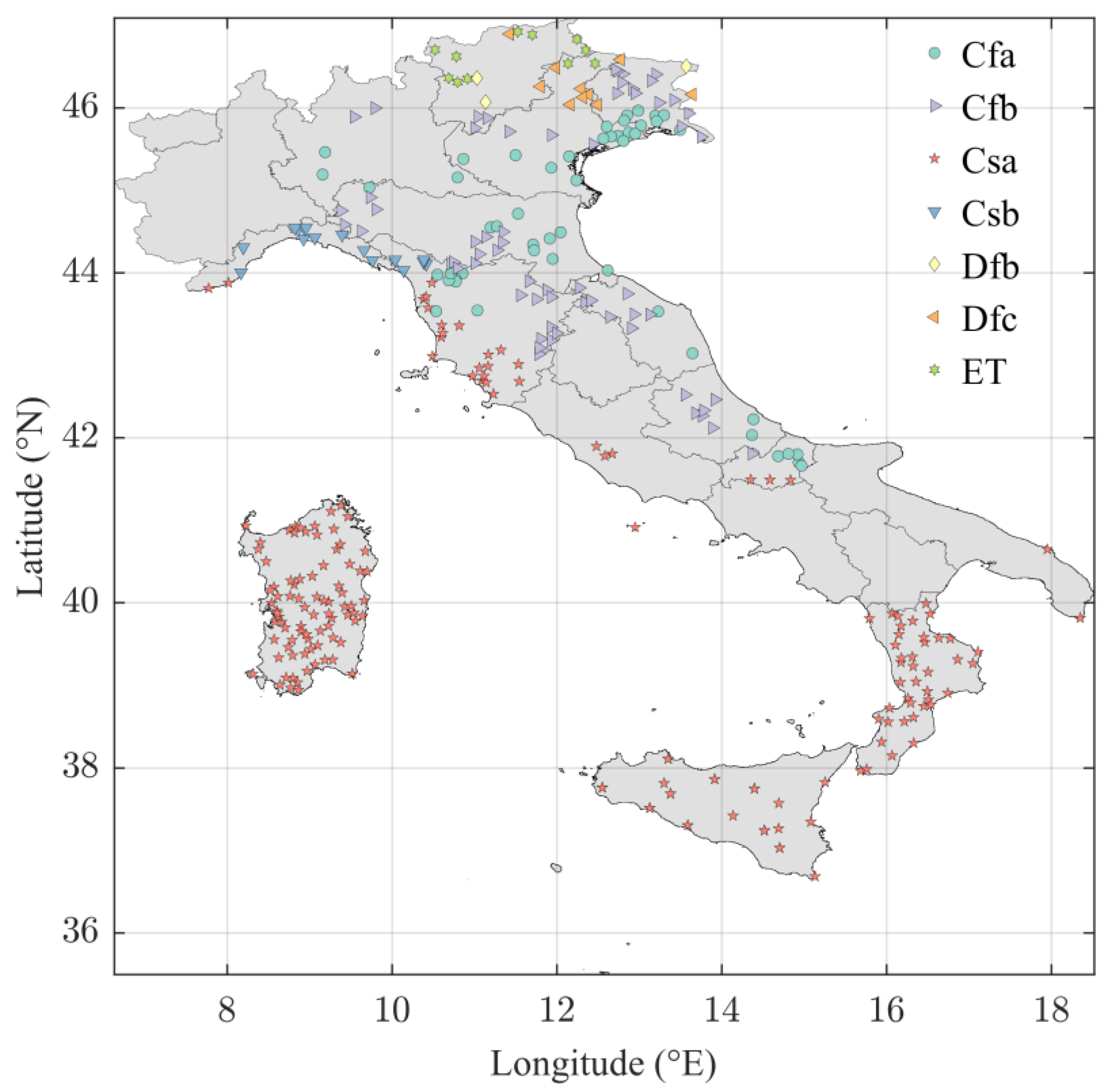
Italy has held a crucial role in the development of meteorological observations [40]. The Italian National Institute for Environmental Protection and Research (ISPRA) provides a unified and open-access system, called National System for the Collection, Elaboration and Diffusion of Climatological Data (SCIA; [34]), to optimize the use of Italian’s climate data. SCIA provides, among the many hydrometeorological variables, daily rainfall data recorded by 8489 rain gauges in the period 1860–2020. Since data are collected from different sources, ISPRA implemented a quality control procedure (i.e., according with the NOAA standards [41,42]) to obtain a homogeneous and accurate dataset [43]. Nevertheless, many of the recorded time series are too short, have many missing data or have not information about coordinates and altitude. For the SPI calculation, the World Meteorological Organization [35] suggests the use of rainfall time series with at least 40 years of continuous observations, even if an optimal length of 50–60 years is considered in Guttman [18]. For these reasons, from the 8489 rain gauge stations deployed across the country, we select 332 stations that recorded continuously in the period 1951–2000 (Figure 1). This choice was motivated in order to satisfy together the needs to have as many stations and recent years as possible.
The selected stations cover almost all the Italian regions and all the different climates, and are depicted in Figure 1 with different symbols depending on the KG classification. Despite the selected stations represent only a small percentage of the entire rain gauge network, we deem that their spatial distribution and the observation period could provide interesting remarks in the evaluation of drought over the Italian peninsula in recent years.
3.3. Monthly Rainfall Main Statistics
Studying the drought phenomenon by recurring to SPI analysis requires the use of monthly rainfall time series accumulated for different time scales. In this work we aim at analyzing drought events on monthly, trimestral, semiannual, and annual basis (i.e., SPI1, −3, −6 and −12), as they are representative time scales of different drought phenomena. Since the SCIA system provides daily rainfall time series, we perform moving windows to estimate the accumulated rainfall events for each considered time scale. The original procedure for calculating SPI proposed by McKee et al. [14] and reported in Section 2 is then followed step-by-step. Following point 1 of the procedure, for each station, we obtain 12 samples (one per month) for each analyzed time scale (i.e., 1, 3, 6 and 12). Note that, the marginal distribution of a rainfall time series at monthly resolution is mixed, with a continuous part describing the non-zero monthly rainfall values, and a discrete part describing the zeros occurrence (i.e., probability dry.). Wu et al. [25] widely investigated the crucial role played by the probability dry in the SPI estimation. Their findings reveal that in low-precipitation seasons and dry climates, the presence of zeros is common and affect the normality of the SPI, which could fail in detecting drought events. Moreover, having many zeros results in a reduction of the sample size of non-zero values, thus increasing the bias and the inconsistency in the probability distribution parameters’ estimation [44]. To provide an overview of the samples’ characteristics, we calculate the following statistics: the 25th, 50th (or median), 75th percentiles, the standard deviation (SD), and the skewness of non-zero values, and the probability dry (i.e., ratio of zeros to total observations). These statistics are calculated for the monthly samples (for each time scale) of each station and their averages are given in Table 2. As expected, for the 1-month accumulation scale, we observe the highest percentage of probability dry, that has maximum values during the summer months (July and August). This aspect, with all evidence, is linked to the Italian climate features, that is mainly Mediterranean, with hot and dry summers. Long periods of no rain are observed also for the 3-months accumulation samples of August and September (i.e., June-July-August and July-August-September, respectively). Another important aspect to be considered is related to the skewness of the non-zero values emerged in Table 2. Indeed, precipitation is bounded above zero and its distribution (i.e., non-zero values) is positively skewed. As expected, by increasing the accumulation period we observe a decrease in the average value of the skewness. The variability observed from the shortest to the highest accumulation periods of the main statistics suggests to further investigate the effects of fitting different probability distributions to the empirical monthly precipitation samples.
4. Methodology
The first objective of this investigation is testing if the Gamma distribution, proposed by McKee et al. [14], is actually the best distribution to fit Italian’s monthly rainfall data. For this purpose, we choose three biparametric probability distributions, in addition to the Gamma (), namely the Lognormal, the Weibull and the Normal. These distributions are common in hydrological practice, and were already tested and recommended in previous SPI studies [13,23,24,45]. We fit and compare the fitting performance using a modified Mean Square Error Norm (MSEN) thanks to its proven reliability and simplicity [46,47,48]. Then, the metrics used to quantify the differences between the SPI estimation approaches are described. Subsequently, the Shapiro-Wilk test (SW; [49]) is applied to test if the calculated SPI values are normally distributed, as they should by definition. Finally, we present the critical drought intensity-duration-frequency curves as an operative tool to quantify the return period of drought events based on their intensity and duration [31].
4.1. Tested Probability Distributions
In this work we aim at assessing to what extend the Gamma distribution is appropriate to fit the monthly rainfall records for each selected time scale, and how the distribution may affect the drought characteristics. We then test the fitting performance of the Lognormal (), the Weibull () and the Normal () distributions, with cumulative distribution functions (CDFs) provided in Table 3.
All the tested distributions are biparametric and their parameters are estimated with a numerical minimization of a modified mean square error norm (MSEN) given by Equation (5):
where is the sample size, denotes a specific month of the year, and are the empirical and the theoretical exceedance probabilities of the monthly rainfall amount . The main advantage of this method is that it allows the simultaneous estimation of the unknown parameters and the identification of the best suitable distribution, between the candidates, for each analyzed sample [19,46,47,48].
Since a monthly sample of rainfall data might contains several zero values, it is necessary to calculate the unconditional probability with the formulation proposed by Thom [50]:
where is the probability of zero precipitation, or probability dry, and is the fitted probability distribution. Following what introduced, the last step concerns the SPI calculation, as ; where is the quantile function of the standard normal distribution.
4.2. Quantifying the Differences between the SPI Estimation Approaches
Once the best fitting distribution for each sample is identified, it is possible to distinguish two different approaches for the SPI calculation: the standard approach (SA) proposed by McKee et al. [14], and the best fitting approach (BFA). The ability of both approaches in detecting wet and dry conditions can be tested by analyzing several aspects. As a first comparison we calculate the Pearson correlation coefficient and the Mean Bias Error , where are the SPI scores, and the number of months. Particularly, measures the linear correlation between two variables, while MBE is the degree to which the mean of a variable differs from another. Particularly, based on the formulation used, positive values of MBE indicate that the BFA estimates larger absolute SPI values than the SA, the opposite is valid for negative values.
4.3. Test of Normality: The Shapiro-Wilk Test
The Shapiro-Wilk test (SW; [49]) allows to test if the calculated SPI values are normally distributed. The SW test assumes that the resultant drought index should be normally distributed , ) and independently sampled, as each distribution is fitted based on a given month in different years. This test is widely used in literature to test the normality of the SPI [8,13,23]. According to Wu et al. [25], a distribution is considered non-normal when its variables meet the following criteria:
- Shapiro-Wilk statistic () lower than 0.96;
- p-value associated to lower than 0.10;
- absolute value of the SPI median greater than 0.05;
Where the statistic of the test is the ratio of the best estimator of the variance (based on the square of a linear combination of the order statistics) to the usual corrected sum of squares estimator of the variance. The p-value is the probability associated to the statistic.
4.4. Critical Drought Intensity-Duration-Frequency (IDF) Curves
Drought IDF curves are a technical tool useful for associating a return period (RP) to a drought event. In this work, we follow the detailed procedure proposed by Aksoy et al. [31] to build SPI-based critical drought IDF curves. These curves are based on the concept of critical drought, that is the most severe drought event for each duration occurred in each year. Based on the Aksoy et al. [31] work, the implementation of the critical drought IDF curves can be summarize with the following steps:
- SPI estimation for each time scale to distinguish dry and wet periods and to identify drought events;
- determination of the critical drought severity for all the identified drought events;
- frequency analysis of critical drought severity with the identification of the best fit probability distribution function to describe each sample. Particularly, here we used the first two Extreme Value Distribution functions, that are, the Gumbel and the Fréchet, whose parameters are determined with the MSEN method, which also aim at defining the best fitting one;
- calculation of severity and/or intensity of critical drought of a given duration for a fixed return period from the best fit probability distribution (previously identified at point iii);
- drought intensity can be expressed, for each return period, by using a linear regression line: , where is the duration (which varies between 1 month and the maximum observed), while and are coefficients determinable with curve fitting.
5. Results
5.1. Fitting Performance
As first purpose we aim at testing the performance of four probability distributions to fit the monthly data and the implication in terms of drought characteristics. To fit and compare the four tested distributions, we use the MSEN method by the numerical minimization of Equation (5). The resulting MSEN value allows the direct identification of the best fitting distribution, that is the one that realized the lowest MSEN. In Table 4, we show the percentage of stations, for each month and for all the time scales , for which the four tested distributions are the best fitting. In Figure S1 of the Supplementary Material we report an example of the fitting performance by plotting for each month all the four tested CDFs.
In general, from Table 4 emerge that the Lognormal distribution performs best for almost all the time scales and the months, followed by the Weibull and the Gamma. Particularly, for the lowest time scale (i.e., 1-month), the Weibull results the most selected distribution after the Lognormal. By increasing the time scale (up to 12-months), the Gamma and the Weibull share the remaining percentage of stations that are not best fitted by the Lognormal. As expected, the Normal distribution is the one providing the best fitting to a very low percentage of stations. This find its rationale into the skewed behaviour of the precipitation, that, even on an annual base, is not normally distributed. The good performance of the Weibull for small time scales is attributable to its ability in modelling highly skewed distributions that are typical of small accumulation periods.
5.2. Comparison of the SPI Values Estimated with the Two Different Approaches
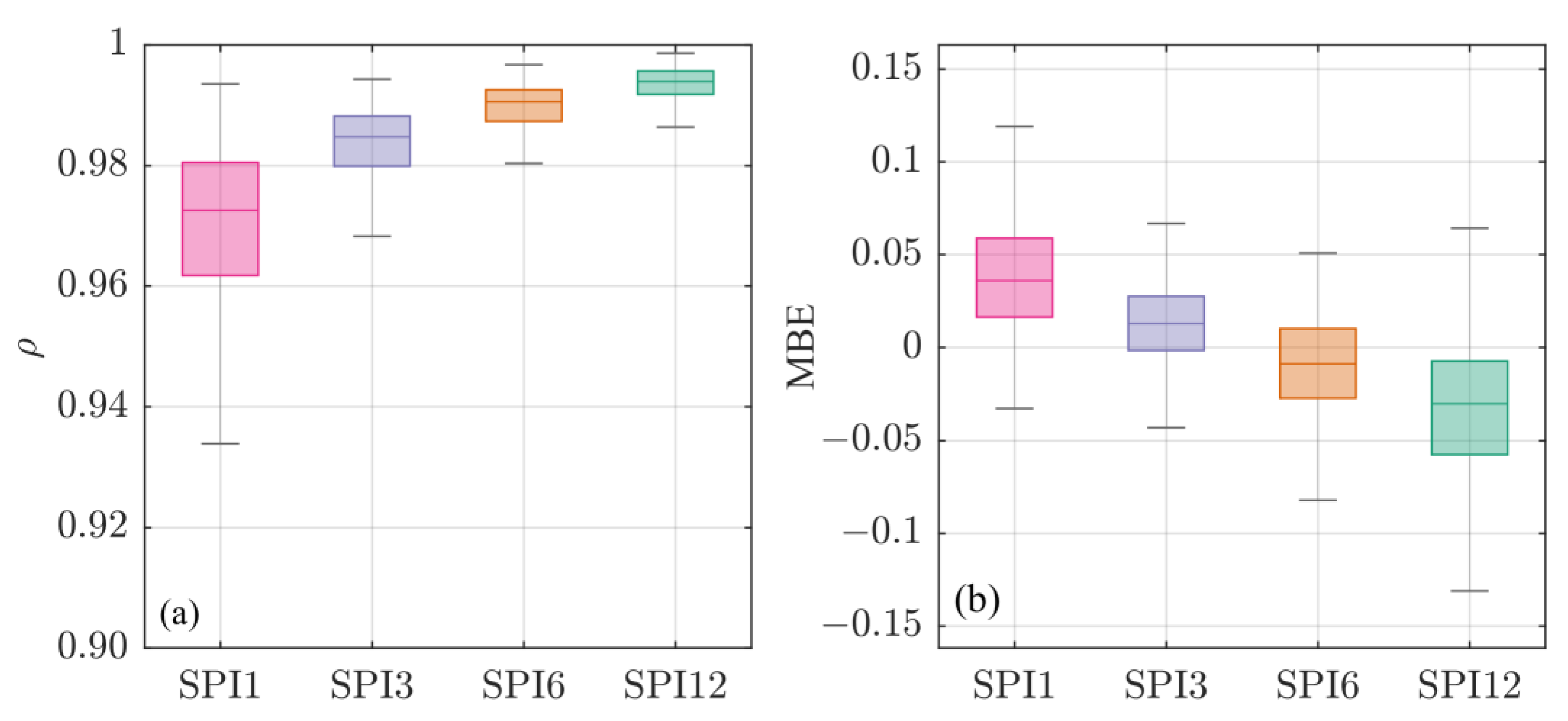
In this section we estimate the SPI using the standard approach (SA) proposed by McKee et al. [14] and a procedure based on the best probability distribution (BFA). In Figure 2 we depict a box plot for and MBE evaluated for each time scale. From Figure 2a we observe higher values of by increasing the SPI time scale, which means that the two SPI12 are almost perfectly correlated (with a median value greater than 0.99). The lowest time scale presents a median value of which is also high, but with a bigger variability respect to the higher scales. In Figure 2b, we depict the results of the MBE. In this case, we observe that the BFA tends to estimate more severe SPI values for time scales up to 3-months; while the opposite occurs for the two higher accumulation periods. For the sake of clarity, in this first analysis, we are considering the entire Z score and then both the wet and dry conditions.
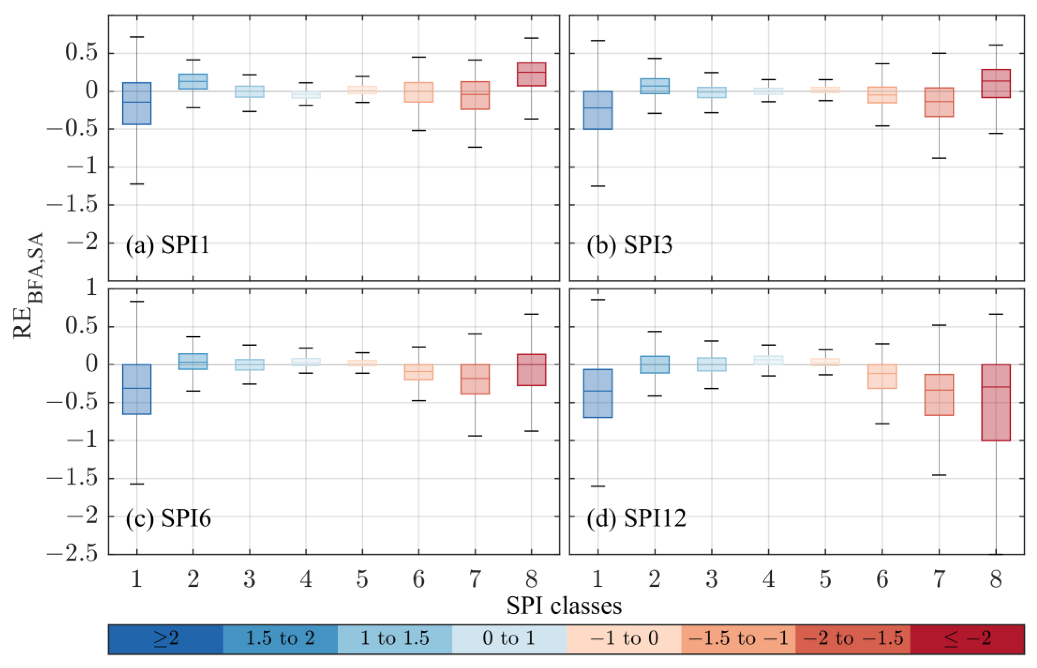
To further investigate the difference between the two approaches, we assign to each SPI value the corresponding class based on the classification provided in Table 1. In Figure 3, we show the differences obtained in the frequency distribution of wet and dry categories, respectively depicted in blue and red shades. Particularly, here we estimate the relative error , where is the class of SPI (based on Table 1), and is the number of events detected by the two approaches for each class. By construction, can vary from to 1, and it is positive when the BFA detects more events than the SA and vice versa; while the perfect match between the two approaches occurs for . For all the time scales, we observe that there are no differences in the number of selected events for the central classes (i.e., mildly wet (4) and dry (5) conditions, respectively). All the differences emerge for higher SPI magnitudes, particularly on severe and extreme classes. By focusing on the extreme dry category (i.e., 8) we can confirm what observed from the MBE results. Indeed, for SPIs up to 3-months (Figure 3a,b), the median value of the extreme category is slightly positive, confirming the general identification of more severe events detected by the BFA than the SA. The opposite instead occurs for the greatest SPI scale, where the SA detects more extreme events than the BFA (negative median value in Figure 3d). For dry events with moderate to severe magnitudes (i.e., 6 and 7 classes), the median values of are almost zero for SPI1 and decrease by increasing the time scale. This means that, in general, the SPI evaluated with the SA detects more severe drought events than the BFA for almost all the time scales. Even if this could seem in contrast with MBE results, however, in the MBE evaluation we were comparing the entire SPI score, without the possibility to consider drought and wet events separately. By focusing on the wet extreme conditions (class 1), we can see that the median value is always negative, reflecting that the SA tends to identify more extreme wet events than the BFA for all the time scales. This tendency in the two lower scales (i.e., up to SPI3), is balanced by the positive medians of the other classes, resulting in a positive . On the contrary, for SPI6 and SPI12, this tendency is amplified, since for almost all the classes the SA detects more events than the BFA, confirming the negative median value of MBE (Figure 2b).
The differences emerged from Figure 2 and Figure 3 can be attributable to both the choices of the best fitting distribution and to the parameters’ estimation method. The MLE method, indeed, finds the most likelihood couple of parameters which can represents the observed samples; while the MSEN method determines the couple of parameters which provide the best fitting of the observed data.
5.3. Drought Characteristics Comparison
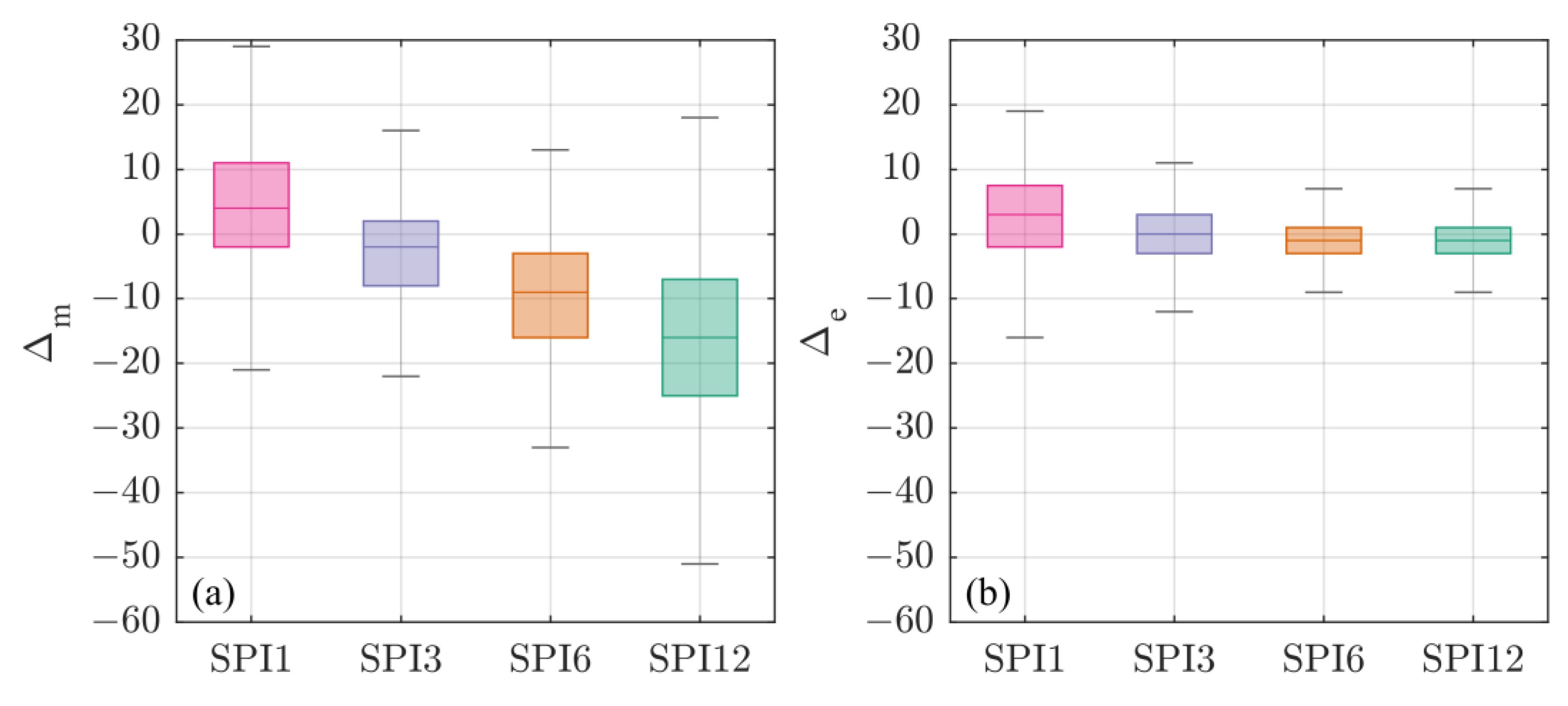
Based on the results in terms of , MBE, and on the entire SPI scores, here we compute a further investigation to quantify the differences on the drought characteristics. Particularly, we estimate: (i) the number of drought events, that is, the total number of time when SPI falls down a chosen drought threshold of ; (ii) the number of drought months; (iii) the duration (D); (iv) the severity (S); and (v) the interarrival time (T). As a first comparison, in Figure 4 we depict the difference in terms of the total number of drought months () and events () detected by the two approaches for all the time scales. In both cases, positive values means that the BFA detects more drought months or events than the SA. Similarly to the previous analysis, for SPI up to 3-months the BFA estimates more drought months and events than the SA, and the opposite is valid for longer scales (i.e., 6 and 12-months). It is interesting to highlight the differences in terms of variability between the two measures. Indeed, the difference in drought months presents a higher variability than the difference in drought events. This is due to the presence of single drought months detected from one approach but not from the other. On the contrary, when we analyze drought events, they could have a different duration in months, but the general behaviour between the two approaches is similar, according to the good performance emerged from the Pearson correlation coefficient (Figure 2a). For more details on the spatial variability of and please refer to Figures S2 and S3 of the Supplementary Material, respectively.
In addition to the number of drought months and events, in Table 5 we report the variability of the severity (S), the duration (D), and the interarrival time between two consequent drought events (T) for each approach. For the sake of clarity, the main statistics of all the characteristics are estimated considering all the values for all the stations. Coherently with the previous findings, we observe that for SPI1 and SPI3, in general, the main statistics of the BFA are larger than the SA, while the opposite is valid for larger scales.
5.4. Normality Test
For its definition, the SPI should be normally distributed with zero expected value and variance one. However, this is not always the case for SPI at short time scales, because of the skewed precipitation distribution [15]. Indeed, in dry seasons and dry climates, the presence of many zeros in the monthly sample will result in a non-normal distributed SPI [51]. Here we test the normality of the SPI estimated with both the approaches, for every month of the year and for each time scale by applying the Shapiro Wilk test. In Table 6 we report the percentage of stations whose SPI resulted non-normal distributed. As expected, for the lowest time scale (i.e., k = 1) and for both the approaches, we obtain the highest percentage of stations whereby the SPI is characterized by a non-normal behaviour. As a general remark, the BFA produces a higher percentage of non-normal SPIs respect to the SA.
This characteristic is not specific of regions with dry climate (for the location of the non-normal SPI samples see the maps in Figure S4 of the Supplementary material), but it can be due to a seasonal phenomenon. To provide a few examples, in Sicily we have non-normal series even during the winter months, while in Emilia-Romagna and in Trentino Alto Adige non-normality is related also to summer months. Moreover, the non-normal behaviour appears in both the investigated approaches thus, the use of the best fitting distribution does not attenuate the results but makes them worse. Interestingly, SPI appears non-normal distributed also for time scales > 3 even if there are no zeros in the monthly precipitation series analyzed. Indeed, the presence of zeros is typical of the summer months (i.e., June, July, and August), and it is drastically reduced when the precipitation series are aggregated. For the 332 stations analyzed in this work, zeros appear only at 1-month and 3-months series (as shown in Table 2).
The high probability of no-rain cases represents the main cause of the non-normal distribution of SPI, together with a limited sample size. Indeed, for construction, when data samples are characterized by many zeros, the resulted SPI is always greater than a specific value (i.e., bounded below). For this reason, the presence of many zeros in specific months of the year results in associating a high probability, and then a high SPI value, to a very small amount of precipitation. For this reason, as also suggested by Wu et al. [22], the use of the SPI in arid areas should be limited to the evaluation of drought duration rather than its severity to avoid significant errors.
5.5. Critical Drought IDF Curves
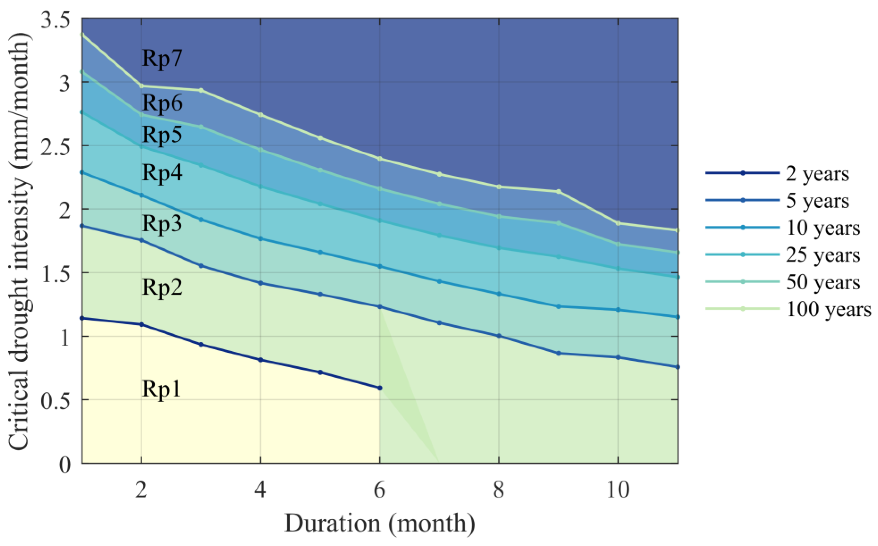
As a final comparison between the two approaches, we build the critical drought IDF curves that allows to quantify and review the differences in the drought characteristics emerged from the previous analysis. Particularly, with these curves, we intent to give an objective interpretation of the observed drought events thanks to the use of the return period (RP). Based on the procedure proposed by Aksoy et al. [31], for both the SA and the BFA, for all the stations and all the time scales, we determine the critical drought IDF curves for six fixed return periods (i.e., 2, 5, 10, 25, 50 and 100 years). Then, for each station and each time scale, we define seven return period classes (Rp) bounded by the critical drought IDF curves (Figure 5). Thanks to this classification, we calculate the percentage of events detected by the two approaches lying in a specific return period interval. Basically, given a drought event with a specific intensity and duration, it is possible to directly associate the class in which it falls, by simply placing a point in the graph. It is important to clarify that, the critical drought IDF plotted in Figure 5 are those obtained by linking the critical drought intensities obtained for each duration, thus without the empirical curve fitting described at point v of Section 4.4. For the sake of clarity, in this analysis we multiply by the intensities obtained by the product of severity and duration. For this reason, in Figure 5 the positive intensities are related to drought values (contrary to the typical symbology of the SPI).
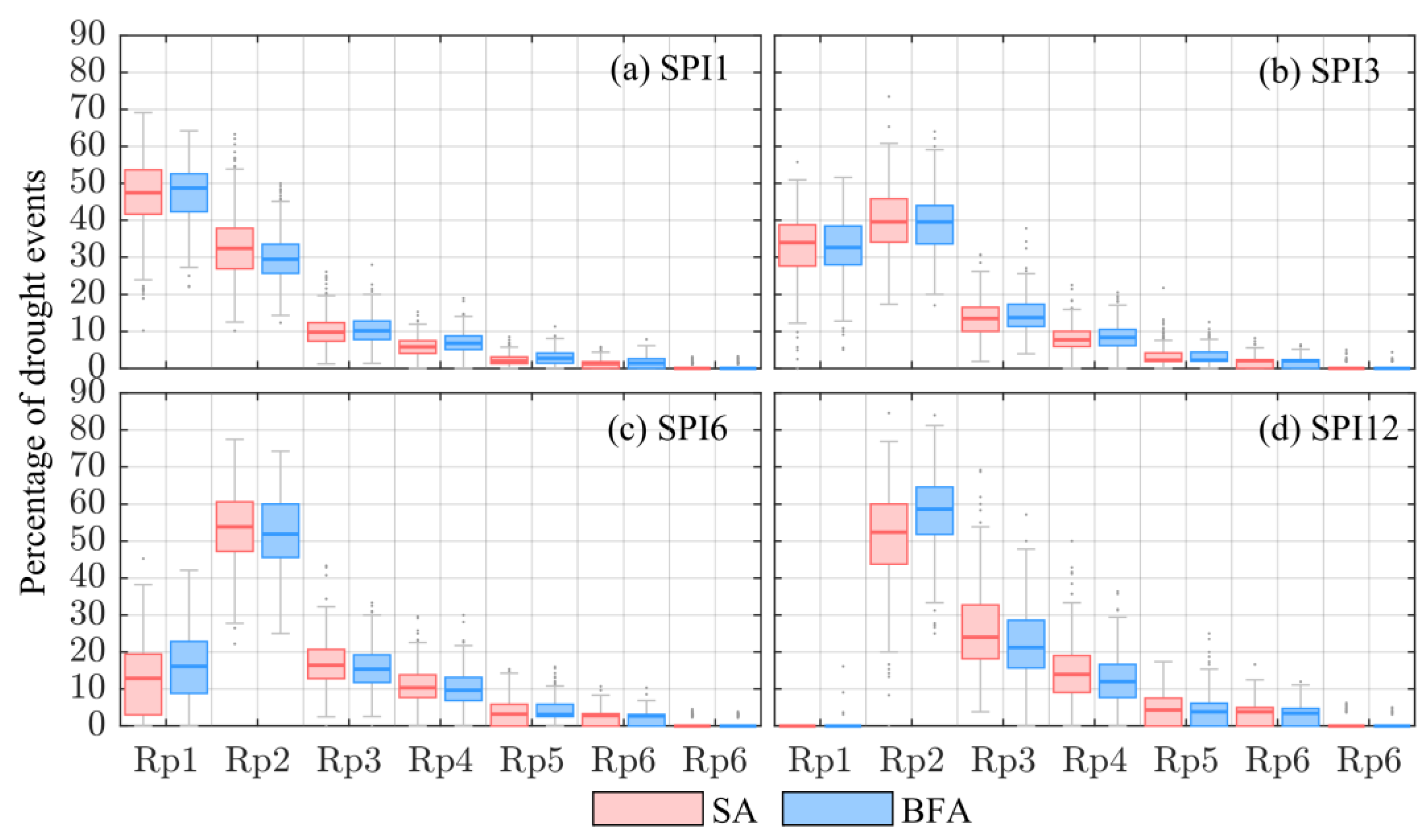
In Figure 6, we represent the percentage of drought events detected by the BFA and the SA lying in each Rp class. Despite the differences between the two approaches in detecting the characteristic of drought emerged previously, in Figure 6 we observe that the drought events belong, in general, to the same Rp class. Indeed, median values and variance are similar for almost all the Rp classes and SPI time scale. The maximum percentage difference between the two approaches is observed in Figure 6d for SPI12. In this case, the BFA identify more events between 2 years and 5 years return periods (i.e., Rp2) respect to the SA (the two median values differ by 6.2%). The opposite can be seen for the other classes (with differences of the median values less than 2%).
The last analysis is the comparison between the two coefficients of the linear regression line describing the link between intensity, duration and return period (point v of the procedure described in Section 4.4). Particularly, we compare all and values obtained from all the 332 stations for each SPI time scale. We present the differences in terms of (Table 7), which is the angular deviation of the representative line of the cloud of points from the maximum agreement line (for more details on the procedure please see Figure S5 of the Supplementary material). Positive values indicate that, generally, the critical drought IDF curves obtained from the BFA present greater and values than the SA, and vice versa. Higher values lead to steeper IDF curves, while, for a given duration, high values of indicate higher intensities.
As a result, in Table 7 we observe that almost all the values, for both and , are positive, indicating that in general the BFA tends to produce steeper and higher critical drought IDF then the SA. Coherently with the other comparisons, to lower SPI time scales are associated the widest differences. As expected, by increasing the return period, the differences between the two approaches increase.
6. Discussion and Conclusions
García-León et al. [45] estimated that the drought-induced economic losses in Italy ranged between 0.55 and 1.75 billion euros in the period 2001–2016. In addition, the IPCC declared that drought events are expected to increase in frequency and intensity due to global warming [52]. Studying and understanding droughts is than necessary to tackle its socio-economic and environmental impacts. The Standardized Precipitation Index (SPI) is the recommended index to characterize droughts worldwide [35]. Although this index has several strengths, such as precipitation as the only input and the possibility to be computed for different time scales and for all climates, it marks some drawbacks as well. In facts, it can only quantify the precipitation deficit, without considering other important physical aspects (i.e., evapotranspiration), moreover its reliable assessment is influenced by the available period of observations (i.e., time series record length) [53]. Nevertheless, the use of the SPI is widespread, since it allows to provide early warning of drought and helps assess drought severity [35].
In this study we questioned the standard approach (SA) of the SPI estimation proposed by McKee et al. [14], that is, fitting a Gamma distribution to monthly precipitation data for each aggregated monthly time scale. We tested a different method to estimate the SPI, by choosing the best fitting probability distribution (BFA) to describe the empirical monthly samples before the equiprobability transformation. The study was conducted using precipitation series recorded by an unprecedent dataset consisting of daily rainfall records from 332 rain gauges in the period 1951–2000 (i.e., 50 continuous years of observation) in Italy. The results of our analysis can be summarized as follows.
- The Lognormal distribution resulted to be the best fit model to describe almost all the monthly precipitation samples, followed by the Weibull (for 1-month scale) and the Gamma. The Normal distribution, as expected, resulted as the best fitted for a very low percentage of stations, confirming its poor ability in modelling samples with a positive skewness;
- the Pearson Correlation Coefficient ( evaluated on the entire SPI signal, showed an almost perfect agreement between the SPI signals estimated by the two tested approaches for 12-months time scale. Median values decrease by reducing the SPI’s time scale till 0.97 for SPI1 (Figure 2a);
- the Mean Bias Error (MBE) indicated an opposite behaviour for lower and higher SPI’s time scale. Indeed, for time scales up to 3-months, the BFA presented more severe SPI values than the SA, while the opposite was observed for 6- and 12-months scales;
- by highlighting the differences between the two approaches in detecting both wet and dry periods, the Relative Error (RE) followed the behaviour of the MBE: the BFA tends to detect more extreme conditions than the SA for lower scales (i.e., SPI1 and SPI3), and vice versa for SPI6 and SPI12;
- the same patterns emerged from the analysis of the entire SPI signal are reflected on the analysis of drought events (i.e., SPI ≤ −1). Generally, the SA under-estimates all the drought characteristics (i.e., number of events and number of drought months (Figure 4), duration, severity and interarrival time (Table 5)) for small time scales (up to 3-months), while for longer time scale over-estimates the same characteristics. Clearly, we consider as a benchmark the BFA, since it is built to provide the best model to describe the empirical samples;
- the use of the BFA did not solve the SPI non-normality issue, indeed the percentage of non-normal SPIs is higher than the SA for all the months and all the time scales;
- despite the differences between the two approaches emerged in drought characteristics, the analyzed drought events lie in the same return period classes (Figure 6) for all the time scales.
As a general remark, we believe that using a unique model to fit monthly rainfall data recorded in different areas with different climates should be performed with caution. Based on the results obtained in this work, from a theoretical point of view, testing several probability distributions to fit the monthly empirical data should become the standard practice in the evaluation of the SPI. However, the differences in terms of drought characteristics are negligible when the events analysis is performed with critical drought IDF curves. Indeed, the events detected by the two approaches belong to the same return period classes, indicating no evident differences in terms of drought risk assessment and management. We believe that this study could provide interesting insight into the drought characterization in Italy. Moreover, the proposed methodology can support the mitigation and monitoring of drought risk even in more recent years, and help facing the challenges of a high Anthropogenic era.
Supplementary Materials
The following supporting information can be downloaded at: https://www.mdpi.com/article/10.3390/w14223668/s1, Table S1: information on the 332 stations selected from the SCIA system; Figure S1: fitting performance of the four tested probability distributions to 3-months precipitation samples for the Roma/Ciampino station; Figure S2: maps showing the difference in terms of number of drought months detected by the two approaches for all the time scales; Figure S3: maps showing the difference in terms of number of events detected by the two approaches for all the time scales; Figure S4: maps showing the location of the non-normal distributed SPI signals for both the approaches; Figure S5: explanation of the comparison method based on angle.
Author Contributions
Conceptualization, B.M., C.M. and F.R.; methodology, B.M., C.M., E.R. and F.N.; software, B.M.; formal analysis, B.M., C.M. and E.R.; data curation, B.M.; writing—original draft preparation, B.M., C.M. and E.R.; writing—review and editing, B.M., C.M. and E.R.; visualization, B.M.; supervision, F.R. and F.N. All authors have read and agreed to the published version of the manuscript.
Funding
The research is partially supported by Autorità di Bacino Distrettuale Appennino Centrale.
Data Availability Statement
The daily rainfall data used in this work are freely available at http://www.scia.isprambiente.it (accessed 10 September 2022). A list of the stations used in this work is provided in Table S1.
Acknowledgments
The authors would like to express their sincere gratitude to Eleonora Boscariol for her precious contribution in the implementation of the critical drought IDF curves methodology. The authors are also thankful for the comments and suggestions provided by three anonymous reviewers that contributed to consistently improve the paper.
Conflicts of Interest
The authors declare no conflict of interest.
References
- Baronetti, A.; González-Hidalgo, J.C.; Vicente-Serrano, S.M.; Acquaotta, F.; Fratianni, S. A weekly spatio-temporal distribution of drought events over the Po Plain (North Italy) in the last five decades. Int. J. Climatol. 2020, 40, 4463–4476. [Google Scholar] [CrossRef]
- Cancelliere, A.; Salas, J.D. Drought length properties for periodic-stochastic hydrologic data. Water Resour. Res. 2004, 40, 1–13. [Google Scholar] [CrossRef]
- Kreibich, H.; Van Loon, A.F.; Schröter, K.; Ward, P.J.; Mazzoleni, M.; Sairam, N.; Abeshu, G.W.; Agafonova, S.; AghaKouchak, A.; Aksoy, H.; et al. The challenge of unprecedented floods and droughts in risk management. Nature 2022, 608, 80–86. [Google Scholar] [CrossRef] [PubMed]
- Burgan, H.I.; Aksoy, H. Daily flow duration curve model for ungauged intermittent subbasins of gauged rivers. J. Hydrol. 2022, 604, 127249. [Google Scholar] [CrossRef]
- Lloyd-Hughes, B.; Saunders, M.A. A drought climatology for Europe. Int. J. Climatol. 2002, 22, 1571–1592. [Google Scholar] [CrossRef]
- Garcia, M.; Ridolfi, E.; Di Baldassarre, G. The interplay between reservoir storage and operating rules under evolving conditions. J. Hydrol. 2020, 590, 125270. [Google Scholar] [CrossRef]
- American Meteorological Society (AMS). Statement on meteorological drought. Bull. Am. Meteorol. Soc. 2004, 85, 771–773. [Google Scholar]
- Kumar, M.N.; Murthy, C.S.; Sesha Sai, M.V.R.; Roy, P.S. On the use of Standardized Precipitation Index (SPI) for drought intensity assessment. Meteorol. Appl. 2009, 16, 381–389. [Google Scholar] [CrossRef] [Green Version]
- Van Loon, A.F. Hydrological drought explained. WIREs Water 2015, 2, 359–392. [Google Scholar] [CrossRef]
- Liu, X.; Zhu, X.; Pan, Y.; Li, S.; Liu, Y.; Ma, Y. Agricultural drought monitoring: Progress, challenges, and prospects. J. Geogr. Sci. 2016, 26, 750–767. [Google Scholar] [CrossRef] [Green Version]
- Zhao, M.; Huang, S.; Huang, Q.; Wang, H.; Leng, G.; Xie, Y. Assessing socio-economic drought evolution characteristics and their possible meteorological driving force Assessing socio-economic drought evolution characteristics and their possible meteorological driving force. Geomat. Nat. Hazards Risk 2019, 10, 1084–1101. [Google Scholar] [CrossRef]
- Mishra, A.K.; Singh, V.P. A review of drought concepts. J. Hydrol. 2010, 391, 202–216. [Google Scholar] [CrossRef]
- Stagge, J.H.; Tallaksen, L.M.; Gudmundsson, L.; Van Loon, A.F.; Stahl, K. Candidate Distributions for Climatological Drought Indices (SPI and SPEI). Int. J. Climatol. 2015, 35, 4027–4040. [Google Scholar] [CrossRef]
- McKee, T.B.; Doesken, N.J.; Kleist, J. The Relationship of Drought Frequency and Duration to Time Scales. In Proceedings of the 8th Conference on Applied Climatology, Anaheim, CA, USA, 17–22 January 1993; Volume 17, pp. 179–183. [Google Scholar]
- Edwards, D.C.; McKee, T.B. Characteristics of 20th century drought in the United States at multiple time scales. In Atmospheric Science Paper 634; Department of Atmospheric Science, Colorado State University: Fort Collins, CO, USA, 1997. [Google Scholar]
- Papalexiou, S.M.; Rajulapati, C.R.; Andreadis, K.M.; Foufoula-Georgiou, E.; Clark, M.P.; Trenberth, K.E. Probabilistic Evaluation of Drought in CMIP6 Simulations. Earths Future 2021, 9, e2021EF002150. [Google Scholar] [CrossRef] [PubMed]
- Wu, H.; Hayes, M.J.; Wilhite, D.A.; Svoboda, M.D. The effect of the length of record on the standardized precipitation index calculation. Int. J. Climatol. 2005, 25, 505–520. [Google Scholar] [CrossRef] [Green Version]
- Guttman, N.B. Accepting the standardized precipitation index: A calculation algorithm. J. Am. Water Resour. Assoc. 1999, 35, 311–322. [Google Scholar] [CrossRef]
- Mineo, C.; Moccia, B.; Lombardo, F.; Russo, F.; Napolitano, F. Preliminary Analysis About the Effects on the SPI Values Computed from Different Best-Fit Probability Models in Two Italian Regions. In New Trends in Urban Drainage Modelling, Green Energy and Technology; Springer: Cham, Switzerland, 2018; pp. 958–962. [Google Scholar] [CrossRef]
- Sol’áková, T.; De Michele, C.; Vezzoli, R. Comparison between Parametric and Nonparametric Approaches for the Calculation of Two Drought Indices: SPI and SSI. J. Hydrol. Eng. 2014, 19, 04014010. [Google Scholar] [CrossRef]
- Angelidis, P.; Maris, F.; Kotsovinos, N.; Hrissanthou, V. Computation of Drought Index SPI with Alternative Distribution Functions. Water Resour. Manag. 2012, 26, 2453–2473. [Google Scholar] [CrossRef]
- Guenang, G.M.; Mkankam Kamga, F. Computation of the standardized precipitation index (SPI) and its use to assess drought occurrences in Cameroon over recent decades. J. Appl. Meteorol. Climatol. 2014, 53, 2310–2324. [Google Scholar] [CrossRef]
- Vergni, L.; Di Lena, B.; Todisco, F.; Mannocchi, F. Uncertainty in drought monitoring by the Standardized Precipitation Index: The case study of the Abruzzo region (central Italy). Theor. Appl. Climatol. 2017, 128, 13–26. [Google Scholar] [CrossRef]
- Mahmoudi, P.; Ghaemi, A.; Rigi, A.; Amir Jahanshahi, S.M. Recommendations for modifying the Standardized Precipitation Index (SPI) for Drought Monitoring in Arid and Semi-arid Regions. Water Resour. Manag. 2021, 35, 3253–3275. [Google Scholar] [CrossRef]
- Wu, H.; Svoboda, M.D.; Hayes, M.J.; Wilhite, D.A.; Wen, F. Appropriate application of the standardized precipitation index in arid locations and dry seasons. Int. J. Climatol. A J. R. Meteorol. Soc. 2007, 27, 65–79. [Google Scholar] [CrossRef]
- Rahmat, S.N.; Jayasuriya, N.; Bhuiyan, M. Development of drought severity-duration-frequency curves in Victoria, Australia. Aust. J. Water Resour. 2015, 19, 31–42. [Google Scholar] [CrossRef] [Green Version]
- Bonaccorso, B.; Cancelliere, A.; Rossi, G. An analytical formulation of return period of drought severity. Stoch. Environ. Res. Risk Assess. 2003, 17, 157–174. [Google Scholar] [CrossRef]
- Dalezios, N.R.; Loukas, A.; Vasiliades, L.; Liakopoulos, E. Severity-duration-frequency analysis of droughts and wet periods in Greece. Hydrol. Sci. J. 2000, 45, 751–769. [Google Scholar] [CrossRef]
- Bertini, C.; Buonora, L.; Ridolfi, E.; Russo, F.; Napolitano, F. On the Use of Satellite Rainfall Data to Design a Dam in an Ungauged Site. Water 2020, 12, 3028. [Google Scholar] [CrossRef]
- Aksoy, H.; Onoz, B.; Cetin, M.; Yuce, M.I. SPI-based Drought Severity-Duration-Frequency Analysis. In Proceedings of the 13th International Congress on Advances in Civil Engineering, Izmir, Turkey, 12–14 September 2018. [Google Scholar]
- Aksoy, H.; Cetin, M.; Eris, E.; Burgan, H.I.; Cavus, Y.; Yildirim, I.; Sivapalan, M. Critical drought intensity-duration-frequency curves based on total probability theorem-coupled frequency analysis. Hydrol. Sci. J. 2021, 66, 1337–1358. [Google Scholar] [CrossRef]
- Cavus, Y.; Aksoy, H. Critical drought severity/intensity-duration-frequency curves based on precipitation deficit. J. Hydrol. 2020, 584, 124312. [Google Scholar] [CrossRef]
- Song, S.; Singh, V.P.; Song, X.; Kang, Y. A probability distribution for hydrological drought duration. J. Hydrol. 2021, 599, 126479. [Google Scholar] [CrossRef]
- Desiato, F.; Lena, F.; Toreti, A. SCIA: A system for a better knowledge of the Italian climate. Boll. Geofis. Teor. Appl. 2007, 48, 351–358. [Google Scholar]
- Svoboda, M.; Hayes, M.; Wood, D. Standardized Precipitation Index: User Guide; World Meteorological Organization: Geneva, Switzerland, 2012. [Google Scholar]
- Fratianni, S.; Acquaotta, F. The Climate of Italy. In World Geomorphological Landscapes; Springer: Cham, Switzerland, 2017; pp. 29–38. ISBN 9783319261942. [Google Scholar]
- Kottek, M.; Grieser, J.; Beck, C.; Rudolf, B.; Rubel, F. World map of the Köppen-Geiger climate classification updated. Meteorol. Z. 2006, 15, 259–263. [Google Scholar] [CrossRef]
- Peel, M.C.; Finlaysonm, B.L.; McMahon, T.A. Updated world map of the Köppen-Geiger climate classification. Hydrol. Earth Syst. Sci. 2007, 11, 1633–1644. [Google Scholar] [CrossRef] [Green Version]
- Moccia, B.; Papalexiou, S.M.; Russo, F.; Napolitano, F. Spatial variability of precipitation extremes over Italy using a fine-resolution gridded product. J. Hydrol. Reg. Stud. 2021, 37, 100906. [Google Scholar] [CrossRef]
- Brunetti, M.; Maugeri, M.; Monti, F.; Nanni, T. Temperature and precipitation variability in Italy in the last two centuries from homogenised instrumental time series. Int. J. Climatol. 2006, 26, 345–381. [Google Scholar] [CrossRef]
- Durre, I.; Menne, M.J.; Gleason, B.E.; Houston, T.G.; Vose, R.S. Comprehensive automated quality assurance of daily surface observations. J. Appl. Meteorol. Climatol. 2010, 49, 1615–1633. [Google Scholar] [CrossRef] [Green Version]
- Arguez, A.; Durre, I.; Applequist, S.; Vose, R.S.; Squires, M.F.; Yin, X.; Heim, R.R.; Owen, T.W. Noaa’s 1981-2010 U.S. climate normals. Bull. Am. Meteorol. Soc. 2012, 93, 1687–1697. [Google Scholar] [CrossRef]
- Fioravanti, G.; Fraschetti, P.; Perconti, W.; Piervitali, E.; Desiato, F. Controlli di qualità delle serie di temperatura e precipitazione. In Rapporto ISPRA/Stato dell’Ambiente 66/2016; ISPRA: Roma, Italy, 2016. [Google Scholar]
- Nerantzaki, S.; Papalexiou, S.M. Assessing Extremes in Hydroclimatology: A Review on Probabilistic Methods. J. Hydrol. 2022, 605, 127302. [Google Scholar] [CrossRef]
- García-León, D.; Standardi, G.; Staccione, A. An integrated approach for the estimation of agricultural drought costs. Land Use Policy 2021, 100, 104923. [Google Scholar] [CrossRef]
- Papalexiou, S.M.; Koutsoyiannis, D.; Makropoulos, C. How extreme is extreme? An assessment of daily rainfall distribution tails. Hydrol. Earth Syst. Sci. 2013, 17, 851–862. [Google Scholar] [CrossRef] [Green Version]
- Moccia, B.; Mineo, C.; Ridolfi, E.; Russo, F.; Napolitano, F. Probability distributions of daily rainfall extremes in Lazio and Sicily, Italy, and design rainfall inferences. J. Hydrol. Reg. Stud. 2021, 33, 100771. [Google Scholar] [CrossRef]
- Gupta, N.; Chavan, S.R. Assessment of temporal change in the tails of probability distribution of daily precipitation over India due to climatic shift in the 1970s. J. Water Clim. Chang. 2021, 12, 2753–2773. [Google Scholar] [CrossRef]
- Shapiro, S.S.; Wilk, M.B. An Analysis of Variance Test for Normality (Complete Series). Biometrika 1965, 52, 591–611. [Google Scholar] [CrossRef]
- Thom, H.C.S. A Note on the Gamma Distribution. Mon. Weather. Rev. 1958, 86, 117–122. [Google Scholar] [CrossRef]
- Barger, G.L.; Shaw, R.H.; Dale, R.F. Chances of Receiving Selected Amounts of Precipitation in the North Central Region of the United States; Agricultural and Home Economics Experimental Station: Ames, IA, USA; Iowa State University: Ames, IA, USA, 1959. [Google Scholar]
- Allan, R.P.; Hawkins, E.; Bellouin, N.; Collins, B. IPCC, 2021: Summary for Policymakers. In Climate Change 2021: The Physical Science Basis. Contribution of Working Group II to the Sixth Assessment Report of the Intergovernmental Panel on Climate Change; Cambridge University Press: Cambridge, UK, 2021. [Google Scholar]
- Zuo, D.D.; Hou, W.; Zhang, Q.; Yan, P.C. Sensitivity analysis of standardized precipitation index to climate state selection in China. Adv. Clim. Chang. Res. 2022, 13, 42–50. [Google Scholar] [CrossRef]
Figure 1.
Location of the 332 stations selected from the SCIA dataset. Each station is depicted with a different marker based on the Köppen-Geiger (KG) classification [37,38]. Particularly, 53.8% of the stations belong to Csa-KG, 19.2% to Cfb-KG, 15% to Cfa-KG, 4.8% to Csb-KG, 3.3% to ET-KG, 3% to Dfc-KG, and 0.9% to Dfb-KG. All the information related to the stations are provided in Table S1 of the Supplementary Material.

Figure 2.
Box plots representing the Pearson correlation coefficient (a) and the Mean Bias Error (b) between the SPI values estimated with the SA and the BFA for each time scale.
Figure 2.
Box plots representing the Pearson correlation coefficient (a) and the Mean Bias Error (b) between the SPI values estimated with the SA and the BFA for each time scale.

Figure 3.
Box plots representing the Relative Error (RE) of the number of classes detected by the SPI estimated with the BFA and SA. The horizontal zeros grey line represents the perfect match between the two approaches. Both the wet (blue-shades) and dry (red-shades) categories are depicted. The SPI classes (from 1 to 8) are ordered from the extremely wet to the extremely drought categories, according to Table 1.

Figure 4.
Variability of the differences (a) and (b) or each time scale.

Figure 5.
SPI6 critical drought IDF curves representation for CAPESTRANO-Idro station. Each shaded color represents a different Rp class, while each line is a critical drought IDF for a fixed return period (RP).
Figure 5.
SPI6 critical drought IDF curves representation for CAPESTRANO-Idro station. Each shaded color represents a different Rp class, while each line is a critical drought IDF for a fixed return period (RP).

Figure 6.
Boxplots representing the percentage of drought events detected by the two approaches lying in each return period class (Rp) for each SPI time scale.
Figure 6.
Boxplots representing the percentage of drought events detected by the two approaches lying in each return period class (Rp) for each SPI time scale.


Table 1.
Event classification based on SPI values and their probability of occurrence [14].
Table 1.
Event classification based on SPI values and their probability of occurrence [14].
| SPI Values | SPI Classes | Probability (%) |
|---|---|---|
| Extremely wet | 2.3 | |
| 1.5 to 2.00 | Severely wet | 4.4 |
| 1.0 to 1.5 | Moderately wet | 9.2 |
| 0 to 1.0 | Mildly wet | 34.1 |
| −1.0 to 0 | Mildly drought | 34.1 |
| −1.5 to −1.0 | Moderate drought | 9.2 |
| −2.0 to −1.5 | Severe drought | 4.4 |
| Extreme drought | 2.3 |
Table 2.
Mean values of the main statistics evaluated on the 332 samples for each time scale (1, 3, 6 and 12 months) and for each month. Apart from the probability dry (Pdry), these statistics are evaluated considering the non-zero monthly rainfall.
Table 2.
Mean values of the main statistics evaluated on the 332 samples for each time scale (1, 3, 6 and 12 months) and for each month. Apart from the probability dry (Pdry), these statistics are evaluated considering the non-zero monthly rainfall.
| 1-month | 3-months | ||||||||||||
| P25 | P50 | P75 | SD | Skew | Pdry | P25 | P50 | P75 | SD | Skew | Pdry | ||
| month | 1 | 41.33 | 77.35 | 121.12 | 60.56 | 0.92 | 1.3% | 219.89 | 299.01 | 387.44 | 125.34 | 0.48 | 0% |
| 2 | 35.14 | 66.98 | 110.76 | 60.12 | 1.15 | 1.0% | 190.24 | 256.97 | 332.51 | 115.73 | 0.65 | 0% | |
| 3 | 38.51 | 71.00 | 113.26 | 54.54 | 0.86 | 1.3% | 161.94 | 229.09 | 309.63 | 116.03 | 0.77 | 0% | |
| 4 | 46.19 | 72.74 | 106.42 | 48.40 | 0.96 | 0.6% | 168.06 | 226.85 | 297.86 | 97.84 | 0.62 | 0% | |
| 5 | 35.48 | 58.67 | 89.13 | 43.12 | 1.15 | 1.4% | 164.54 | 217.10 | 277.25 | 85.09 | 0.54 | 0% | |
| 6 | 32.41 | 49.19 | 72.62 | 35.60 | 1.52 | 6.3% | 149.18 | 193.92 | 246.78 | 74.29 | 0.58 | 0% | |
| 7 | 22.04 | 35.92 | 56.22 | 30.22 | 1.52 | 19.1% | 116.45 | 152.24 | 198.02 | 63.72 | 0.89 | 0% | |
| 8 | 24.42 | 43.28 | 71.44 | 39.45 | 1.37 | 12.5% | 101.72 | 135.83 | 180.40 | 63.91 | 1.05 | 2% | |
| 9 | 32.93 | 62.99 | 106.11 | 58.97 | 1.25 | 2.5% | 106.64 | 153.13 | 209.85 | 82.32 | 0.96 | 1% | |
| 10 | 50.38 | 96.28 | 159.98 | 87.21 | 1.19 | 0.9% | 153.35 | 222.95 | 305.76 | 117.73 | 0.87 | 0% | |
| 11 | 64.44 | 108.52 | 164.74 | 80.37 | 1.04 | 0.5% | 212.44 | 295.89 | 389.32 | 134.99 | 0.68 | 0% | |
| 12 | 57.33 | 92.25 | 141.43 | 68.85 | 1.05 | 0.4% | 235.40 | 319.01 | 426.46 | 144.01 | 0.70 | 0% | |
| 6-months | 12-months | ||||||||||||
| P25 | P50 | P75 | SD | Skew | Pdry | P25 | P50 | P75 | SD | Skew | Pdry | ||
| month | 1 | 427.29 | 528.10 | 651.62 | 175.05 | 0.57 | 0% | 791.59 | 930.03 | 1090.20 | 217.87 | 0.48 | 0% |
| 2 | 455.31 | 560.20 | 676.80 | 173.94 | 0.57 | 0% | 796.53 | 929.64 | 1080.20 | 210.84 | 0.43 | 0% | |
| 3 | 457.76 | 564.55 | 679.86 | 174.98 | 0.46 | 0% | 801.08 | 927.79 | 1075.85 | 207.39 | 0.43 | 0% | |
| 4 | 431.31 | 533.26 | 643.87 | 160.70 | 0.51 | 0% | 801.33 | 926.70 | 1073.89 | 206.62 | 0.46 | 0% | |
| 5 | 387.32 | 478.80 | 581.76 | 150.44 | 0.52 | 0% | 799.72 | 928.24 | 1073.12 | 208.99 | 0.48 | 0% | |
| 6 | 345.38 | 431.96 | 531.22 | 142.70 | 0.50 | 0% | 799.64 | 930.59 | 1072.62 | 211.08 | 0.47 | 0% | |
| 7 | 313.15 | 387.86 | 475.85 | 122.77 | 0.51 | 0% | 800.96 | 930.18 | 1072.33 | 211.03 | 0.50 | 0% | |
| 8 | 294.92 | 362.40 | 435.90 | 106.68 | 0.52 | 0% | 804.86 | 931.36 | 1068.92 | 207.63 | 0.51 | 0% | |
| 9 | 290.58 | 357.29 | 433.19 | 108.07 | 0.54 | 0% | 799.60 | 924.47 | 1069.48 | 211.10 | 0.55 | 0% | |
| 10 | 302.38 | 384.35 | 481.85 | 136.38 | 0.70 | 0% | 793.61 | 923.40 | 1071.99 | 213.58 | 0.60 | 0% | |
| 11 | 347.39 | 438.48 | 546.24 | 152.75 | 0.65 | 0% | 794.80 | 925.10 | 1078.94 | 212.20 | 0.49 | 0% | |
| 12 | 383.97 | 487.93 | 605.93 | 170.45 | 0.58 | 0% | 794.46 | 930.71 | 1088.44 | 215.76 | 0.50 | 0% | |
Table 3.
Cumulative distribution functions of the four candidates.
| Probability Distribution | Cumulative Distribution Function | |
|---|---|---|
| (1) | ||
| (2) | ||
| (3) | ||
| (4) | ||
Note: indicates the gamma function; erfc is the complementary error function; and are the scale and the shape parameters, respectively; while and are the mean and the standard deviation of the sample for , and of the logarithm of the sample for .
Table 4.
Percentage of stations where the four tested distributions are selected as best fit model, for each time scale and each month.
Table 4.
Percentage of stations where the four tested distributions are selected as best fit model, for each time scale and each month.
| Month | |||||||||||||
|---|---|---|---|---|---|---|---|---|---|---|---|---|---|
| 1 | 2 | 3 | 4 | 5 | 6 | 7 | 8 | 9 | 10 | 11 | 12 | ||
| 1 | 17% | 30% | 17% | 21% | 27% | 18% | 21% | 26% | 18% | 18% | 20% | 23% | |
| 25% | 25% | 27% | 43% | 37% | 51% | 43% | 28% | 36% | 33% | 46% | 48% | ||
| 34% | 33% | 25% | 23% | 27% | 26% | 27% | 36% | 34% | 26% | 20% | 23% | ||
| 23% | 11% | 32% | 13% | 9% | 5% | 8% | 11% | 12% | 23% | 13% | 6% | ||
| 3 | 23% | 22% | 23% | 24% | 22% | 22% | 25% | 19% | 22% | 22% | 23% | 23% | |
| 39% | 53% | 51% | 42% | 37% | 41% | 49% | 45% | 41% | 45% | 44% | 40% | ||
| 24% | 15% | 15% | 24% | 29% | 26% | 21% | 28% | 25% | 19% | 22% | 27% | ||
| 14% | 10% | 11% | 10% | 12% | 11% | 5% | 8% | 12% | 14% | 11% | 11% | ||
| 6 | 24% | 16% | 19% | 15% | 15% | 22% | 20% | 19% | 22% | 22% | 17% | 21% | |
| 51% | 60% | 55% | 53% | 56% | 51% | 50% | 51% | 47% | 47% | 58% | 48% | ||
| 17% | 15% | 16% | 20% | 20% | 19% | 22% | 21% | 22% | 18% | 17% | 26% | ||
| 7% | 10% | 9% | 12% | 9% | 8% | 8% | 9% | 9% | 13% | 9% | 5% | ||
| 12 | 20% | 17% | 14% | 13% | 15% | 16% | 12% | 10% | 14% | 14% | 15% | 15% | |
| 52% | 56% | 57% | 57% | 61% | 62% | 61% | 64% | 61% | 60% | 55% | 55% | ||
| 18% | 19% | 18% | 21% | 17% | 14% | 15% | 15% | 15% | 17% | 19% | 20% | ||
| 10% | 8% | 11% | 9% | 6% | 8% | 11% | 11% | 10% | 8% | 10% | 9% | ||
Table 5.
Main statistics of drought characteristics, i.e., duration (D), severity (S), and interarrival time (T) for the standard and the best fit approaches.
Table 5.
Main statistics of drought characteristics, i.e., duration (D), severity (S), and interarrival time (T) for the standard and the best fit approaches.
| Standard Approach | Best Fit Approach | ||||||||
|---|---|---|---|---|---|---|---|---|---|
| SPI1 | SPI3 | SPI6 | SPI12 | SPI1 | SPI3 | SPI6 | SPI12 | ||
| D (month) | min | 1.00 | 1.00 | 1.00 | 1.00 | 1.00 | 1.00 | 1.00 | 1.00 |
| mean | 1.20 | 1.96 | 2.77 | 4.21 | 1.21 | 1.90 | 2.59 | 3.66 | |
| max | 7.00 | 14.00 | 26.00 | 51.00 | 8.00 | 14.00 | 23.00 | 46.00 | |
| sd | 0.49 | 1.31 | 2.34 | 4.69 | 0.51 | 1.27 | 2.14 | 4.14 | |
| S (mm) | min | 1.00 | 1.00 | 1.00 | 1.00 | 1.00 | 1.00 | 1.00 | 1.00 |
| mean | 1.89 | 3.06 | 4.27 | 6.29 | 2.08 | 3.13 | 4.07 | 5.43 | |
| max | 11.59 | 26.31 | 51.66 | 77.97 | 14.15 | 27.05 | 44.71 | 92.12 | |
| sd | 0.96 | 2.47 | 4.30 | 8.22 | 1.31 | 2.62 | 4.13 | 7.32 | |
| T (month) | min | 0.00 | 0.00 | 0.00 | 0.00 | 0.00 | 0.00 | 0.00 | 0.00 |
| mean | 8.26 | 11.36 | 15.52 | 22.31 | 7.94 | 11.42 | 16.26 | 24.17 | |
| max | 73.00 | 147.00 | 238.00 | 412.00 | 74.00 | 225.00 | 313.00 | 375.00 | |
| sd | 6.57 | 9.72 | 16.15 | 31.04 | 6.35 | 9.94 | 17.30 | 34.36 | |
Table 6.
Percentage of non-normal SPI series detected by the Shapiro-Wilk test for both the approaches and for each k−th time scale and each month.
Table 6.
Percentage of non-normal SPI series detected by the Shapiro-Wilk test for both the approaches and for each k−th time scale and each month.
| Month | |||||||||||||
|---|---|---|---|---|---|---|---|---|---|---|---|---|---|
| 1 | 2 | 3 | 4 | 5 | 6 | 7 | 8 | 9 | 10 | 11 | 12 | ||
| SA | SPI1 | 2.4 | 1.2 | 3.6 | 4.8 | 4.8 | 11.4 | 22.0 | 18.7 | 3.6 | 4.2 | 4.5 | 3.9 |
| SPI3 | 2.7 | 2.1 | 1.8 | 4.5 | 1.8 | 4.5 | 1.2 | 2.1 | 0.6 | 4.5 | 3.0 | 2.7 | |
| SPI6 | 1.8 | 2.1 | 1.2 | 2.1 | 2.1 | 3.6 | 5.1 | 3.6 | 1.8 | 2.7 | 3.0 | 1.8 | |
| SPI12 | 1.2 | 2.4 | 1.5 | 2.1 | 3.9 | 4.2 | 3.3 | 4.2 | 2.4 | 2.1 | 1.8 | 2.7 | |
| BFA | SPI1 | 9.3 | 9.6 | 16.3 | 9.0 | 11.1 | 20.8 | 21.1 | 28.9 | 12.0 | 15.4 | 15.4 | 12.3 |
| SPI3 | 6.0 | 3.9 | 8.1 | 10.5 | 6.6 | 9.0 | 6.9 | 5.4 | 7.5 | 8.4 | 10.8 | 13.0 | |
| SPI6 | 5.4 | 4.8 | 5.4 | 5.4 | 4.5 | 5.7 | 4.8 | 5.7 | 4.2 | 4.2 | 5.7 | 3.3 | |
| SPI12 | 3.3 | 3.6 | 4.2 | 4.5 | 5.7 | 4.5 | 4.5 | 5.1 | 4.2 | 6.0 | 4.8 | 3.9 | |
Table 7.
Delta values evaluated for the two coefficients and of the regression lines.
| Δα | Δβ | ||||||||
|---|---|---|---|---|---|---|---|---|---|
| SPI1 | SPI3 | SPI6 | SPI12 | SPI1 | SPI3 | SPI6 | SPI12 | ||
| Return periods | 2 | −0.95 | 1.12 | 0.43 | −0.97 | 0.47 | 0.42 | −0.94 | −3.03 |
| 5 | 3.72 | 3.57 | 1.77 | 0.48 | 3.73 | 2.09 | 0.16 | −1.96 | |
| 10 | 7.72 | 5.75 | 3.16 | 1.96 | 6.48 | 3.39 | 0.96 | −1.31 | |
| 25 | 13.53 | 8.76 | 5.06 | 3.76 | 10.56 | 5.23 | 2.00 | −0.52 | |
| 50 | 17.85 | 11.09 | 6.48 | 5.11 | 13.87 | 6.75 | 2.80 | 0.11 | |
| 100 | 21.84 | 13.35 | 7.83 | 6.39 | 17.27 | 8.44 | 3.66 | 0.83 | |
Publisher’s Note: MDPI stays neutral with regard to jurisdictional claims in published maps and institutional affiliations. |
© 2022 by the authors. Licensee MDPI, Basel, Switzerland. This article is an open access article distributed under the terms and conditions of the Creative Commons Attribution (CC BY) license (https://creativecommons.org/licenses/by/4.0/).
Share and Cite
MDPI and ACS Style
Moccia, B.; Mineo, C.; Ridolfi, E.; Russo, F.; Napolitano, F. SPI-Based Drought Classification in Italy: Influence of Different Probability Distribution Functions. Water 2022, 14, 3668. https://doi.org/10.3390/w14223668
AMA Style
Moccia B, Mineo C, Ridolfi E, Russo F, Napolitano F. SPI-Based Drought Classification in Italy: Influence of Different Probability Distribution Functions. Water. 2022; 14(22):3668. https://doi.org/10.3390/w14223668
Chicago/Turabian StyleMoccia, Benedetta, Claudio Mineo, Elena Ridolfi, Fabio Russo, and Francesco Napolitano. 2022. "SPI-Based Drought Classification in Italy: Influence of Different Probability Distribution Functions" Water 14, no. 22: 3668. https://doi.org/10.3390/w14223668
Note that from the first issue of 2016, this journal uses article numbers instead of page numbers. See further details here.