
Predicting Chlorine and Trihalomethanes in a Full-Scale Water Distribution System under Changing Operating Conditions

Department of Civil, Geological, and Mining Engineering, Polytechnique Montreal, CP 6079, Succ. Centre-Ville, Montreal, QC H3C 3A7, Canada
*
Author to whom correspondence should be addressed.
Water 2022, 14(22), 3685; https://doi.org/10.3390/w14223685
Submission received: 21 October 2022
/
Revised: 8 November 2022
/
Accepted: 10 November 2022
/
Published: 15 November 2022
(This article belongs to the Section Water Quality and Contamination)
Abstract
:Predicting free chlorine residual and Trihalomethanes (THMs) in water distribution systems (DS) is challenging, given the variability and imprecise description of the chlorination conditions prevailing in full-scale systems. In this work, we used the variable reaction rate constant (VRRC) model, which offers the advantage of describing variable applied dosage and rechlorination conditions without the need for model recalibration. The VRRC model successfully predicted chlorine decay and THMs formation in ammonia-containing water at the lab scale. Comparing the goodness of fit results showed a better fit by the VRRC model than the 1st-order and an equally good fit compared to the parallel 1st-order model. However, the independence of the VRRC coefficients upon chlorine dosage made it a better choice for full-scale implementation than the parallel 1st-order model. Chlorine and THMs predictions in the DS were performed in 22 locations from a full-scale DS in southern Quebec (Canada). Chlorine predictions by VRRC were conducted in the spring and fall of 2021 under changing water quality conditions (temperature, DOC, dosage). With a prediction target of 0.1 mg/L absolute error, the VRRC model met this target in 77% of the points in the spring and 73% in the fall. While the predictions were comparable and slightly better than those of the 1st-order model, the main advantage of the VRRC was its applicability under variable dosage and rechlorination conditions (e.g., booster chlorination). THMs predictions in the DS were successfully performed in fall 2021. While 91% of the nodes had less than 5 of absolute prediction error with the VRRC model, the 1st-order model only met this target in 1 out of 22 points. In addition to its high precision, the VRRC can predict THMs using only the lab scale experiments for model parametrization. This enables small utilities with limited resources to predict the possibility of THMs non-compliances under changing water quality conditions with simple lab-based experiments. Changing climatic conditions can deteriorate drinking water quality, raise regulatory concerns for chlorine and THMs, and threaten public health. Water utilities can use the simple approach proposed in this work to assess the possibility of non-compliance under changing conditions. Moreover, the efficiency of different interventions or mitigation strategies to resolve or avoid non-compliance can be evaluated with this approach.
1. Introduction
1.1. The Importance and Challenges of Predicting Free Chlorine Residual and THMs in Drinking Water Distribution Systems
Chlorine is the most common water disinfecting agent used worldwide due to its high efficiency for virus and bacteria inactivation, affordability, and persistence in water as a secondary disinfectant [1,2]. In many drinking water regulations across jurisdictions, a minimal residual chlorine concentration is required at the distribution system’s inlet and/or extremities. According to the code of federal regulation (40 CFR part 141.72), for treated water originating from surface water, chlorine residual in the water distribution system (DS) “cannot be undetected in more than 5% of the samples each month” for any two consecutive months [3]. Some other regulations require maintaining a specific level of minimum chlorine residual (e.g., 0.1 mg/L or 0.2 mg/L) all over the network [4]. The reaction of chlorine with organic and inorganic constituents in water may produce disinfection by-products (DBPs) [5]. Among the many DBPs identified up to now, THMs are the most commonly regulated DBPs worldwide [6,7,8]. THMs result from the reaction of chlorine with natural organic matter (NOM) and bromide ions in water. According to the United States Environmental Protection Agency, the maximum total THMs concentration in the DS should not exceed 80 [9,10], based on the locational annual running average.
Predicting free chlorine and THMs concentrations in a DS is crucial to ensure both the control of microbial regrowth and compliance with DBPs regulations [11]. However, several factors complicate this prediction and make most prediction models inefficient. Some of the critical factors are (1) presence of ammonia in water, (2) changes in the applied dosage and rechlorination in the DS, which happens frequently, (3) seasonal or extreme climatic events that change the water quality parameters (such as pH, NOM, temperature), and (4) the chlorine demand exerted by the deposits found on internal pipe walls.
1.2. Chlorine Prediction Models
According to Hua, Vasyukova [12] and Fisher, Kastl [13], an ideal model for chlorine prediction should meet five criteria: (1) accuracy, (2) simplicity in calibration, (3) performing under rechlorination, (4) independence upon applied dosage, and (5) constant parameters over the entire water travel time. The 1st-order kinetic model and its modified forms (parallel 1st-order or limited 1st-order) have been the most commonly used by researchers and water utilities [14,15,16,17]. While these models can perform reasonably well under certain conditions, their limitations have also been documented. First, the fitted parameters are dependent on the applied dosage. Second, these models use a constant rate for chlorine decay prediction, which has proved to be erroneous [12,18]. A Variable Reaction Rate Constant (VRRC) model for predicting chlorine decay has been developed by Hua, Vasyukova [12] with the advantages of independence upon the applied dosage and re-chlorination in the DS. While this model has been previously tested in lab-scale experiments on low-ammonia waters (<0.05 mg N-NH3/L), it has not been tested on ammonia-containing waters nor validated in a real-scale DS.
1.3. THMs Prediction Models
Based on a hypothesis by Clark [19], THMs formation is proportional to chlorine consumption with a linear relationship. Boccelli, Tryby [20] have used this hypothesis to estimate THMs formation using a 2nd-order chlorine decay model, and Gang, Clevenger [21] used it to estimate THMs concentrations using the parallel 1st-order model. However, the relationship between chlorine consumption and THMs formation is not entirely linear since not all the chlorine consumption results in THMs formation [22]. Additionally, different NOM sizes [21] and structures [23] have different reactivities with regard to THMs formation. As a result, assuming a linear relationship between chlorine decay and THMs formation will increase the prediction error. Therefore, a surrogate for the THMs formation potential is needed to represent better the THMs precursors in water [24,25]. Hua [26] developed a VRRC model to predict THMs formation with a variable rate. Like the VRRC model for chlorine, this VRRC-THMs model has not yet been tested in high ammonia concentrations, and a full-scale DS.
1.4. Study Objectives and Approach
This study aims to evaluate the VRCC model’s performance in predicting chlorine decay and THMs formation in the presence of ammonia, and in a full-scale DS. The predictions will be compared to the 1st-order and parallel 1st-order model’s predictions. Finally, full-scale network predictions will be validated with field observations in 22 points and compared to the 1st-order model prediction for chlorine and THMs.
2. Materials and Methods
2.1. Chlorine and THMs Prediction in the DS: Overall Approach
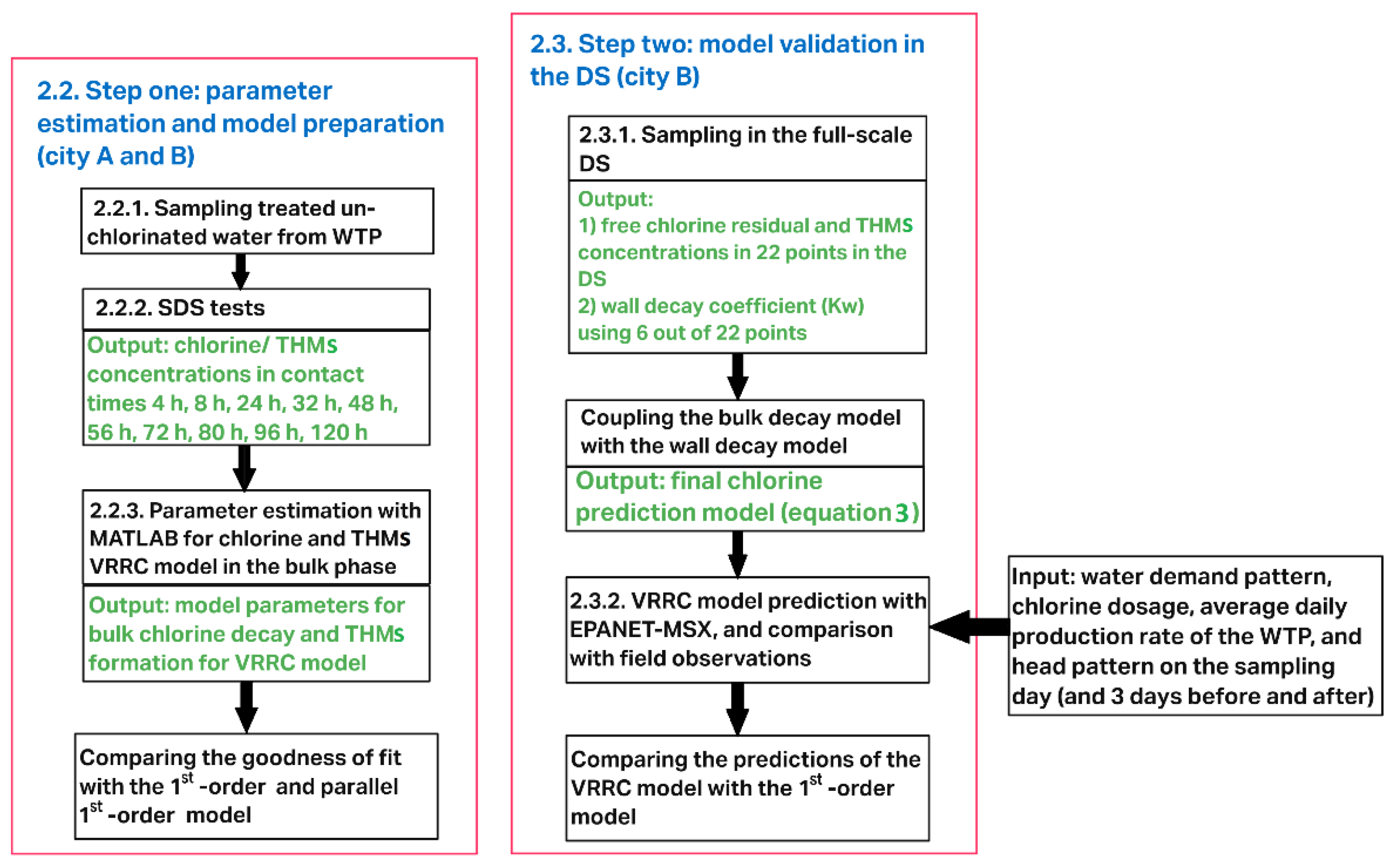
The procedure for predicting chlorine and THMs in the DS is divided into two main steps. Step one involves sampling at the WTP, performing simulated distribution system (SDS) tests in the lab, and using the lab results to estimate the model parameters. Step two consists of applying the calibrated model to predict chlorine and THMs concentrations in the DS with EPANET-MSX [27] and comparing predictions with field measurements. The lab experiments in step one were performed using waters from two WTP/DS, one with moderate concentration of ammonia (city A) and the other with low ammonia (city B). Step two was only conducted in city B due to the higher number of available regulatory points (n = 22) for model validation. This allowed us to evaluate the model performance in different pipe diameters, water residence times, and flow conditions. The different steps for prediction in the DS are described below.
2.2. Step One: Parameter Estimation and Model Preparation
2.2.1. Sampling at WTP
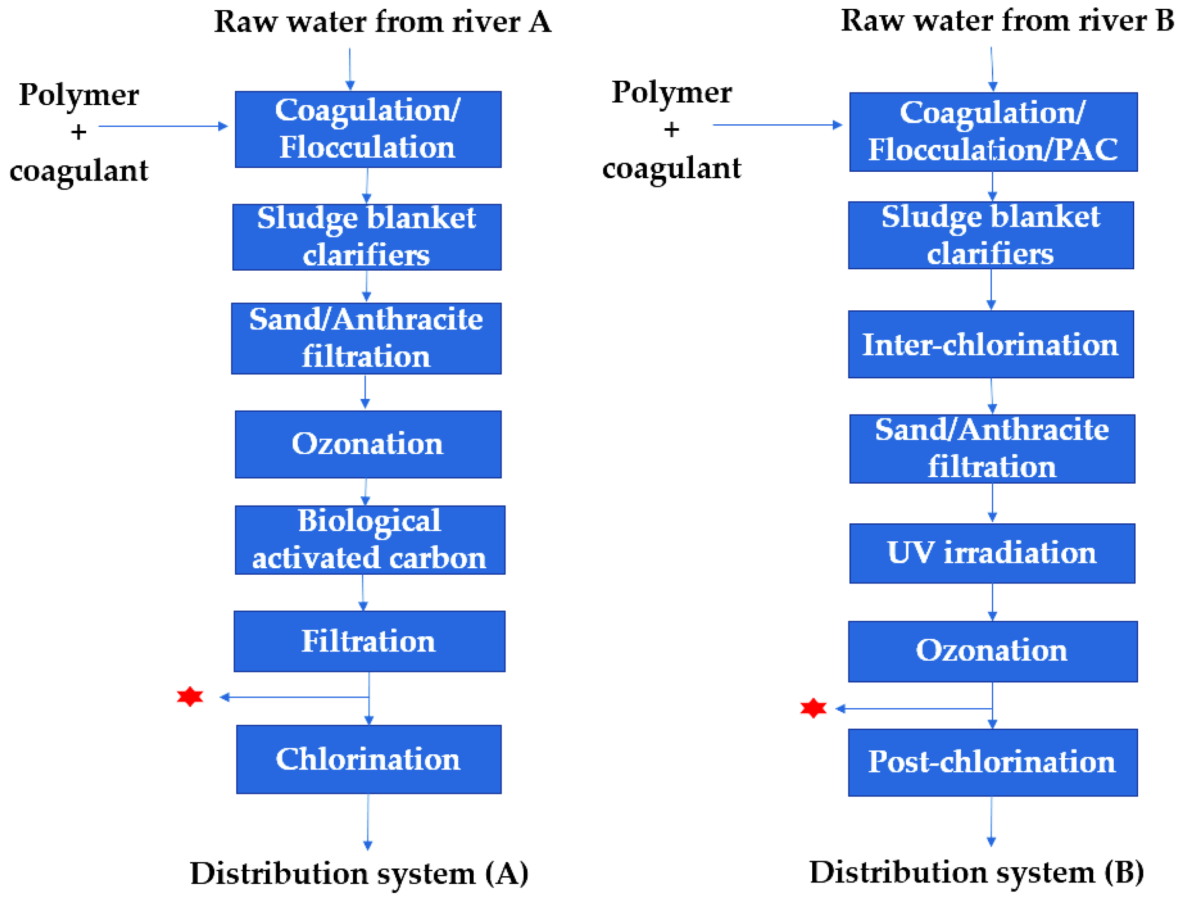
Water samples were collected from the WTPs (A and B). A different river water supplies each WTP. Three sampling campaigns were carried out in October 2020, March 2021, and October 2021. Therefore, filtered waters from each WTP exhibited different characteristics in terms of dissolved organic carbon (DOC), pH, temperature, and ammonia concentration. The treatment trains of each WTP are presented in Figure 1, and the red stars indicate the sampling locations for the chlorination experiments.
2.2.2. Simulated Distribution Systems (SDS) Assays
The SDS test is a standardized assay to simulate the chlorine demand originating from the bulk decay and formation of DBPs [28]. After chlorine injection, samples were transferred to 45-mL amber vials and incubated under the same temperature prevailing in the DS on the sampling day. Free chlorine residual was measured at multiple contact times (4 h, 8 h, 24 h, 32 h, 48 h, 56 h, 72 h, 80 h, 96 h, 120 h) based on the method 4500-Cl G of standard method for the examination of water and wastewater [28]. After each measurement, two 45 mL vials were quenched with ammonium sulfate, and the corresponding THMs concentrations were measured according to method EPA 524.2 (measurement of purgeable organic compounds in water by capillary column gas chromatography/mass spectrometry) [29]. All the analyses for chlorine and THMs were done in duplicates, and the coefficient of variance (CV) was calculated.
2.2.3. VRRC Model Parameters Estimation
The parameter estimation for chlorine and THMs models was performed using MATLAB R2019b (nonlinear differential equation curve fitting). The goodness of fit, including R-squared (R2), root mean square error (RMSE), and probability value (p-value), was calculated using the curve fitting toolbox of MATLAB (cftool 3.5.10).
- VRRC-chlorine model
Equation (1) presents the VRRC model for free chlorine prediction.
In this model, , expressed in mg/L, is the free chlorine concentration and is the chlorine demand in mg/L and is expressed as applied dosage . , the maximum chlorine demand (mg/L), is obtained based on the standard method [28] under specific conditions (pH = , temperature = , and a free chlorine residual 3–5 mg/L after 7 days). Finally, and are model parameters and are specific to physicochemical characteristics of water, mainly the NOM [12]. After finding the optimum parameters, the goodness of fit was compared to the 1st-order model [30], and the parallel 1st-order model [31].
- VRRC-THMs model
The VRRC-THMs model by Hua [26] needs a multi-step process for parameter estimation by first calibrating the model parameters based on trichloromethane formation, and then using a bromide substitution factor to estimate the total THMs formation. To reduce the model’s complexity and predict total THMs in one step, the original model was modified, and the final model is presented in Equation (2).
In this equation, M and N are model parameters describing the THMs formation rate, where M is expressed in and N is unitless. These parameters remain constant during the water travel time in the network. is the concentration of free chlorine at each time, and is the formed THMs at each time (, which equals . Finally, represents the maximum total THMs formation potential ( corresponding to the maximum chlorine demand obtained in the previous step. After estimating the model parameters, the model fit was compared to the 1st-order THMs model’s prediction by Clark [19]. The 1st-order THMs model is presented in Equation (S1) in the Supplementary Material, and Figure S1 shows the relationship between 1st-order chlorine and THMs concentrations for the estimation of THMs yield coefficient.
2.3. Step Two: Model Prediction and Validation
2.3.1. Sampling in Full-Scale DS
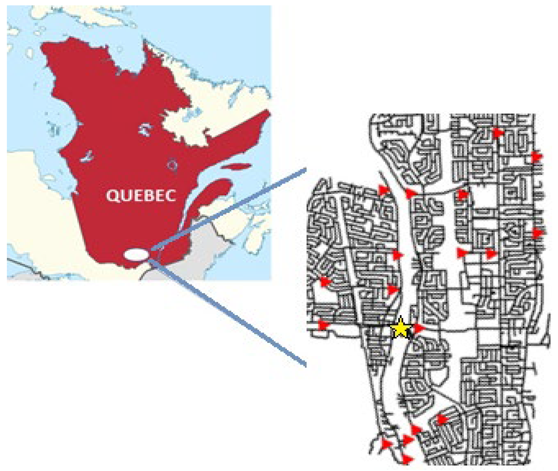
City B has an average annual production rate of 28,800 m3/day, and its EPANET network model includes approximately 2000 pipes and 1500 nodes. The average operating pressure of the network is 500 kPa. The pipe diameters range from 150 mm in secondary pipes to 600 mm in distribution mains. The pipe materials range from stainless steel for the pipes leaving the WTP, concrete for the distribution mains, cast iron for the secondary pipes, and PVC for most smaller diameter pipes. There are in total 22 regulatory control points in the network. The sampling points are in commercial areas, e.g., gas stations and commercial buildings. All samples were taken from the indoor consumer taps. The taps were left open for two minutes before collecting the samples. The precision of the chlorine measurement (Hach pocket colorimeterTM II, Saint-Laurent, Montreal, QC, Canada) was and for THMs, the quantification limit of the gas chromatography (Agilent Technologies 7890B gas chromatograph, Saint-Laurent, Montreal, QC, Canada) was between depending on the type of THMs. Therefore, to evaluate the goodness of our predictions, a target of prediction error for chlorine and prediction error for the THMs was considered acceptable. A segment of the overall layout of the city’s DS and the sampling points are presented in Figure 2. Predictions of free chlorine concentrations were carried out in two seasons, Spring (March) when the water temperature was 4 and Autumn (October) when the water temperature was 17.
2.3.2. VRRC Model Prediction and Comparison with Field Observations
Chlorine consumption in a DS originates from the bulk decay and wall decay [18,32]. The VRRC model predicts bulk decay only, and to use the model in a real-scale DS, a 1st-order wall decay model by Rossman, Clark [33] was used in conjunction with the VRRC model. The supplementary material explains the wall decay model in Equations (S2) and (S3). The overall chlorine decay equation composed of the bulk decay and the wall decay equation is presented in Equation (3).
In this equation, is the constant wall reaction rate with a unit of length per time and is the mass transfer coefficient (length/time), R is the pipe radius (length) and is the concentration of chlorine in the pipes (mg/L) [34]. The was estimated using 6 out of 22 data points with the aim of minimizing the RMSE between the predicted and the observed chlorine residuals. Then, the estimated was used for prediction of the 16 remaining points in the network. More details about estimation of and are provided in the Supplementary Material (part B).
Modeling chlorine residual and THMs in the DS was conducted with the EPANET-MSX version 1.1.00 The DS of the city had been previously modeled with EPANET 2.0 and the daily water production pattern of the WTP was used as the water demand pattern of all the network nodes (the pattern is provided in Figure S2 in the Supplementary Material). The demand patterns of days before and after the sampling were checked to ensure there were no anomalies around the sampling day that could impact our results, and no anomalies were found. The hourly head pattern of the plant was also applied to EPANET. The simulation time was extended to five days to stabilize the water quality model [27], and the results on the fifth day of the simulation were reported.
To compare predictions and observations, the sampling time for each node was identified first. For example, if the field observation was done at 10 a.m., the simulation results at 10 a.m. of the fifth day of simulation was identified. Finally, the predictions were compared to the 1st-order model for chlorine and THMs. The overall methodological approach of the study is summarized in Figure 3.
3. Results and Discussion
3.1. Parameter Estimation for the VRCC Model
Table 1 shows the characteristics of each water sample including DOC, ammonia concentration, pH, applied dosage in the lab, and the standard deviations for each parameter. Sampling from the plant of city A was carried out in late October 2020 when the water temperature was 10. At this period of the year, only partial nitrification was achieved in the biological filters [35], which explains the presence of ammonia in water.
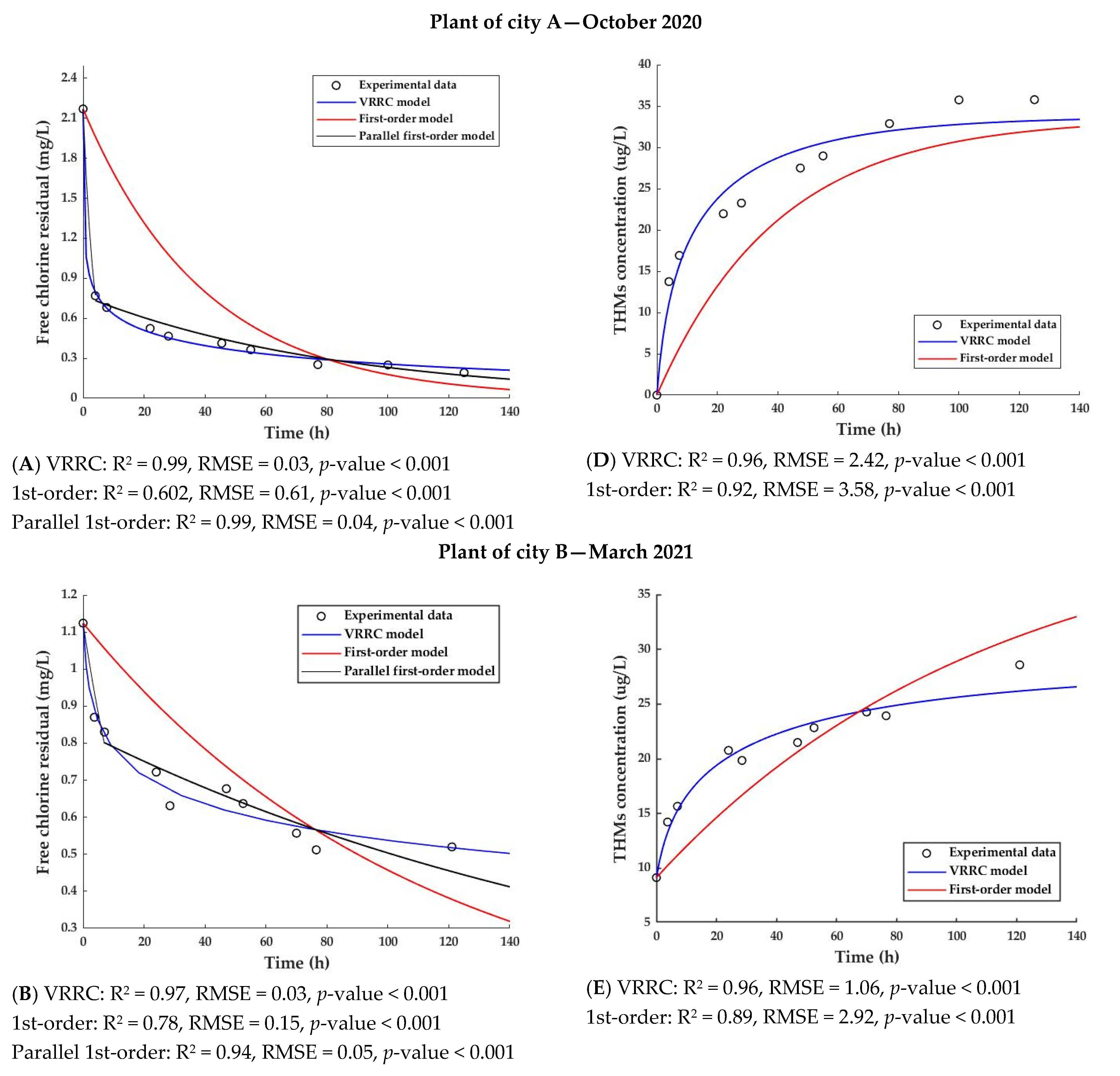
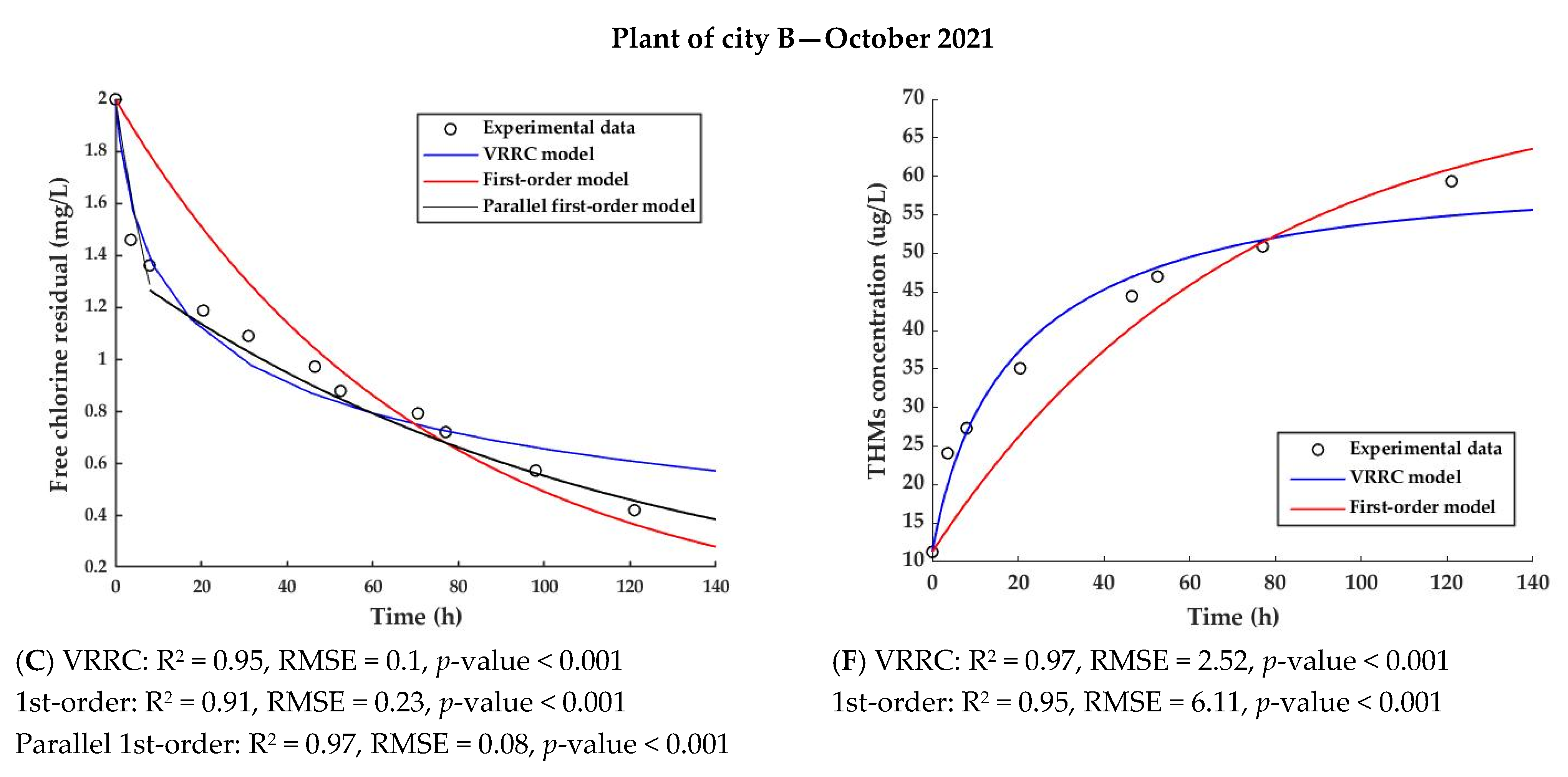
The predictions of the VRRC model for bulk chlorine decay and THMs formation were estimated with a CV less than 4% for Chlorine and CV less than 4.5% for THMs measurements. The results, including the curve fitting and the goodness of fit (R2, RMSE, and p-value) for each test, are presented in Figure 4.
As it can be seen in Figure 4A, the initial chlorine demand in the first few hours of the experiment was very high. This was due to the rapid reaction of free chlorine with ammonia. In this test, 69% of chlorine was consumed in the first 7.5 h of the experiment, reaching 91% after 125 h. Because of this significant decay rate in the initial stages of the reaction, the 1st-order model provided a poor fit to the experimental data. While the parallel 1st-order model fit was comparable to that of VRRC, it required finding the proper contact time for separating the slow reaction phase from the fast phase. Then, the model had to be recalibrated at the end of the slow phase, and the coefficient would change. In contrast to the parallel 1st-order model, VRRC model could predict chlorine decay with only one set of parameters for the whole test duration without recalibration. Moreover, VRRC coefficients are independent of the applied dosage. This means that under variable dosage of the treatment plant, we can still use the same parameters, whereas the parallel 1st-order model would need recalibration.
Regarding plant of city B (Figure 4B,C), the chlorine decay rate was more stable as compared to city A due to (1) negligible concentration of ammonia in water, (2) lower DOC concentration (1.68 in city B compared to 2.1 in city A), and (3) the intermediate chlorination performed before the filtration process that reduced the initial chlorine demand. The VRRC-chlorine model provided a better fit than the 1st-order model, and the parallel 1st-order model fit was equally good. The goodness of fit statistics also showed better fit by VRRC compared to the 1st-order model, and comparable to the parallel 1st-order model.
THMs prediction results are presented in Figure 4D–F. In presence of ammonia (city A plant), VRRC showed a better fit compared to the 1st-order THMs model. As opposed to the chlorine decay rate, which had a drastic decline in the first few hours, the THMs formation rate was steadier given that the ammonia-Cl2 reaction does not lead to the formation of THMs. In WTP of city B, where the ammonia concentration was low, VRRC provided a better fit than the 1st-order model. The goodness of fit statistics provided below each figure show that VRRC yielded a higher R2 and a lower RMSE in all three waters, indicating that the fit was improved compared to the 1st-order THMs model.
3.2. Predicting Free Chlorine and THMs in the DS
3.2.1. Free Chlorine Prediction
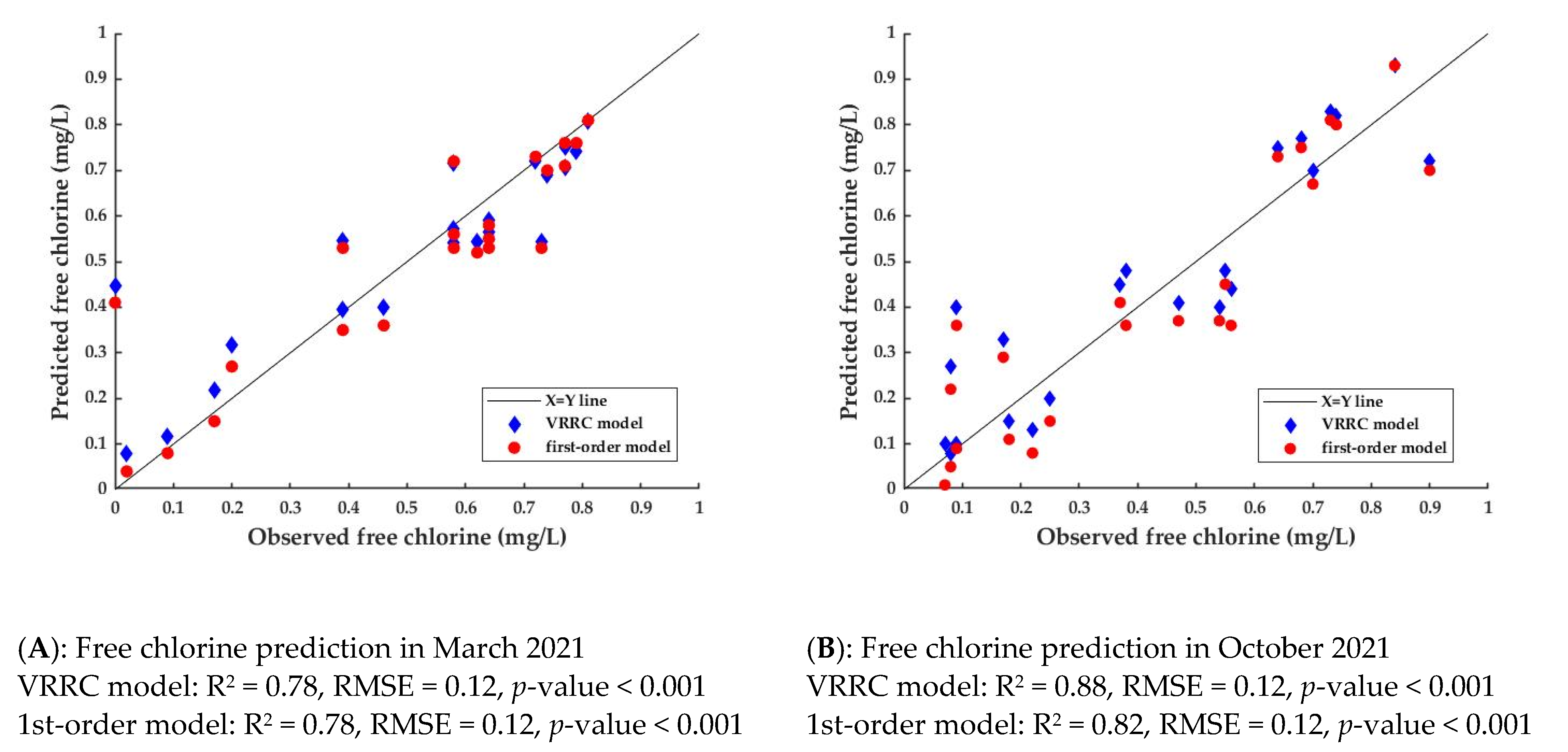
Figure 5 presents the predicted free chlorine versus the observed values in both seasons. The optimized for the studied network was 0.04 m/day for March (DS water temperature = 4) and 0.12 m/day for October (DS water temperature = 17). The faster kinetics and higher in higher temperatures have been previously reported in the literature [36,37,38,39]. Prediction of free chlorine in city B met our target accuracy in both Spring and Fall in most of the sampling points. This figure also shows the goodness of fit statistics for both VRRC and the 1st-order models (R2, RMSE, and p-value). Table S1 in the supplementary materials presents the sampling points’ diameters, observed nodal residual chlorine, and VRRC prediction results in both seasons.
In Spring, the target precision of was met in 77% of the sampling points (17 out of 22) with both VRRC and the 1st-order model. The prediction errors were higher than in points N4, N11, N13, N20, and N22. All these nodes were located on small diameter pipes (150–250 mm). In smaller diameters, the ratio of surface to volume increases, which in turn increases the interaction of pipe walls and biofilm material with water. This high interaction increases the pipe wall decay coefficient locally. Fisher, Kastl [18] have previously shown that using a single value for the whole network will generally lead to better predictions in larger pipes and higher errors in smaller pipes. Based on our results, using two different values, one for the transport mains (larger pipes) and one for the distribution lines (smaller pipes), could improve the prediction results. Another error source was that Nodes N13, and N20 were on network dead ends, and N4 was on the extremities and very close to a dead end. The hydraulics of these points are usually poorly described in hydraulic models like EPANET, and the water stagnation is usually higher than the calculations of EPANET which leads to an increased prediction error [33].
Prediction of free chlorine in October met the precision target at 73% of the points (16 out of 22 points) with the VRRC model and 68% of the points (15 out of 22) with the 1st-order model. Points N7, N12, N13, N16, N21, and N22, had prediction errors higher than . The diameters of pipes in all these points were between 150–200 mm, which led to a higher prediction error because of the wall decay effect. In addition to having a small diameter, Node N13 was at a dead end, which increased the prediction error.
In addition to the above reasons for the prediction error, the samples were collected from non-residential buildings during the COVID pandemic. This situation may have modified the water demand allocation in the DS, which was not well described in the hydraulic simulation. Finally, the RMSE in both seasons was 0.12, close to our precision target of maximum error. The overall prediction was deemed acceptable considering five dead ends and the pandemic contextual factors.
To improve prediction, we can allocate specific demand patterns to the nodes on the distribution pipes. Blokker, Vreeburg [40] found that using a stochastic demand with a smaller hydraulic timestep (one minute instead of one hour used in this work) will reduce the prediction error. A bottom-up approach with a small timestep can describe the household demand variations more realistically. This will lead to a more realistic calculation of RT at each node and lower prediction errors.
3.2.2. THMs Prediction
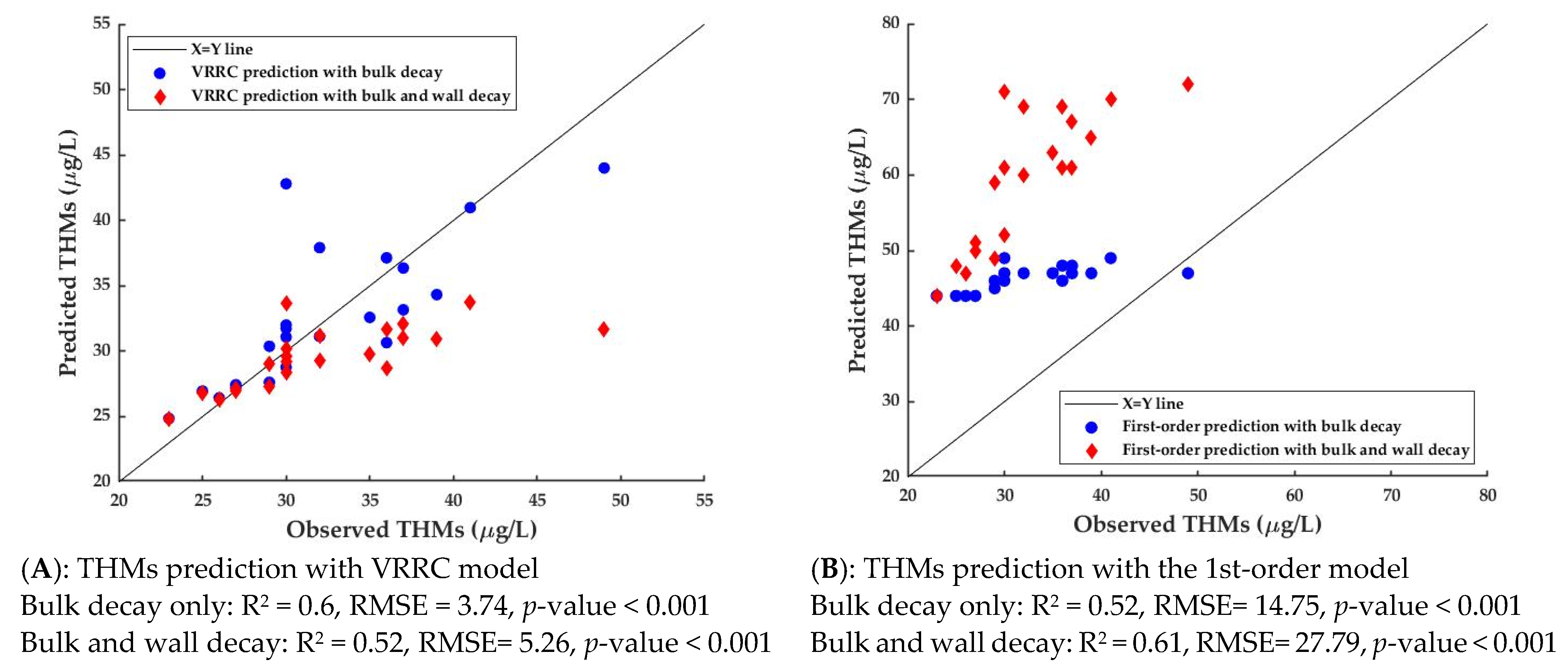
The prediction results for the VRRC and the 1st-order models and the goodness of fit statistics are presented in Figure 6. THMs prediction in the DS was performed in two ways: (1) considering the bulk chlorine decay only, and (2) considering both bulk and wall decay. For the VRRC model, predicting with the bulk decay met the target precision of in 91% (20 out of 22) of the locations with an RMSE = 3.7 . However, considering both bulk and wall decay reduced the performance as our target was met in 73% (16 out of 22) of the locations with an RMSE = 5.3 . This result suggests that the organic matter adsorbed on pipe walls and deposits did not acta as a significant source of DBPs precursors. Koch, Krasner [41] have also found that THM-SDS values obtained in the lab correlate perfectly with field measurements. Since THMs formation is influenced by free chlorine reconcentration, a conclusion from this result in the studied network could be that the dominant source of chlorine prediction error (especially in the smaller diameter pipes) is not the wall decay effect but rather due to the lack of specific demand patterns (which lead to RT calculation errors). The fact that most of the smaller diameter pipes in this DS are made of PVC (have lower ) supports this assumption. THMs predictions with the 1st-order model considering the bulk decay met the target precision only in 1 out of 22 locations (Figure 6B). Considering both wall and bulk decay did not help meeting our target as the prediction error increased substantially. The lack of fit of the 1st-order model is due to an overestimation of THMs given that not all chlorine decay led to the formation of THMs. Table S2 presents the nodal THMs concentrations measured in the field, their corresponding pipe diameter, THMs prediction with VRRC using bulk decay, and their absolute prediction errors.
4. Conclusions
The VRRC model was an effective tool for predicting chlorine and THMs in the lab and in a full-scale DS. Free chlorine prediction in the presence of ammonia is challenging for most models, given the significant change in chlorine decay rate. VRRC successfully predicted chlorine and THMs in the presence of ammonia without recalibration or the need to change the parameters as opposed to the 1st-order and the parallel 1st-order model. Prediction of free chlorine in the DS was performed in two seasons to test the model applicability under seasonal changes in water quality (temperature, DOC, dosage, ). The free chlorine predictions with VRRC (in low-ammonia concentrations) were comparable and slightly better than the 1st-order model’s prediction. Accurate prediction of chlorine in the full-scale DS is essential in meeting the minimum set points set by several jurisdictions. Another advantage of using the VRRC in full-scale applications is its constant model coefficients under variable dosage and rechlorination.
THMs prediction in the DS was successfully achieved with the VRRC, while the 1st-order model predictions did not meet our prediction target (5 µg/L). An advantage of this approach was that a precise THMs prediction was achieved using only lab-scale results without calibration of the model in the network. This ability especially becomes important to utilities under global change in drinking water quality. Under abrupt or seasonal changes in source water quality, the risk of THMs non-compliance in the DS may increase. Meeting DBPs regulatory standards is one of the utilities’ most important concerns, especially under changing climatic conditions. A simple tool to predict the possibility of THMs non-compliance, especially in the extremities and riskier locations, can be an asset to utilities. Predicting THMs non-compliance from the treatment plant will also enable utilities to test the efficiency of different strategies for reducing THMs in the DS.
The chlorine and THMs predictions with VRRC were validated in various DS locations with different physical and hydraulic conditions, from the treatment plant to the DS extremities. As a result, this model can be used to predict chlorine/THMs in the entire DS of the city. The simplicity of our approach makes it easily accessible to small utilities with limited resources. Under changing conditions, our system can be used to assess the risk of chlorine/THMs non-compliance under different climatic scenarios. The results can be the starting point for decision-making on mitigation strategies to avoid the negative consequences of adverse climatic events on public health.
Supplementary Materials
The following supporting information can be downloaded at: https://www.mdpi.com/article/10.3390/w14223685/s1, Figure S1: Relationship between THMs and 1st-order chlorine decay for estimating the THMs yield coefficient, Figure S2: Hourly water demand patterns for March and October 2021 in city B, Table S1: Free chlorine prediction results in the field including the pipe diameter, free chlorine residual (observed and predicted), and absolute prediction error, Table S2: THMs prediction results in the DS including the pipe diameter, THMs concentrations (observed and predicted), and absolute prediction error.
Author Contributions
Conceptualization and methodology, F.A., F.B., B.B. and M.P.; software, F.A. and F.H.; validation of the model, F.A.; sampling and data collection, F.A.; writing—original draft preparation, F.A.; writing—review and editing, all authors; visualization, F.A.; supervision, F.B., B.B. and M.P. All authors have read and agreed to the published version of the manuscript.
Funding
This research was funded by the Discovery Grant from the Natural Sciences and Engineering Research Council of Canada (NSERC) of the last author (F.B.) and Polytechnique Montreal’s partial doctoral training support scholarships (F.B.), as well as by the Industrial Chair on Drinking Water of B.B. and M.P.
Acknowledgments
The authors would like to thank the participating utilities for providing administrative and technical support, and the lab personnel of industrial chair on drinking water in Polytechnique Montréal for their technical support and guidance during this project.
Conflicts of Interest
The authors declare no conflict of interest. The funders had no role in the design of the study; in the collection, analyses, or interpretation of data; in the writing of the manuscript, or in the decision to publish the results.
References
- Méité, L.; Fotsing, M.; Barbeau, B. Efficacy of ozone to reduce chlorinated disinfection by-products in Quebec (Canada) drinking water facilities. Ozone Sci. Eng. 2015, 37, 294–305. [Google Scholar] [CrossRef]
- Jonkergouw, P.M.R.; Khu, S.-T.; Savic, D.A.; Zhong, D.; Hou, X.Q.; Zhao, H.-B. A Variable Rate Coefficient Chlorine Decay Model. Environ. Sci. Technol. 2009, 43, 408–414. [Google Scholar] [CrossRef] [PubMed]
- Code of Federal Regulations (CFR). 40 CFR 141.72. National Primary Drinking Water Regulations, Subpart H—Filtration and Disinfection, Disinfection; U.S. Government: Washington, DC, USA, 2010; pp. 456–458. Available online: https://www.ecfr.gov/current/title-40/chapter-I/subchapter-D/part-141/subpart-H (accessed on 20 October 2022).
- Walski, T. Raising the bar on disinfectant residuals. World Water Mag. 2019, 42, 34–35. [Google Scholar]
- Rossman, L.A.; Brown, R.A.; Singer, P.C.; Nuckols, J.R. DBP formation kinetics in a simulated distribution system. Water Res. 2001, 35, 3483–3489. [Google Scholar] [CrossRef]
- Simard, A.; Pelletier, G.; Rodriguez, M. Water residence time in a distribution system and its impact on disinfectant residuals and trihalomethanes. J. Water Supply Res. Technol. 2011, 60, 375–390. [Google Scholar] [CrossRef]
- Sérodes, J.-B.; Rodriguez, M.J.; Li, H.; Bouchard, C. Occurrence of THMs and HAAs in experimental chlorinated waters of the Quebec City area (Canada). Chemosphere 2003, 51, 253–263. [Google Scholar] [CrossRef]
- Chhipi-Shrestha, G.; Rodriguez, M.; Sadiq, R. Unregulated disinfection By-products in drinking water in Quebec: A meta analysis. J. Environ. Manag. 2018, 223, 984–1000. [Google Scholar] [CrossRef]
- US Envionmental Protection Agency (USEPA). Stage 2 Disinfectants and Disinfection Byproducts Rule: A Quick Reference Guide For Schedule 4 Systems; USEPA: Cincinnati, OH, USA, 2006. Available online: https://nepis.epa.gov/Exe/ZyPDF.cgi?Dockey=P100A2D8.txt (accessed on 20 October 2022).
- US Envionmental Protection Agency. Comprehensive Disinfectants and Disinfection Byproducts Rules (Stage 1 and Stage 2): Quick Reference Guide; Systems DWRfSaPW; USEPA: Cincinnati, OH, USA, 2010. Available online: https://www.epa.gov/dwreginfo/stage-1-and-stage-2-disinfectants-and-disinfection-byproducts-rules (accessed on 20 October 2022).
- Tryby, M.E.; Boccelli, D.L.; Koechling, M.T.; Uber, J.G.; Summers, R.S.; Rossman, L.A. Booster chlorination for managing disinfectant residuals. J. Am. Water Work. Assoc. 1999, 91, 95–108. [Google Scholar] [CrossRef]
- Hua, P.; Vasyukova, E.; Uhl, W. A variable reaction rate model for chlorine decay in drinking water due to the reaction with dissolved organic matter. Water Res. 2015, 75, 109–122. [Google Scholar] [CrossRef]
- Fisher, I.; Kastl, G.; Sathasivan, A. Evaluation of suitable chlorine bulk-decay models for water distribution systems. Water Res. 2011, 45, 4896–4908. [Google Scholar] [CrossRef]
- Meng, F.; Liu, S.; Ostfeld, A.; Chen, C.; Burchard-Levine, A. A deterministic approach for optimization of booster disinfection placement and operation for a water distribution system in Beijing. J. Hydroinformatics 2013, 15, 1042–1058. [Google Scholar] [CrossRef]
- Al Heboos, S.; Licskó, I. Application and comparison of two chlorine decay models for predicting bulk chlorine residuals. Period. Polytech. Civ. Eng. 2017, 61, 7–13. [Google Scholar] [CrossRef] [Green Version]
- Hallam, N.; West, J.; Forster, C.; Powell, J.; Spencer, I. The decay of chlorine associated with the pipe wall in water distribution systems. Water Res. 2002, 36, 3479–3488. [Google Scholar] [CrossRef]
- García-Ávila, F.; Avilés-Añazco, A.; Ordoñez-Jara, J.; Guanuchi-Quezada, C.; del Pino, L.F.; Ramos-Fernández, L. Modeling of residual chlorine in a drinking water network in times of pandemic of the SARS-CoV-2 (COVID-19). Sustain. Environ. Res. 2021, 31, 1–15. [Google Scholar] [CrossRef]
- Fisher, I.; Kastl, G.; Sathasivan, A. New model of chlorine-wall reaction for simulating chlorine concentration in drinking water distribution systems. Water Res. 2017, 125, 427–437. [Google Scholar] [CrossRef]
- Clark, R.M. Chlorine Demand and TTHM Formation Kinetics: A Second-Order Model. J. Environ. Eng. 1998, 124, 16–24. [Google Scholar] [CrossRef]
- Boccelli, D.L.; Tryby, M.E.; Uber, J.G.; Summers, R. A reactive species model for chlorine decay and THM formation under rechlorination conditions. Water Res. 2003, 37, 2654–2666. [Google Scholar] [CrossRef]
- Gang, D.; Clevenger, T.E.; Banerji, S.K. Relationship of chlorine decay and THMs formation to NOM size. J. Hazard. Mater. 2003, 96, 1–12. [Google Scholar] [CrossRef]
- Deborde, M.; von Gunten, U. Reactions of chlorine with inorganic and organic compounds during water treatment—Kinetics and mechanisms: A critical review. Water Res. 2008, 42, 13–51. [Google Scholar] [CrossRef]
- Yang, X.; Shang, C.; Lee, W.; Westerhoff, P.; Fan, C. Correlations between organic matter properties and DBP formation during chloramination. Water Res. 2008, 42, 2329–2339. [Google Scholar] [CrossRef]
- Zhang, X.-L.; Yang, H.-W.; Wang, X.-M.; Fu, J.; Xie, Y.F. Formation of disinfection by-products: Effect of temperature and kinetic modeling. Chemosphere 2013, 90, 634–639. [Google Scholar] [CrossRef] [PubMed]
- Gallard, H.; von Gunten, U. Chlorination of phenols: Kinetics and formation of chloroform. Environ. Sci. Technol. 2002, 36, 884–890. [Google Scholar] [CrossRef] [PubMed]
- Hua, P. Variable Reaction Rate Models for Chlorine Decay and Trihalomethanes Formation in Drinking and Swimming Pool Waters; Technische Universität: Dresden, Germany, 2016; Available online: https://d-nb.info/1226430732/3 (accessed on 20 October 2022).
- Shang, F.; Uber, J.G.; Rossman, L.A.; Janke, R. EPANET Multi-Species Extension User’s Manual; Risk Reduction Engineering Laboratory, US Environmental Protection Agency: Cincinnati, OH, USA, 2008. [Google Scholar]
- American Public Health Association (APHA); American Water Works Association (AWWA); Water Environment Federation (WEF). Standard Methods for the Examination of Water and Wastewater; American Public Health Association: Washington, DC, USA, 2012. [Google Scholar]
- United States Envionmental Protection Agency (USEPA). Method 524.2. Measurement of Purgeable Organic Compounds in Water by Capillary Column Gas Chromatography/Mass Spectrometry; USEPA: Cincinnati, OH, USA, 1992; p. 43. Available online: https://settek.com/EPA-Method-524-2/ (accessed on 20 October 2022).
- Vasconcelos, J.J.; Rossman, L.A.; Grayman, W.M.; Boulos, P.F.; Clark, R.M. Kinetics of chlorine decay. J. Am. Water Work. Assoc. 1997, 89, 54–65. [Google Scholar] [CrossRef]
- Powell, J.C.; West, J.R.; Hallam, N.B.; Forster, C.F.; Simms, J. Performance of Various Kinetic Models for Chlorine Decay. J. Water Resour. Plan. Manag. 2000, 126, 13–20. [Google Scholar] [CrossRef]
- Shang, F.; Uber, J.G. Calibrating Pipe Wall Demand Coefficient for Chlorine Decay in Water Distribution System. J. Water Resour. Plan. Manag. 2007, 133, 363–371. [Google Scholar] [CrossRef]
- Rossman, L.A.; Clark, R.M.; Grayman, W.M. Modeling chlorine residuals in drinking-water distribution systems. J. Environ. Eng. 1994, 120, 803–820. [Google Scholar] [CrossRef]
- Rossman, L.A. EPANET Users Manual; USEPA: Cincinnati, OH, USA, 1994. Available online: https://nepis.epa.gov/Exe/ZyPURL.cgi?Dockey=3000349Y.TXT (accessed on 20 October 2022).
- Liu, Z.; Lompe, K.M.; Mohseni, M.; Bérubé, P.R.; Sauvé, S.; Barbeau, B. Biological ion exchange as an alternative to biological activated carbon for drinking water treatment. Water Res. 2020, 168, 115148. [Google Scholar] [CrossRef]
- McNeill, L.S.; Edwards, M. The importance of temperature in assessing iron pipe corrosion in water distribution systems. Environ. Monit. Assess. 2002, 77, 229–242. [Google Scholar] [CrossRef]
- Volk, C.; Dundore, E.; Schiermann, J.; Lechevallier, M. Practical evaluation of iron corrosion control in a drinking water distribution system. Water Res. 2000, 34, 1967–1974. [Google Scholar] [CrossRef]
- Kahil, M.A. Application of First Order Kinetics for Modeling Chlorine Decay in Water Networks. Int. J. Sci. Eng. Res. 2016, 7, 331–336. [Google Scholar]
- McGrath, J.; Maleki, M.; Bouchard, C.; Pelletier, G.; Rodriguez, M.J. Bulk and pipe wall chlorine degradation kinetics in three water distribution systems. Urban Water J. 2021, 18, 512–521. [Google Scholar] [CrossRef]
- Blokker, E.J.M.; Vreeburg, J.H.G.; Buchberger, S.G.; van Dijk, J.C. Importance of demand modelling in network water quality models: A review. Drink. Water Eng. Sci. 2008, 1, 27–38. [Google Scholar] [CrossRef]
- Koch, B.; Krasner, S.W.; Sclimenti, M.J.; Schimpff, W.K. Predicting the Formation of DBPs by the Simulated Distribution System. J. Am. Water Work. Assoc. 1991, 83, 62–70. [Google Scholar] [CrossRef]
Figure 1.
Schematic of the treatment chains for WTPs of City A and City B. The stars indicate the location of the sampling point in each plant.
Figure 1.
Schematic of the treatment chains for WTPs of City A and City B. The stars indicate the location of the sampling point in each plant.

Figure 2.
Layout of the DS of city B in southern Quebec (the image is neither showing the whole network nor all the 22 sampling points for model validation). The locations of the sampling points are indicated with red triangles, and the WTP is marked with a yellow star.
Figure 2.
Layout of the DS of city B in southern Quebec (the image is neither showing the whole network nor all the 22 sampling points for model validation). The locations of the sampling points are indicated with red triangles, and the WTP is marked with a yellow star.

Figure 3.
Overall methodological approach for parameter estimation and model validation in the DS.

Figure 4.
Curve fitting results and goodness of fit for chlorine and THMs; comparison with the 1st-order and the parallel 1st-order model.
Figure 4.
Curve fitting results and goodness of fit for chlorine and THMs; comparison with the 1st-order and the parallel 1st-order model.


Figure 5.
Free chlorine prediction results in the DS of city B using the VRRC model compared to the 1st-order model.
Figure 5.
Free chlorine prediction results in the DS of city B using the VRRC model compared to the 1st-order model.

Figure 6.
THMs prediction results and goodness of prediction in the DS; comparison between the VRRC and the 1st-order models.
Figure 6.
THMs prediction results and goodness of prediction in the DS; comparison between the VRRC and the 1st-order models.


Table 1.
Characteristics of the water samples (average standard deviation) taken from cities A and B.
Table 1.
Characteristics of the water samples (average standard deviation) taken from cities A and B.
| Water Source | DS Temperature (°C) | Ammonia Concentration (μg N/L) | DOC (mg C/L) | pH | Applied Dosage in the Lab (mg Cl2/L) |
|---|---|---|---|---|---|
| City A WTP (October 2020) 1 sample tested | 10 | 91 ± 5 | 2.10.03 | 7.10.03 | 2.170.03 |
| City B WTP (March 2021) 2 samples tested | 4 | <5 | 1.520.04 | 7.840.03 | 1.120.009 |
| City B WTP (October 2021) 3 samples tested | 17 | <5 | 1.680.04 | 7.820.02 | 2.00 |
Publisher’s Note: MDPI stays neutral with regard to jurisdictional claims in published maps and institutional affiliations. |
© 2022 by the authors. Licensee MDPI, Basel, Switzerland. This article is an open access article distributed under the terms and conditions of the Creative Commons Attribution (CC BY) license (https://creativecommons.org/licenses/by/4.0/).
Share and Cite
MDPI and ACS Style
Absalan, F.; Hatam, F.; Barbeau, B.; Prévost, M.; Bichai, F. Predicting Chlorine and Trihalomethanes in a Full-Scale Water Distribution System under Changing Operating Conditions. Water 2022, 14, 3685. https://doi.org/10.3390/w14223685
AMA Style
Absalan F, Hatam F, Barbeau B, Prévost M, Bichai F. Predicting Chlorine and Trihalomethanes in a Full-Scale Water Distribution System under Changing Operating Conditions. Water. 2022; 14(22):3685. https://doi.org/10.3390/w14223685
Chicago/Turabian StyleAbsalan, Faezeh, Fatemeh Hatam, Benoit Barbeau, Michèle Prévost, and Françoise Bichai. 2022. "Predicting Chlorine and Trihalomethanes in a Full-Scale Water Distribution System under Changing Operating Conditions" Water 14, no. 22: 3685. https://doi.org/10.3390/w14223685
Note that from the first issue of 2016, this journal uses article numbers instead of page numbers. See further details here.