
Hazard Assessment of Potential Large-Scale Landslides in the Watershed of the Chenyulan River

1
Department of Landscape and Urban Design, Chaoyang University of Technology, Taichung 413310, Taiwan
2
Department of Construction Engineering, Chaoyang University of Technology, Taichung 413310, Taiwan
*
Author to whom correspondence should be addressed.
Water 2022, 14(22), 3692; https://doi.org/10.3390/w14223692
Submission received: 4 October 2022
/
Revised: 7 November 2022
/
Accepted: 10 November 2022
/
Published: 15 November 2022
(This article belongs to the Section Hydrology)
Abstract
:Taiwan’s mountains are steep, geologically dispersed, and their hillsides are over-utilized. Serious debris flow disasters are prone to happen whenever monsoons or typhoons bring a lot of rain. Typhoon Morakot’s large-scale landslide in 2009, which devastated half of Xiaolin Village and claimed around 500 lives, is one such instance. Large-scale landslides have the potential to seriously harm people, property, and the economy. Large-scale landslides were less frequent in the past, but they have recently increased in frequency. An important topic is how to avert disasters through efficient risk management. Eight influencing factors were chosen after multivariate analysis screening, including three terrestrial factors (total catchment area size, average catchment area slope, and total curvature), three material factors (stratum type, distance from fault, and average normalized-difference vegetation index prior to the event), and two trigger factors (maximum daily rainfall and maximum hourly rainfall). Our overall analysis’ accuracy rankings were as follows: neural network, 93.7%; logistic regression analysis, 92.2%; and discriminant analysis, 89%. The area under curve (AUC) values for the neural network (0.819), discriminant analysis (0.824), and logistic regression analysis (0.732) all demonstrated high discriminative abilities based on the receiver operating characteristic curve, indicating that all three of our models are adequate for this purpose. Large-scale debris flow disasters are more likely to happen when the catchment region’s total area, total curvature, and average slope are higher, according to a cluster study. These findings can help to decrease the effects of disasters of this kind by helping to create early warning systems.
1. Introduction
Taiwan is located in the Pacific Rim seismic zone, at the junction of the Philippine Sea plate and the Eurasian plate. Its total land area is about 36,000 km2, of which some two-thirds consists of mountain slopes. Most of its geology belongs to the tertiary or quaternary strata, which are relatively new and quite fragile. The significant erosion of riverbeds caused by the steep slopes and swift currents increases the likelihood of slope disasters such as landslides, debris flows, and landslides. In addition, Taiwan has a subtropical marine climate, with an average annual rainfall of up to 2500 mm, mostly concentrated in summer and autumn. Its rapid industrialization and associated increase in population density have led to the development of hillsides, which—where not carefully planned and executed—has led to a decline in their stability. Moreover, the increasingly extreme hydrological conditions associated with climate change, when coupled with the above-mentioned topographical and human factors, mean that the scale of slope disasters is trending upwards. Road damage in mountainous areas inevitably results from heavy rain and typhoons, and comes at a high cost in life and property. In the years since the “921 Jiji earthquake” of 1999 loosened topsoil, the area of Taiwan deemed to be landslide-prone nearly doubled, from 8110 to 15,977 hectares; and worse, the areas actually affected by landslides increased from 2535 to 25,845 hectares [1]. Among the large-scale mass movement disasters that have been more prevalent in Taiwan since 1999, the most serious was the destruction of Xiaolin Village, following deep damage to Xiandu Mountain caused by Typhoon Morakot. Since that incident, scholars and government agencies have devoted increasing attention to large-scale landslide events, but such research is challenging because actual cases are relatively rare. Therefore, this study explores methods of modeling such events using satellite images taken before and after previous ones, to serve the wider aim of creating an early warning system that will reduce the impact of these disasters.
Landslides can be defined in several ways: according to their mechanisms (Varnes, 1978; Santacana et al., 2003; Liu et al., 2009), their causes (Renwick et al., 1982), their depth (Fell et al., 2000; Santacana et al., 2003; Giannecchini, 2006; Japan Institute of Civil Engineering, 2008; Minami, 2010), and so on [2,3,4,5,6,7,8,9]. Chigira (2011) and National Science and Technology Center for Disaster Reduction (2015) both define large-scale landslides as those covering an area of more than 10 hectares, or that have a volume of greater than 100,000 m3, or a depth of more than 10 m; and these same characteristics are likely to render them fast-moving [10,11]. It takes a lot of time and effort to investigate tragedies on sloping land the traditional way, which involves sending inspectors there on foot. Consequently, really steep terrain in many alpine places is not actually examined. Telemetry photos are of tremendous use in disaster prevention on sloping ground because they can serve as the foundation for further study and analysis across a wide area. As a result, these photos serve as the major source of data for the current work, and correlational analysis is utilized to examine the impact of different conditions on how landslides develop. It is intended that the findings will give government agencies entrusted with decreasing the losses from such calamities a quick and simple reference.
2. Materials and Methods
2.1. Study Area
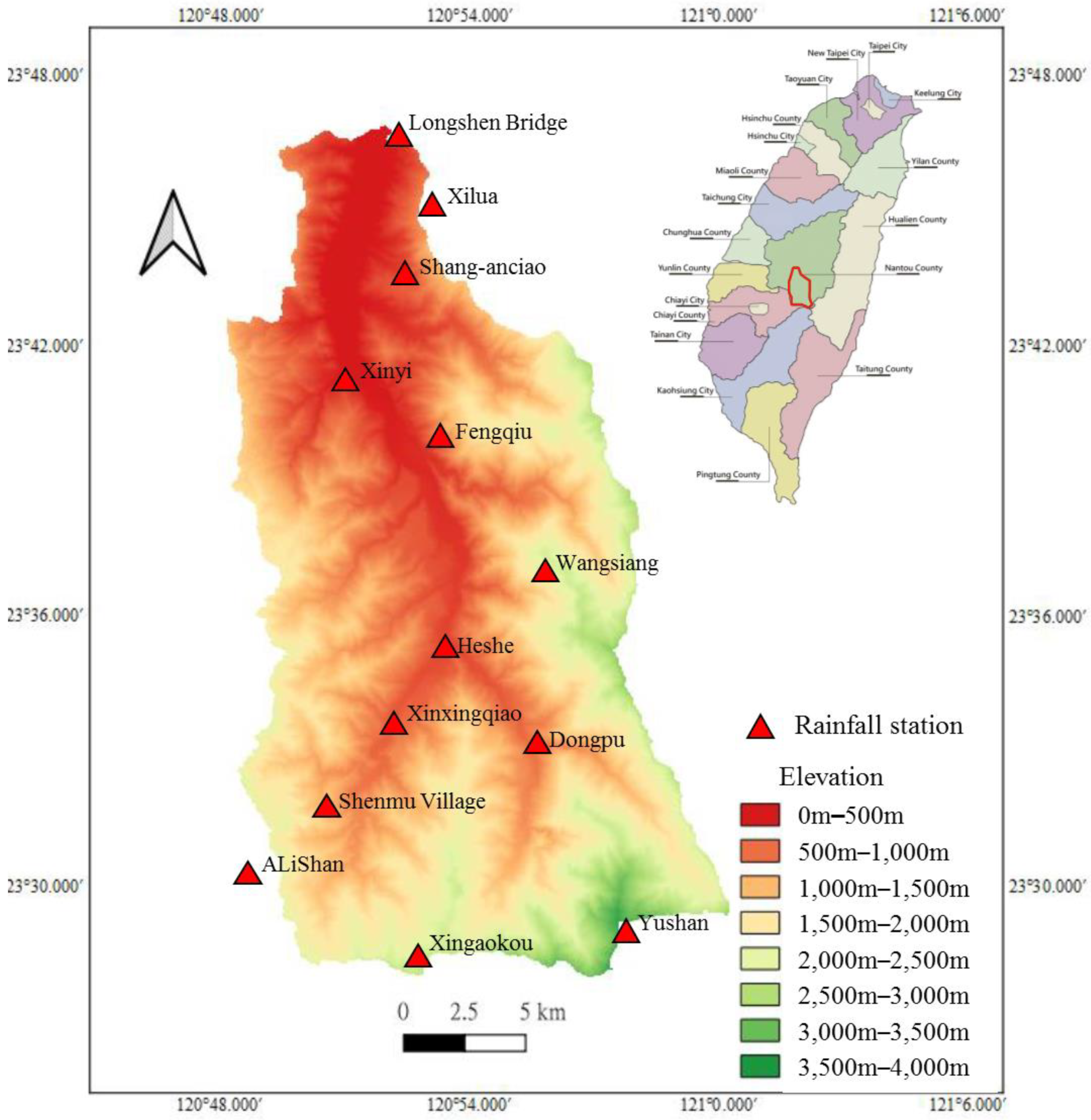
The study area is the Chenyoulan River, one of the important tributaries of the Zhuoshui River. The Chenyoulan runs through Xinyi Township, Shuili Township, and Lugu Township, all in Nantou County, between 120°47′ to 120°57′ east longitude and 23°26′ to 23°47′ north latitude (Figure 1). The terrain of this area is higher in the southeast and lower in the northwest, while the catchment area is narrow in the north and widens toward the south.
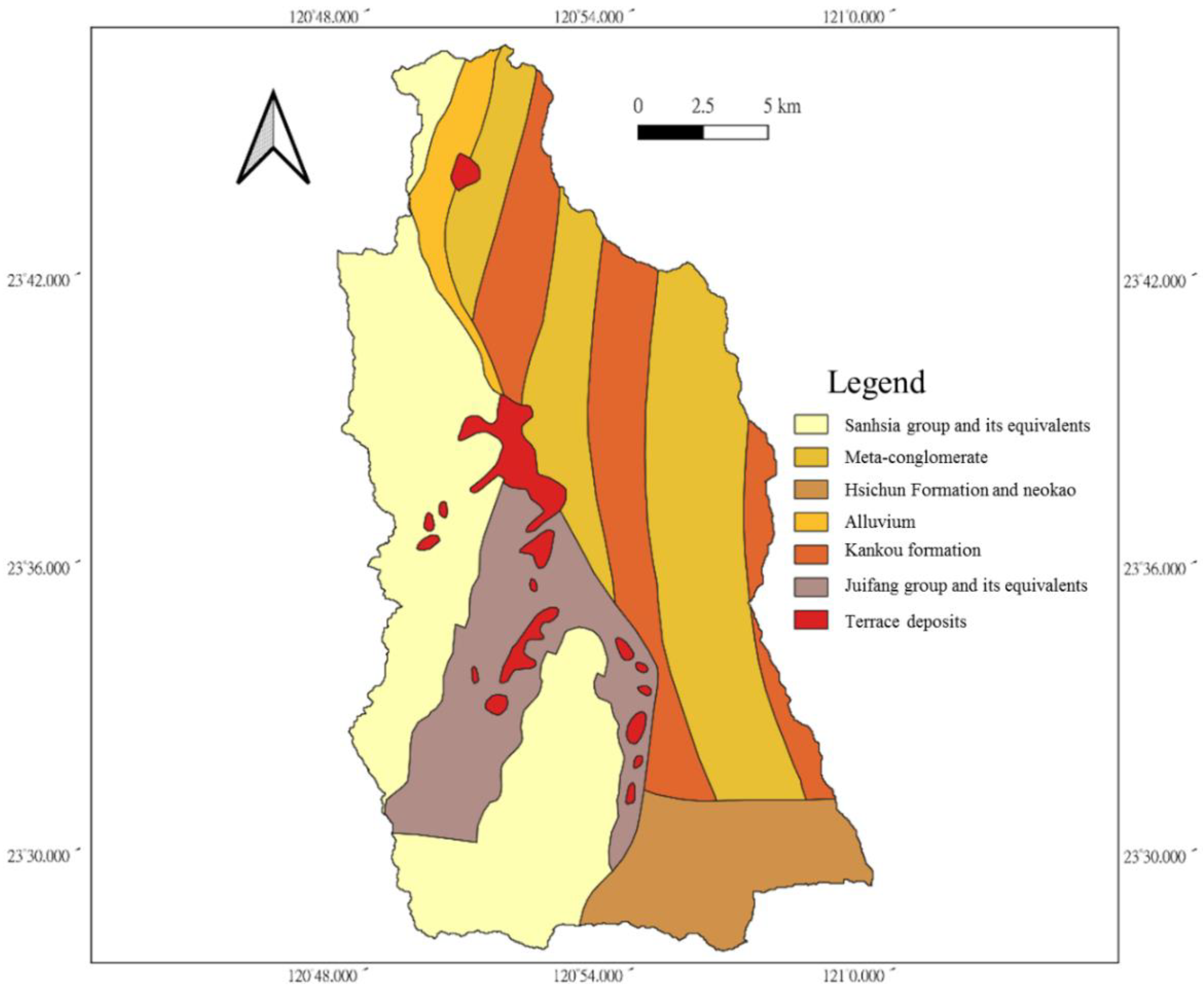
The average elevation in the Chenyoulan watershed is 1588 m, and in only a small part of the area is it less than 500 m. Most of the slopes in the watershed are steeper than 55%. The geology of this area can be roughly divided into two parts, the east and the west, as shown in Figure 2. Most of the west side is composed of sandstone, shale, and sand-shale interbedded sedimentary rocks. The east side comprises mostly metamorphic rocks, mainly slate and quartzite.
2.2. Research-Case Selection
We first examined data held by the Central Meteorological Bureau of the Ministry of Communications on severe weather that affected the Chenyoulan watershed (Table 1) [12]. Our inclusion criteria were rainfall events in which either (1) 40 mm of rain fell within one hour, or (2) 200 mm of rain fell within a 24-h period. The selected data were then compared against Satellite pour l’Observation de la Terre (SPOT) images provided by the National Central University Space and Telemetry Research Center. This process resulted in the identification and selection of six typhoons: Mindulle (2004), Haitang (2005), Kalmaegi (2008), Sinlaku (2008), Morakot (2009) and Saola (2012).
2.3. Satellite Imaging by SPOT
In this study, the Raster Calculator function of QGIS software was used to calculate the normalized-difference vegetation index (NDVI) value of each period of images. Then, the NDVI image-subtraction method was used to find the critical difference in NDVI before and after each weather event. Specifically, the average NDVI before the event was adopted as one of the material factors; the higher this average value, the better the vegetation cover. In the above-mentioned subtraction process, slopes of less than 10 degrees were filtered out, as a straightforward means of excluding most waterways and large buildings. It was then nested within the landslide catalogue described in the next paragraph to find the appropriate NDVI difference.
In this approach, verification methods are divided into three types—landslide group accuracy, non-landslide group accuracy, and overall accuracy—which are computed as follows
2.4. Screening of Terrestrial Factors
2.5. Selection of Material Factors
Our material factors database, which was used to facilitate statistical analysis of the watershed area’s landslide potential, was generated from numerical geological maps. It is divided into three main parts—stratum type, distance from the catchment area to the fault, and average NDVI before the event—and its scoring standard was adopted from Wu and Chen (2005) [18] (see Table 3 and Table 4). Its data-creation methods are described in the three subsections that follow.
2.5.1. Geological Materials: Strata Types
The scale of the numerical geological maps used was 1:250,000. In terms of scores, if the landslide ratio is higher, the formation score is higher, which means that the formation is more fragile. The lower the formation score is, on the other hand, the stronger the formation is. After the data is sorted, it is possible to select data pertaining to specific types of strata in the watershed with high potential for landslides, calculated according to the proportion of each stratum in the watershed area and its weight. Finally, area ratio of catchment can be summarized and counted.
2.5.2. Geological Structure: Distance to Fault
This study’s main type of data on geological structure is distance to the fault that passes through the centroid of the catchment area. These data overlap with the potential watersheds in the Chenyoulan River, and then the catchment area calculates the distance from the fault in each such watershed. Finally, the catchment area distance to fault summarizes the statistics.
2.5.3. Vegetation Status: Pre-Event Average NDVI
The average NDVI value before a given typhoon event in this study was calculated in the first instance for individual SPOT images. Then, the zonal statistics function in QGIS software was used to calculate the average NDVI value for the whole catchment area. The results are summarized in Table 3 and Table 4.
2.6. Inducing Factors
Rainfield cutting is a set of methods used to make sense of rainfall data’s relationship to major rainfall events that cause slope damage, as shown in Table 5 [20]. In this study, Method 5 was adopted for rainfield division. This was because Methods 1, 2 and 4 cut rainfield into time periods too long, which significantly reduces the average intensity value, while Method 3 errs in the opposite direction, making some rainfall data too easy to ignore. Of Methods 5 and 6, the latter has a longer delay time, which also reduces average rainfall intensity.
3. Results and Discussion
Our use of discriminant analysis, logistic regression analysis, and artificial neural network judgment yielded the following conclusions. First, the accuracy rate for a prospective large-scale landslide was 92.2% for logistic analysis and 89% for discriminant analysis. The discriminant analysis (73.7%) and logistic regression analysis (48.1%) had the highest and lowest accuracy rates for predicting large-scale landslides, respectively. The comparable percentages for logit regression and discriminant analysis were 98.4% and 91.1%, respectively, for the overall forecast of no large-scale landslides. The logistic regression model used in discriminant analysis has good AUCs of 0.824 and 0.732, showing that both of these models are suitable for this use, as can be seen from the AUC of the ROC curve. According to the results of our clustering research, large-scale sand and soil disasters are more likely to occur when the catchment region’s total area, total curvature, and average slope are higher.
3.1. Interpretation of Landslides in SPOT Images
This research adopted the landslide-catalogue utilization approach proposed by Hong (2010) [21], and a landslide classification provided by the Central Geological Survey, MOEA [22].
Where A1 refers to land on which landslides have occurred and which is judged accordingly; A2, to land on which landslides have actually occurred but are judged not to have occurred; A3, to land unaffected by landslides but misjudged to have been; and A4, to land that actually is, and is judged to be, unaffected by landslides.
The results of marrying our Typhoon Haitang data with the 2005 landslide catalogue are shown in Table 6, while Table 7 presents the Typhoon Morakot data in combination with the 2009 landslide catalogue.
As can be seen from Table 2 and Table 3, when the NDVI difference is 0.25, fewer parts of the focal area are not covered by debris, so landslide accuracy is quite low. When the NDVI difference is 0.15, such coverage is too large, so the landslide accuracy is high but the overall accuracy is low. The NDVI difference value of 0.2, i.e., halfway between 0.15 and 0.25, was found to be the most consistent of the three. This result, which is regarded as a non-vegetated area, is consistent with the average NDVI before the event minus the post-event NDVI as published by the Agricultural and Forestry Aeronautical Survey Institute of the Forestry Bureau of the Council of Agriculture, Executive Yuan. For the purposes hereof, it is considered to be the landslide itself or an area destroyed by it. After determining the critical difference of NDVI, and ignoring slopes of 10 degrees or less for the reasons mentioned above, we were thus able to ascertain the location of the landslide damage to the Chenyoulan watershed by each typhoon. Then, the total damaged area of the watershed in each case was calculated using QGIS software’s insert function. In cases where this total damaged area was more than 10 hectares in extent, we consider that the total landslide areas of the catchment area is more than 10 hectares as damage. The landslides surface here is not a single block of damage. After confirming the damage area information, the subsequent landslides-related factor analysis can be carried out.
3.2. Statistical Analysis of Terrestrial Factors
After the terrestrial factors were computed, Pearson’s correlation coefficient test was carried out, and the resulting correlation matrix is shown in Table 8. Where the absolute value of the eigenvector is greater than 0.7, it indicates a significant correlation, while 0.3–0.7 is a moderate correlation, and below 0.3, a low one (Pratsins et al., 1988) [23]. Principal component analysis (PCA) was then used to extract the most influential factors in the occurrence of landslide. Ideally, the principal components retained following PCA should explain more than 70% of the overall variance observed.
The Kaiser (1960) criterion holds that it is better to retain those principal-component analyses whose variance is greater than or equal to 1. It can be seen from Table 9 that, beginning with the third principal component, the eigenvalues are all less than 1, which means that the influence of the third and subsequent components on the variables is very weak. Therefore, only the first and second principal components were selected [24].
Table 10 [23] presents the eigenvector results of PCA. From the correlation test results (Table 5), it can be seen that in the first principal component, average elevation of the catchment area, average slope of the catchment area, roughness and TRI are highly correlated, suggesting that this component will be a versatile one for future practical applications. Here, in the first principal component, the most commonly used factor in each study and the average slope of the catchment area with less regional influence is selected. In the second principal component, the correlation between TPI and total curvature was 0.706; the correlation between the two factors was high; and total curvature has also been used widely. Therefore, TPI was deleted. The factors selected for the second principal component were therefore total area of the catchment area and total curvature. Thus, the final influencing factors selected for use in the remainder of this study were total area of the catchment area, average slope of the catchment area, and total curvature.
3.3. Inspection of the Rainfield Cutting Pearson
After rainfield cutting was performed for each of our six typhoons, a rainfall distribution map for each of these events was drawn using the Kriging method, and the Pearson’s correlation coefficients checked again. Table 11 presents the normalized coefficients for five different types of rainfall data. The correlation matrix between these various potential landslide-inducing factors shows that the characteristic values of cumulative rainfall, maximum daily rainfall and maximum 24-h rainfall are all greater than 0.7, indicating that these three inducing factors are highly correlated. Both maximum hourly rainfall and average hourly rainfall are relatively independent, but the latter cannot be known until the end of a rainfall event. Compared with the maximum daily rainfall and accumulated precipitation, maximum daily rainfall is faster and more convenient to obtain. Given that the main purpose of this study is to facilitate rapid early warning of landslides, we deemed it most appropriate to use both the maximum daily rainfall and the maximum hourly rainfall as our key landslide-inducing factors.
Data on terrestrial factors, materials, and causing factors were converted into categorical variables for categorization purposes, with their occurrence classed as “1” and their non-occurrence as “0”. The primary impact data on the potential for landslides included the following eight components in three dimensions: (1) Geological factors, such as the catchment area’s total size, average slope, and total curvature; (2) Material elements, such as the stratum type, proximity to the fault, and pre-event average NDVI; and (3) Inducing factors, such as the catchment area’s maximum daily and hourly rainfall.
3.4. Results of Discriminant Analysis
The coefficients of our discriminant analysis are shown in Table 12, and the coefficient vector of the Fisher discriminant function is calculated as follows:
The Fisher difference function between the occurrence and the non-occurrence of a landslide is computed as
where X1 is total area of the catchment area; X2 is stratum type; X3 is distance from fault; X4 is average slope of the catchment area; X5 is total curvature; X6 is maximum daily rainfall; X7 is average NDVI before the event; and X8 is hourly rainfall.
In the discriminant analysis, if Z is greater than 0, it can be concluded that a landslide has occurred (i.e., the prediction category is “1”). Conversely, if Z is less than 0, a landslide is not deemed to have occurred (prediction category: “0”). The judgment results of the discriminant analysis function are shown in Table 13. Based on Fisher’s discriminant function analysis in multivariate statistical analysis, the interpretation accuracy rates were 89.8% for the training sample, 84.9% for the verification sample, and 89% overall.
3.5. Results of Logistic Regression Analysis
Next, the eight landslide-potential factors were subjected to logistic regression analysis, using the following formula,
in which P is the probability of landslides; L is the landslide factor from Formulas (4) and (5), below; and W is the regression coefficient. The weight coefficients of each factor are shown in Table 14, and the multinomial expressions of logistic regression analysis are as follows:
Then, the result obtained using Formulas (4) and (5) was run through Formulas (3) and (4) to obtain a value, p, for the probability of landslide. If p is greater than or equal to 0.5, landslides is deemed to have occurred, whereas if p is less than 0.5, it is not (see Table 15). The accuracy rate of interpretation of the training sample was 93.7%; of the verification sample, 84.9%; and of the whole dataset, 92.2%. These results are considered poor, insofar as the ratio of occurrence to non-occurrence in logistic regression analysis should be 1:1. This is because large-scale landslide events themselves are relatively few, and the difference in the parental number itself is relatively large.
3.6. Back-Propagation Neural Network Judgment Results
After normalization, the eight selected factors for landslide potential were input into IBM SPSS for analysis and processing.
3.6.1. Normalization
Due to the different ranges of data for each landslide factor, it was necessary to normalize the input parameters before training the neural network, to improve its accuracy and efficiency and prevent convergence difficulties. In this case, normalization was via the mapping method, with the data converted to values ranging between 0.1 and 0.9, as follows,
where a = (Xmax − 9 Xmin)/8; b = (Xmax − Xmin)/0.8; X is the actual value; Xmax is the maximum actual value; and Xmin is the minimum actual value.
Xnorm = (X + a)/b
3.6.2. Back-Propagation Neural Network
The results of our previous analyses of the six focal typhoon events were input into SPSS simultaneously for analysis by a back-propagation neural network, divided into training and validation samples consisting of 70% and 30% of the data, respectively. The results of back-propagation neural network analysis, presented in Table 16, indicate that this technique’s interpretation accuracy rates were 94% for the training sample, 92.9% for the verification sample, and 93.7% overall. The relative importance of each of the eight factors is shown in Table 17.
3.7. Receiver Operating Characteristic Curve
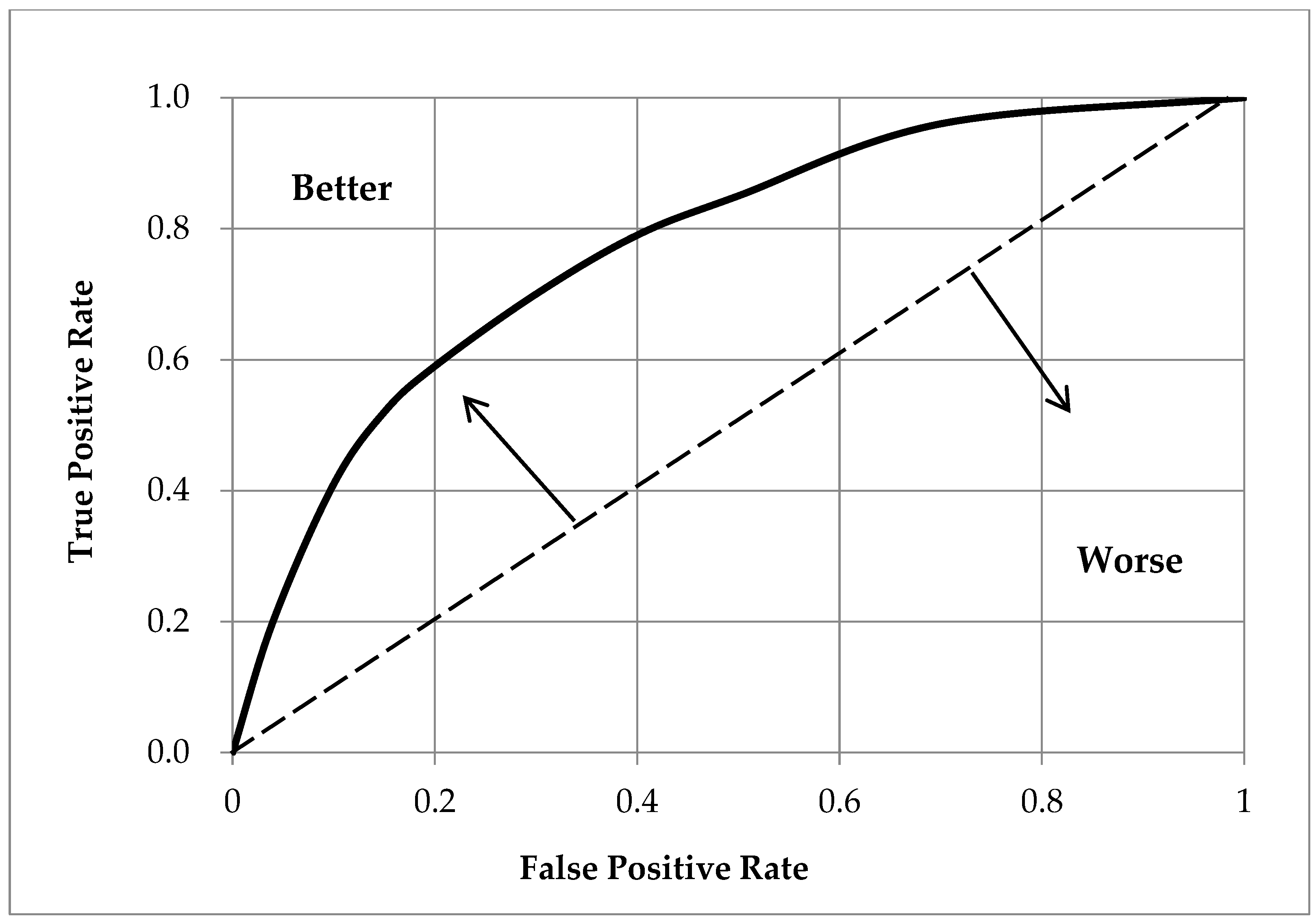
The receiver operating characteristic (ROC) curve is a coordinates-based graphical-analysis tool, consisting of a false positive rate (FPR) as its X axis and a true positive rate (TPR) as its Y axis. FPR can be broadly defined as clarity, and TPR as sensitivity. If the ROC curve is above the diagonal line and curved towards the upper left, it means that the classification result is good, while any other shape indicates that such result is poor (Figure 3).
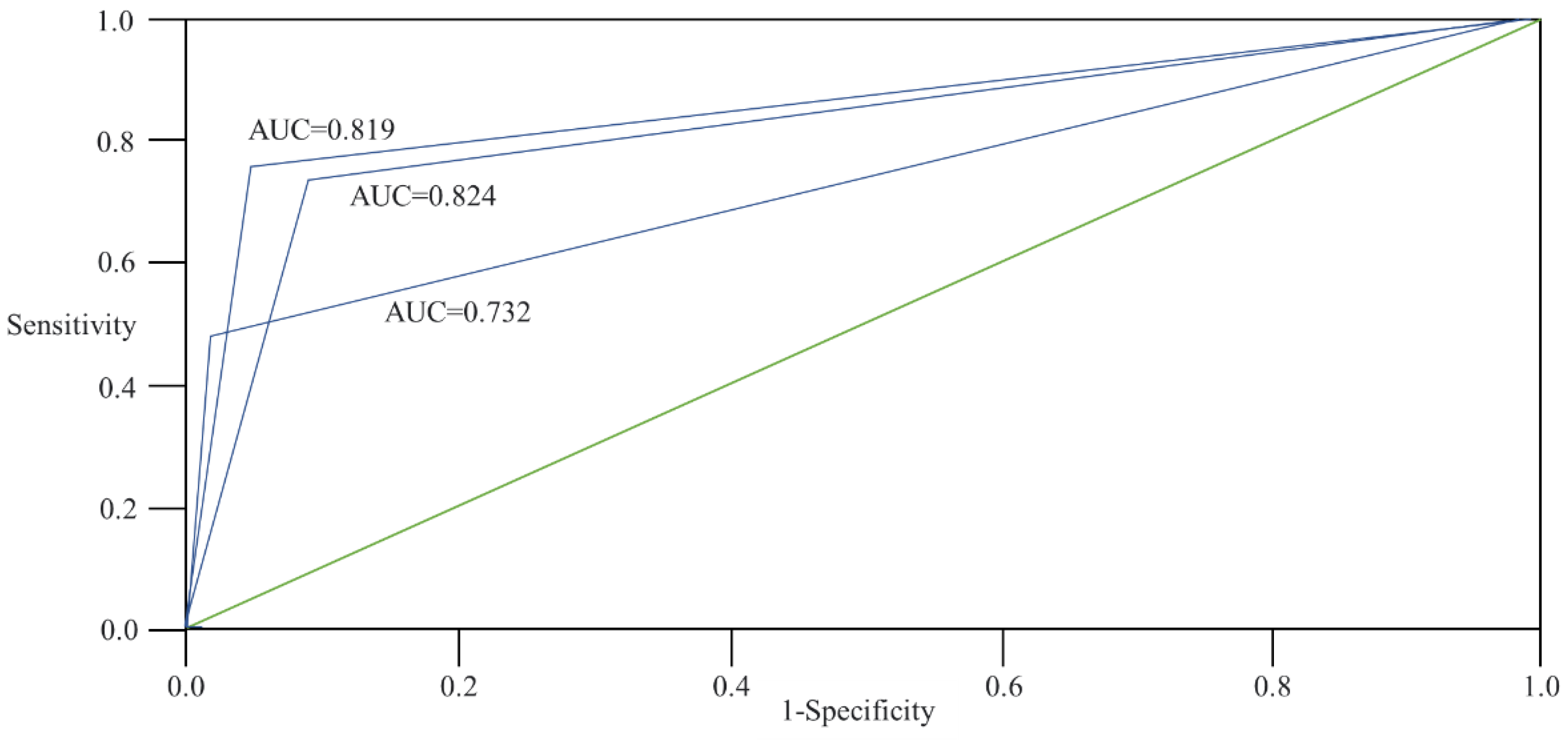
The meanings of various area under curve (AUC) values are shown in Table 18. Specifically, the AUC of discriminant analysis was 0.824, and of logistic regression analysis, 0.732, meaning that both had good discriminative abilities.
Here, the main analysis output is the type of binary classification model, such as occurrence/non-occurrence. When the data-output result is continuous, a threshold value should be set to devide. The formulas for calculating the X axis/FPR and Y axis/TPR are as follows,
with TP and TN being the accuracy and error of the interpretation, respectively, as shown in Table 19. The accuracy of landslide interpretation is mainly discussed in terms of observed value and predicted value. The value of AUC is always between 0 and 1, and the larger the AUC value, the better the accuracy of the interpretation. When the AUC is 1, it means that perfect classification has been achieved (though this seldom happens). AUC values above 0.5 mean that the model has predictive value, and above 0.7, that such prediction is accurate. When AUC is exactly 0.5, it is a random guess in the table; and when it is less than 0.5, it means that the model has no use value (Table 16).
The ROC curves of each of this paper’s modes of analysis are shown in Figure 4. From the AUC of the ROC curve, it can be seen that for large-scale landslides, the neural-network AUC was 0.819; the discriminant-analysis AUC, 0.824; and the logistic-regression AUC, 0.732, indicating that the results of the three models could be used.
3.8. Comparison of Three Analysis Modes
The present study of three potential means of analyzing and predicting large-scale landslides found, firstly, that a artificial neural network is relatively complex and cannot be applied in the form of formulas, whereas the other two models are relatively simple, and can be. Second, when it came to potential large-scale landslide, the artificial neural network accuracy rate was the highest, at 93.7%, and discriminant analysis the lowest, at 89%. Third, in overall large-scale landslide prediction, the accuracy rate of discriminant analysis was the highest, at 73.7%, and lowest for logistic regression, at 48.1%. Fourth, in predicting that no large-scale landslide would occur, logistic regression performed best, at 98.4%, and discriminant analysis the worst, at 91.1%. And fifth, the best AUC of the ROC curve was discriminant analysis, at 0.824, and the worst, logistic regression, at 0.732. In short, all three models were found to have distinct advantages and disadvantages for this purpose. The reason for the less-accurate prediction of landslides than of their non-occurrence may have been that the number of the former events was far smaller than that of the latter.
3.9. Results of Cluster Analysis of Catchment Areas’ Landslide Potential
A total of 219 probably landslide-prone areas within the Chenyoulan River watershed were classified according to the factors named above. Among them, the five fixed ones—i.e., total area of the catchment, average slope of the catchment, total curvature, type of stratum, and distance from the fault—were used as the variables for cluster analysis. The number of clusters was determined by Ward’s method of hierarchical analysis, and then K-means clustering was applied.
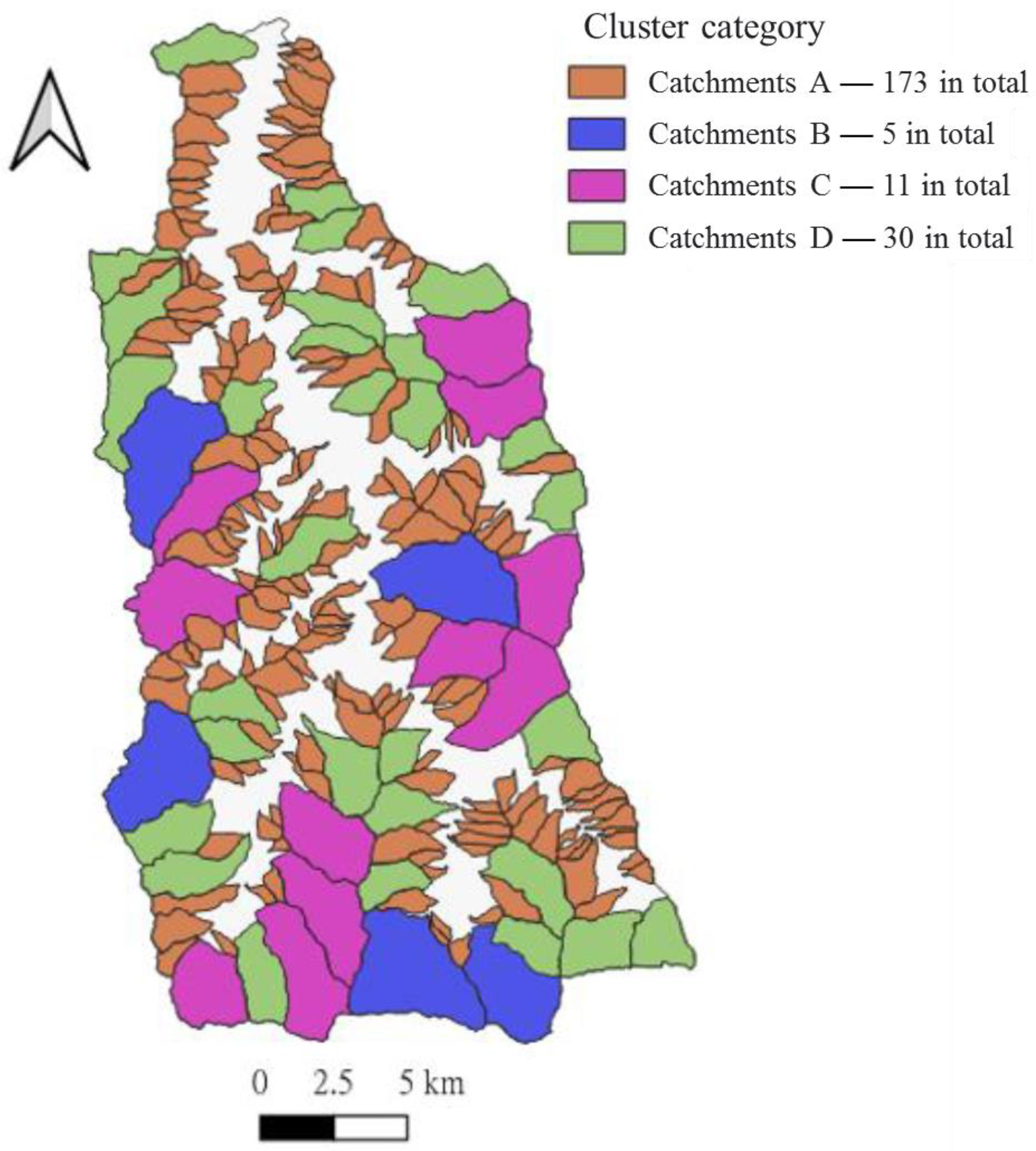
First, Ward’s method established that the catchment area could be roughly divided into four types of clusters according to the characteristics of its factors. For a single cluster, the smaller the spatial distance between the data, the earlier they will be merged; and the earlier a catchment area is merged, the more similar its factor characteristics are to feature. The classification results are shown in Table 20, and the distribution positions in Figure 5.
3.9.1. Cluster A: Small Catchment Areas
Cluster A comprises the 173 catchment areas that are the smallest in extent, and have moderate stratigraphic conditions, the shortest distances to the fault, the least steep average slopes, and the smallest total curvature.
3.9.2. Cluster B: Large Catchment Areas
The five catchments making up cluster B have the largest area, good stratigraphic conditions, long distances to the fault, steep slopes and large total curvature.
3.9.3. Cluster C: Fragile Strata Catchment Areas
The 11 catchments in the C cluster are second in extent only to those of the B cluster. Their stratigraphic conditions are poor, their distance to the fault the farthest, their slopes steep, and their total curvature large.
3.9.4. Cluster D: Curvature Small Catchment Area
In the D cluster, the 30 catchments’ surface areas are the second smallest. Their stratigraphic conditions are moderate; their distance to the fault, relatively short; their slopes, gentle; and their total curvature, the smallest.
3.9.5. Discuss of Cluster Analysis of Catchment Areas’ Landslide Potential
Key statistics about the current study’s six focal typhoons are shown in Table 21. Across all six of these weather events, the proportions of all major landslides by affected cluster type were: D, 40%; A, 26.3%; C, 21.3%; and B, 12.5%. The landslide-struck areas of each cluster as a proportion of all areas in that cluster, on the other hand, were: B, 66.7%; C, 51.5%; D, 35.6%; and A, 4.1%. From this, it can be seen that the likelihood of landslides affecting Clusters B and C is relatively high; but because Cluster A accounts for the majority of sites in the focal region, damage to Clusters B and C will be masked in the total damage ratio.
From Table 22, it can be seen that in each typhoon event, the rate of occurrence of landslides was the highest for Cluster B and lowest for Cluster A. Table 23, meanwhile, shows maximum daily rainfall and maximum hourly rainfall on a typhoon-by-typhoon basis, and relates this information to the total number of damaged areas in the region.
It can be seen from the above that the total catchment area, total curvature, and average slope of clusters B and C are larger than those of clusters A and D. The damage incidence rates of clusters B and C are also greater than those of the other two clusters. Therefore, it is reasonable to suppose that large-scale debris-flow disasters are more likely to occur if—among its fixed characteristics—the total area, total curvature, and average slope of the catchment area are larger.
The results of neural-network analysis and cluster analysis differ, as shown in Table 17. This is likely rooted in the fact that the purpose of the former is to build a model, whereas the latter merely divides items into groups according to their factor characteristics.
The physical determination approach is primarily employed in regions with few landslides and there is little quantitative study on the relationship between rainfall and landslide stability, but it does have some disaster preventive effects on the stability evaluation of rainfall-induced landslides. The likelihood of a large-scale landslide brought on by rain is examined in this study, however there are numerous other components and evaluation techniques. According to Wang et al., (2020), integrating a hydrological model with a 1 km resolution with a slope stability model with a 90 m resolution results in landslide prediction with a worldwide accuracy and true positive rate of 97.2% and 66.9%, respectively [26]. A more precise estimation of shallow landslide susceptibility due to a region’s typical rainfall triggering pattern was made possible by Bordoni et al., (2020) in their study, Shallow landslides susceptibility obtained from a multitemporal inventory, which grouped landslides that occurred in more events over several years [27]. He et al., (2021) used that 3D models to predict landslides, and their proposed rainfall threshold analysis can serve as a guide for the times when the majority of landslides typically occur in the absence of appropriate data. It also serves as a crucial indicator for disaster early warning and prediction [28]. All methods for assessing large-scale landslides have excellent early warning capabilities. A suitable early warning system for disasters is chosen to lessen their likelihood and impact based on their features and those of the surrounding environment.
4. Conclusions
This study looked at the potential for large-scale landslides to damage 219 parts of the watershed along Taiwan’s Chenyulan River. Eight components were selected after principal component analysis and correlation analysis were used to evaluate the impact variables for such events. According to statistical analysis of these factors, the average maximum daily rainfall associated with large-scale landslides over the course of six different typhoon strikes on the watershed in question was 459 mm, while the average maximum daily rainfall associated with no large-scale landslides was 395 mm. The main objective of this work is to examine potential large-scale landslides in relation to landslide and rainfall influence elements. Discriminant analysis and artificial neural networks, which have a favorable warning impact for areas that grow after disasters, have an accuracy rate of about 70% when it comes to predicting large-scale landslides, according to the research findings. When used to forecast non-large-scale landslides, all three approaches had an accuracy rate of more than 90%, with neural networks and logistic regression analysis having the greatest accuracy rates at more than 97–98%. To prevent large-scale landslide catastrophes, decrease the impact of disasters, and assure the protection of people and property, disaster planners can build warning zones. The information from this study is useful for both disaster preparedness and early detection of major landslide events. Limitations of this study Since the gunshot frequency has an impact on SPOT satellite imaging, the debris flow that happened during the early rainstorm event cannot be completely excluded from the event.
Author Contributions
Conceptualization, J.-Y.L.; data curation, C.-L.W.; writing—original draft, C.-L.W.; writing—original draft, writing—review and editing, J.-C.C.; supervision, J.-Y.L. All authors have read and agreed to the published version of the manuscript.
Funding
This research received no external funding.
Institutional Review Board Statement
Not applicable.
Informed Consent Statement
The authors declare no conflict of interest.
Data Availability Statement
The data presented in this study are available in the article.
Conflicts of Interest
The authors declare no conflict of interest.
References
- Large-Scale Landslide, Soil and Water Conservation Bureau, COA. Available online: https://246.swcb.gov.tw/Landslide/ (accessed on 18 July 2022).
- Varnes, D.J. Slope Movement Types and Processes. In Special Report 176: Landslides: Analysis and Control; Schuster, R.L., Krizek, R.J., Eds.; Transportation and Road Research Board, National Academy of Science: Washington, WA, USA, 1978; pp. 11–33. [Google Scholar]
- Santacana, N.; Baeza, B.; Corominas, J.; Paz, A.D.; Marturiá, A. GIS-Based Multivariate Statistical Analysis for Shallow Landslide Susceptibility Mapping in La Pobla de Lillet Area (Eastern Pyrenees, Spain). Nat. Hazards 2020, 30, 281–295. [Google Scholar] [CrossRef]
- Liu, J.K.; Shih, T.Y. Collection and application of 3D space information with airborne lidar technology. J. Civ. Hydraul. Eng. 2009, 36, 52–63. [Google Scholar]
- Renwick, W.; Brumbaugh, R.; Loeher, L. Landslide Morphology and Processes on Santa cruz Island, California. Geogr. Annaler. Ser. A Phys. Geogr. 1982, 64, 149–159. [Google Scholar] [CrossRef]
- Fell, R.F.; Hungr, O.; Leroueil, S.; Riemer, W. Keynote Lecture—Geotechnical Engineering of The Stability Of Natural Slopes, And Cuts And Fills In Soil. In Proceedings of the International Conference on Geotechnical and Geological Engineering, Melbourne, Australia, 19–24 November 2000; Technomic Publishing Co.: Lancaster, PA, USA, 2000. Available online: https://www.researchgate.net/publication/267403410_Keynote_lecture-Geotechnical_engineering_of_the_stability_of_natural_slopes_and_cuts_and_fills_in_soil (accessed on 9 November 2022).
- Giannecchini, R. Relationship between rainfall and shallow landslides in the southern Apuan Alps (Italy). Nat. Hazards Earth System Sci. 2006, 6, 357–364. [Google Scholar] [CrossRef]
- No. 4115; Public Works Research Institute Sediment Management Research Group Volcano/Debris Flow Team: Public Works Research Institute Material. PWRI: Tsukuba, Japan, 2008.
- Minami, N. Deep-seated Landslide and administrative measures, International Symposium on Slopeland Disaster Mitigation, SWCB et al., Taichung, Taiwan. 2010 International Landslide Disaster Technology Exchange Conference.
- Chigira, M. September 2005 rain- induced catastrophic rockslides on slopes affected by deep-seated gravitational deformations, Kyushu, southern Japan. Eng. Geol. 2009, 108, 1–15. [Google Scholar] [CrossRef]
- Taiwan-Large-Scale Landslides, National Science and Technology Center for Disaster Reduction. Available online: https://tccip.ncdr.nat.gov.tw/ark_02_case_one.aspx?case_id=LS02 (accessed on 18 July 2022).
- Rainfall Classification by the Central Meteorological Bureau of the Ministry of Communications. 2020. Available online: https://www.cwb.gov.tw/V8/C/K/CommonFaq/rain_all.html (accessed on 15 July 2020).
- Huang, H.J. Talking about the landslide of the Forest. Taiwan For. J. 2008, 12, 54–64. [Google Scholar]
- Lin, C.R. A Study on the Application of Potential Hazard Index to the Watershed Classification and Regionalization at Pingtung. Master’s Thesis, Department of Soil and Water Conservation, National Pintung University of Science and Technology, Pingtung, Taiwan, 2004. [Google Scholar]
- Wang, L.J.; Guo, M.; Sawada, K.; Lin, J.; Zhang, J. Landslide susceptibility mapping in Mizunami City, Japan: A comparison between logistic regression, bivariate statistical analysis and multivariate adaptive regression spline models. Catena 2015, 135, 271–282. [Google Scholar] [CrossRef]
- Shou, K.J. Study on the Control Factors of Rainfall Induced Landslides in Central Taiwan. Master’s Thesis, Department of Civil Engineering, National Chung Hsing University, Taichung, Taiwan, 2007. [Google Scholar]
- Wu, B.Y. Landslides and Engineered Slopes. In The Past to the Future, Two Volumes + CD-ROM; Chapter: Analysis of control factors for landslides in Central Taiwan area; CRC Press: Boca Raton, FL, USA, 2006. [Google Scholar]
- Chen, H.H. Application of Satellite Imagery for Nan-Chin Road Potential Landsliding Analysis. Master’s Thesis, Department of Environmental Engineering and Science, Feng Chia University, Taichung, Taiwan, 2005. [Google Scholar]
- Wu, C.H.; Chen, S.C. A Landslide Potential Model for Ming-De Reservoir Watershed. J. Soil Water Conserv. 2005, 37, 155–168. [Google Scholar]
- Jan, C.D. Rainfall Threshold Criterion for Debris-Flow Initiation, Soil and Water Conservation Bureau. Master’s Thesis, National Cheng Kung University, Tainan, Taiwan, 2002. [Google Scholar]
- Hong, C.Y. Time Series Analysis of Control Factors of Landslides in Central Taiwan. Master’s Thesis, Department of Civil Engineering, National Chung Hsing University, Taichung, Taiwan, 2010. [Google Scholar]
- Landslide Classification by Central Geological Survey, MOEA. Available online: https://www.moeacgs.gov.tw/eng/Faqs/faqs (accessed on 8 July 2020).
- Pratsinis, S.E.; Zeldin, M.D.; Ellis, E.C. Source Resolution of the Fine Carbonaceous Aerosol by Principal Componet-Stepwise Regression Analysis. Environ. Sci. Technol. 1988, 22, 212–216. [Google Scholar] [CrossRef] [PubMed]
- Kaiser, H.F. The Application of Electronic Computers to Factor Analysis. Educ. Psychol. Meas. 1960, 20, 141–151. [Google Scholar] [CrossRef]
- Hanley, J.A.; McNeil, B.J. The meaning and use of the area under a receiver operating characteristic (ROC) curve. Radiology 1982, 143, 29–36. [Google Scholar] [CrossRef] [PubMed] [Green Version]
- Wang, S.; Zhang, K.; Beek, L.P.H.; Tain, X.; Bogaard, T.S. Physically-based landslide prediction over a large region: Scaling low-resolution hydrological model results for high-resolution slope stability assessment. Environ. Model. Softw. 2020, 124, 104607. [Google Scholar] [CrossRef]
- Bordoni, M.; Galanti, Y.; Bartelletti, C.; Persichillo, M.G.; Barsanti, M.; Giannecchini, R.; Avanzi, G.D.; Cevasco, A.; Brandolini, P.; Galve, J.P.; et al. The influence of the inventory on the determination of the rainfall-induced shallow landslides susceptibility using generalized additive models. CATENA 2020, 193, 104630. [Google Scholar] [CrossRef]
- He, J.Y.; Qiu, H.J.; Qu, F.H.; Hu, S.; Yang, D.D.; Shen, D.D.; Zhang, Y.; Sun, H.S.; Cao, M.M. Prediction of spatiotemporal stability and rainfall threshold of shallow landslides using the TRIGRS and Scoops3D models. CATENA 2021, 197, 104999. [Google Scholar] [CrossRef]
Figure 1.
Location map of the Chenyoulan watershed.

Figure 2.
Stratigraphic distribution map of the Chenyoulan watershed.

Figure 3.
Schematic of a receiver operating characteristic curve as indicative of classification accuracy.
Figure 3.
Schematic of a receiver operating characteristic curve as indicative of classification accuracy.

Figure 4.
Receiver operating characteristic curve, discriminant analysis, logistic regression analysis, and artificial neural network; AUC = area under curve.
Figure 4.
Receiver operating characteristic curve, discriminant analysis, logistic regression analysis, and artificial neural network; AUC = area under curve.

Figure 5.
Distribution of clusters.


Table 1.
Rainfall classification by the Central Meteorological Bureau of the Ministry of Communications.
Table 1.
Rainfall classification by the Central Meteorological Bureau of the Ministry of Communications.
| Type of Alert | Rainfall Classification | Definition |
|---|---|---|
| Heavy rain special | Heavy rain | Above 80 mm/24 h or 40 mm/1 h |
| Torrential rain | Extremely heavy rain | Above 200 mm/24 h or 100 mm/3 h |
| Torrential rain | Above 350 mm/24 h or 200 mm/3 h | |
| Extremely torrential rain | Above 500 mm/24 h |
Table 2.
Terrestrial factors.
| Parameter | Description of Calculation | Meaning (Where Not Self-Explanatory) |
|---|---|---|
| Total area of catchment | A = a × n A: grid area [];n: number of grids | |
| Average elevation of catchment area | {h: elevation of the grid} | |
| Average slope of catchment area | {slope: slope value of the grid} | |
| Total curvature | {Z: total curvature of the grid} | The rate of change representing the slope or direction of slope |
| Roughness | The difference between the maximum and minimum of the surrounding elevation | |
| Terrain Ruggedness Index, TPI | The center-point elevation minus the average of the surrounding elevations | |
| Topographic Position Index, TRI | The average of the difference between the elevation of the center point and the surrounding elevation |
Table 3.
Strata scoring criteria.
| Formation Name | Score | Landslide Ratio | Formation Name | Score | Landslide Ratio |
|---|---|---|---|---|---|
| Sanhsia group and its equivalents | 10 | 2.8% | Tatungshan formation | 1.91 | 0.28% |
| Meta-conglomerate | 9.76 | 2.73% | Terrace deposits | 1.87 | 0.27% |
| Lushan formation | 7.42 | 2% | Toukoshan formation and its equivalents | 1.8 | 0.25% |
| Chinshui shale and its equivalents | 6.73 | 1.78% | Cholan formation and its equivalents | 1.79 | 0.25% |
| Kankou formation | 5.81 | 1.5% | Hsichun formation and Neokao formation | 1.28 | 0.09% |
| Juifang group and its equivalents | 3.81 | 0.87% | Alluvium | 1.03 | 0.01% |
| Yehliu group and its equivalents | 3.69 | 0.84% | Lateritic terrace deposits | 1.03 | 0.01% |
| Tananao schists | 2.21 | 0.38% | Basic rock | 1 | 0% |
Note. Source: Wu and Chen (2005) [19].
Table 4.
Scoring criteria for fault assessment.
| Distance between Assessment Point and Fault Zone | Score | Distance between Assessment Point and Fault Zone | Score |
|---|---|---|---|
| <100 m | 10 | 600–700 m | 4 |
| 100–200 m | 9 | 700–800 m | 3 |
| 200–300 m | 8 | 800–900 m | 2 |
| 300–400 m | 7 | 900–1000 m | 1 |
| 400–500 m | 6 | >1000 m | 0 |
| 500–600 m | 5 |
Note. Source: Wu and Chen (2005) [19].
Table 5.
Six rainfield-cutting methods.
| Method | Correction Method | Start of Rain | End of Rain | Method |
|---|---|---|---|---|
| 1 | No rain for previous 24 h | No rain for 24 consecutive hours | 1 | |
| 2 | 1 | No rain for previous 12 h | No rain for 12 consecutive hours | 2 |
| 3 | Hourly rainfall is greater than 4 mm | Rainfall is less than 4 mm for three consecutive hours | 3 | |
| 4 | Cumulative rainfall is at least 10 mm in the first 24 h | Cumulative rainfall is less than 10 mm for 24 h | 4 | |
| 5 | 3 | Hourly rainfall is greater than 4 mm | Rainfall is less than 4 mm for six consecutive hours | 5 |
| 6 | 4 | Cumulative rainfall is at least 10 mm in the first 12 h | Cumulative rainfall is less than 10 mm for 12 h | 6 |
Table 6.
Overlapping results, Typhoon Haitang and the 2005 Landslide Catalogue.
| Accuracy NDVI Difference | Landslide Accuracy | Non-Landslide Accuracy | Overall Accuracy |
|---|---|---|---|
| 0.15 | 83.6% | 86.9% | 86.6% |
| 0.2 | 70.6% | 94.2% | 93.7% |
| 0.25 | 57.4% | 97.2% | 96.3% |
Table 7.
Overlapping results, Typhoon Morakot and the 2009 Landslide Catalogue.
| Accuracy NDVI Difference | Landslide Accuracy | Non-Landslide Accuracy | Overall Accuracy |
|---|---|---|---|
| 0.15 | 72.7% | 86.6% | 86.3% |
| 0.2 | 61.5% | 95.3% | 95.2% |
| 0.25 | 32.6% | 95.5% | 95.5% |
Table 8.
Pearson’s correlation coefficients.
| Total Area of Catchment | Average Elevation of Catchment Area | Average Slope of Catchment Area | Total Curvature | Roughness | TPI | TRI | |
|---|---|---|---|---|---|---|---|
| Total area of catchment | 1.000 | 0.438 | 0.251 | 0.103 | 0.258 | −0.002 | 0.252 |
| Average elevation of catchment area | 0.438 | 1.000 | 0.774 | 0.079 | 0.678 | −0.109 | 0.680 |
| Average slope of catchment area | 0.251 | 0.774 | 1.000 | 0.109 | 0.985 | −0.105 | 0.988 |
| Total curvature | 0.103 | 0.079 | 0.109 | 1.000 | 0.122 | 0.706 | 0.107 |
| Roughness | 0.258 | 0.678 | 0.985 | 0.122 | 1.000 | −0.120 | 0.998 |
| Topo-graphic Position Index, TPI | −0.002 | −0.109 | −0.105 | 0.706 | −0.120 | 1.000 | −0.140 |
| Terrain Rugged-ness Index, TRI | 0.252 | 0.680 | 0.988 | 0.107 | 0.998 | −0.140 | 1.000 |
Table 9.
Total variation interpretation, principal component analysis.
| Ingredient | Initial Eigenvalues | Sum of Squares Loading Extraction | ||||
|---|---|---|---|---|---|---|
| Sum | Variation (%) | Accumulation (%) | Sum | Variation (%) | Accumulation (%) | |
| 1 | 3.686 | 52.661 | 52.661 | 3.686 | 52.661 | 52.661 |
| 2 | 1.614 | 23.055 | 75.716 | 1.614 | 23.055 | 75.716 |
| 3 | 0.951 | 13.587 | 89.303 | |||
| 4 | 0.372 | 5.312 | 94.614 | |||
| 5 | 0.359 | 5.126 | 99.740 | |||
| 6 | 0.016 | 0.233 | 99.973 | |||
| 7 | 0.002 | 0.027 | 100.000 | |||
Table 10.
Characteristic vector table of local factors, principal component analysis.
| Terrestrial Factor | Ingredients | |
|---|---|---|
| One | Two | |
| Total area of catchment | 0.412 | 0.725 |
| Average elevation of catchment area | 0.810 | −0.004 |
| Average slope of catchment area | 0.967 | −0.008 |
| Total curvature | 0.131 | 0.894 |
| Roughness | 0.972 | −0.009 |
| Topographic Position Index, TPI | −0.135 | 0.893 |
| Terrain Ruggedness Index, TRI | 0.972 | −0.029 |
Table 11.
Pearson’s correlation coefficient table.
| Factor | Maximum Daily Rain | Maximum Hourly Rainfall | Mean Hourly Rainfall | Maximum 24-h Rainfall | Cumulative Rainfall |
|---|---|---|---|---|---|
| Maximum daily rain | 1.000 | 0.287 | 0.425 | 0.905 | 0.726 |
| Maximum hourly rainfall | 0.287 | 1.000 | 0.589 | 0.301 | 0.239 |
| Mean hourly rainfall | 0.425 | 0.589 | 1.000 | 0.367 | 0.017 |
| Maximum 24-h rainfall | 0.905 | 0.301 | 0.367 | 1.000 | 0.830 |
| Cumulative rainfall | 0.726 | 0.239 | 0.017 | 0.830 | 1.000 |
Table 12.
Coefficients of Fisher’s discriminant classification function.
| Factor | 0 | 1 | Coefficient Vector (1–0) |
|---|---|---|---|
| Total area of catchment area | −0.001 | 0.010 | 0.01 |
| Type of stratum | 0.895 | 0.865 | −0.03 |
| Distance from fault | 0.857 | 0.855 | −0.002 |
| Average slope of catchment area | 0.770 | 0.775 | 0.005 |
| Total curvature | −14.663 | −15.045 | −0.382 |
| Maximum daily rainfall | 0.024 | 0.031 | 0.008 |
| Average NDVI before the event | 31.857 | 36.255 | 4.397 |
| Hourly rainfall | 0.219 | 0.160 | −0.059 |
| Constant | −33.138 | −38.222 | −5.084 |
Table 13.
Discriminant-analysis judgments.
| Classification Result | Total | |||
|---|---|---|---|---|
| Category | 0 | 1 | ||
| Training sample (1095 rows) | 0 | 891 (91.5%) | 83 (8.5%) | 974 (100%) |
| 1 | 29 (24%) | 92 (76%) | 121 (100%) | |
| Correct discrimination rate = [(891 + 92)/(974 + 121)] × 100% = 89.8% | ||||
| Classification result | Total | |||
| Category | 0 | 1 | ||
| Validation sample (219 rows) | 0 | 160 (88.9%) | 20 (11.1%) | 180 (100%) |
| 1 | 13 (33.3%) | 26 (66.7%) | 39 (100%) | |
| Correct discrimination rate = [(160 + 26)/(180 + 39)] × 100% = 84.9% | ||||
| Classification result | Total | |||
| Category | 0 | 1 | ||
| Overall sample (1314 rows) | 0 | 1051 (91.1%) | 103 (8.9%) | 1154 (100%) |
| 1 | 42 (26.3%) | 118 (73.7%) | 160 (100%) | |
| Correct discrimination rate = [(1051 + 118)/(1154 + 160)] × 100% = 89% | ||||
Table 14.
Table of coefficients for logistic regression.
| Code | Factor | Coefficient | Coefficient Value |
|---|---|---|---|
| Total area of the catchment area | 0.007 | ||
| Type of stratum | −0.045 | ||
| Distance from the fault | 0.018 | ||
| Average slope of the catchment area | 0.043 | ||
| Maximum daily rainfall | 0.008 | ||
| Average NDVI before the event | 3.160 | ||
| Total curvature | −2.639 | ||
| Hourly rainfall | −0.116 | ||
| Constant | −4.473 |
Table 15.
Logistic-regression judgments.
| Classification Result | Total | |||
|---|---|---|---|---|
| Category | 0 | 1 | ||
| Training sample (1095 rows) | 0 | 962 (98.8%) | 12 (1.2%) | 974 (100%) |
| 1 | 57 (47.1%) | 64 (52.9%) | 121 (100%) | |
| Accurate discrimination rate = [(962 + 64)/(974 + 121)] × 100% = 93.7% | ||||
| Validation sample (219 rows) | 0 | 173 (96.1%) | 7 (3.9%) | 180 (100%) |
| 1 | 26 (66.7%) | 13 (33.3%) | 39 (100%) | |
| Accurate discrimination rate = [(173 + 13)/(180 + 39)] × 100% = 84.9% | ||||
| Overall sample (1314 rows) | 0 | 1135 (98.4%) | 19 (1.6%) | 1154 (100%) |
| 1 | 83 (51.9%) | 77 (48.1%) | 160 (100%) | |
| Accurate discrimination rate = [(1135 + 77)/(1154 + 160)] × 100% = 92.2% | ||||
Table 16.
Back-propagation neural network judgments.
| Training Sample (920 Rows) | Classification Result | Total | |||
|---|---|---|---|---|---|
| Category | 0 | 1 | |||
| Original category | Number (920 rows) | 0 | 793 (97.5%) | 20 (2.5%) | 813 (100%) |
| 1 | 35 (32.7%) | 72 (67.3%) | 107 (100%) | ||
| Accurate discrimination rate = [(962 + 64)/(974 + 121)] × 100% = 93.7% | |||||
| Original category | Number (394 rows) | 0 | 327 (95.9%) | 14 (4.1%) | 341 (100%) |
| 1 | 14 (26.4%) | 39 (73.6%) | 53 (100%) | ||
| Accurate discrimination rate = [(173 + 13)/(180 + 39)] × 100% = 84.9% | |||||
| Original category | Number (1314 rows) | 0 | 1120 (97.1%) | 34 (2.9%) | 1154 (100%) |
| 1 | 49 (30.6%) | 111 (69.4%) | 160 (100%) | ||
| Accurate discrimination rate = [(1120 + 111)/(1154 + 160)] × 100% = 93.7% | |||||
Table 17.
Table of coefficients for logistic regression.
| Factor | Significance | Importance of Normalization |
|---|---|---|
| Total area of the catchment area | 0.247 | 100.0% |
| Maximum daily rainfall | 0.206 | 83.2% |
| Maximum hourly rainfall | 0.164 | 66.5% |
| Maximum hourly rainfall | 0.134 | 54.3% |
| Total curvature | 0.077 | 31.3% |
| Type of stratum | 0.065 | 26.3% |
| Average slope of the catchment area | 0.061 | 24.8% |
| Distance from the fault | 0.045 | 18.2% |
Table 18.
Area under curve discrimination-ability thresholds (Hanley and McNeil, 1982) [25].
Table 18.
Area under curve discrimination-ability thresholds (Hanley and McNeil, 1982) [25].
| Value of Area under the Receiver Operating Characteristic Curve (AUC) | Discrimination Ability |
|---|---|
| AUC ≧ 0.9 | Excellent discrimination ability |
| 0.7 ≦ AUC < 0.9 | Good discrimination ability |
| 0.5 ≦ AUC < 0.7 | Fair discrimination ability |
| AUC = 0.5 | No ability to discriminate |
Table 19.
Receiver operating characteristic curve evaluation table.
| Observed Value Predictive Value | Unstable | Stable |
|---|---|---|
| Unstable | TP | FP |
| true positive | false positive | |
| Stable | FN | TN |
| false negative | true negative |
Table 20.
K-means test for group differences.
| Impact Factor | Cluster A | Cluster B | Cluster C | Cluster D | Sort by Size |
|---|---|---|---|---|---|
| Total catchment area (hectares) | 70.152 | 1067.59 | 680.815 | 329.178 | B > C > D > A |
| Type of stratum | 7.444 | 6.220 | 8.902 | 7.395 | C > A > D > B |
| Distance from fault | 2.249 | 0.800 | 0.091 | 1.433 | A > D > B > C |
| Average slope of catchment area (degrees) | 33.086 | 38.294 | 36.486 | 35.002 | B > C > D > A |
| Total curvature (degrees) | −0.0001 | 0.006 | 0.002 | −0.003 | B > C > A > D |
Table 21.
Statistics relevant to the destruction ratio of each cluster.
| Items | Total Number | Number of Destructive Events | Destruction as a Percentage of the Cluster | Percentage of Total Damage |
|---|---|---|---|---|
| Cluster | ||||
| Cluster A | 1038 | 42 | 4.1% | 26.3% |
| Cluster B | 30 | 20 | 66.7% | 12.5% |
| Cluster C | 66 | 34 | 51.5% | 21.3% |
| Cluster D | 180 | 64 | 35.6% | 40% |
Table 22.
Number and percentage of damaged areas per cluster, by typhoon event.
| Cluster | A | B | C | D |
|---|---|---|---|---|
| Typhoon | (173 Areas) | (5 Areas) | (11 Areas) | (30 Areas) |
| Typhoon Mindulle | 0 (0%) | 0 (0%) | 0 (0%) | 0 (0%) |
| Typhoon Haitang | 18 (10.4%) | 5 (100%) | 11 (100%) | 26 (86.7%) |
| Typhoon Kalmaegi | 0 (0%) | 0 (0%) | 0 (0%) | 0 (0%) |
| Typhoon Sinlaku | 4 (2.3%) | 5 (100%) | 7 (63.6%) | 11 (36.7%) |
| Typhoon Morakot | 8 (4.6%) | 5 (100%) | 8 (72.7%) | 13 (43.3%) |
| Typhoon Saola | 12 (6.9%) | 5 (100%) | 8 (72.7%) | 14 (46.7%) |
Table 23.
Number of damaged areas and maximum hourly and daily rainfall, by typhoon event.
| Statistic | Number of Damaged Areas | Maximum Hourly Rainfall (mm/h) | Maximum Daily Rainfall (mm/day) |
|---|---|---|---|
| Typhoon | |||
| Typhoon Mindulle | 0 | 48.4 | 281.6 |
| Typhoon Haitang | 60 | 18.0 | 171.5 |
| Typhoon Kalmaegi | 0 | 67.5 | 295.5 |
| Typhoon Sinlaku | 27 | 27.6 | 299.5 |
| Typhoon Morakot | 34 | 41.4 | 329.1 |
| Typhoon Saola | 39 | 16.9 | 170.1 |
Publisher’s Note: MDPI stays neutral with regard to jurisdictional claims in published maps and institutional affiliations. |
© 2022 by the authors. Licensee MDPI, Basel, Switzerland. This article is an open access article distributed under the terms and conditions of the Creative Commons Attribution (CC BY) license (https://creativecommons.org/licenses/by/4.0/).
Share and Cite
MDPI and ACS Style
Lin, J.-Y.; Chao, J.-C.; Wu, C.-L. Hazard Assessment of Potential Large-Scale Landslides in the Watershed of the Chenyulan River. Water 2022, 14, 3692. https://doi.org/10.3390/w14223692
AMA Style
Lin J-Y, Chao J-C, Wu C-L. Hazard Assessment of Potential Large-Scale Landslides in the Watershed of the Chenyulan River. Water. 2022; 14(22):3692. https://doi.org/10.3390/w14223692
Chicago/Turabian StyleLin, Ji-Yuan, Jen-Chih Chao, and Cheng-Lin Wu. 2022. "Hazard Assessment of Potential Large-Scale Landslides in the Watershed of the Chenyulan River" Water 14, no. 22: 3692. https://doi.org/10.3390/w14223692
Note that from the first issue of 2016, this journal uses article numbers instead of page numbers. See further details here.