
Evaluating the Impact of Climate Change on the Stream Flow in Soan River Basin (Pakistan)
by
 , , , ,
Muhammad Ismail
1,2 ,
,
Ehtesham Ahmed
3,
Gao Peng
1,2,4,* ,
,
Ruirui Xu
1,2,4,
Muhammad Sultan
5,* ,
,
Farhat Ullah Khan
1 and
Muhammad Aleem
5
1
State Key Laboratory of Soil Erosion and Dry Land Farming on the Loess Plateau, Institute of Soil and Water Conservation, Northwest A&F University, Yangling 712100, China
2
State Key Laboratory of Soil Erosion and Dry Land Farming on the Loess Plateau, Institute of Soil and Water Conservation, Chinese Academy of Sciences and Ministry of Water Resources, Yangling 712100, China
3
Institute of Urban and Industrial Water Management, Technische Universität Dresden, 01069 Dresden, Germany
4
University of Chinese Academy of Sciences, Beijing 100049, China
5
Department of Agricultural Engineering, Bahauddin Zakariya University, Multan 60800, Pakistan
*
Authors to whom correspondence should be addressed.
Water 2022, 14(22), 3695; https://doi.org/10.3390/w14223695
Submission received: 7 September 2022
/
Revised: 7 November 2022
/
Accepted: 11 November 2022
/
Published: 15 November 2022
(This article belongs to the Topic Emerging Agricultural Engineering Sciences, Technologies, and Applications)
Abstract
:The global hydrological cycle is susceptible to climate change (CC), particularly in underdeveloped countries like Pakistan that lack appropriate management of precious freshwater resources. The study aims to evaluate CC impact on stream flow in the Soan River Basin (SRB). The study explores two general circulation models (GCMs), which involve Access 1.0 and CNRM-CM5 using three metrological stations (Rawalpindi, Islamabad, and Murree) data under two emission scenarios of representative concentration pathways (RCPs), such as RCP-4.5 and RCP-8.5. The CNRM-CM5 was selected as an appropriate model due to the higher coefficient of determination (R2) value for future the prediction of early century (2021–2045), mid-century (2046–2070), and late century (2071–2095) with baseline period of 1991–2017. After that, the soil and water assessment tool (SWAT) was utilized to simulate the stream flow of watersheds at the SRB for selected time periods. For both calibration and validation periods, the SWAT model’s performance was estimated based on the coefficient of determination (R2), percent bias (PBIAS), and Nash Sutcliffe Efficiency (NSE). The results showed that the average annual precipitation for Rawalpindi, Islamabad, and Murree will be decrease by 43.86 mm, 60.85 mm, and 86.86 mm, respectively, while average annual maximum temperature will be increased by 3.73 °C, 4.12 °C, and 1.33 °C, respectively, and average annual minimum temperature will be increased by 3.59 °C, 3.89 °C, and 2.33 °C, respectively, in early to late century under RCP-4.5 and RCP-8.5. Consequently, the average annual stream flow will be decreased in the future. According to the results, we found that it is possible to assess how CC will affect small water regions in the RCPs using small scale climate projections.
1. Introduction
The global climate change (CC) has impacted the hydrological regimes of various regions all over the world, and this change is anticipated to go on in the future [1]. CC has a significant effect on the ecological unit, socioeconomic systems, water supplies, and eco-systems [2,3]. In this regard, CC has become a major research focus during the past few decades [4,5,6]. Higher evaporation rates because of escalating global temperatures impact the precipitation patterns [7,8,9,10,11]. The hydrological cycle is a complex process that is challenging to manage on a global scale as well as within individual watersheds [12]. Therefore, it is necessary to assess the effects of improved decision making on the water resources management [3]. In order to predict consequences of the CC on hydrological catchments, a combination of general circulation models (GCMs) and hydrological models are often utilized [3,13,14]. The GCMs are regarded as the most appropriate models for evaluating the dynamic and physical process of the atmospheric system [15]. However, a limitation of the GCMs is low spatial resolution to evaluate the number of significant sub grid scale hydrological processes and applicability for the regional CC evaluations [16,17,18]. On the other hand, by simulating the hydrological processes that take place inside watersheds, hydrological models offer a correlation between CC and water yield, but regional scale input data is required to do so [19]. Downscaling approaches fill the gap between hydrological models and GCMs in terms of temporal and spatial resolution [20]. Despite various downscaling approaches, there are three key steps which affect CC simulation: (i) projection of future CC effects using simulations of GCMs, (ii) downscaling of climate projections from regional to large scales, and (iii) generation of hydrologic predictions using downscaled data and hydrologic models [21].
For a better understanding of CC impact on stream flow, hydrological models incorporates climatic model as an input [22]. By comparing water yield and CC, hydrologic processes can be simulated. The soil and water assessment tool (SWAT) is a physical model that can smooth continuous hydrologic simulations in a semi-distributed manner in real time. Despite not being a three-dimensionally circulating model, the SWAT recognizes geographically separated components that make up hydrologic response units (HRUs) and sub-basins [23]. Changes in temperature, humidity, and precipitation can affect plant growth and can be anticipated to have an effect on evapotranspiration, runoff, and snowfall. The SWAT model is frequently employed in research to simulate the hydrologic processes of watersheds with an emphasis on the impact of CC. In the literature, numerous studies have been performed to evaluate the impact of CC on the stream flows using both climate and hydrological models [21,24,25,26,27]. For instance, Babur et al. [28] used seven GCMs and the SWAT model. He concluded a decreasing and increasing tendency in overflow of the Upper Indus Basin. Akber et al. [29] evaluated the impact of land use land cover (LULC) changes followed by CC on stream flow of the Kunhar river basin using GCMs, the SWAT model, and the downscaling technique. It was concluded that owing to CC the streamflow increased 20% from its baseline period. Garee et al. [30] investigated CC impact on the stream flow of the Hunza River (Pakistan) using GCMs and SWAT models. It was observed that temperatures will be expected to increase from 1.39 °C to 6.58 °C by the end of this century while precipitation is anticipated to increase by 31%, resulting in a 5–10% increase in runoff. However, to the authors’ best knowledge, few studies have been performed particularly for Soan river basin (SRB) in Pakistan with the SWAT model for streamflow prediction, as this model has the ability to simulate the long-term hydrological changes, particularly for large catchments. It is projected that the demand for water will increase due to rapidly shifting economic and social conditions in upcoming decades. In this regard, it is essential to ascertain potential impacts of CC on stream flow for sustainable management of water resources in such areas.
Therefore, the present study aims to evaluate the impact of CC on stream flow variations in the SRB by employing the SWAT model in response to RCP-4.5 and RCP-8.5 with two of the most commonly used GCMs. Five metrological parameters data including maximum temperature (), minimum temperature (), relative humidity, precipitation, wind speed and solar radiation with land use (LU), digital elevation model (DEM), and soil data of the SRB were used and input for the SWAT model. Two general circulation models (GCMs) (i.e., Access 1.0 and CNRM-CM5) were used for the prediction of three meteorological parameters including , , and precipitation by utilizing three metrological stations (i.e., Rawalpindi, Islamabad, and Murree) data under RCP-4.5 and RCP-8.5 for early (2021–2045), mid (2046–2070), and late century (2071–2095) with a baseline period of 1991–2017. Consequently, the SWAT model’s output was incorporated with climatic models and utilized to simulate the stream flow of watersheds at the SRB for selected time periods. Additionally, the SWAT model’s performance was assessed based on coefficient of determination (R2), percent bias (PBIAS), and Nash Sutcliffe Efficiency (NSE) for both calibration (2006–2009) and validation (2010–2013) period.
2. Materials and Methods
2.1. Study Area
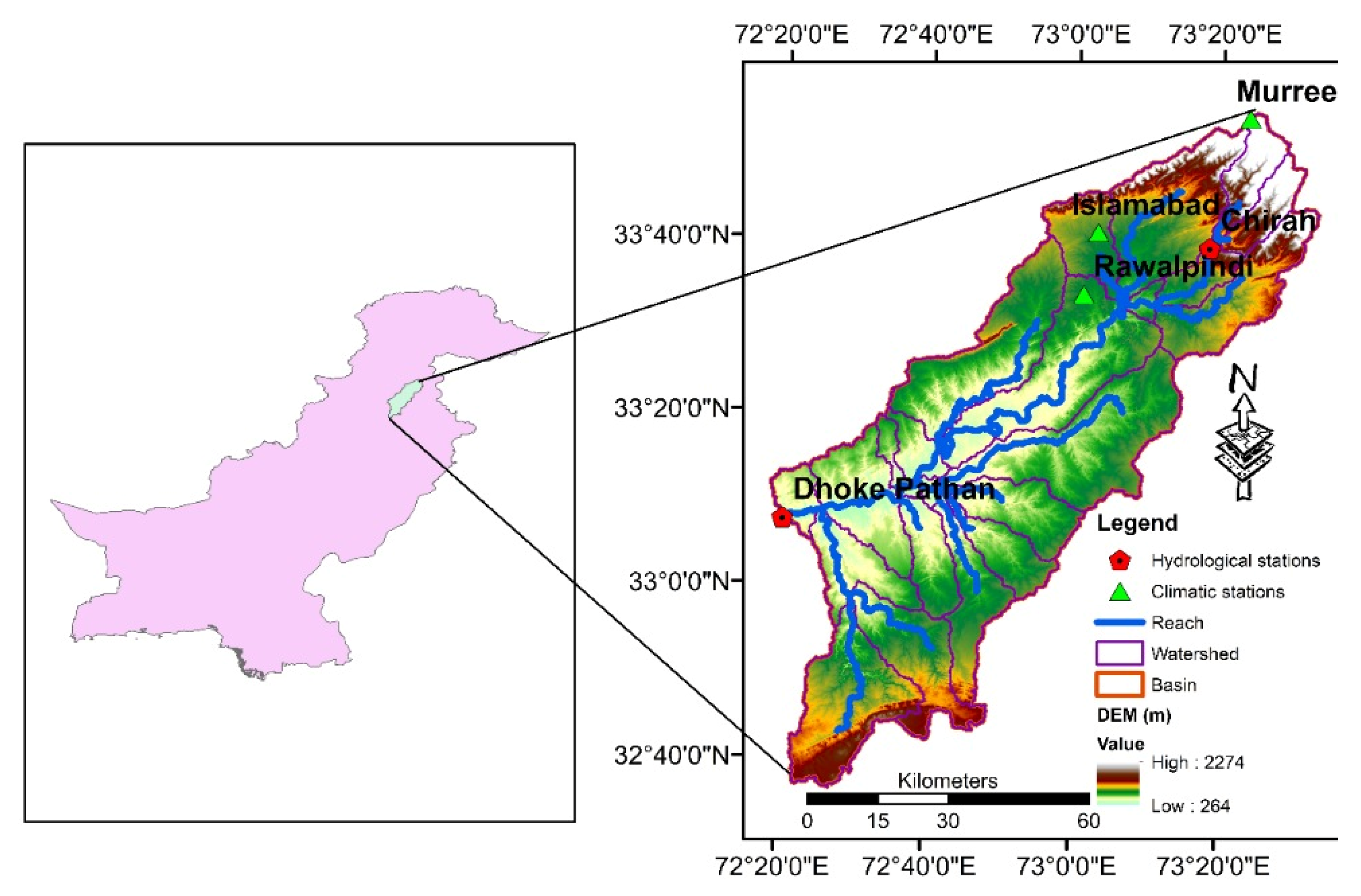
The Soan River is a major tributary of the Indus River and a substantial supplier of water for the Pothwar regions of Pakistan [31]. It begins in Murree mountains and passes through two hydrological stations of Chirrah and Dhok Pathan before flowing into the Indus River. The SRB covers an area of 6842 km2 with maximum height of 2274 m. The average annual temperature in the SRB varies between 8–18 °C with average annual precipitation of 1465 mm. The northern area of the SRB has humid and sub humid climates whereas southern area has arid and semiarid climates [32]. Simly dam is also a major supplier of water for the capital city (Islamabad) that receive water from the SRB. Furthermore, the SRB significantly contributes to Pothwar’s agriculture and domestic water use. The slope of the SRB varies from gentle to steep, and monsoon season generates the majority of the stream flow. The study area’s population has grown dramatically in recent years owing to an increase in rural-to-urban migration, suggesting that water supplies are under persistent pressure [22].
2.2. Data Collection
2.2.1. Observed Climatic Data
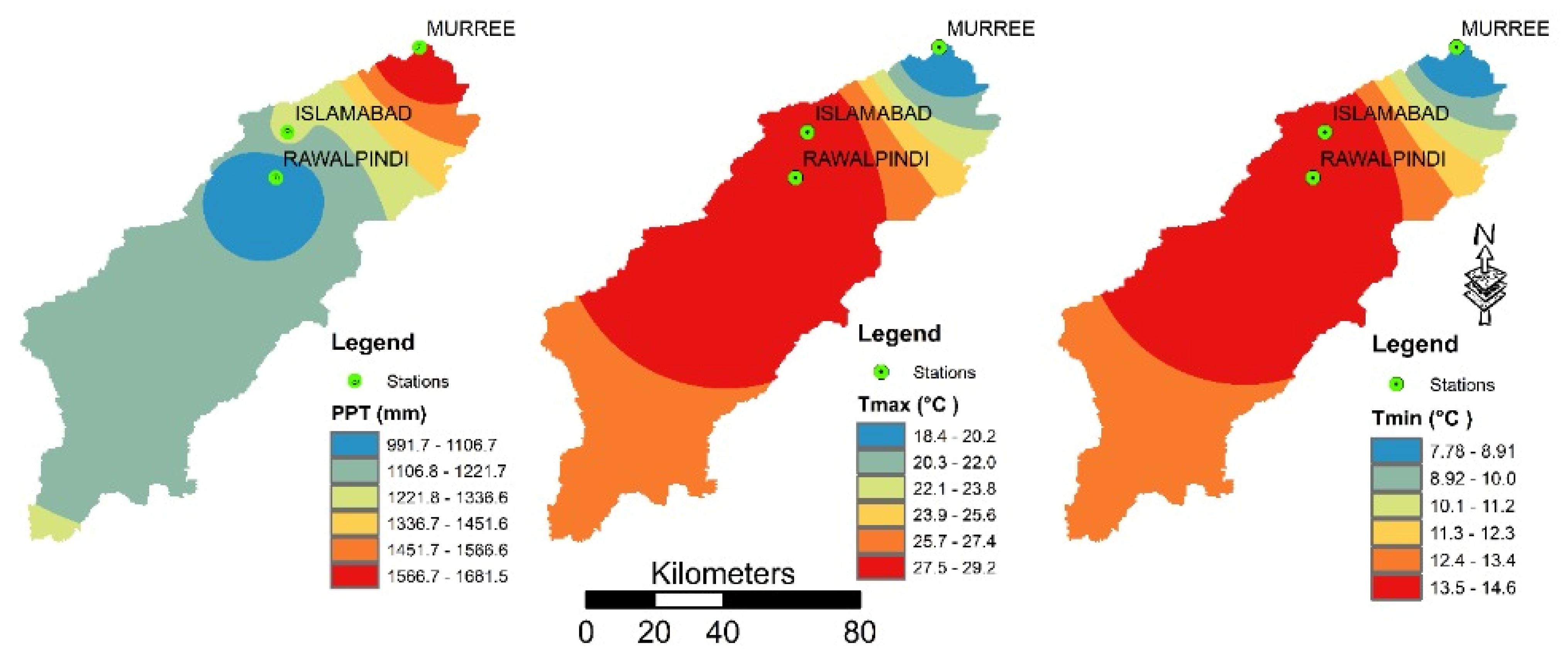
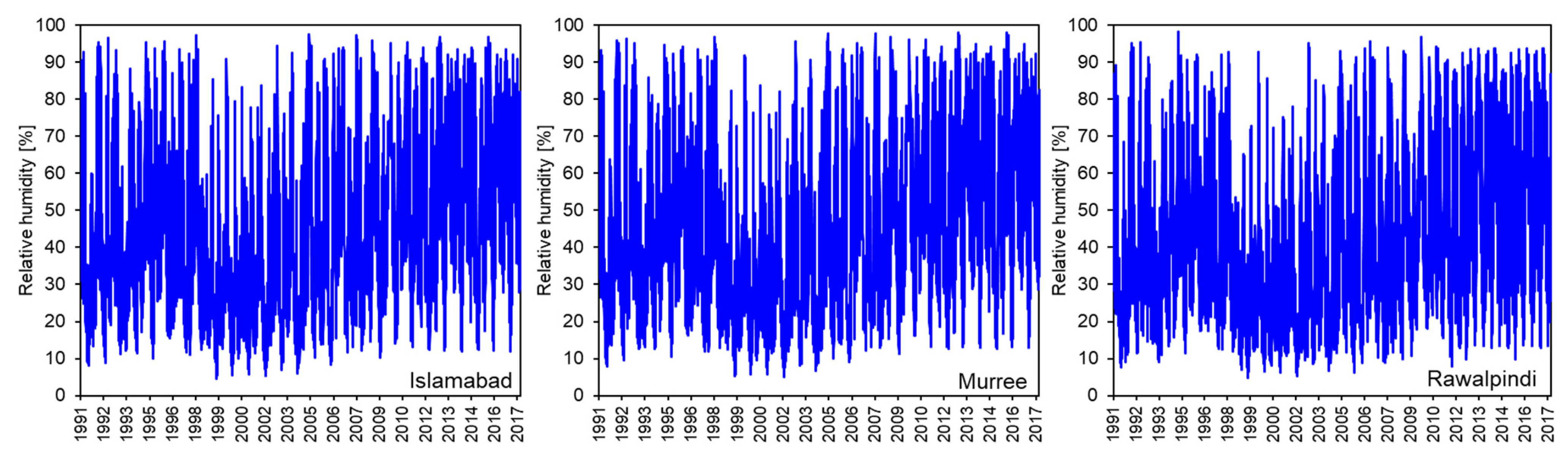
The study employed climatic data obtained from the Pakistan Meteorological Department and Soil and Water Conservation Research Institute for three meteorological stations, as shown in Figure 1, for the period of 1991–2017. The climatic data was obtained in terms of temperature, relative humidity, precipitation, wind speed, and solar radiation. The precipitation and temperature data are shown in Figure 2. However, the relative humidity, wind speed, and solar radiation data is available in Appendix A (Figure A1 and Figure A2). Stream flow data (gauged data) was collected from a hydrological station (Chirrah) of Water and Power Development Authority (WAPDA) only for the period of 2006–2013 due to the non-availability of long-term data.
2.2.2. Model Data
Model data including , , and precipitation were acquired for developing the CNRM-CM5 Model. The climatic projections were categorized into two groups such as the baseline period (1991–2005) and three future periods: early century (2021–2045), mid-century (2046–2070), and late century (2071–2095). Five global climate models (Access 1.0, CNRM-CM5, CCSM4, CSIRO, and MPI-ESM-LR) were used in this study, and the data was downloaded from reference [33].
2.2.3. Spatial Data
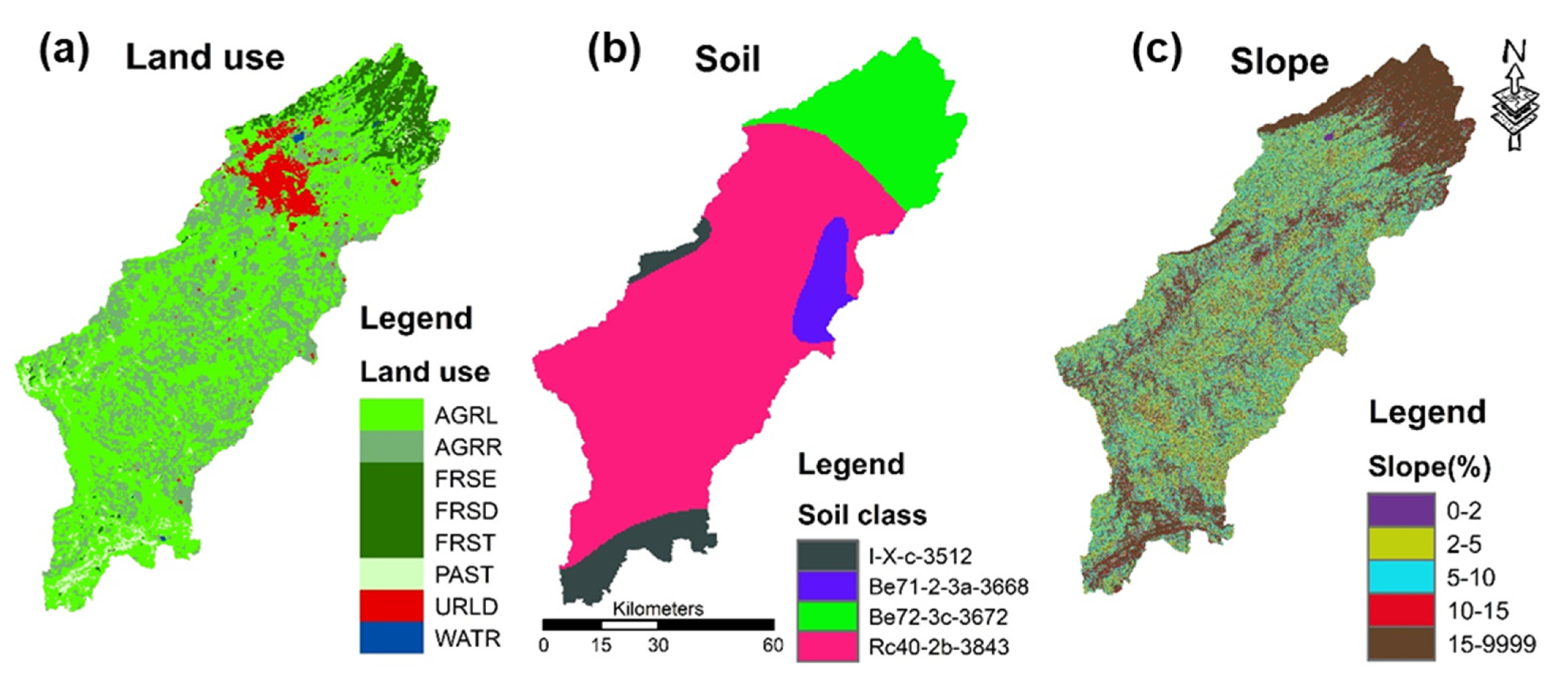
Spatial data comprising the digital elevation model (DEM), soil data, and land use (LU) data was incorporated into the SWAT model. The coordinate system used to project each spatial dataset was the same as WGS 1984 UTM ZONE 43N. The SWAT model developed the stream network plus defined the watershed using the DEM of the research area. It was purchased from the CGIAR-Consortium for spatial information v4.1 database (23). The LU data was collected from the National Engineering Service of Pakistan (NESPAK). After that, this LU data was categorized into eight classes including agricultural land generic, agricultural land-row crops, forest ever green, deciduous, mixed, pasture residential low density, and water, as shown in Figure 3a. The digital soil map of the world (DMSW) was utilized to download soil information from the reference [34]. The DEM data of the SWAT model defined five slope classes and soil classification in Figure 3b. The most central soil category is Gleyic Solonchaks, which covers 67.32% of the basin area. The dataset of soil classification for this region was obtained from the reference [34]. Based on the DEM data, the SWAT model defined five slope classes as shown in Figure 3c.
2.3. Climate Change Analysis and Downscaling
Linear scaling was applied to completely meet the corrected monthly average values with observed values [35,36,37]. Monthly variations in climatic data were obtained using observed data (1991–2017) and GCMs data. The following equations were used to predict future temperature and precipitation data of the GCMs using the bias correction method.
where and represents the observed monthly temperature (°C) and precipitation (mm), respectively, while and represents the raw data observed monthly temperature (°C) and precipitation (mm), respectively. represents a change in temperature (°C), represents temperature (°C), represents a change in precipitations (mm), and represents precipitation (mm). By using these above equations, climatic data was examined relative to baseline periods on a seasonal and annual basis for future possibilities. The predictions were divided into three future periods: early century (2021 to 2045), mid-century (2046 to 2070), and late century (2071 to 2095) while the selected baseline period was 1991 to 2017.
2.4. Bias Correction
In this study, two GCMs, Access 1.0, and CNRM-CM5, under two representative concentration pathways (RCPs) such as RCP-4.5 and RCP-8.5, were employed to predict the future impact of CC [14]. A statistical analysis including the 90th percentile, mean, standard deviation, and 10th percentiles was applied for non-bias corrected data, observed data, and for bias corrected data for , , and precipitations. Linear scaling was applied to completely meet the corrected monthly average values with observed values [35,36,37]. Monthly variations in climatic data were obtained using observed data (1991–2017) and GCM data. The bias correction of climatic parameters (precipitation, temperature) depended upon the below two equations.
where and represent bias corrected monthly precipitation and temperature, respectively. and represent the GCMs values for precipitation and temperature, respectively. and are the precipitation and temperature observed values, respectively. The and are GCMs historical simulated values of precipitation and temperature. The bias correction was done by adopting the following steps.
- The observed data period (1991–2010) was divided in to two groups: calibrated period (1991–2000) and validated period (2001–2010) for bias correction.
- For the calibration period, the correction factor for temperature and precipitation were calculated using historical data of the model and observed data.
- The linear scaling performance evaluation was estimated depending upon the evaluation of the 10th percentile, standard deviation, mean, and 90th percentile between two types of data (observed data, model data) formerly and later bias correction.
- The performance for the calibrated period was assessed after applying the bias corrected calibration period parameters to the validation period.
- The future forecasted model data of 2021–2095 was corrected monthly using the monthly correction factor.
2.5. SWAT Model for Hydrological Modelling
The study considered SWAT model to simulate the stream flow of watersheds because long-term simulations and predictions are possible with this model [38,39,40]. In a wide variety of watersheds, the SWAT model can replicate the stream flow process [35,41]. In various climate impact studies [42,43,44], the SWAT model shows promising results for simulating the long-term hydrological changes. Furthermore, these studies also concluded that the SWAT model is more efficient in the case of large catchments and provides satisfactory results, particularly for annually, daily, and monthly values. The SWAT model combined the spatial data, including soil data, land use, and digital elevation data. The DEM of the studied area was employed in the SWAT model to delineate the watershed and river network. The generated data were used to evaluate the hydraulic response unit (HRU), and each HRU simulates its own discharge at a monthly scale, which directed it to obtain total discharge from the entire watershed. The water balance equation is used to evaluate the hydrological parameters of the SWAT model [23,45].
where represents final soil water content (mm/day), represents initial soil water content (mm/day), represents time (days), represents the amount of precipitation (mm), represents the amount of surface runoff (mm), represents the amount of evapotranspiration (mm), represents the amount of percolation (mm), and represents the amount of return flow (mm).
2.5.1. Calibration and Validation
The calibration of the model is the process of changing parameter values to ensure that the developed or simulated model flow accurately represents the changes of actual flow [46]. To acquire a better alignment between simulated and observed data (gauged data 2006–2009), calibration was achieved utilizing manual calibration as well as SWAT adjustment and an uncertainty program using SWAT-CUP (SWAT Calibration Uncertainty Program). In this regard, outflow from the SRB is simulated using ArcSWAT. Monsoon season starts in Pakistan from July to September, so runoff was found at maximum value in this season while the driest period of this region was from November to December. Data from GCMs was utilized as inputs for the SWAT model, which resulted in a variety of runoff series (6-time series and one baseline data). These six-time series belong to GCMs and given future conditions. The SWAT model generates replicate runoff data above its sub basin to determine CC impact. The same method has been successfully utilized by different studies [47,48,49].
2.5.2. Performance Evaluation
The SWAT model’s performance was assessed based on the most commonly used parameters such as the coefficient of determination (R2), percent bias (PBIAS), and Nash Sutcliffe Efficiency (NSE). The R2 values from 0 to 1 indicates that either simulated and observed data are correlated or not. Higher values of R2 (normally > 0.5) represent greater correlation with less error. The NSE represents how precisely the simulated plots turn the measured plots. It varies between 0 to 1, and values greater than 0.5 are regarded as acceptable if the model shows less error at higher levels. The PBIAS shows percent mean divergence between simulated and actual flows and might have a positive or negative value. The PBIAS values varied between −15 to +15 are considered acceptable [50].
3. Results
3.1. Climatic Model Selection
The climatic model was selected based on the observed values of R2 for selected GCMs (Access 1.0 and CNRM-CM5). The results showed that the R2 for Access 1.0 and CNRM-CM5 were 0.34 and 0.43, 0.31 and 0.52, and 0.47 and 0.35 at Rawalpindi, Islamabad, and Murree metrological stations, respectively. While the other three GCMs (CCSM4, CSIRO, and MPI-ESM-LR) give a lower value of R2. The climatic parameter precipitation was selected for comparison with GCMs data from 1991–2005. The values of these three GCMs are given in a table below. It was observed that the CNRM-CM5 performed well as compared to the other four GCMs models on the basis of a high value for the coefficient of determination R2. A high value for R2 for CNRM-CM5 was due to more precipitation data similarity with a baseline precipitation as compared to Access 1.0 and the other three models. In this regard, the CNRM-CM5 model was selected for evaluation impact of CC on the SRB.
3.2. Bias Correction
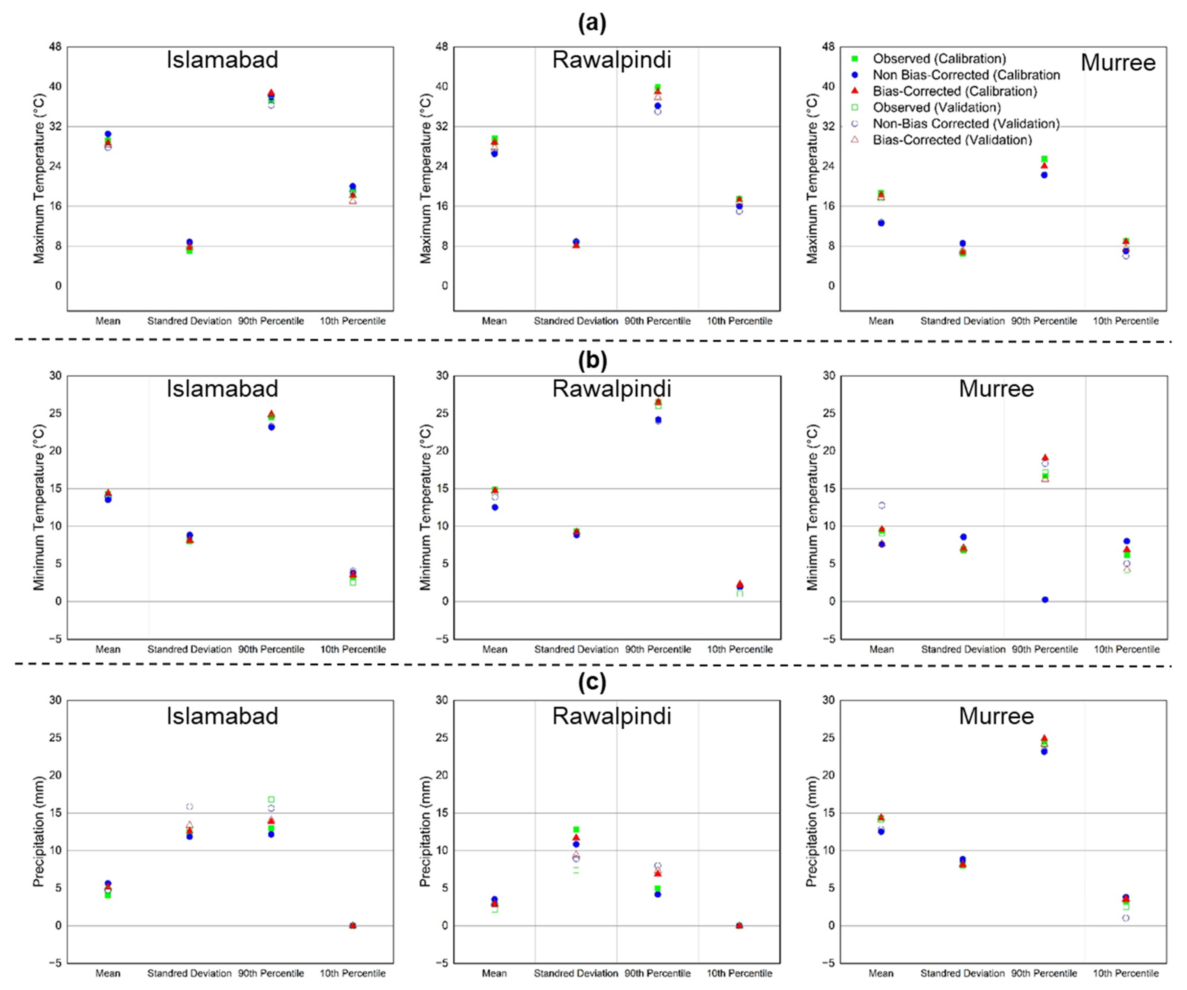
A statistical analysis including the 90th percentile, mean, standard deviation, and 10th percentiles was applied for non-bias corrected data, observed data, and for bias corrected data for , , and for precipitation at meteorological stations of Rawalpindi, Islamabad, and Murree as shown in Figure 4. The correction factor established during the calibration period (1991–2000) was useful to the validation period (2001–2010). During bias correction, a correction factor in the calibration period of 1991–2000 was found, thereby utilized for validation period of 2001–2010. Additionally, a performance evaluation of both periods was calculated. According to the results, the calibration period increased more than the validation period at each meteorological station. The standard deviation, mean, and 90th percentiles showed underestimated results for , , and precipitations at the selected metrological stations using non-bias corrected signs. However, the bias corrected and observed mean precipitation results become equal during the calibration period at all metrological stations while the percentage difference of 51.5%, 41.9%, and 18.26% was observed at Rawalpindi, Islamabad, and Murree station, respectively, as compared to the observed results. For the , the signs showed both underestimated and overestimated results mostly in the case of non-bias corrected data for both the calibration and validation periods for Murree and Rawalpindi station, while for Islamabad station, the signs show very little variations. In the case of Murree station, the mean values percentage difference for the was observed at −38.76% (non-bias corrected) during the calibration period while at −37.12% during the validation period. However, in the case of the 90th percentile, the percentage difference for Murree station was improved from 16.91% during the calibration period and 5.77% during the validation period with respect to the observed data. The percentage difference for the 10th percentiles was improved −23.11% during the calibration period and −2.18% during the validation period according to observed data for Murree station. The non-bias adjusted data for the , which includes the mean, 10th percentile, and 90th percentile, reveals overestimated and underestimated values for the calibration and validation period at all climatic stations. At Murree station, for , the percentage difference for the 90th percentile is 4.50% for non-bias correction and 9.50% for bias correction with respect to the observed data. Generally, it was detected that linear scaling applications meaningfully enhanced the statistical signs at all climatic stations. This demonstrates how effective these strategies are at improving the output of the chosen CNRM-CM5 model for the study area.
3.3. Assessment of Mean Monthly Future Meteorological Parameters at Climatic Stations
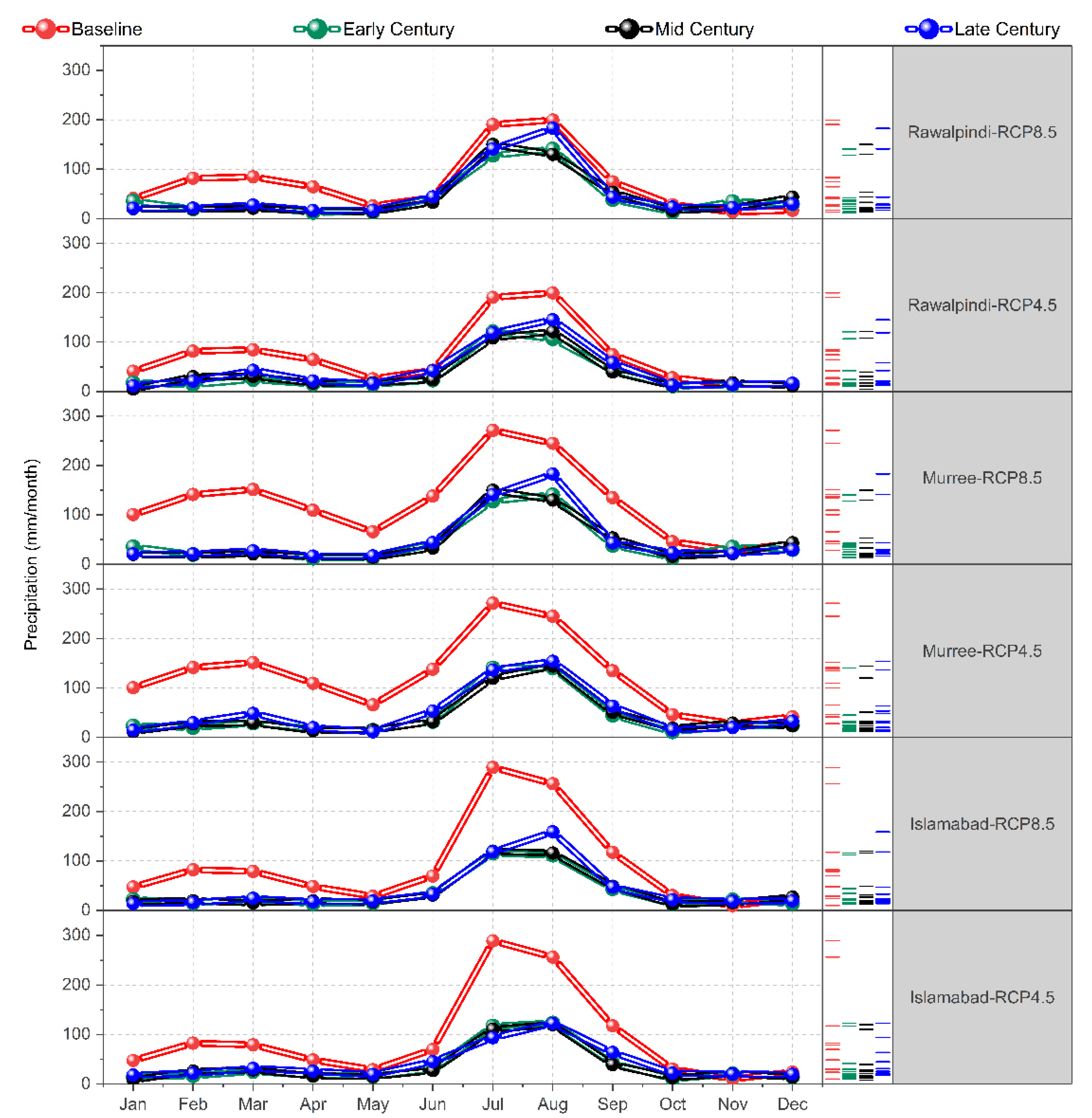
The mean monthly future meteorological parameters like precipitation, , and were evaluated for the observed baseline period (1991 to 2017) and forecasted for early (2021 to 2045), mid (2046 to 2070), and late century (2071 to 2095) using the CNRM-CM5 model under both RCP-4.5 and RCP-8.5 for selected stations. Figure 5 represents the fundamental mean monthly profiles of precipitation for the base line period, early century, mid-century, and late century under RCP-4.5 and-RCP-8.5 at selected stations. In the case of both actual and prospective timeframes, the predicted peak precipitation levels were observed in July and August at selected stations under both emissions scenarios. In the case of mid-century (except Murree RCP-4.5), the maximum difference in precipitation was predicted to be between 127 mm/month and 155 mm/month for the month of July under both RCP-4.5 and RCP-8.5 while there is relatively minor change in precipitation between early and late century under both RCPs at selected stations. Additionally, in case of the Islamabad climate station, it was predicted that there will be more precipitation in the month of July rather than August. The early century was predicted to experience high precipitation of 200 mm/month which is approximately 50.90% higher than the baseline period under RCP-4.5. However, the mid- and late century were predicted to experience about 28% and 36% less precipitation than the baseline period. The precipitation in the early century under RCP-8.5 was predicted to be less than RCP-4.5 but still 45% less than the baseline period. Similarly, the predicted results of other stations can be found in Figure 4.
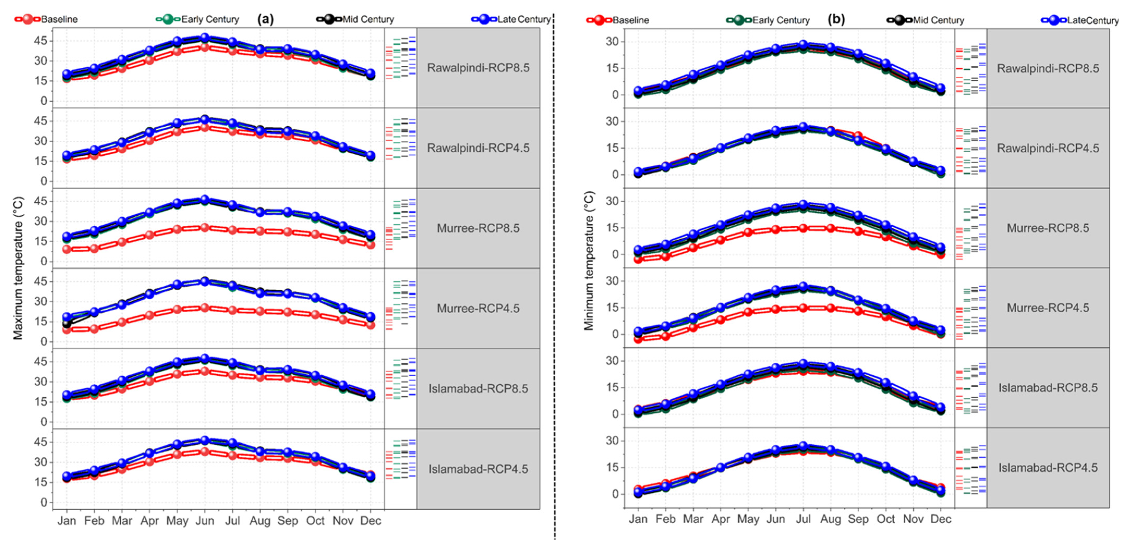
Figure 6 represents the monthly profiles of and for the base line period, early century, mid-century, and late century under RCP-4.5 and RCP-8.5 at selected stations. The was observed in the month of June in the case of early and mid-century for selected stations under both RCP-4.5 and RCP-8.5 as shown in Figure 6a. The early and mid-century was predicted to be greater than the baseline period, and this increment is observed to be significantly higher under RCP-8.5 as compared to RCP-4.5. However, in early and mid-century, a minor temperature difference was observed under RCP-4.5 but about 34.57% greater as compared to the baseline period for selected stations.
Consequently, in the case of Islamabad, the of 42.5 °C was observed in the month of June for the late century under RCP-8.5 which is 3.5 °C or 26% greater as compared to the baseline period of 38 °C while of 42.5 °C was observed in the same period under RCP-4.5. However, in early and mid-century, under RCP-8.5 was approximately equal to the temperatures under RCP-4.5. According to Figure 6b, the highest values of were in the month of July for all time periods and stations under both emission scenarios. In the case of Islamabad, highest value of of 28.5 °C was observed in the late century for the month of July as compared to the baseline period of 24 °C under RCP-8.5 while according to RCP-4.5, the highest value of of 27 °C was observed.
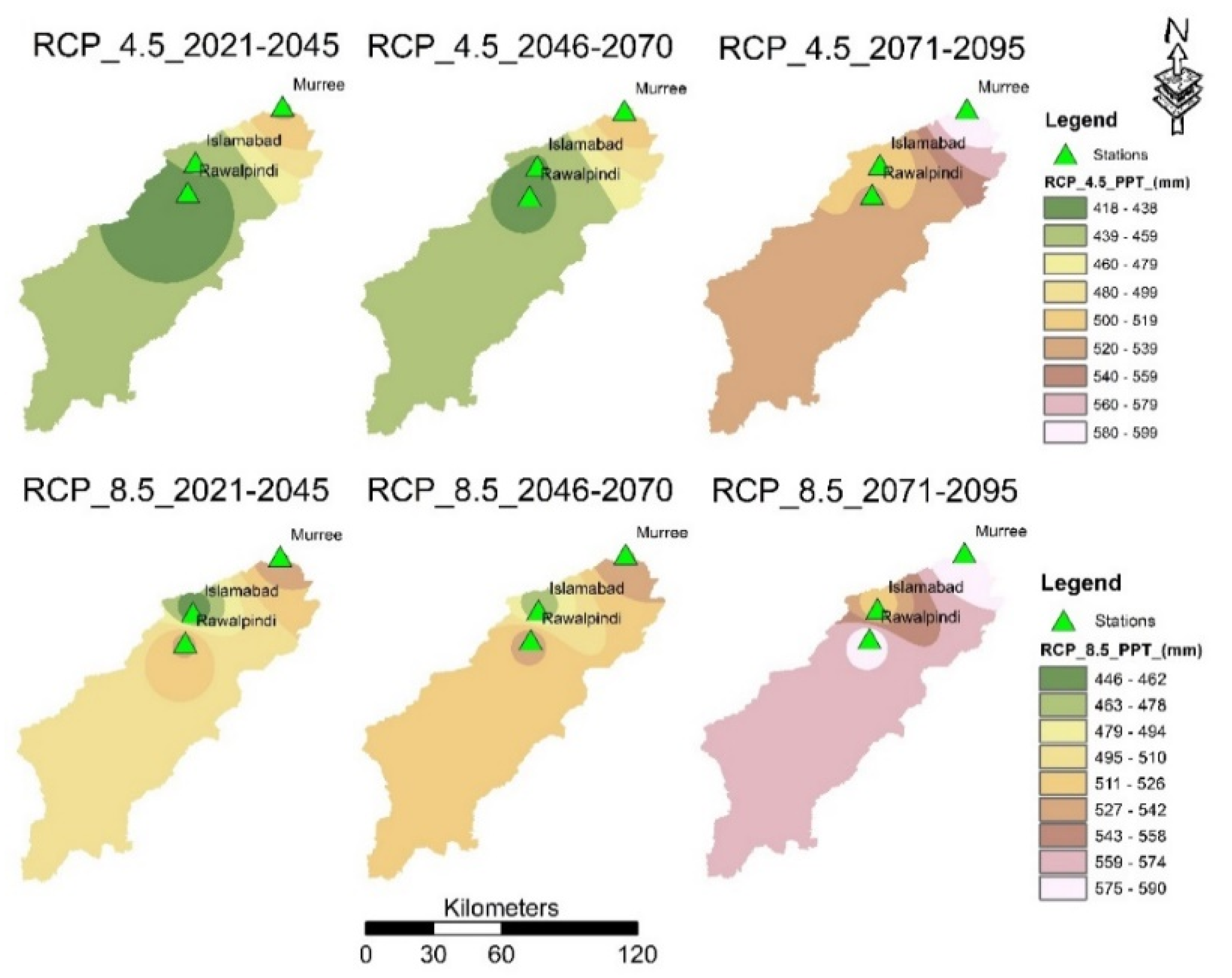
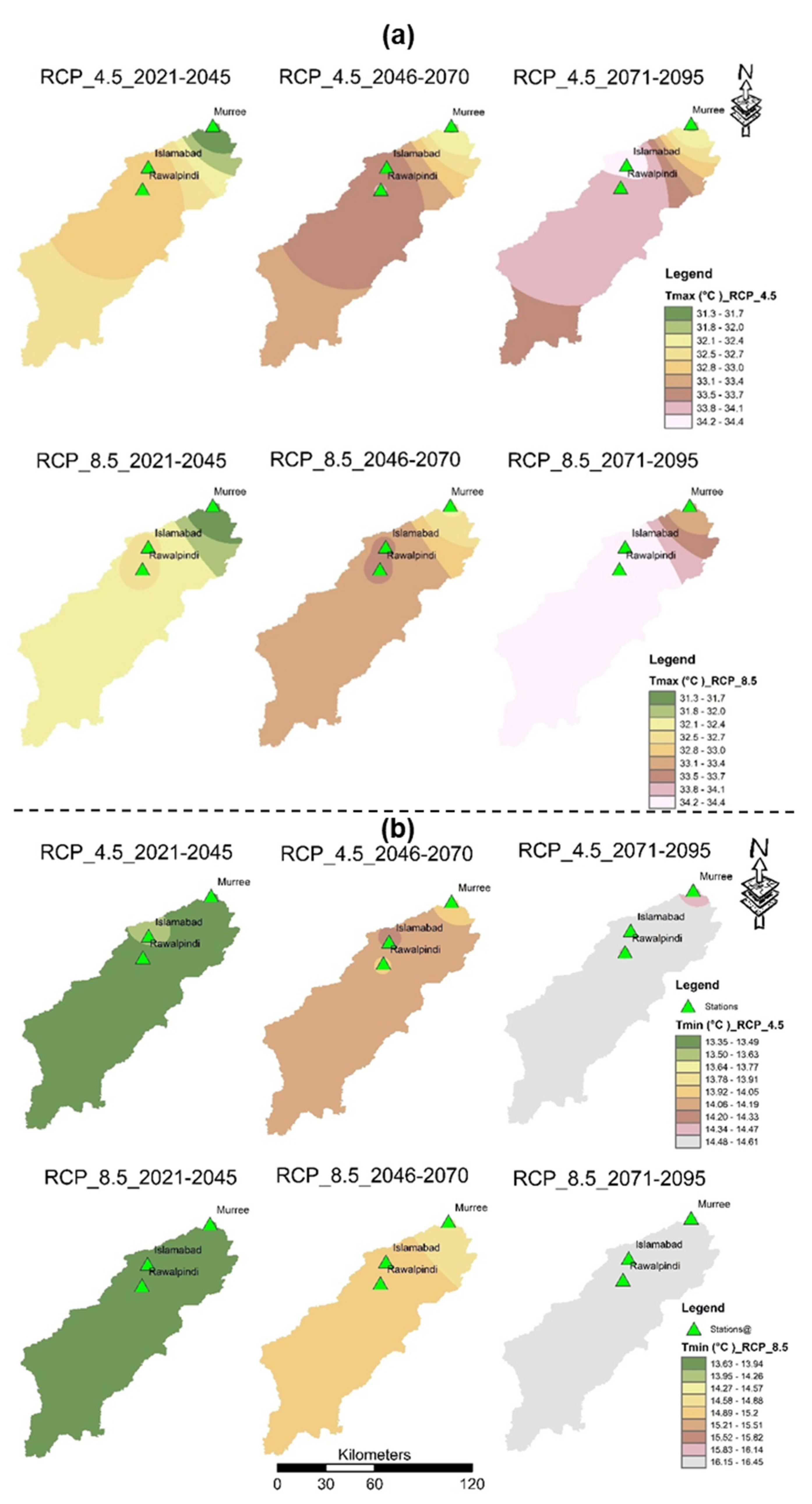
Additionally, for more clarification, the spatial distribution of the precipitation data in the SRB for early, mid, and late century under both RCP-4.5 and RCP-8.5 is represented in Figure 7. It is observed that the annual average precipitation is going to decrease from the early to late century. Similarly, Figure 8 represents the spatial distribution of and data in the SRB for early, mid, and late century under both RCP-4.5 and RCP-8.5. Figure 8a shows spatial distribution of in the SRB for early, mid, and late century under both RCP-4.5, and RCP-8.5. It was observed that varied between 31.4 °C to 34.4 °C under both RCP-4.5, and RCP-8.5. Similarly, Figure 8b shows spatial distribution of in the SRB for early, mid, and late century under both RCP-4.5, and RCP-8.5. It was observed that varied between 13.4 °C to 14.6 °C under RCP-4.5 while 13.6 °C to 16.5 °C under RCP-8.5. The results conclude that and will increase from early to late century which will result in a serious water threat in the near future.
According to Ikram et al. [51], the projected precipitation increases in Pakistan and is expected to be 2–3 mm/day under RCP-4.5 while 3–4 mm/day under RCP 8.5. The temperature increases were predicted to be 3 °C to 4 °C under RCP-4.5 and 3 °C to 8 °C under RCP-8.5. The findings of this study showed similar trends in temperature, but due to the use of different GCMs, precipitation showed a slight variation. In a previous study by Babur et al. [28], the change in , , and precipitation in Pakistan was varied from (−50) to (+70%), 3 °C to 6 °C, and 2.5 to 8 °C, accordingly, in RCP-4.5 and 8.5. The current study facts by Babur et al. show that extreme temperature shows a little variation while precipitation within the projected limit [28]. This might be due to a different GCM for climate prediction. Because of different study areas, several climate models can propose various outcomes. Naeem et al. [52] studied the impact of CC on the hydrological regimes of Jhelum River Basin and observed an annual increase in , , and precipitation of 0.4–4.18 °C and 0.3–4.2 °C and 1–1.4 mm and 2.1–2.8 mm under RCP-4.5 and 8.5, respectively [52]. Islam et al. [30] investigated the climatic and hydrological changes on the upper Indus River and found a significant increase in temperature and a decrease in precipitations [30]. Mahmood et al. [53] found an increase of 12% to 14% in precipitation at the end of this century at Jhelum River basin [53]. Shaukat et al. [54] concluded that there is a 0.5–2 °C increase in the temperature at the upper Indus basin system [54].
3.4. Water Balance/Stability in SWAT Model
Table 1 represents the water stability for the baseline period in a simulated hydrological SWAT model. Inflows and outflows were almost equal excluding a little difference because of losses happening in the watershed. About 59% of the inflows were used to produce water, which showed that the streamflow was being affected by most of the precipitation.
3.5. Calibration and Validation of the SWAT Model
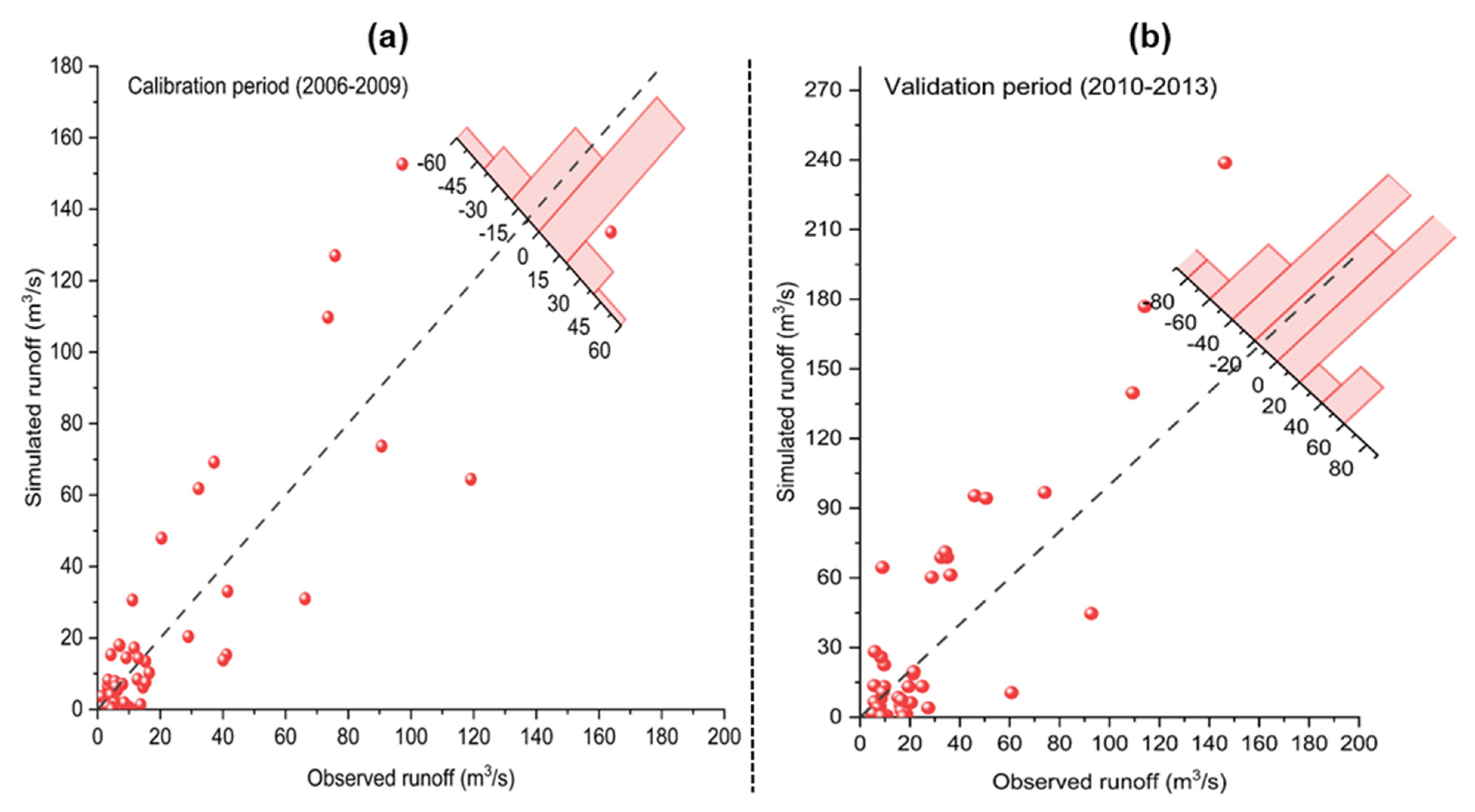
Observed data collected by WAPDA at Chirrah gauge station on the SRB was employed for the calibration (2006–2009) and validation (2010–2013) of the SWAT model as shown in Figure 9. Twelve parameters were measured from which five were considered comparatively sensitive as shown in Table 2. Additionally, Table 3 shows the annual average water balance for the SRB (1991–2017). In Table 4, using the available information and the predicted results, the SWAT model simulation’s effectiveness was assessed from the viewpoints of R2, PBIAS, and NSE are presented. To acquire complex parameters for calibration and validation, previous research work was the main point of concentration [37,55,56]. Five model parameters, which include Curve Number (CN), Groundwater Recharge Evaporation (GWRE), Soil Evaporation Compensation (SEC), Soil Available Water Capacity (SAWC), and slope, were adjusted to simulated results similar to the actual values. It was observed that all sub watersheds increased four-fold in the case of the CN while the GWRE was accepted as 0.4 and SEC was increase by 0.8, and SAWC and slope parameters multiplied by 0.4 and 1.3, respectively. This shows that for this particular watershed, factors relating to soil processes, surface runoff, and groundwater processes have the greatest effects on the output of the SWAT. The detailed explanation of every parameter of this model is available in user’s manual of the SWAT [57].
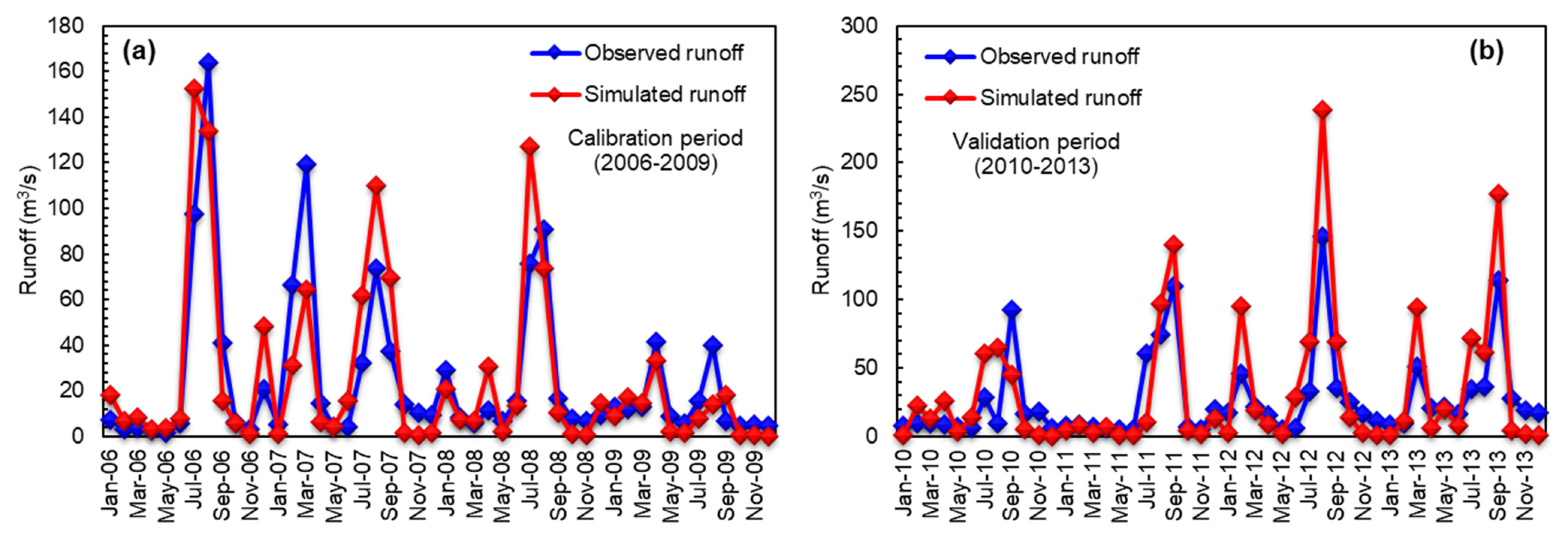
Figure 10 shows the profiles of simulated and observed runoff at the SRB for the calibration and validation periods. It was observed that simulated runoff during the calibration period was greater from July 2006 to September 2008 while lower values were observed from January 2006, May 2006, and November 2008 to December 2009. However, in case of the validation period, the simulated flow was observed less from June 2010 to June 2011 while higher values were observed between May 2012 and August 2012. The variations in runoff data are due to different precipitation data observed and calculated with the GCM at all selected stations.
3.6. Prediction of Streamflow Variations
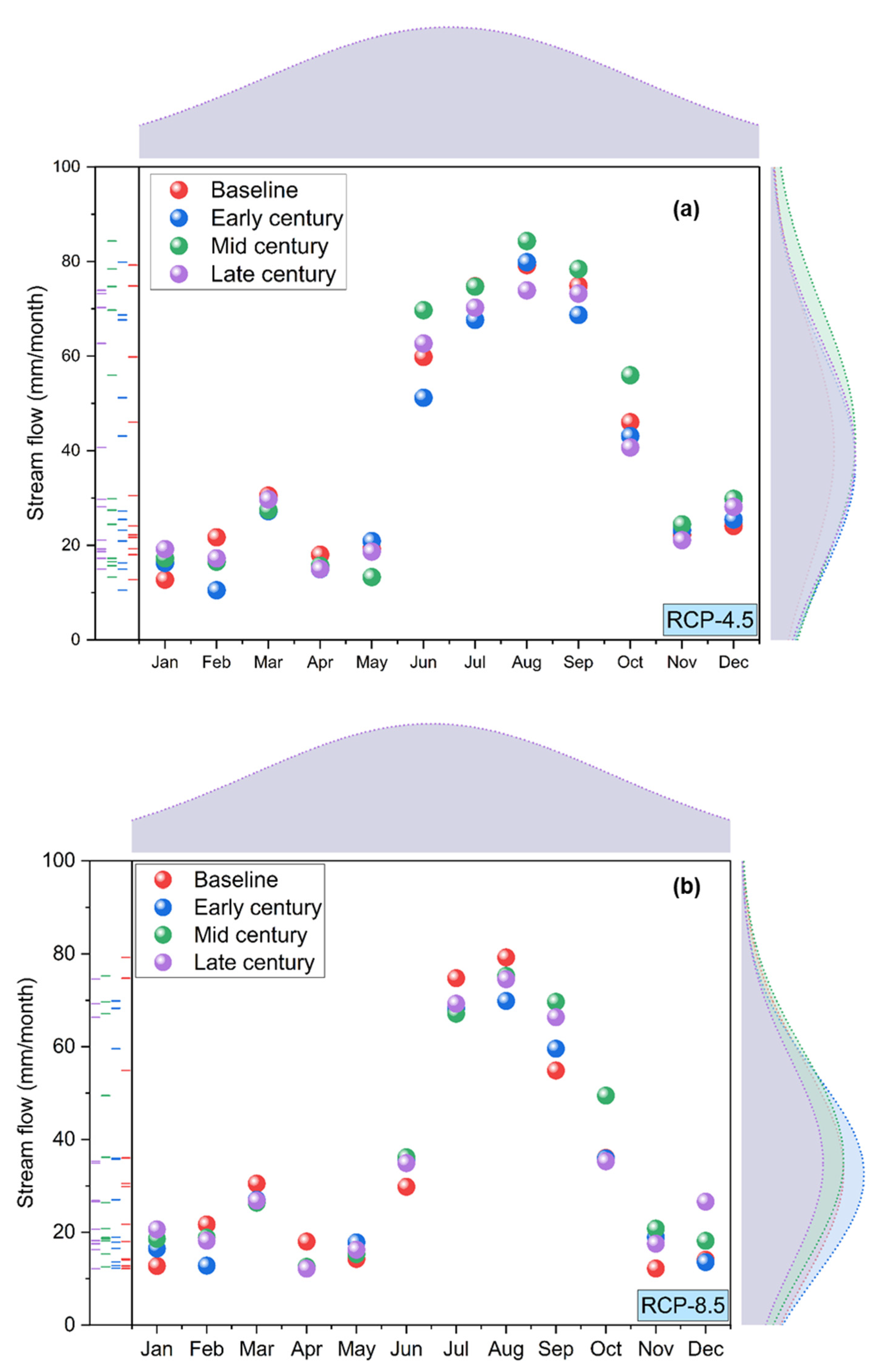
Figure 11 shows monthly changes in stream flows for the baseline to late century with their marginal distribution curves in the SRB under both RCP 4.5 and RCP 8.5. The predicted monthly stream flows were observed at a maximum of 84.34 mm/month and 78.41 mm/month from July to August under RCP-4.5 as shown in Figure 11a while 67.12 mm/month and 75.25 mm/month under RCP-8.5 as shown in Figure 11b in the mid-century period for selected stations. It is important to mention here that the marginal distribution curve in Figure 11 shows a data height in numbers instead of density or relative frequency of data. Additionally, in mid-century, the predicted annual averaged stream flows were observed at a maximum of 42.31 mm and 35.71 mm under RCP-4.5 and RCP-8.5, respectively. The significant difference was observed in peak runoff established in the late century under both emission scenarios. At all meteorological stations, the trend of mean monthly precipitation was directly related to the trend of stream flow.
4. Discussion
In general, a hydrological model and climate simulations by GCMs, which are run in future under various RCPs, must be combined in order to assess the hydrological implications of CC [58]. The parameters such as precipitation, , , relative humidity, and wind speed are major variables for hydrological presentations in particular, hence stream flow forecasting/projections depends on accurate data for these variables at the catchment size. Numerous features of climatic variables are measured using several metrics, such as the 90th percentile, mean, standard deviation, and 10th percentile for both bias and non-bias corrected data of climatic variables for future prediction, which was divided into three future periods of early (2021–2045), mid (2046–2070), and late century (2071–2095). In order to estimate how effectively the CNRM-CM5 model simulates the observed data over the research area, for one sub catchment of (SRB) in Pakistan, these measures were initially utilized. Additionally, relatively minor variations in climatic variables may result in significant variations in the future prediction of climate variables [59,60,61].
Therefore, the SWAT model’s calibration and validation was done to anticipate streamflow across the Chirrah sub catchment. When measured against a particular objective function, the model’s performance during calibration is typically effective since it highlights a specific system characteristic [62]. However, concurrently, other system characteristics may experience significant faults [63]. While evaluating the performance of hydrological model using various objective functions takes into account the various uncertainties that may be present in a system, a representative set of Pareto optimum results of the model’s parameter is produced as a result avoiding simulation from being biased near one objective function and specifying an exclusive solution that can increase or decrease a specific independent priority [64,65]. For example, the NSE illustrates how large the residual variance is in comparison to the variance of the observations and could lead to an incorrect assessment of the model’s performance [66]. In this work, the performance of the SWAT model was evaluated during autonomous calibrated and validated periods using a variety of objective functions, including R2, PBIAS, and NSE. These centuries were carefully chosen to account for the future forecasting of climate variables, thus reducing inaccuracies [66].
The SWAT model worked exceptionally well during the calibrated and validated periods for Chirrah sub catchment in (Figure 10); this model has also done exceptionally well in other catchments with utterly dissimilar characteristics, such as complicated terrain [28]. The small PBIAS (%age transformation between gauged and modeled streamflow) values suggest the strength of the model’s factors, which is very suitable for sub catchment. The divergence between gauged and modeled runoff during the calibrated and validated periods is a reflection of the inaccuracies in model arrangement and factors values [67]. For the investigation on the implications of climate change, the choice of appropriate GCMs is crucial [68]. For this, the runoff for the historic period of 1991–2017 was initially simulated by means of both gauged and modeled (CNRM-CM5) climatic data for Chirrah sub catchment by means of the SWAT model (after calibration and validation). The streamflow for the early century (2021–2045), mid-century (2046–2070), and late century (2071–2095) future periods was than simulated by means of the climate data from CNRM-CM5, enforced with two emission scenarios of RCP-4.5, and 8.5.
The best GCM across the sub catchment was chosen after R2 was used to access the GCMs appropriateness for streamflow modeling [69]. The average minimum and maximum temperature was found to be increased from 1.31 °C to 4.67 °C from early to late century, and a decrease in precipitation was found to be 43.86 mm to 86.86 mm from early to late century; that is very close to the previous studies value while precipitation shows a slight variation [28,51]. Performance evaluation parameters like R2, PBIAS, and NSE also give satisfied values: 0.81, −0.87, and 0.78 for calibration period and 0.83, −0.92, and 0.6 for validation period of the SWAT model. The value of NSE is little in validation but is justified due to area characteristics and comparable to the other studies like Baber et al.; in his study, he found the validation value was 0.65 for R2 and 0.55 for NSE [28].
5. Conclusions and Recommendations
The study evaluated the impact of CC on streamflow at SRB, which is the main tributary of the Indus River and a significant source of water for Pothwar regions of the country. The study concludes that bias in climatic parameters (temperature and precipitation time series) can be effectively removed using the linear scaling practices. After bias was corrected, and the statistical indicators significantly outperformed the observed time series. The SWAT was a useful tool for analyzing the water balance components since it accurately represented the hydrology for data scarce and high elevation regions. The results of the study showed that under both RCPs for early, mid, and late parts of the century, precipitation was predicted to decrease in the future. Winter was projected to be relatively dry while summer was predicted to get the most precipitation. Early June was also anticipated to have the highest and in comparison to the baseline period. The future rise in the was more significant than the . Furthermore, the runoff at the SRB was expected to decrease in the future, especially in the summer months (July and August) under RCP-8.5. The conservation of water may be useful during the high flow season to meet the demands in the dry season or low flow season. Indeed, the runoff is decreasing in the future; however, this increment may speed up the soil erosion process, which would lead to the reduction of the storage capacity of the Simly Dam.
The SRB is a key source of domestic water supplies for Rawalpindi and Islamabad. Therefore, coordination is required between the various departments: Capital Development Authority, Rawalpindi Cantonment Board (RCB), and Water and Sanitation Authority (WASA). In addition, future research can be planned with the use of the SWAT model to predict sediment and runoff by studying LU changes. This study could help to cope with the reservoir storage capacity problem and promote effective maintenance techniques. Furthermore, as forecasted above, the effective rainfall will decrease while the average , and will increase in upcoming decades, ultimately leading to a reduction in freshwater resources and an increase in crop water demands. Therefore, there should be a strong relationship between the water management board and research institutes of the country to deal with the problems associated with water shortage.
6. Limitations
Short term discharge data for only eight years made the SWAT model calibration and validation challenging. However, the satisfied values of performance evaluation parameters (i.e., R2, PBIAS, and NSE) showed better performance. In this study, LULC was supposed to be persistent. In future studies, it is advised to consider how variations in LULC may contribute to CC. In conclusion, using a single GCM to evaluate CC forecasts into future flow projection has inherent vagueness. To better convey the future climate uncertainty, future work should include the whole group of GCM model outputs.
Author Contributions
Conceptualization, M.I. and G.P.; methodology, M.I. and G.P.; software, M.I. and E.A.; writing original draft preparation, M.I. and G.P.; validation, G.P., M.S., M.I. and M.A.; formal analysis, M.I., G.P. and R.X.; investigation, M.I., M.S., E.A. and F.U.K.; resources, G.P.; data curation, M.A., M.S. and M.I.; review and editing, M.S., G.P., E.A. and M.A.; visualization, M.I., G.P., M.S. and M.A.; supervision, G.P.; funding acquisition, G.P.; project administration, G.P. All authors have read and agreed to the published version of the manuscript.
Funding
This work was funded by the National Natural Science Foundation of China (Grant No. U2243211).
Institutional Review Board Statement
Not applicable.
Informed Consent Statement
Not applicable.
Data Availability Statement
The data are contained within the article.
Acknowledgments
This work is a part of the doctoral thesis of the first author Muhammad Ismail. This work is conducted at Northwest A&F University, 712100 Yangling, China under the supervision of Professor Gao Peng. This work was funded by the National Natural Science Foundation of China (Grant No. U2243211).
Conflicts of Interest
The authors declare no conflict of interest.
Appendix A
Figure A1.
Temporal relative humidity profiles of baseline period for Islamabad, Murree, and Rawalpindi.
Figure A1.
Temporal relative humidity profiles of baseline period for Islamabad, Murree, and Rawalpindi.

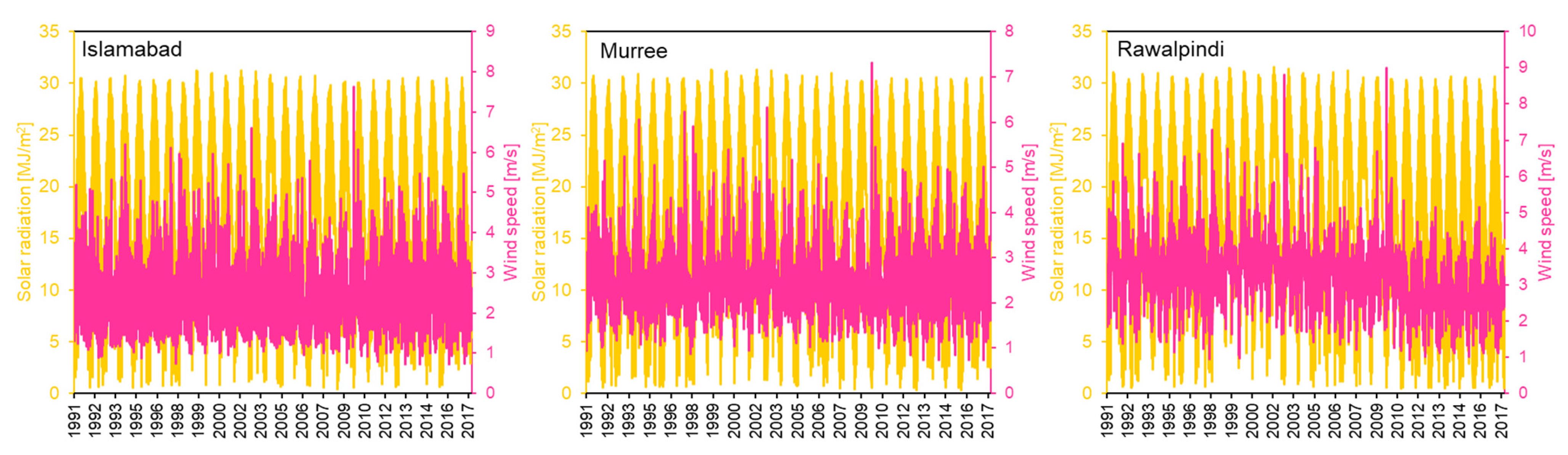
Figure A2.
Temporal solar radiation and wind speed profiles of baseline period for Islamabad, Murree, and Rawalpindi.
Figure A2.
Temporal solar radiation and wind speed profiles of baseline period for Islamabad, Murree, and Rawalpindi.

References
- Stocker, T. Climate Change 2013: The Physical Science Basis: Working Group I Contribution to the Fifth Assessment Report of the Intergovernmental Panel on Climate Change; Cambridge University Press: Cambridge, UK, 2014. [Google Scholar]
- Moser, S.C. Communicating Climate Change: History, Challenges, Process and Future Directions. Wiley Interdiscip. Rev. Clim. Change 2010, 1, 31–53. [Google Scholar] [CrossRef]
- Gosling, S.N.; Arnell, N.W. A Global Assessment of the Impact of Climate Change on Water Scarcity. Clim. Change 2016, 134, 371–385. [Google Scholar] [CrossRef] [Green Version]
- Pörtner, H.-O.; Roberts, D.C.; Adams, H.; Adler, C.; Aldunce, P.; Ali, E.; Begum, R.A.; Betts, R.; Kerr, R.B.; Biesbroek, R. Climate Change 2022: Impacts, Adaptation and Vulnerability. IPCC Sixth Assess. Rep. 2022. Available online: https://report.ipcc.ch/ar6/wg2/IPCC_AR6_WGII_FullReport.pdf (accessed on 6 September 2022).
- Akbar, H.; Nilsalab, P.; Silalertruksa, T.; Gheewala, S.H. Comprehensive Review of Groundwater Scarcity, Stress and Sustainability Index-Based Assessment. Groundw. Sustain. Dev. 2022, 18, 100782. [Google Scholar] [CrossRef]
- Tansar, H.; Akbar, H.; Aslam, R.A. Flood Inundation Mapping and Hazard Assessment for Mitigation Analysis of Local Adaptation Measures in Upper Ping River Basin, Thailand. Arab. J. Geosci. 2021, 14, 2531. [Google Scholar] [CrossRef]
- Milly, P.C.D.; Dunne, K.A.; Vecchia, A.V. Global Pattern of Trends in Streamflow and Water Availability in a Changing Climate. Nature 2005, 438, 347–350. [Google Scholar] [CrossRef]
- Urrutia, R.; Vuille, M. Climate Change Projections for the Tropical Andes Using a Regional Climate Model: Temperature and Precipitation Simulations for the End of the 21st Century. J. Geophys. Res. Atmos. 2009, 114, 1021. [Google Scholar] [CrossRef]
- Aziz, M.; Khan, M.; Anjum, N.; Sultan, M.; Shamshiri, R.R.; Ibrahim, S.M.; Balasundram, S.K.; Aleem, M. Scientific Irrigation Scheduling for Sustainable Production in Olive Groves. Agriculture 2022, 12, 564. [Google Scholar] [CrossRef]
- Ahamed, M.S.; Sultan, M.; Shamshiri, R.R.; Rahman, M.M.; Aleem, M.; Balasundram, S.K. Present Status and Challenges of Fodder Production in Controlled Environments: A Review. Smart Agric. Technol. 2023, 3, 100080. [Google Scholar] [CrossRef]
- Mujtaba, A.; Nabi, G.; Masood, M.; Iqbal, M.; Asfahan, H.M.; Sultan, M.; Majeed, F.; Hensel, O.; Nasirahmadi, A. Impact of Cropping Pattern and Climatic Parameters in Lower Chenab Canal System—Case Study from Punjab Pakistan. Agriculture 2022, 12, 708. [Google Scholar] [CrossRef]
- Dibike, Y.B.; Coulibaly, P. Hydrologic Impact of Climate Change in the Saguenay Watershed: Comparison of Downscaling Methods and Hydrologic Models. J. Hydrol. 2005, 307, 145–163. [Google Scholar] [CrossRef]
- Maurer, E.P. Uncertainty in Hydrologic Impacts of Climate Change in the Sierra Nevada, California, under Two Emissions Scenarios. Clim. Change 2007, 82, 309–325. [Google Scholar] [CrossRef] [Green Version]
- Shahi, N.K.; Das, S.; Ghosh, S.; Maharana, P.; Rai, S. Projected Changes in the Mean and Intra-Seasonal Variability of the Indian Summer Monsoon in the RegCM CORDEX-CORE Simulations under Higher Warming Conditions. Clim. Dyn. 2021, 57, 1489–1506. [Google Scholar] [CrossRef]
- Gonzalez, P.; Neilson, R.P.; Lenihan, J.M.; Drapek, R.J. Global Patterns in the Vulnerability of Ecosystems to Vegetation Shifts Due to Climate Change. Glob. Ecol. Biogeogr. 2010, 19, 755–768. [Google Scholar] [CrossRef]
- Arora, V.K. Streamflow Simulations for Continental-Scale River Basins in a Global Atmospheric General Circulation Model. Adv. Water Resour. 2001, 24, 775–791. [Google Scholar] [CrossRef]
- Zhang, X.C.; Nearing, M.A. Impact of Climate Change on Soil Erosion, Runoff, and Wheat Productivity in Central Oklahoma. CATENA 2005, 61, 185–195. [Google Scholar] [CrossRef]
- Hulme, M.; Hossell, J.E.; Parry, M.L. Future Climate Change and Land Use in the United Kingdom. Geogr. J. 1993, 159, 131–147. [Google Scholar] [CrossRef]
- Chen, Y.; Xu, Y.; Yin, Y. Impacts of Land Use Change Scenarios on Storm-Runoff Generation in Xitiaoxi Basin, China. Quat. Int. 2009, 208, 121–128. [Google Scholar] [CrossRef]
- Fowler, H.J.; Blenkinsop, S.; Tebaldi, C. Linking Climate Change Modelling to Impacts Studies: Recent Advances in Downscaling Techniques for Hydrological Modelling. Int. J. Climatol. 2007, 27, 1547–1578. [Google Scholar] [CrossRef]
- Bae, D.-H.; Jung, I.-W.; Lettenmaier, D.P. Hydrologic Uncertainties in Climate Change from IPCC AR4 GCM Simulations of the Chungju Basin, Korea. J. Hydrol. 2011, 401, 90–105. [Google Scholar] [CrossRef]
- Liu, L.; Liu, Z.; Ren, X.; Fischer, T.; Xu, Y. Hydrological Impacts of Climate Change in the Yellow River Basin for the 21st Century Using Hydrological Model and Statistical Downscaling Model. Quat. Int. 2011, 244, 211–220. [Google Scholar] [CrossRef]
- Arnold, J.G.; Srinivasan, R.; Muttiah, R.S.; Williams, J.R. Large area hydrologic modeling and assessment part i: Model development1. JAWRA J. Am. Water Resour. Assoc. 1998, 34, 73–89. [Google Scholar] [CrossRef]
- Christensen, N.S.; Lettenmaier, D.P. A Multimodel Ensemble Approach to Assessment of Climate Change Impacts on the Hydrology and Water Resources of the Colorado River Basin. Hydrol. Earth Syst. Sci. 2007, 11, 1417–1434. [Google Scholar] [CrossRef] [Green Version]
- Graham, L.P.; Andréasson, J.; Carlsson, B. Assessing Climate Change Impacts on Hydrology from an Ensemble of Regional Climate Models, Model Scales and Linking Methods—A Case Study on the Lule River Basin. Clim. Change 2007, 81, 293–307. [Google Scholar] [CrossRef]
- Najafi, M.R.; Moradkhani, H.; Jung, I.W. Assessing the Uncertainties of Hydrologic Model Selection in Climate Change Impact Studies. Hydrol. Process. 2011, 25, 2814–2826. [Google Scholar] [CrossRef]
- Abbaspour, K.C.; Faramarzi, M.; Ghasemi, S.S.; Yang, H. Assessing the Impact of Climate Change on Water Resources in Iran. Water Resour. Res. 2009, 45, 7615. [Google Scholar] [CrossRef] [Green Version]
- Babur, M.; Babel, M.; Shrestha, S.; Kawasaki, A.; Tripathi, N. Assessment of Climate Change Impact on Reservoir Inflows Using Multi Climate-Models under RCPs—The Case of Mangla Dam in Pakistan. Water 2016, 8, 389. [Google Scholar] [CrossRef] [Green Version]
- Akbar, H.; Gheewala, S.H. Impact of Climate and Land Use Changes on Flowrate in the Kunhar River Basin, Pakistan, for the Period (1992–2014). Arab. J. Geosci. 2021, 14, 707. [Google Scholar] [CrossRef]
- Garee, K.; Chen, X.; Bao, A.; Wang, Y.; Meng, F. Hydrological Modeling of the Upper Indus Basin: A Case Study from a High-Altitude Glacierized Catchment Hunza. Water 2017, 9, 17. [Google Scholar] [CrossRef] [Green Version]
- Jehanzeb, A. Evaluation of Flooding Hazards of Soan River in Rawalpindi Area. Master’s Thesis, University of Engineering and Technology, Lahore, Pakistan, 2004. [Google Scholar]
- Hussain, F.; Nabi, G.; Wu, R.-S. Spatiotemporal Rainfall Distribution of Soan River Basin, Pothwar Region, Pakistan. Adv. Meteorol. 2021, 2021, 6656732. [Google Scholar] [CrossRef]
- Department of Energy. Earth System Grid Federation. Available online: https://esgf-node.llnl.gov/projects/esgf-llnl/ (accessed on 7 August 2022).
- FAO/UNESCO. Soil Map of the World; Unesco: Paris, France, 1974. [Google Scholar]
- Bannwarth, M.A.; Hugenschmidt, C.; Sangchan, W.; Lamers, M.; Ingwersen, J.; Ziegler, A.D.; Streck, T. Simulation of Stream Flow Components in a Mountainous Catchment in Northern Thailand with SWAT, Using the ANSELM Calibration Approach. Hydrol. Process. 2015, 29, 1340–1352. [Google Scholar] [CrossRef]
- Fang, G.H.; Yang, J.; Chen, Y.N.; Zammit, C. Comparing Bias Correction Methods in Downscaling Meteorological Variables for a Hydrologic Impact Study in an Arid Area in China. Hydrol. Earth Syst. Sci. 2015, 19, 2547–2559. [Google Scholar] [CrossRef] [Green Version]
- Saha, P.P.; Zeleke, K.; Hafeez, M. Streamflow Modeling in a Fluctuant Climate Using SWAT: Yass River Catchment in South Eastern Australia. Environ. Earth Sci. 2014, 71, 5241–5254. [Google Scholar] [CrossRef]
- Ahmed, E.; Al Janabi, F.; Yang, W.; Ali, A.; Saddique, N.; Krebs, P. Comparison of Flow Simulations with Sub-Daily and Daily GPM IMERG Products over a Transboundary Chenab River Catchment. J. Water Clim. Chang. 2022, 13, 1204–1224. [Google Scholar] [CrossRef]
- Ahmed, E.; Al Janabi, F.; Zhang, J.; Yang, W.; Saddique, N.; Krebs, P. Hydrologic Assessment of TRMM and GPM-Based Precipitation Products in Transboundary River Catchment (Chenab River, Pakistan). Water 2020, 12, 1902. [Google Scholar] [CrossRef]
- Memarian, H.; Balasundram, S.K.; Abbaspour, K.C.; Talib, J.B.; Boon Sung, C.T.; Sood, A.M. SWAT-Based Hydrological Modelling of Tropical Land-Use Scenarios. Hydrol. Sci. J. 2014, 59, 1808–1829. [Google Scholar] [CrossRef]
- Chiang, L.-C.; Yuan, Y.; Mehaffey, M.; Jackson, M.; Chaubey, I. Assessing SWAT’s Performance in the Kaskaskia River Watershed as Influenced by the Number of Calibration Stations Used. Hydrol. Process. 2014, 28, 676–687. [Google Scholar] [CrossRef]
- Tan, M.L.; Gassman, P.W.; Cracknell, A.P. Assessment of Three Long-Term Gridded Climate Products for Hydro-Climatic Simulations in Tropical River Basins. Water 2017, 9, 229. [Google Scholar] [CrossRef] [Green Version]
- Hu, S.; Qiu, H.; Yang, D.; Cao, M.; Song, J.; Wu, J.; Huang, C.; Gao, Y. Evaluation of the Applicability of Climate Forecast System Reanalysis Weather Data for Hydrologic Simulation: A Case Study in the Bahe River Basin of the Qinling Mountains, China. J. Geogr. Sci. 2017, 27, 546–564. [Google Scholar] [CrossRef] [Green Version]
- Licciardello, F.; Toscano, A.; Cirelli, G.L.; Consoli, S.; Barbagallo, S. Evaluation of Sediment Deposition in a Mediterranean Reservoir: Comparison of Long Term Bathymetric Measurements and SWAT Estimations. L. Degrad. Dev. 2017, 28, 566–578. [Google Scholar] [CrossRef]
- Su, B.; Zeng, X.; Zhai, J.; Wang, Y.; Li, X. Projected Precipitation and Streamflow under SRES and RCP Emission Scenarios in the Songhuajiang River Basin, China. Quat. Int. 2015, 380–381, 95–105. [Google Scholar] [CrossRef]
- Butts, M.B.; Payne, J.T.; Kristensen, M.; Madsen, H. An Evaluation of the Impact of Model Structure on Hydrological Modelling Uncertainty for Streamflow Simulation. J. Hydrol. 2004, 298, 242–266. [Google Scholar] [CrossRef]
- Ahmad, Z.; Hafeez, M.; Ahmad, I. Hydrology of Mountainous Areas in the Upper Indus Basin, Northern Pakistan with the Perspective of Climate Change. Environ. Monit. Assess. 2012, 184, 5255–5274. [Google Scholar] [CrossRef] [PubMed]
- Park, J.Y.; Kim, S.J. Potential Impacts of Climate Change on the Reliability of Water and Hydropower Supply from a Multipurpose Dam in South Korea. JAWRA J. Am. Water Resour. Assoc. 2014, 50, 1273–1288. [Google Scholar] [CrossRef]
- Rahman, K.; Maringanti, C.; Beniston, M.; Widmer, F.; Abbaspour, K.; Lehmann, A. Streamflow Modeling in a Highly Managed Mountainous Glacier Watershed Using SWAT: The Upper Rhone River Watershed Case in Switzerland. Water Resour. Manag. 2013, 27, 323–339. [Google Scholar] [CrossRef] [Green Version]
- Srinivasan, R.; Zhang, X.; Arnold, J. SWAT Ungauged: Hydrological Budget and Crop Yield Predictions in the Upper Mississippi River Basin. Trans. ASABE 2010, 53, 1533–1546. [Google Scholar] [CrossRef]
- Ikram, F.; Afzaal, M.; Bukhari, S.A.A.; Ahmed, B. Past and Future Trends in Frequency of Heavy Rainfall Events over Pakistan. Pak. J. Meteorol. Vol 2016, 12, 57–78. [Google Scholar]
- Saddique, N.; Usman, M.; Bernhofer, C. Simulating the Impact of Climate Change on the Hydrological Regimes of a Sparsely Gauged Mountainous Basin, Northern Pakistan. Water 2019, 11, 2141. [Google Scholar] [CrossRef] [Green Version]
- Mahmood, R.; Babel, M.S. Evaluation of SDSM Developed by Annual and Monthly Sub-Models for Downscaling Temperature and Precipitation in the Jhelum Basin, Pakistan and India. Theor. Appl. Climatol. 2013, 113, 27–44. [Google Scholar] [CrossRef]
- Ali, S.; Li, D.; Congbin, F.; Khan, F. Twenty First Century Climatic and Hydrological Changes over Upper Indus Basin of Himalayan Region of Pakistan. Environ. Res. Lett. 2015, 10, 14007. [Google Scholar] [CrossRef]
- Deb, D.; Butcher, J.; Srinivasan, R. Projected Hydrologic Changes Under Mid-21st Century Climatic Conditions in a Sub-Arctic Watershed. Water Resour. Manag. 2015, 29, 1467–1487. [Google Scholar] [CrossRef]
- Teshager, A.D.; Gassman, P.W.; Secchi, S.; Schoof, J.T.; Misgna, G. Modeling Agricultural Watersheds with the Soil and Water Assessment Tool (SWAT): Calibration and Validation with a Novel Procedure for Spatially Explicit HRUs. Environ. Manag. 2016, 57, 894–911. [Google Scholar] [CrossRef] [PubMed]
- Neitsch, S.L.; Arnold, J.G.; Kiniry, J.R.; Srinivasan, R.; Williams, J.R. Soil and Water Assessment Tool User’s Manual. Texas Water Resour. Inst. Coll. Stn. Texas 2002, 412. [Google Scholar]
- Guo, Y.; Fang, G.; Xu, Y.-P.; Tian, X.; Xie, J. Identifying How Future Climate and Land Use/Cover Changes Impact Streamflow in Xinanjiang Basin, East China. Sci. Total Environ. 2020, 710, 136275. [Google Scholar] [CrossRef]
- van Dam, J.C. Impacts of Climate Change and Climate Variability on Hydrological Regimes; Cambridge University Press: Cambridge, UK, 2003; ISBN 9780521543316. [Google Scholar]
- Hattermann, F.F.; Weiland, M.; Huang, S.; Krysanova, V.; Kundzewicz, Z.W. Model-Supported Impact Assessment for the Water Sector in Central Germany Under Climate Change—A Case Study. Water Resour. Manag. 2011, 25, 3113–3134. [Google Scholar] [CrossRef]
- van Dijk, A.I.J.M.; Beck, H.E.; Crosbie, R.S.; de Jeu, R.A.M.; Liu, Y.Y.; Podger, G.M.; Timbal, B.; Viney, N.R. The Millennium Drought in Southeast Australia (2001–2009): Natural and Human Causes and Implications for Water Resources, Ecosystems, Economy, and Society. Water Resour. Res. 2013, 49, 1040–1057. [Google Scholar] [CrossRef]
- Lu, D.; Ye, M.; Meyer, P.D.; Curtis, G.P.; Shi, X.; Niu, X.-F.; Yabusaki, S.B. Effects of Error Covariance Structure on Estimation of Model Averaging Weights and Predictive Performance. Water Resour. Res. 2013, 49, 6029–6047. [Google Scholar] [CrossRef]
- Wagener, T. Evaluation of Catchment Models. Hydrol. Process. 2003, 17, 3375–3378. [Google Scholar] [CrossRef]
- Gupta, H.V.; Kling, H.; Yilmaz, K.K.; Martinez, G.F. Decomposition of the Mean Squared Error and NSE Performance Criteria: Implications for Improving Hydrological Modelling. J. Hydrol. 2009, 377, 80–91. [Google Scholar] [CrossRef] [Green Version]
- van Werkhoven, K.; Wagener, T.; Reed, P.; Tang, Y. Sensitivity-Guided Reduction of Parametric Dimensionality for Multi-Objective Calibration of Watershed Models. Adv. Water Resour. 2009, 32, 1154–1169. [Google Scholar] [CrossRef]
- Adeyeri, O.E.; Laux, P.; Arnault, J.; Lawin, A.E.; Kunstmann, H. Conceptual Hydrological Model Calibration Using Multi-Objective Optimization Techniques over the Transboundary Komadugu-Yobe Basin, Lake Chad Area, West Africa. J. Hydrol. Reg. Stud. 2020, 27, 100655. [Google Scholar] [CrossRef]
- Hakala, K.; Addor, N.; Seibert, J. Hydrological Modeling to Evaluate Climate Model Simulations and Their Bias Correction. J. Hydrometeorol. 2018, 19, 1321–1337. [Google Scholar] [CrossRef]
- Bosshard, T.; Carambia, M.; Goergen, K.; Kotlarski, S.; Krahe, P.; Zappa, M.; Schär, C. Quantifying Uncertainty Sources in an Ensemble of Hydrological Climate-Impact Projections. Water Resour. Res. 2013, 49, 1523–1536. [Google Scholar] [CrossRef]
- Voldoire, A.; Sanchez-Gomez, E.; Salas y Mélia, D.; Decharme, B.; Cassou, C.; Sénési, S.; Valcke, S.; Beau, I.; Alias, A.; Chevallier, M.; et al. The CNRM-CM5.1 Global Climate Model: Description and Basic Evaluation. Clim. Dyn. 2013, 40, 2091–2121. [Google Scholar] [CrossRef]
Figure 1.
Study area map.

Figure 2.
Spatial distribution of meteorological parameters of baseline period for selected meteorological stations.
Figure 2.
Spatial distribution of meteorological parameters of baseline period for selected meteorological stations.

Figure 3.
(a) map of land use, (b) map of soil, and (c) slop map of the SRB.

Figure 4.
Statistical analysis (mean, standard deviation, 90th percentile, and 10th percentile) of (a) maximum temperature (), (b) minimum temperature (), and (c) precipitations for Rawalpindi, Islamabad, and Murree station. Red, green, and blue colors represent bias corrected, observed, and non-bias corrected data points, respectively. Filled, and hollow points represent statistical sign through standardization and authentication periods, respectively.

Figure 5.
Monthly profiles of precipitations for the base line period, early, mid, and late century under RCP-4.5 and RCP-8.5 at selected stations.
Figure 5.
Monthly profiles of precipitations for the base line period, early, mid, and late century under RCP-4.5 and RCP-8.5 at selected stations.

Figure 6.
Monthly (a) maximum temperature () and (b) minimum temperature () profiles of different cities (Islamabad, Rawalpindi, and Murree) with their climate stations (RCP-4.5 and RCP-8.5) for time period of baseline, early, mid, and late century.
Figure 6.
Monthly (a) maximum temperature () and (b) minimum temperature () profiles of different cities (Islamabad, Rawalpindi, and Murree) with their climate stations (RCP-4.5 and RCP-8.5) for time period of baseline, early, mid, and late century.

Figure 7.
Spatial distribution of precipitation data in the SRB for early, mid, and late century under both RCP-4.5, and RCP-8.5.
Figure 7.
Spatial distribution of precipitation data in the SRB for early, mid, and late century under both RCP-4.5, and RCP-8.5.

Figure 8.
(a) Spatial distribution of maximum temperature (), and (b) minimum temperature () data in the SRB for early, mid, and late century under both RCP-4.5, and RCP-8.5.
Figure 8.
(a) Spatial distribution of maximum temperature (), and (b) minimum temperature () data in the SRB for early, mid, and late century under both RCP-4.5, and RCP-8.5.

Figure 9.
Simulated vs observed runoff for (a) calibration (2006–2009) and (b) validation (2010–2013) periods on monthly basis. The histogram shows difference of simulated and observed runoff values.
Figure 9.
Simulated vs observed runoff for (a) calibration (2006–2009) and (b) validation (2010–2013) periods on monthly basis. The histogram shows difference of simulated and observed runoff values.

Figure 10.
Profiles of simulated and observed runoff (monthly basis) at the SRB throughout (a) calibration period, and (b) validation period.
Figure 10.
Profiles of simulated and observed runoff (monthly basis) at the SRB throughout (a) calibration period, and (b) validation period.

Figure 11.
Monthly changes in stream flows for baseline to late century with their marginal distribution curves in the SRB under (a) RCP-4.5 and (b) RCP-8.5.
Figure 11.
Monthly changes in stream flows for baseline to late century with their marginal distribution curves in the SRB under (a) RCP-4.5 and (b) RCP-8.5.


Table 1.
R2 values of selected GCMs with respect of climatic stations.
| GCMs | Stations | R2 Value |
|---|---|---|
| Rawalpindi | 0.52 | |
| CNRM-CM5 | Islamabad | 0.47 |
| Murree | 0.35 | |
| Rawalpindi | 0.34 | |
| ACCESS 1.0 | Islamabad | 0.43 |
| Murree | 0.31 | |
| Rawalpindi | 0.27 | |
| CCSM4 | Islamabad | 0.22 |
| Murree | 0.29 | |
| Rawalpindi | 0.35 | |
| CSIRO | Islamabad | 0.14 |
| Murree | 0.33 | |
| Rawalpindi | 0.15 | |
| MPI-ESM-LR | Islamabad | 0.28 |
| Murree | 0.04 |
Table 2.
Model parameters used for calibration and validation.
| Sr. No | Parameters | Description | Range | Optimum Value |
|---|---|---|---|---|
| 1 | SOL-AWC | Soil available capacity (mm/mm) | 0–1 | 0.17 |
| 2 | SOL-K | Saturated hydraulic conductivity (mm/h) | 0–2000 | 4.27 |
| 3 | GW-DELAY | Ground water delay (days) | 0–500 | 31 |
| 4 | GW-QMIN | Aqusifer required for return flow to occur (mm) | 0–5000 | 1000 |
| 5 | RCHRG-DP | Deep aquifer percolation fraction (–) | 0–1 | 0.05 |
| 6 | GW-REVAP | Ground Water rewap coefficient (-) | 0.02–0.2 | 0.02 |
| 7 | REVAPMN | Threshold depth of water in the shallow aquifer required for return flow to occur (mm) | 0–500 | 500 |
| 8 | ALPHABF | Base flow alpha factor (–) | 0–1 | 0.048 |
| 9 | CH-N2 | Mannings n value for the main channel (–) | 0.01–0.3 | 0.014 |
| 10 | CH-K2 | Effective hydraulic conductivity in the main channel (mm/h) | 0.001–500 | 0.001 |
| 11 | ESCO | Soil evaporation compensation factor (–) | 0–1 | 0 |
| 12 | EPCO | Plant uptake compensation factor (–) | 0–1 | 0.97 |
Table 3.
Annual average water balance for the SRB (1991–2017).
| Flow | Components of the Water Balance | Symbology | Calculated Values (mm) | Total Flow(mm) |
|---|---|---|---|---|
| Inflow | Precipitation | PRECIP | 2404.8 | 2404.8 |
| Water Yield | WYLD | 1424 | ||
| Outflow | Deep Aquifer Recharge | DA-RCHG | 802.7 | |
| Evapotranspiration | ET | 170 | 2396.7 | |
| Losses | 8.1 |
Table 4.
SWAT model calibration results.
| Coefficients | Calibration Period (2006–2009) | Validation Period (2010–2013) |
|---|---|---|
| R2 | 0.8125 | 0.835 |
| PBIAS | −0.8794 | −0.9263 |
| NSE | 0.7876 | 0.6 |
Publisher’s Note: MDPI stays neutral with regard to jurisdictional claims in published maps and institutional affiliations. |
© 2022 by the authors. Licensee MDPI, Basel, Switzerland. This article is an open access article distributed under the terms and conditions of the Creative Commons Attribution (CC BY) license (https://creativecommons.org/licenses/by/4.0/).
Share and Cite
MDPI and ACS Style
Ismail, M.; Ahmed, E.; Peng, G.; Xu, R.; Sultan, M.; Khan, F.U.; Aleem, M. Evaluating the Impact of Climate Change on the Stream Flow in Soan River Basin (Pakistan). Water 2022, 14, 3695. https://doi.org/10.3390/w14223695
AMA Style
Ismail M, Ahmed E, Peng G, Xu R, Sultan M, Khan FU, Aleem M. Evaluating the Impact of Climate Change on the Stream Flow in Soan River Basin (Pakistan). Water. 2022; 14(22):3695. https://doi.org/10.3390/w14223695
Chicago/Turabian StyleIsmail, Muhammad, Ehtesham Ahmed, Gao Peng, Ruirui Xu, Muhammad Sultan, Farhat Ullah Khan, and Muhammad Aleem. 2022. "Evaluating the Impact of Climate Change on the Stream Flow in Soan River Basin (Pakistan)" Water 14, no. 22: 3695. https://doi.org/10.3390/w14223695
Note that from the first issue of 2016, this journal uses article numbers instead of page numbers. See further details here.