Hydraulic Stimulation of Geothermal Reservoirs: Numerical Simulation of Induced Seismicity and Thermal Decline

Abstract

Enhanced Geothermal Systems (EGS) can boost sustainable development by providing a green energy supply, although they usually require the hydraulic stimulation of the reservoir to increase fluid flow and energy efficiency due to the low rock permeability at the required depths. The injection of fluids for hydraulic stimulation implies several risks, for instance, induced seismicity. In this work, we perform numerical simulations to evaluate the seismic risk in terms of fault reactivation, earthquake magnitude, and rupture propagation. The computational model includes the fully coupled thermo-hydro-mechanical equations and simulates faults as frictional contacts governed by rate-and-state friction laws. We apply our methodology to the Basel EGS project as a continuation of our previous work, employing the same parameters and conditions. Our results demonstrate that permeability stimulation is not only related to induced seismicity but also can induce a thermal decline of the reservoir over the years and during the energy production. The proposed methodology can be a useful tool to simulate induced earthquakes and the long-term operation of EGS.

1. Introduction

Sustainability goals set by the United Nations aim to combat climate change and ensure access to affordable, safe and clean energy [1]. In this context, geothermal energy is postulated as an alternative and renewable resource that may meet these goals [2]. Geothermal energy exploitations allow extracting the heat stored in the Earth’s crust using fluids, both in liquid and gaseous states. Through injection and production wells, the fluid is introduced into the rock mass, heated, and extracted [3,4]. However, using the force of geothermal gradients (25–30 °C/km) to reach depths where the rock has natural permeability makes it difficult to take advantage of the resource to produce electricity. The Enhanced Geothermal Systems (EGS) [3,5,6] include a set of techniques that aim to increase the permeability of the subsoil through the hydraulic stimulation of the network of rock mass fractures and, therefore, reduce the pressure drop of the flow and improve the efficiency and competitiveness of this resource.

Hydraulic stimulation encompasses two possible approaches: hydraulic fracturing, forcing the opening and creation of new fractures [7,8], and hydro-shearing, which seeks to reactivate and slide the pre-existing fractures [9,10]. In both cases, water is injected at high pressure in underground formations, which reduces frictional strength along faults and eventually reactivates them [11,12]. Some examples of induced seismicity associated with EGS are the projects of Rosemanowes (UK) [13,14], Basel (Switzerland) [6,15,16], Cooper Basin (Australia) [17], and Pohang (South Korea) [18,19]. Even so, there are ambitious EGS projects recently launched in the United States [20], in addition to traditional geothermal exploitations that are being developed or expanded, such as the Larderello plant in Italy [21,22] or the Geysers project in the United States [23,24].

Although it is difficult to determine whether an earthquake is natural or induced [25,26], most of the scientific community accepts that the injection or extraction of fluids in underground formations can trigger earthquakes, and that pore pressure is the factor that controls the frictional resistance of failures by means of the effective normal stress [27]. Fluid injection seismicity has been extensively analyzed in recent years [12,28,29,30,31]. In addition to EGS [18,19,32,33], induced earthquakes have been studied in wastewater storage [34], CO${}_2$ disposal in deep aquifers [35,36,37], natural gas storage [38] and oil and gas extraction [39,40].

Induced earthquakes are not accepted by society [41], so detractors of EGS projects insist on their danger due to induced seismicity. On the contrary, its defenders argue that the disruptive potential of geothermal energy in energy sustainability is important enough to accept the risks, studying its possible mitigation [42,43]. In order to make decisions about these technologies, it is necessary to debate based on scientific knowledge, which is currently at an early stage. Numerical simulations are a useful tool to evaluate the seismic risks of EGS projects. Models should couple flow in porous media, geomechanics, and heat transport [42,44], as well as the frictional response of faults [45]. Models with thermo-hydro-geomechanical coupling have been proposed in the literature, concerning geothermal energy exploitation [46] and EGS projects [47]. There are simulations with partial couplings or sequential calculations between different applications and codes [9]. Others solve the fully coupled solid mechanics, porous flow and heat transport [48], but few consider faults as realistic frictional contacts allowing relative displacement between their sides. The connection between friction phenomena and poroelastic processes in the vicinity of faults is, therefore, an area to explore.

In this work, we present a computational framework based on the use of a completely implicit finite element model that solves the equations of the fully coupled thermo-hydro-geomechanical and frictional phenomena. We simulate the behavior of the reservoir and the faults where earthquakes nucleate, considering the heat transport phenomena, the stress–strain behavior of the rock, and the fluid flow through its pores and fractures. Faults are implemented as contact elements that allow relative displacement between their faces following the Coulomb failure criterion [49,50,51,52] and are governed by rate-and-state friction laws [53,54,55]. These experimentally based friction laws generalize the classic concepts of dynamic and static friction, incorporating into the friction coefficient dependence on factors such as sliding speed [56] or changes in normal stress [57].

We apply our simulation methodology to the Deep Heat Mining (DHM) project in Basel (Switzerland). Although the project was closed due to the induced earthquakes, it is one of the most studied and best characterized EGS reservoirs [16,58,59]. The registered data make this case study one of the most used to verify and calibrate models and explain seismic phenomena from different approaches [60,61,62]. We calibrate our model with previous simulations conducted in this case study [6].

We also propose an example of optimization of the injection protocol to apply hydraulic stimulation, exploiting the constitutive friction properties of the fault to delay or avoid the reactivation [63]. Finally, the model also allows us to analyze several exploitation scenarios of the reservoir and to study its long-term behavior. The reservoir experiments a thermal decline that eventually may deplete the exploitation after two or three decades, which is in agreement with other authors [64,65,66,67].

The proposed methodology aims to be a useful tool to determine the optimal exploitation protocols that minimize seismic risk and maximize the energy and economic efficiency of geothermal reservoirs. Our contributions in the modeling of mechanical, friction, and flow processes at the reservoir scale may help to make geothermal energy a safe and efficient resource. In this way, geothermal energy could become a key part of the decarbonization of the global energy system.

2. Materials and Methods

In this work, we use our thermo-hydro-geomechanical model, updated from [6] to include fluid flow and heat transport along the fault. The model considers the fully coupled rock deformation, fluid flow, and heat transport. Faults are described as interfaces that allow the relative displacement between both sides, which are governed by the rate-and-state aging law.

We perform numerical simulations for the hydraulic stimulation conducted in December 2006, the increase of fault permeability, and the long-term thermal flow.

2.1. Thermo-Hydro-Mechanical 3D Model of Fault Reactivation

We assume that the reservoir behaves as a thermo-poroelastic saturated material and we adopt the classical theory of linear poroelasticity [68,69]. Our model solves the fully coupled rock deformation, pore pressure, and temperature, together with the frictional response of the fault [6,63,70,71]. The quasi-static Biot equations for the porous matrix are:

$${\rho }_{f}S\frac{\partial p}{\partial t}+{\rho }_f{\alpha }_B\frac{\partial {\epsilon }_v}{\partial t}=\nabla ·\left({\rho }_f\frac{k}{{\eta }_f}(\nabla p-{\rho }_f\mathbf{g})\right),$$

(1)

$$\nabla ·\mathbf{\sigma }=\mathbf{0},$$

(2)

where ${\epsilon }_v$ = $\mathrm{tr}\left(\mathbf{\epsilon }\right)$ is the volumetric strain, ${\alpha }_B$ is the Biot coefficient, k is the intrinsic permeability of the porous matrix, ${\eta }_f$ is the fluid dynamic viscosity, ${\rho }_f$ is the fluid density and p is the pore pressure field. We consider the storage coefficient, S = $\varphi {\chi }_f+({\alpha }_B-\varphi ){\chi }_s$, where $\varphi$ is the rock porosity, ${\chi }_f$ is the fluid compressibility and ${\chi }_s$ is the compressibility of the solid grains, which is ${\chi }_s$ = $(1-{\alpha }_B)/K$, being K = $\lambda +\frac{2}{3}G$ the bulk modulus.

Mass conservation and mechanical equilibrium are coupled using the effective stress:

$${\mathbf{\sigma }}^{\prime }=\mathbf{\sigma }+{\alpha }_{B}p\mathbf{I},$$

(3)

where $\mathbf{\sigma }$ is the total stress tensor, ${\mathbf{\sigma }}^{\prime }$ is the effective stress tensor and $\mathbf{I}$ is the identity tensor. The effective stress tensor, assuming linear elasticity and small deformations, is:

$${\mathbf{\sigma }}^{\prime }=2G{\mathbf{\epsilon }}_{\mathit{e}\mathit{l}}+\lambda \mathrm{tr}\left({\mathbf{\epsilon }}_{\mathit{e}\mathit{l}}\right)\mathbf{I},$$

(4)

where $\lambda =\frac{E\nu }{(1-2\nu )(1+\nu )}$, $G=\frac{E}{2(1+\nu )}$, E is the Young modulus and $\nu$ is the Poisson ratio. The elastic strain tensor is ${\mathbf{\epsilon }}_{\mathit{e}\mathit{l}}=\mathbf{\epsilon }-{\mathbf{\epsilon }}_{\mathit{t}\mathit{h}}$ and results in subtracting the thermal strains to the total strain tensor $\mathbf{\epsilon }=\frac{1}{2}\left(\nabla \mathbf{u}+\nabla {\mathbf{u}}^T\right)$ ($\mathbf{u}$ is the displacements field).

We assume plane strain conditions, so the equation that links effective stresses and strains (4) becomes:

$$\left(\begin{array}{c}{\sigma }_{xx}^{\prime }\\ {\sigma }_{yy}^{\prime }\\ {\sigma }_{xy}^{\prime }\end{array}\right)=\frac{E}{(1+\nu )(1-2\nu )}\left(\begin{array}{ccc}1-\nu & \nu & 0\\ \nu & 1-\nu & 0\\ 0& 0& 1-2\nu \end{array}\right)\left(\begin{array}{c}{\epsilon }_{xx}\\ {\epsilon }_{yy}\\ {\epsilon }_{xy}\end{array}\right).$$

(5)

The heat flux through the porous matrix is modeled using the heat equation proposed by [72]:

$$\begin{array}{c}{\left(\rho c\right)}_{sat}\frac{\partial T}{\partial t}+{\rho }_f{c}_f\mathbf{v}·\nabla T+\nabla ·(-{\kappa }_{sat}\nabla T)=Q,\\ {\left(\rho c\right)}_{sat}=\varphi \rho c_f+(1-\varphi ){\rho }_f{c}_s,\\ {\kappa }_{sat}=\varphi {\kappa }_f+(1-\varphi ){\kappa }_s,\end{array}$$

(6)

where $c_s$ is the heat capacity at a constant pressure of the solid, $c_f$ is the heat capacity of the fluid, ${\kappa }_s$ is the thermal conductivity of the solid, and ${\kappa }_f$ is that of the fluid. The source terms are encompassed in Q. Heat transport is coupled with geomechanics through the deformations of the medium, considering a coefficient of thermal expansion ${\alpha }_T$:

$${\mathbf{\epsilon }}_{\mathit{t}\mathit{h}}={\alpha }_T(T-T_0)\mathbf{I},$$

(7)

where T is the temperature field and $T_0$ is the initial or reference temperature in the domain. Advective transport is modeled by plugging the Darcy velocity field $\mathbf{v}=-\frac{k}{{\eta }_f}(\nabla p-{\rho }_f\mathbf{g})$ into Equation (6). In the model, we consider that water remains in the liquid state and its properties are approximately constant with temperature, since the conditions of high pressure and temperature that occur at the depths studied prevent its transition to gas state. We neglect thermal effects on fluid viscosity and density, although they may be relevant for large temperature variations and could be the subject of our future studies.

2.2. Flow and Heat Transport along Faults

We also simulate the flow along the fault within the rock mass. The model solves the flow rate and pore pressure with one-dimensional objects with no inherent stiffness. We assume that the fracture is a thin poroelastic medium with no stiffness, so the displacement of the fracture wall is equal to that of the surrounding porous matrix at the matrix–fracture interface. This means that the volumetric strain of the fracture is equal to that of the porous matrix right at the interface [73]. If we consider a fracture with an effective width $d_{fr}$, the mass conservation for the fluid along the interface reads:

$$d_{fr}\frac{\partial (S_{fr}{p}_{fr}+{\alpha }_{B,fr}{\epsilon }_{v,fr}){\rho }_f}{\partial t}-\frac{d}{d\ell }\left({\rho }_f{d}_{fr}\frac{k_{fr}}{{\eta }_f}\frac{d{p}_{fr}}{d\ell }\right)=0.$$

(8)

where ℓ is the longitudinal coordinate along the fracture, ${\alpha }_{B,fr}={\alpha }_B$ is the Biot coefficient of the fracture, which is considered equal to that of the matrix, $k_{fr}$ is the fracture permeability and $p_{fr}$ is the pore pressure at the fracture. We impose pressure continuity between fault and matrix at the north side of the interface $\partial {\Omega }_{fm}$:

$$\begin{array}{ccc}\hfill p_{fr}& =p_{+},\hfill & \hfill \mathbf{x}\in \partial {\Omega }_{fm}\end{array}$$

(9)

$$\begin{array}{ccc}\hfill {\epsilon }_{v,fr}& ={\epsilon }_v,\hfill & \hfill \mathbf{x}\in \partial {\Omega }_{fm}\end{array}$$

(10)

and fluid flow continuity:

$$\underset{\partial {\Omega }_{fm}}{\int }d\mathbf{a}\frac{k_{fr}}{{\eta }_f}\mathbf{n}·\nabla p_{fr}=\underset{\partial {\Omega }_{fm}}{\int }d\mathbf{a}\frac{k}{{\eta }_f}\mathbf{n}\nabla p,$$

(11)

where $\mathbf{n}$ is the unit normal vector at the interface. Thus, we impose flux continuity between the porous matrix and the north side of the fault, but the flow across the fault is restricted, so the pressure on the south side can be different from the north side. This introduces additional degrees of freedom in the problem [70,71,74]. The flux that crosses the fault follows the expression:

$$q_T=k_{T,fr}\Delta p_{fr}$$

(12)

where $\Delta p_{fr}$ is the pore pressure difference between both sides of the fault ($p_{+}$ and $p_{-}$) and $k_{T,fr}$ is the parameter that controls the flux across the fault. If $k_{T,fr}$ = 0, the fault is completely impermeable in its transverse direction. In addition, we can introduce a dependency of the cumulative relative slip of the fracture, $\delta$, in the permeability of the fracture $k_{fr}$ = $k_{fr}\left(\delta \right)$ and $k_{T,fr}$ = $k_{T,fr}\left(\delta \right)$, so flow along the fracture increases as the fault slides to reproduce hydro-shearing phenomenon.

To model heat transport along the fracture, we solve the following expression analogous to Equation (8):

$$d_{fr}{\left(\rho c\right)}_{sat,fr}\frac{\partial T_{fr}}{\partial t}+d_{fr}{\rho }_f{c}_f{\mathrm{v}}_{fr}\frac{d{T}_{fr}}{d\ell }+\frac{d}{d\ell }\left(-d_{fr}{\kappa }_{sat,fr}\frac{d{T}_{fr}}{d\ell }\right)=Q_{fr},$$

(13)

where $T_{fr}$ is the temperature along the fault, ${\mathrm{v}}_{fr}$ is the Darcy velocity at the fracture, ${\left(\rho c\right)}_{sat,fr}$ and ${\kappa }_{sat,fr}$ are the thermal properties of the fracture and $Q_{fr}$ is the source term. In this case, we impose temperature continuity between the porous matrix and fracture at both of its sides:

$$T_{fr}=T_{+}=T_{-},\mathbf{x}\in \partial {\Omega }_{fm}.$$

(14)

2.3. Frictional Strength of Faults

Some authors first calculate the stress, strain, and pressure fields; afterward, they study the variables on the faults in a second step and lastly assess whether or not a seismic event occur [9,10]. The computational model of this work fully integrates the seismic phenomena. The fault is modeled with contact elements that allow relative slips between their sides. Fault reactivation, i.e., the beginning of the slip, occurs when the shear stress equals the frictional strength. We consider the Amontons–Coulomb theory, so the shear stress opposing slip is proportional to the effective normal stress applied on a cohesionless contact, ${\tau }^{*}$ = $\mu \left|\sigma \right|$ [63,75,76,77], where $\mu$ is the friction coefficient and ${\sigma }^{\prime }$ is the effective normal stress (${\sigma }^{\prime }=\sigma +{\alpha }_{B}p$). We assume that tensile stresses are positive and effective normal stress remains compressive, ${\sigma }^{\prime }\le 0$, i.e., the fault does not undergo tensile opening. This explains the absolute value of the effective normal stress. To calculate the frictional strength on the contact, we consider the maximum pressure between both sides of the fault, p = max$(p_{+},p_{-})$.

Rate-and-state models, based on laboratory observations, define a friction coefficient $\mu$ that depends on the contact slip characteristics [56,78]:

$$\mu ={\mu }^{*}+aln\left(\frac{V}{V^{*}}\right)+bln\left(\frac{\theta }{{\theta }^{*}}\right),$$

(15)

where ${\mu }^{*}$ is the friction coefficient at the reference speed $V^{*}$. The parameters a and b are related to the direct effect and the evolution of friction, respectively. V is the slipping velocity, $\theta$ is the state variable, $D_c$ is the slip characteristic length, and ${\theta }^{*}$ = $D_c/V^{*}$ is the initial value of the state variable.

If faults are assumed to be locked before injection, then these friction laws have a mathematical singularity when applied to contacts at rest, V→ 0. There are different regularized rate-and-state models to solve this problem, which were previously discussed in [63]. In this work, we consider a regularization that truncates the slip velocity, which defines the friction coefficient as:

$$\mu (V,\theta )={\mu }_0+aln\left(\frac{V+V^{*}}{V^{*}}\right)+bln\left(\frac{\theta V^{*}}{D_c}\right),$$

(16)

where $V^{*}$ acts as a threshold velocity that regularizes frictional response when V < $V^{*}$ [79].

There are several models to describe the evolution of the state variable $\theta$ in rate-and-state friction, which are based on different physical interpretations [80,81] and experiments of normal stress steps [82,83] and slip velocity [84,85]. Here, we focus on the extended aging law [54] that includes the stressing rate effects. Then, the aging law with the Linker Dieterich term reads:

$${\displaystyle \frac{d\theta }{dt}=1-\frac{\theta \left(V+V^{*}\right)}{D_c}-\frac{\alpha \theta }{b{\sigma }^{\prime }}\frac{d{\sigma }^{\prime }}{dt},}$$

(17)

where $\alpha$ is the parameter that quantifies the effect of the effective normal stress on the state variable [86].

Once the fault reactivates, the relative slip determines the magnitude of the earthquake. According to the seismic moment magnitude scale [87], the moment magnitude of the earthquake is:

$$M_w=\frac{2}{3}({log}_{10}\left(M_0\right)-9.1),$$

(18)

where $M_0$ is the seismic moment, expressed in N·m, which is defined as:

$$M_0=\underset{A}{\int }G\delta d\mathrm{a},$$

(19)

where $\delta$ is the relative slip of the fault lips, A is the surface of the fault that has slipped and G = $\frac{E}{2(1+\nu )}$ is the shear modulus.

2.4. Model Description and Parameters

We develop our Basel EGS reservoir 2D model. The advantages of 2D models are the computational efficiency that allows us to discretize faults with small mesh sizes, even lower than 1 m.

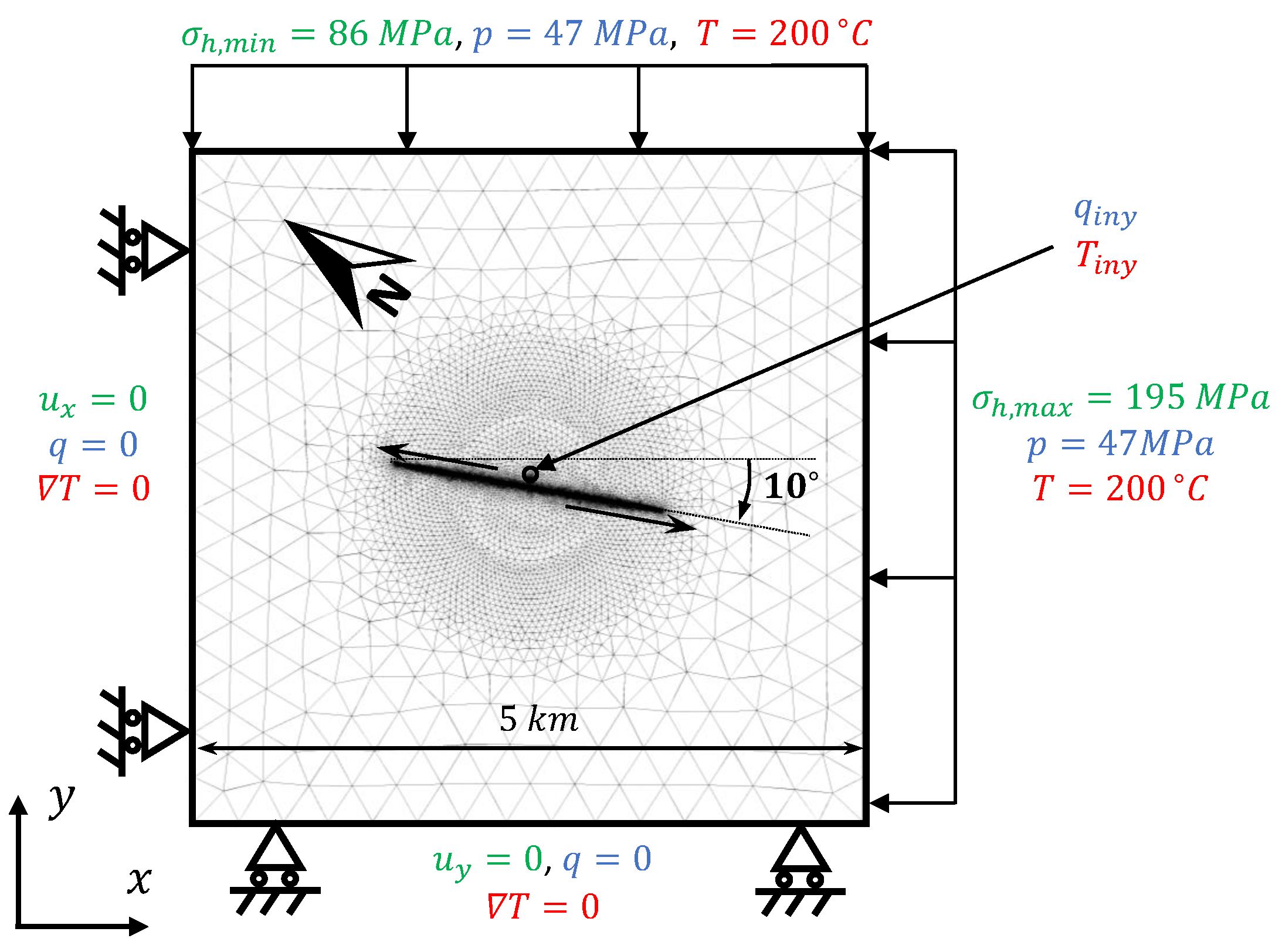
The model is a horizontal section of the reservoir, with the pressure, stress and temperature boundary conditions included in Figure 1. The 2D model domain is a square of 5 km side, with a strike-slip fault of 2000 m length deviated 10${}^{\circ }$ from the x-axis. The direction of the x-axis corresponds to the maximum principal stress ${\sigma }_x$, and the y-axis corresponds to that of the minimum principal stress ${\sigma }_y$. The fault orientation corresponds to the main direction of seismic events in Basel [16]. The injection well is a 5 m radius circle located 50 m away from the midpoint of the fault.

As boundary conditions, the principal stresses are ${\sigma }_y$ = 86 MPa and ${\sigma }_x$ = 195 MPa, which are imposed along two sides of the domain. We also prescribe the hydrostatic pressure, p = 47 MPa, and the temperature due to the geothermal gradient, T = 200 °C, along the same two boundaries. These conditions are consistent with on-site data and measures registered in [15,16]. We restrain the displacement in the normal direction ($\mathbf{u}·\mathbf{n}=0$) and impede both hydraulic and thermal flow ($q=\nabla p=0$, $\nabla T=0$) along the opposite boundaries. At the injection well, we impose a flow velocity $q_{iny}/\left(2\pi rh\right)$, being $q_{iny}$ the injected flow rate, r the radius of the well, and h = 380 m the height of its uncoated part. The flow rate changes according to the injection protocols described in Figure 2a, except for the simulations of Section 3.4 with constant injection and production rates. The temperature at the injection well, $T_{iny}$, is constant with time, but the value depends on the simulation.

We summarize model parameters in

Table 1. Summary of Basel EGS reservoir model parameters, taken from [6].

Parameter	Value	Unit	Description
E	20	GPa	Young modulus of the rock
$\nu$	0.25	–	Poisson ratio of the rock
$\rho$	2700	kg/m${}^3$	Rock density
${\sigma }_y$	86	MPa	Maximum principal stress
${\sigma }_x$	195	MPa	Minimum principal stress
${\rho }_f$	1000	kg/m${}^3$	Fluid density
${\eta }_f$	0.00024	Pa·s	Fluid viscosity
${\chi }_f$	4 × 10${}^{-10}$	Pa${}^{-1}$	Fluid compressibility
k	10${}^{-15}$	m${}^2$	Porous matrix permeability
$\varphi$	0.1	–	Porosity
${\kappa }_s$	2.4	W/(m·K)	Solid thermal conductivity
${\kappa }_f$	0.6	W/(m·K)	Fluid thermal conductivity
$c_s$	800	J/(kg·K)	Solid heat capacity
$c_f$	4200	J/(kg·K)	Fluid heat capacity
T${}_0$	473.15	K	Natural temperature
${\alpha }_B$	1	–	Biot coefficient
${\alpha }_T$	8 × 10${}^{-6}$	K${}^{-1}$	Thermal expansion coefficient
${\mu }_0$	0.55	–	Friction coefficient
a	0.005	–	Direct effect parameter
b	0.03	–	Friction evolution parameter
$D_c$	0.0007	m	Characteristic slip distance
$V^{*}$	10${}^{-9}$	m/s	Reference slip velocity
$\alpha$	0.2	–	Linker–Dieterich stressing rate coefficient

. Mechanical parameters are usual values for crystalline granitic rock massifs. The Young modulus is E = 20 GPa, the Poisson ratio $\nu$ = 0.25, and the density of the solid skeleton is $\rho$ = 2700 kg/m${}^3$. Fluid parameters are ${\rho }_f$ = 1000 kg/m${}^3$, ${\eta }_f$ = 0.00024 Pa·s and ${\chi }_f$ = 4 × 10${}^{-10}$ Pa${}^{-1}$, which are, respectively, the density, dynamic viscosity and compressibility of water at the reservoir depth. The density and compressibility, even if affected by temperature and pressure, vary slightly compared to the viscosity, which is much lower than the value at ambient conditions (${\eta }_f$ = 0.001 Pa·s) given the pressure and temperature conditions at the depths studied [88].

The porous matrix permeability and porosity are k = 10${}^{-15}$ m${}^2$ and $\varphi$ = 0.1, based on the characteristics of the rock mass [16,62], although the measurements of these parameters around the injection well can be quite different depending on several studies and interpretations [60]. The solid thermal conductivity is ${\kappa }_s$ = 2.4 W/(m·K), the fluid thermal conductivity is ${\kappa }_f$ = 0.6 W/(m·K), the solid heat capacity is $c_s$ = 800 J/(kg·K) and the fluid heat capacity is $c_f$ = 4200 J/(kg·K), according to the materials and parameters collected in [89]. The Biot coefficient ${\alpha }_B$ = 1 couples fluid flow and mechanical problems, and the thermal expansion coefficient ${\alpha }_T$ = 8 · 10${}^{-6}$ couples thermal and mechanical physics.

We choose frictional parameters within feasible ranges to simulate the seismic rupture propagation and fault reactivation in accordance with on-site registered time scales. The Linker–Dieterich parameter is $\alpha$ = 0.2, the initial friction coefficient is ${\mu }_0$ = 0.55, the direct effect parameter is a = 0.005, the friction evolution parameter is b = 0.03, the characteristic slip distance is $D_c$ = 0.0007 m, and the reference slip velocity is $V^{*}$ = 10${}^{-9}$ m/s [6,63].

We solve Equations (1)–(14) in a monolithically coupled fashion and the rate-and-state aging law (16) and (17) along the fault [6,63,70,71], using the finite element software COMSOL Multiphysics. The frictional contact is modeled using an Augmented Lagrangian formulation [90], and transport along the fault is solved introducing the weak form of Equations (8) and (13) to the overall variational formulation of the Darcy flow and heat transport problems. We discretize the domain in triangular elements with quadratic interpolation for displacements and linear for pore pressure and temperature.

3. Results

3.1. Fault Reactivation and Injection Design

We simulate the thermo-geomechanical response of the Basel EGS reservoir during the hydraulic stimulation phase up to the fault reactivation, and we study the frictional response of the fault under several injection protocols. We assume that the water temperature in the head of the injection well is 20 °C. We define the point on the fault where the slip starts as the control point, and we plot the change in several variables with time.

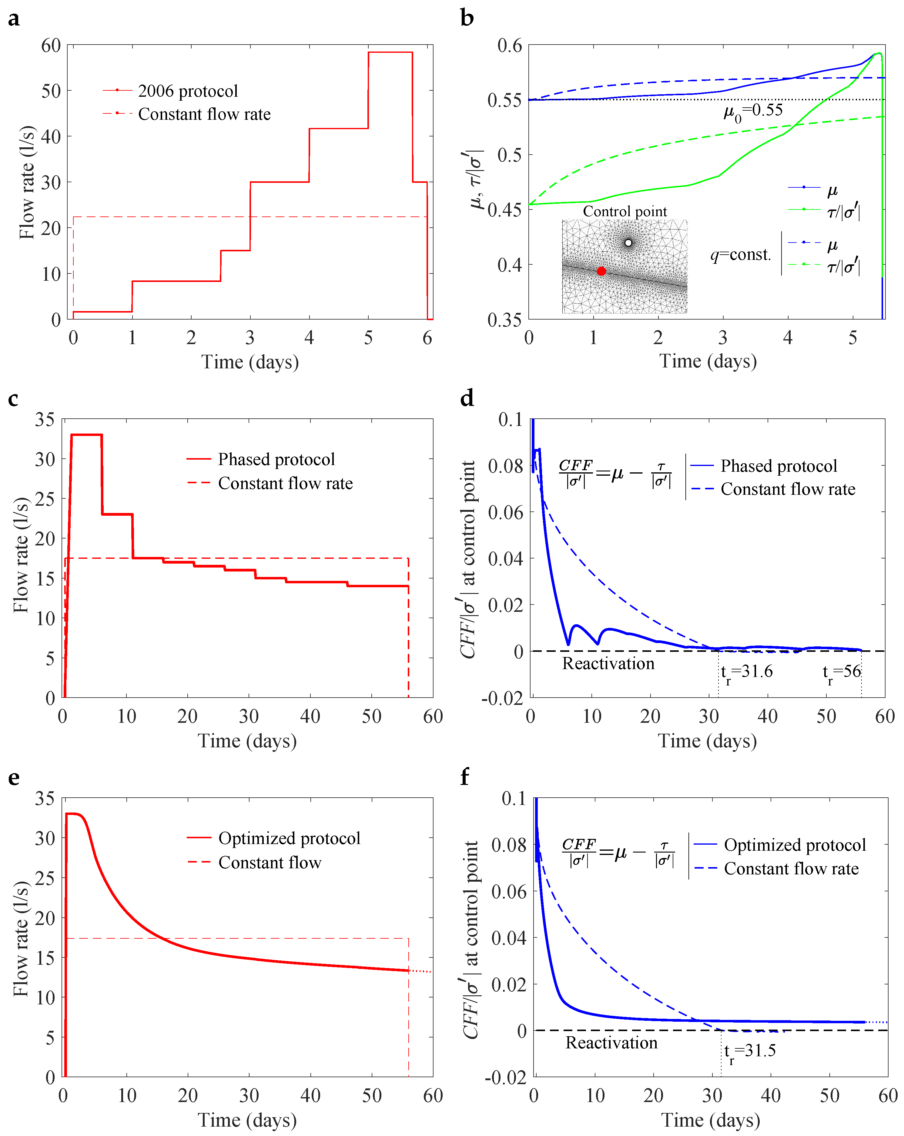
The hydraulic stimulation phase of the Basel EGS reservoir required the injection of 11,600 m${}^3$ of water for 6 days, according to the injection protocol depicted in Figure 2a [16]. If the water volume had been injected at a constant flow rate for 6 days, the injection flow rate would have been 22.4 l/s. We also plot this simplified injection protocol in Figure 2a. We simulate these two injection protocols and plot the results of the friction variables on the control point of the fault in Figure 2b. The friction coefficient $\mu$ (blue line) and the ratio $\tau /|{\sigma }^{\prime }|$ (green line) show that the model predicts the fault reactivation at 5.5 days, as our previous 3D model predicted [6]. The injection at a constant flow rate (dashed line) does not reactivate the fault instead for the first 6 days.

Figure 3 shows the changes in pressure and temperature around the injection well with the 2006 injection protocol. These results highlight that the changes in temperature induced by the injection of cold water are irrelevant in the short term, so the injection has to last several years to generate thermal effects on the reservoir.

We conclude that the conducted hydraulic stimulation with 11,600 m${}^3$ of water may have been performed with our optimized protocol without relevant seismic risk. Nevertheless, the hydraulic stimulation in EGS geothermal power plants requires about 7570 m${}^3$ of water per MW [91], which in the case of the 23 MW Basel power plant, the total water volume would have been 174,110 m${}^3$. This estimation of the required water volume for the hydraulic stimulation shows that the operation was interrupted at an early stage.

The question is how to inject that volume without triggering a high seismic event. On the one hand, Figure 2b shows that although the fault would not have reactivated for the first 6 days with a constant injection flow rate, there is a small resistance margin that indicates the fault would have reactivated soon if the injection had continued. However, if the flow rate had decreased, the fault reactivation would have been delayed. On the other hand, the injection phase would have been shortened if the injection rate had been increased, but the seismic risk would have also increased due to the additional increase in pore pressure. Therefore, Figure 2a,b show that it is necessary to explore other injection strategies to avoid the eventual fault reactivation. In such a way, it is important to take advantage of the contact frictional properties. Fault reactivation and frictional behavior can be affected by the rate of change in pore pressure: an increase of pressure, due to fluid injection, can lead an increase in friction coefficient and then a delayed weakening of the fault, while a sharp pressure decrease associated with fluid production can promote to a delayed strengthening [63].

We design a phased injection protocol that fully exploits that frictional properties on the fault, with an early maximum flow rate followed by an extended decline. The protocol is divided into phases of 5 days, and the injected flow rate is constant in each phase. Figure 2c shows the series of flow rate steps, that is 33, 23, 17.5, 17, 16.5, 16, 15, 14.5, 14.5, 14 and 14 l/s. Figure 2d represents the evolution of the dimensionless Coulomb failure function, $CFF/|{\sigma }^{\prime }|$, on the control point on the fault. In this work, negative values of $CFF$ mean fault reactivation, while positive $CFF$ implies that fault are still at rest. The results show that the phased injection protocol reduces the frictional strength on the fault in each step without reaching the reactivation for up to 56 days. If the same volume of water had been injected at a constant flow rate (17.4 l/s), the reactivation would have occurred earlier, after 31.6 days of injection. Our phased injection protocol would let us inject about 84,000 m${}^3$ of water, which is a volume higher than the real injected volume.

We propose an injection flow law for the stimulation protocol that automatically controls the flow rate according to how close the fault is to the reactivation. We establish a flow law that depends on the Coulomb function, $CFF$. Thus, if the fault approaches the reactivation and the CFF is close to 0, the flow rate will decrease to avoid fault slip. The proposed law is:

$$q_{iny}=q_0\left(1-exp\left(-\frac{CF{F}_{min}\left(t\right)}{CF{F}_{min,0}}{R}_q\right)\right),$$

(20)

where $q_0$ is the initial flow rate, $R_q$ is a fitting parameter, $CF{F}_{min}\left(t\right)$ is the minimum value of the Coulomb failure function along the fault at each time step and $CF{F}_{min,0}$ is the minimum value of the Coulomb failure function along the fault at t = 0. Figure 2e shows the injection flow rate for two injection protocols: (1) our optimized law, for $q_0$ = 33 l/s and $R_q$ = 15, and (2) an injection protocol with a constant flow rate and equal injected volume as the optimized protocol. The optimized protocol injects initially water at a constant flow rate and after a few days, the rate decreases exponentially. Figure 2f shows the change in the dimensionless Coulomb failure function with time on the control point of the fault. Our optimized protocol avoids the reactivation after 56 days, whereas the protocol with a constant flow rate generates the reactivation of the fault after 31.5 days of injection.

In Figure 2c,e the injection protocols have similar durations and injection volumes. The phased protocol and the optimized protocol have a similar change in the $CFF$. Nevertheless, the former protocol produces the reactivation after 56 days of injection, while the latter protocol avoids the reactivation and maintains a safety margin ($CFF>0$ in Figure 2f). In both cases, the injection at a constant flow rate produces the reactivation of the fault at a similar time.

These results highlight that injection protocols may be designed to avoid or delay fault reactivation. Our optimized injection law may minimize seismic risks in terms of fault reactivation for fixed frictional parameters. Nevertheless, there may be some uncertainty regarding the poromechanical parameters of the model, and some changes in frictional parameters could lead to quantitatively different results. In such a sense, rate-and-state parameters b and $\alpha$ would be especially sensitive, since they control the fault delayed weakening, as already stated in our previous work [63]. Therefore, sensitivity analysis of frictional parameters should be performed in future studies for each injection protocol.

3.2. Seismic Rupture and Earthquake Magnitude

The hydraulic stimulation may have some undesirable effects, such the fault reactivation that may trigger an earthquake. The hydro-shearing technique enhances the fault permeability with water injections at high pressure, reactivating the fault and inducing the slip [92]. The process may trigger an earthquake if the slip on the fault is coseismic. Our numerical model can reproduce the fault reactivation, the permeability enhancement on the fault, as well as the fault rupture. Therefore, we can determine if the fault reactivation is aseismic, or on the contrary, coseismic with our model.

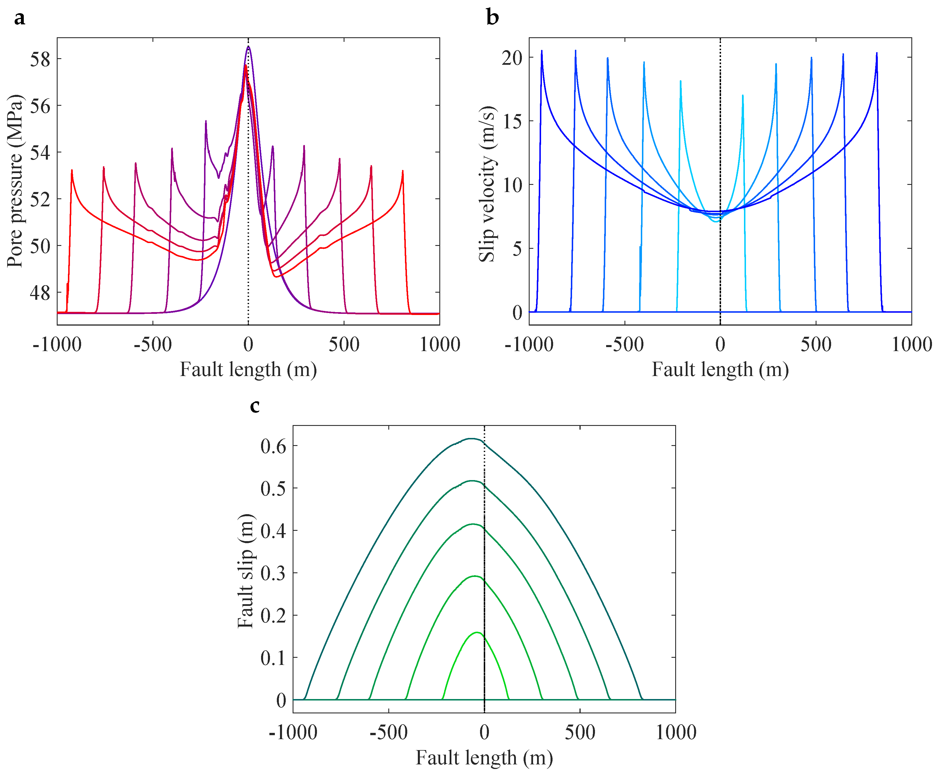
Figure 4a,b include the undrained pressure and slip velocity fronts at several time steps during a rupture for the 2006-Basel injection protocol included in Figure 2a. We observe that for the Basel reservoir conditions, the model predicts an almost symmetrical propagation of the rupture. Both the undrained pressure and the slip velocity fronts propagate at similar speeds in both directions of the fault. Figure 4c shows the slip of the fault at the same time steps.

We estimate the earthquake magnitude with Equations (18) and (19). Previous studies point out that the approximate thickness of the zone of hypocenters is 500 m [16,93], which leads to a moment magnitude $M_w$ = 3.8. This magnitude is slightly higher than the real local value registered in 2006, although our result may be refined by calibrating the friction parameters.

We estimate the earthquake magnitude under our two optimized injection protocols depicted in Figure 2c. The magnitude is slightly higher than the previous one, 3.9 in the case of the phased protocol and 3.85 in the case of injection at a constant flow rate. These results highlight an important aspect: the delay in the reactivation with the optimized injection protocols leads to larger seismic events when the fault reactivates. Therefore, for the same water injection volume, the delay in the peak flow rate may minimize the earthquake magnitude. These results agree with a previous case study [94] which foresees larger seismic events for early peak flows, although deeper studies regarding this phenomenon should be conducted.

3.3. Permeability Enhancement

The hydraulic stimulation is mainly aimed to increase the permeability of the fracture network and achieve higher energy efficiency. Here, we deal with the permeability enhancement of the fracture network in the Basel reservoir. We use our model as a conceptual example and assume that the permeability of the entire fractured area around the fault can be simulated with the fault permeability.

We solve Equations (8)–(12) for fluid flow and Equations (13) and (14) for heat transport along the fault. We consider that the fault permeability changes with fault slip so that both seismic and co-seismic slip produce an increase in permeability, both longitudinally and across the fault [95]. This allows us to reproduce the permeability stimulation in the fractures with a mechanism similar to hydro-shearing. We review the literature to quantify the increase in permeability due to hydro-shearing. Experiments performed on samples with a single fracture indicate that the permeability of a hydraulically stimulated contact increases by an order of magnitude due to slip [96,97], while hydraulic fracture experiments indicate that this rise can reach three orders of magnitude [98]. Therefore, we assume that permeability increases one or two orders of magnitude with fault slip.

We perform one simulation as a conceptual example. We adopt the rock and fluid properties listed in Table 1 and introduce the following fault permeability law that reads:

$$k_{fr}={10}^{(-10-(-10+12)exp(-\left|\delta \right|/{\delta }_0\left)\right)},$$

(21)

where $\delta$ is the relative slip between the fault walls, ${\delta }_0$ is a fitting parameter that acts as a threshold displacement and $k_{fr}$ is the permeability of the fault. Thus, the permeability in the longitudinal direction along the fault may vary between ${10}^{-10}$ and ${10}^{-12}$ m${}^2$. The transversal fault permeability is governed by a similar expression:

$$k_{T,fr}={10}^{(-10-(-10+14)exp(-\left|\delta \right|/{\delta }_0\left)\right)},$$

(22)

where we take ${\delta }_0$ = 0.6 m. The upper permeability limit, 10${}^{-10}$ m${}^2$, is high enough so the flow along the fault is relevant, and the lower limit, 10${}^{-12}$ m${}^2$, makes the fault permeability barely influences the pressure propagation before the sliding. We consider that the thermal parameters on the fault and the host rock are the same; thus, heat transport by advection dominates over diffusion.

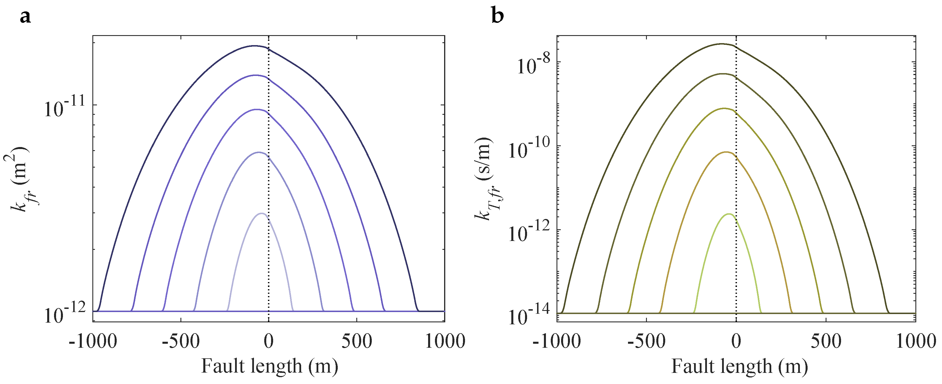
Figure 5 shows the increases in both longitudinal and transverse fault permeability. The permeability enhancements do not substantially affect seismicity, since the rupture propagation and the eventual earthquake magnitude have similar values to the simulation without permeability enhancement. Our results are sensitive to the displacement threshold, ${\delta }_0$, the permeability thresholds, and the aperture $d_{fr}$; therefore, some combination of values may substantially alter the rupture and the eventual earthquake magnitude. Our fault permeability law is a feasible way to reproduce the permeability enhancement due to the hydraulic stimulation.

3.4. Long-Term Operation and Thermal Decline

Numerical models are useful tools to analyze the long-term behavior of geothermal reservoirs in terms of produced energy, efficiency, and thermal decline. Models may be also useful tools to assess hypothetical operation strategies in the long term. We run long-term simulations to analyze the thermal behavior of our case study during its lifetime. We assume fractures are hydraulic stimulated, and we adopt the fault permeability values reported in the previous section. We consider that the lifetime of the Basel geothermal reservoir would have been 30 years [3,91].

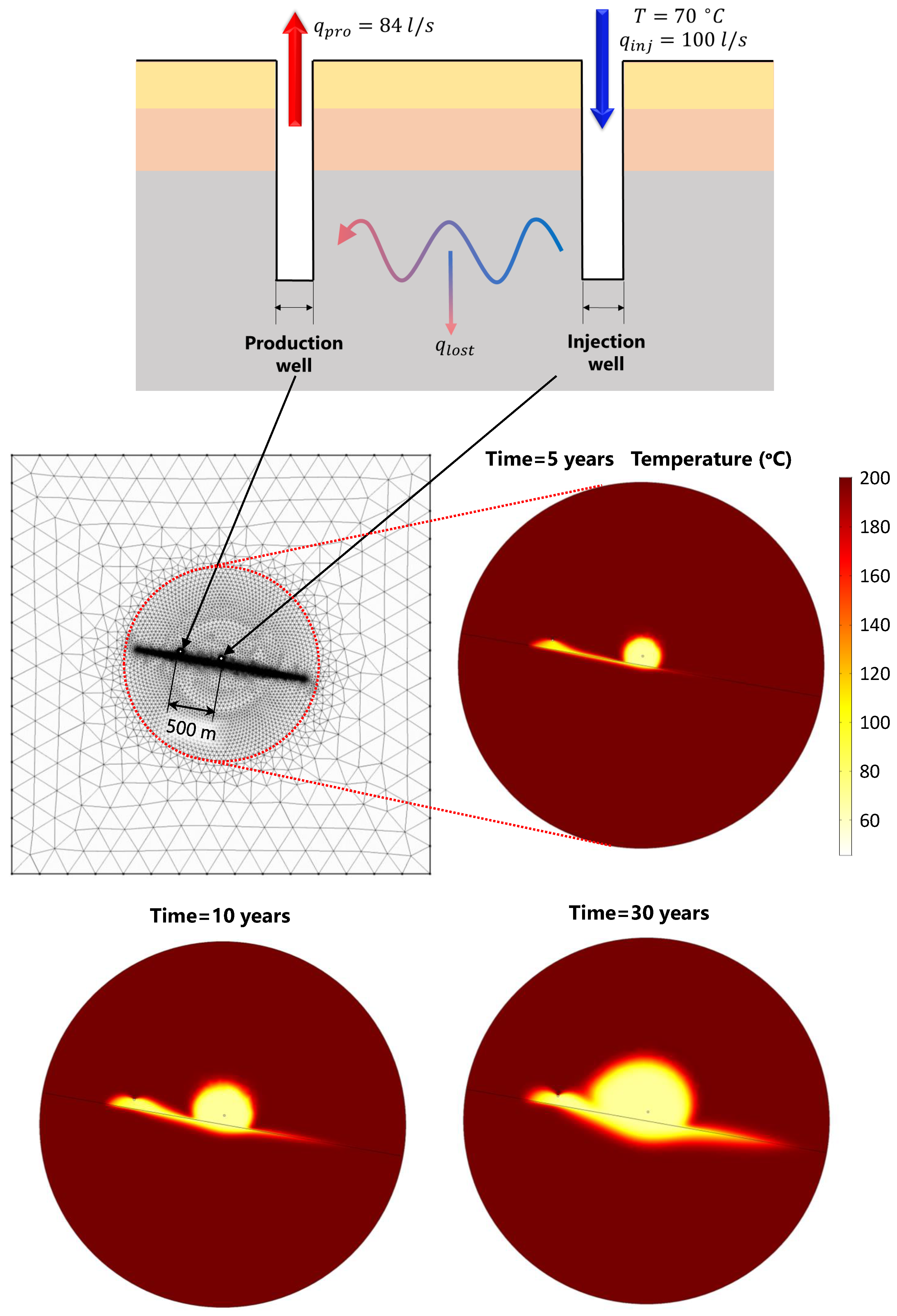
The injected and extracted flow rate is compulsory data for our numerical simulations. The thermal power given by a flow rate is $P={\rho }_f{c}_{f}q\Delta T$, where ${\rho }_f$ is the fluid density, $c_f$ is the specific heat of the fluid, q is the flow rate, and $\Delta T$ is the temperature difference of the fluid in the head of the injection and production wells. For a 23 MW thermal power and a temperature difference of $\Delta T$ = 130 °C, with ${\rho }_f$ = 1000 kg/m${}^3$ and $c_f$ = 4200 J/(kg K), the flow rate is q = 42.1 l/s. Assuming that the global efficiency of the system is 50% since hot water would have been fundamentally employed for non-electrical use in Basel [3], the produced water flow rate would have to be 84.2 l/s.

We have to take into account the water loss that takes place in the reservoir. According to [91], water losses throughout the lifetime of an EGS plant are about 530,000 m${}^3$ per MW of power. For a 23 MW power plant and a lifetime of 30 years, the annual water loss is 406,000 m${}^3$. We add this extra annual water volume to the injected flow rate and the total injected flow rate is approximately 100 l/s.

We simulate the thermal behavior for 30 years of operation with these injections and production flow rates, and the thermo-mechanical properties are listed in Table 1. We assume that both the injection and production wells are on the same side of the fault and the distance between both wells is 500 m. Our simulations show that the fault is reactivated several times; however, the magnitude of these seismic events is quite low compared to the events triggered during the hydraulic stimulation.

Figure 6 depicts the temperature field at 5, 10, and 30 years. We observe that heat is mainly transported by advection in the vicinity of the fault once the temperature drop around the well reaches it. Subsequently, the cooling reaches the extraction well and extends to larger areas around the injection well.

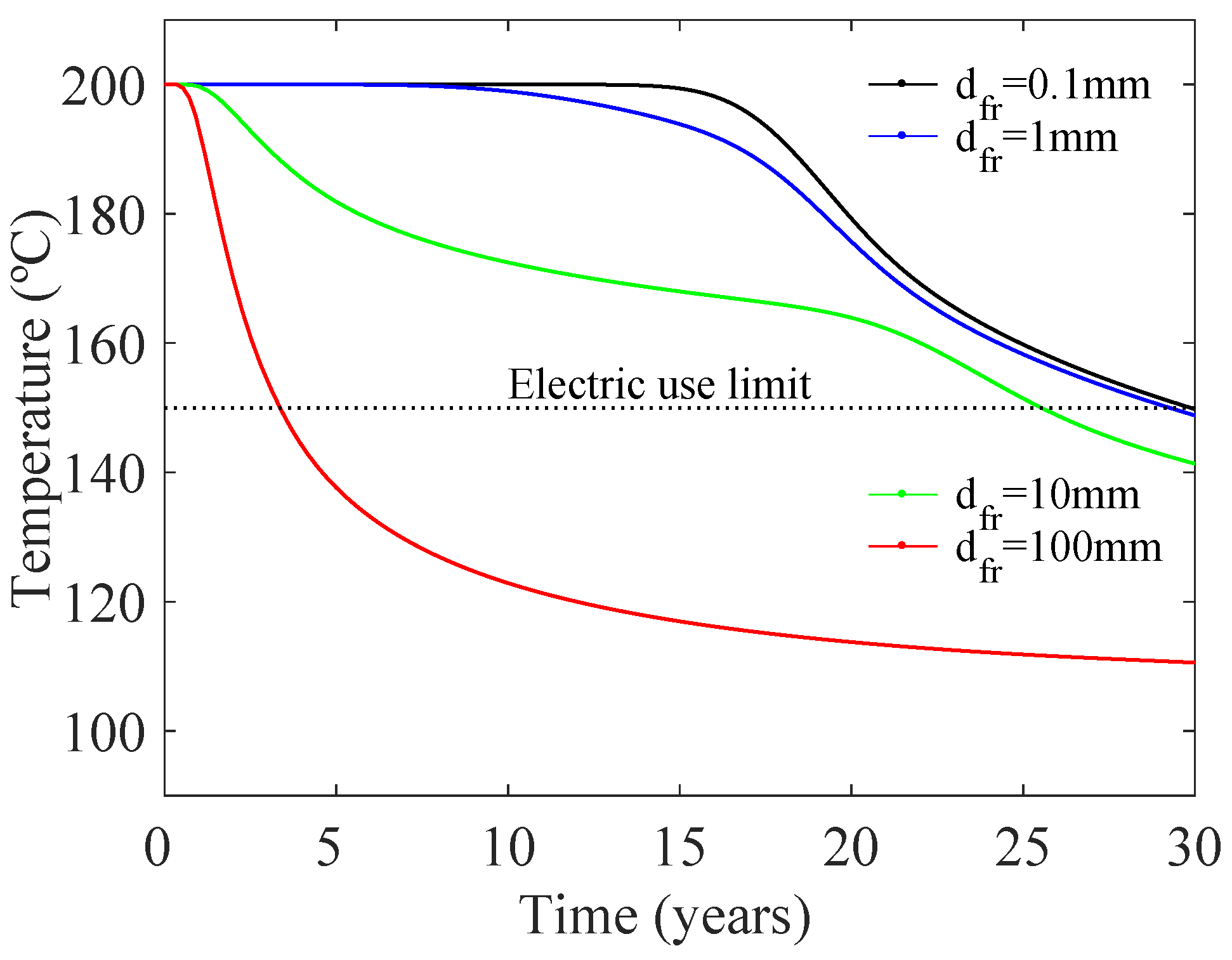
These results show that the fault permeability directly influences the long-term thermal decline: as the permeability increases, the thermal decline is faster [64,65], as represented in Figure 7. Recent research works relate heat production with the fracture network topology and they reach similar conclusions to our work [66,67]. Our results support the conception that geothermal reservoirs may be economically feasible for two or three decades. Although reservoirs would naturally recover heat by diffusion, several centuries are required since heat transport by diffusion is much slower than by advection.

These results are heavily dependent on several parameters and are open to interpretations and assumptions: the fault zone width, the permeability thresholds assigned to the fault, or the relative position of the injection and production wells. The role of rock thermal contraction on fault aperture could also be considered as another factor that varies fault permeability in the long term [99,100,101]. Changes in all these assumptions would result in new results, highlighting that our numerical model is a useful tool to assess the long-term operation of geothermal reservoirs.

In our simulations, the flow rates on the injection and production wells are imposed as boundary conditions, so the pressures required to inject and produce the rates are conditioned by the host rock permeability and the fluid viscosity. Then, if the host rock has low permeability, the pressure required to inject the water at the desired flow rate may be impossible to achieve with the current technology. This would lead to considering the permeability enhancement with hydraulic stimulation. However, the increase in the host rock permeability may increase the seismic risk and lead to the early thermal decline of the rock mass. Therefore, the hydraulic stimulation operations should be designed taking into account the balance between seismic risk and early thermal decline.

4. Conclusions

In this work, we proposed a numerical model to simulate the thermo-hydro-mechanical behavior of Enhanced Geothermal Systems (EGS) reservoirs and simulate induced earthquakes driven by fluid injection. We focused on the hydraulic stimulation of the Basel EGS reservoir.

Our numerical simulations show that it is possible to anticipate the largest induced seismic event that took place in Basel in 2006. We analyze the fault reactivation, the rupture propagation, and estimate the magnitude of the eventual earthquake. Our results are quite consistent with the existing records.

Moreover, we use our model to study several hydraulic stimulation scenarios and propose EGS operation protocols to minimize seismic risks. We explored the optimization of the injection protocols to avoid fault reactivation, for fixed frictional parameters and a certain water volume to inject.

In the long-term, we observe that several years are necessary to induce appreciable thermal changes in the reservoir. These changes could lead to a thermal decline of the reservoir, which will greatly depends on the permeability of the fractures in the host rock and the enhancement achieved with hydraulic stimulation.

Our model can be a useful tool to achieve a balance between hydraulic stimulation, induced seismicity, and energy production in geothermal reservoirs. Our results will contribute to assessing operation protocols, control seismic risks, and may help practitioners and stakeholders to make decisions regarding this disruptive technology and reduce the social opposition to EGS projects.

References

- Colglazier, W. Sustainable development agenda: 2030. Science 2015, 349, 1048–1050. [Google Scholar] [CrossRef] [PubMed]
- Mahbaz, S.; Dehghani-Sanij, A.; Dusseault, M.; Nathwani, J. Enhanced and integrated geothermal systems for sustainable development of Canada’s northern communities. Sustain. Energy Technol. Assess. 2020, 37, 100565. [Google Scholar] [CrossRef]
- MIT Energy Initiative. The Future of Geothermal Energy: Impact of Enhanced Geothermal Systems (EGS) on the United States in the 21st Century; Massachusetts Institute of Technology: Cambridge, MA, USA, 2006. [Google Scholar]
- Kinney, C.; Dehghani-Sanij, A.; Mahbaz, S.; Dusseault, M.; Nathwani, J.; Fraser, R. Geothermal Energy for Sustainable Food Production in Canada’s Remote Northern Communities. Energies 2019, 12, 4058. [Google Scholar] [CrossRef] [Green Version]
- Soltani, M.; Moradi-Kashkooli, F.; Dehghani-Sanij, A.; Nokhosteen, A.; Ahmadi-Joughi, A.; Gharali, K.; Mahbaz, S.; Dusseault, M. A comprehensive review of geothermal energy evolution and development. Int. J. Green Energy 2019, 16, 971–1009. [Google Scholar] [CrossRef]
- Andrés, S.; Santillán, D.; Mosquera, J.; Cueto-Felgueroso, L. Thermo-Poroelastic Analysis of Induced Seismicity at the Basel Enhanced Geothermal System. Sustainability 2019, 11, 6904. [Google Scholar] [CrossRef] [Green Version]
- Santillan, D.; Mosquera, J.; Cueto-Felgueroso, L. Fluid-driven fracture propagation in heterogeneous media: Probability distributions of fracture trajectories. Phys. Rev. E 2017, 96, 053002. [Google Scholar] [CrossRef]
- Santillán, D.; Juanes, R.; Cueto-Felgueroso, L. Phase field model of hydraulic fracturing in poroelastic media: Fracture propagation, arrest, and branching under fluid injection and extraction. J. Geophys. Res. Solid Earth 2018, 123, 2127–2155. [Google Scholar] [CrossRef] [Green Version]
- Rinaldi, A.; Rutqvist, J.; Sonnenthal, E.; Cladouhos, T. Coupled THM Modeling of Hydroshearing Stimulation in Tight Fractured Volcanic Rock. Transp. Porous Med. 2014, 108, 131–150. [Google Scholar] [CrossRef] [Green Version]
- Rinaldi, A.; Rutqvist, J. Joint opening or hydroshearing? Analyzing a fracture zone stimulation at Fenton Hill. Geothermics 2019, 77, 83–98. [Google Scholar] [CrossRef] [Green Version]
- Giardini, D. Geothermal quake risks must be faced. Nature 2009, 462, 848–849. [Google Scholar] [CrossRef]
- Schultz, R.; Skoumal, R.; Brudzinski, M.; Eaton, D.; Baptie, B.; Ellsworth, W. Hydraulic Fracturing-Induced Seismicity. Rev. Geophys. 2020, 58, e2019RG000695. [Google Scholar] [CrossRef]
- Parker, R. The Rosemanowes HDR project 1983–1991. Geothermics 1999, 28, 603–615. [Google Scholar] [CrossRef]
- Pine, R.; Batchelor, A. Downward migration of shearing in jointed rock during hydraulic injections. Int. J. Rock. Mech. Min. Sci. Geomech. Abstr. 1984, 21, 249–263. [Google Scholar] [CrossRef]
- Häring, M.; Hopkirk, R. The Swiss Deep Heat Mining Project-The Basel Exploration Drilling. GHC Bull. 2002, 23, 31–33. [Google Scholar]
- Häring, M.; Schanz, U.; Ladner, F.; Dyer, B. Characterisation of the Basel 1 enhanced geothermal system. Geothermics 2008, 37, 469–495. [Google Scholar] [CrossRef]
- Baisch, S.; Vörös, R.; Weidler, R.; Wyborn, D. Investigation of Fault Mechanisms during Geothermal Reservoir Stimulation Experiments in the Cooper Basin, Australia. Bull. Seismol. Soc. Am. 2009, 99, 148–158. [Google Scholar] [CrossRef]
- Ellsworth, W.; Giardini, D.; Townend, J.; Ge, S.; Shimamoto, T. Triggering of the Pohang, Korea, Earthquake (Mw 5.5) by Enhanced Geothermal System Stimulation. Seismol. Res. Lett. 2019, 90, 1844–1858. [Google Scholar] [CrossRef]
- Chang, K.; Yoon, H.; Kim, Y.; Lee, M. Operational and geological controls of coupled poroelastic stressing and pore-pressure accumulation along faults: Induced earthquakes in Pohang, South Korea. Sci. Rep. 2020, 10, 2073. [Google Scholar] [CrossRef] [Green Version]
- Ziagos, J.; Phillips, B.; Boyd, L.; Jelacic, A.; Stillman, G.; Hass, E. A Technology Roadmap for Strategic Development of Enhanced Geothermal Systems. In Proceedings of the 38th Workshop on Geothermal Reservoir Engineering, Stanford, CA, USA, 11–13 February 2013. [Google Scholar]
- Minetto, R.; Montanari, D.; Planès, T.; Bonini, M.; Ventisette, C.; Antunes, V.; Lupi, M. Tectonic and Anthropogenic Microseismic Activity While Drilling Toward Supercritical Conditions in the Larderello-Travale Geothermal Field, Italy. J. Geophys. Res. Solid Earth 2020, 125, e2019JB018618. [Google Scholar] [CrossRef]
- Bagagli, M.; Kissling, E.; Piccinini, D.; Saccorotti, G. Local earthquake tomography of the Larderello-Travale geothermal field. Geothermics 2020, 83, 101731. [Google Scholar] [CrossRef]
- Rutqvist, J.; Jeanne, P.; Dobson, P.; Garcia, J.; Hartline, C.; Hutchings, L.; Singh, A.; Vasco, D.; Walters, M. The Northwest Geysers EGS Demonstration Project, California—Part2: Modeling and interpretation. Geothermics 2016, 63, 120–138. [Google Scholar] [CrossRef]
- Garcia, J.; Hartline, C.; Walters, M.; Wright, M.; Rutqvist, J.; Dobson, P.; Jeanne, P. The Northwest Geysers EGS Demonstration Project, California—Part 1: Characterization and reservoir response to injection. Geothermics 2016, 63, 97–119. [Google Scholar] [CrossRef] [Green Version]
- Kim, K.; Ree, J.; Kim, Y.; Kim, S.; Kang, S.; Seo, W. Assessing whether the 2017 Mw 5.4 Pohang earthquake in South Korea was an induced event. Science 2018, 360, 1007–1009. [Google Scholar] [CrossRef] [PubMed] [Green Version]
- Grigoli, F.; Cesca, S.; Rinaldi, A.; Manconi, A.; López-Comino, J.; Clinton, J.; Westaway, R.; Cauzzi, C.; Dahm, T.; Wiemer, S. The November 2017 Mw 5.5 Pohang earthquake: A possible case of induced seismicity in South Korea. Science 2018, 360, 1003–1006. [Google Scholar] [CrossRef] [Green Version]
- Hubbert, M.; Rubey, W. Role of fluid pressure in mechanics of overthrust faulting I. Mechanics of fluid-filled porous solids and its application to overthrust faulting. Geol. Soc. Am. Bull. 1959, 70, 115–166. [Google Scholar]
- Pampillón, P.; Santillán, D.; Mosquera, J.; Cueto-Felgueroso, L. Geomechanical Constraints on Hydro-Seismicity: Tidal Forcing and Reservoir Operation. Water 2020, 12, 2724. [Google Scholar] [CrossRef]
- Pampillón, P.; Santillán, D.; Mosquera, J.; Cueto-Felgueroso, L. Dynamic and Quasi-Dynamic Modeling of Injection-Induced Earthquakes in Poroelastic Media. J. Geophys. Res. Solid Earth 2018, 123, 5730–5759. [Google Scholar] [CrossRef]
- National Research Council. Induced Seismicity Potential in Energy Technologies; The National Academies Press: Washington, DC, USA, 2013. [Google Scholar]
- Ellsworth, W. Injection-Induced Earthquakes. Science 2013, 341, 1225942. [Google Scholar] [CrossRef]
- Brodsky, E.; Lajoie, L. Anthropogenic Seismicity Rates and Operational Parameters at the Salton Sea Geothermal Field. Science 2013, 341, 543–546. [Google Scholar] [CrossRef]
- Buijze, L.; van Bijsterveldt, L.; Cremer, H.; Paap, B.; Veldkamp, H.; Wassing, B.; van Wees, J.; van Yperen, J.; ter Heege, J.; Jaarsma, B. Review of induced seismicity in geothermal systems worldwide and implications for geothermal systems in the Netherlands. Neth. J. Geosci. 2019, 98, E13. [Google Scholar] [CrossRef] [Green Version]
- Horton, S. Disposal of hydrofracking waste fluid by injection into subsurface aquifers triggers earthquake swarm in central Arkansas with potential for damaging earthquake. Seismol. Res. Lett. 2012, 83, 250–260. [Google Scholar] [CrossRef] [Green Version]
- Juanes, R.; Hager, B.; Herzog, H. No geologic evidence that seismicity causes fault leakage that would render large-scale carbon capture and storage unsuccessful. Proc. Natl. Acad. Sci. USA 2012, 109, E3623. [Google Scholar] [CrossRef] [PubMed]
- Vilarrasa, V.; Carrera, J. Geologic carbon storage is unlikely to trigger large earthquakes and reactivate faults through which CO2 could leak. Proc. Natl. Acad. Sci. USA 2015, 112, 5938–5943. [Google Scholar] [CrossRef] [PubMed] [Green Version]
- White, J.; Foxall, W. Assessing induced seismicity risk at CO2 storage projects: Recent progress and remaining challenges. Int. J. Greenh. Gas Control 2016, 49, 413–424. [Google Scholar] [CrossRef] [Green Version]
- Vilarrasa, V.; De Simone, S.; Carrera, J.; Villaseñor, A. Unraveling the causes of the seismicity induced by underground gas storage at Castor, Spain. Geophys. Res. Lett. 2021, 48, e2020GL092038. [Google Scholar] [CrossRef]
- Weingarten, M.; Ge, S.; Godt, J.; Bekins, B.; Rubinstein, J. High-rate injection is associated with the increase in U.S. mid-continent seismicity. Science 2015, 348, 1336–1340. [Google Scholar] [CrossRef] [PubMed] [Green Version]
- Shirzaei, M.; Ellsworth, W.; Tiampo, K.; González, P.; Manga, M. Surface uplift and time-dependent seismic hazard due to fluid injection in eastern Texas. Science 2016, 353, 1416–1419. [Google Scholar] [CrossRef] [Green Version]
- McComas, K.; Lu, H.; Keranen, K.; Furtney, M.; Song, H. Public perceptions and acceptance of induced earthquakes related to energy development. Energy Policy 2016, 99, 27–32. [Google Scholar] [CrossRef]
- Mignan, A.; Karvounis, D.; Broccardo, M.; Wiemer, S.; Giardini, D. Including seismic risk mitigation measures into the Levelized Cost of Electricity in enhanced geothermal systems for optimal siting. Appl. Energy 2019, 238, 831–850. [Google Scholar] [CrossRef]
- Lee, K.; Ellsworth, W.; Giardini, D.; Townend, J.; Ge, S.; Shimamoto, T.; Yeo, I.; Kang, T.; Rhie, J.; Sheen, D.; et al. Managing injection-induced seismic risks. Science 2019, 364, 730–732. [Google Scholar] [CrossRef]
- McGarr, A. Maximum magnitude earthquakes induced by fluid injection. J. Geophys. Res. Solid Earth 2014, 119, 1008–1019. [Google Scholar] [CrossRef]
- Scholz, C. The Mechanics of Earthquakes and Faulting; Cambridge University Press: Cambridge, UK, 2002. [Google Scholar]
- Charlety, J.; Cuenot, N.; Dorbath, L.; Dorbath, C.; Haessler, H.; Frogneux, M. Large earthquakes during hydraulic stimulations at the geothermal site of Soultz-sous-Forêts. Int. J. Rock. Mech. Min. Sci. 2007, 44, 1091–1105. [Google Scholar] [CrossRef]
- Deichmann, N.; Giardini, D. Earthquakes Induced by the Stimulation of an Enhanced Geothermal System below Basel (Switzerland). Seismol. Res. Lett. 2009, 80, 784–798. [Google Scholar] [CrossRef]
- De Simone, S.; Carrera, J.; Vilarrasa, V. Superposition approach to understand triggering mechanisms of post-injection induced seismicity. Geothermics 2017, 70, 85–97. [Google Scholar] [CrossRef]
- Rutqvist, J.; Birkholzer, J.; Tsang, C.F. Coupled reservoir-geomechanical analysis of the potential for tensile and shear failure associated with CO2 injection in multilayered reservoir-caprock systems. Int. J. Rock. Mech. Min. Sci. 2008, 45, 132–143. [Google Scholar] [CrossRef] [Green Version]
- De Simone, S.; Vilarrasa, V.; Carrera, J.; Alcolea, A.; Meier, P. Thermal coupling may control mechanical stability of geothermal reservoirs during cold water injection. Phys. Chem. Earth 2013, 64, 117–126. [Google Scholar] [CrossRef]
- Vilarrasa, V.; Olivella, S.; Carrera, J.; Rutqvist, J. Long term impacts of cold CO2 injection on the caprock integrity. Int. J. Greenh. Gas Control 2014, 24, 1–13. [Google Scholar] [CrossRef]
- Jacquey, A.; Cacace, M.; Blöcher, G.; Watanabe, N.; Huenges, E.; Scheck-Wenderoth, M. Thermo-poroelastic numerical modelling for enhanced geothermal system performance: Case study of the Groß Schönebeck reservoir. Tectonophysics 2016, 684, 119–130. [Google Scholar] [CrossRef]
- Rice, J. Heating and weakening of faults during earthquake slip. J. Geophys. Res. 2006, 111, B05311. [Google Scholar] [CrossRef] [Green Version]
- Dieterich, J.; Linker, F. Fault stability under conditions of variable normal stress. Geophys. Res. Lett. 1992, 19, 1691–1694. [Google Scholar] [CrossRef]
- Kilgore, B.; Beeler, N.; Lozos, J.; Oglesby, D. Rock friction under variable normal stress. J. Geophys. Res. Solid Earth 2017, 122, 7042–7075. [Google Scholar] [CrossRef]
- Dieterich, J. Modeling of rock friction: 1. Experimental results and constitutive equations. J. Geophys. Res. 1979, 84, 2161–2168. [Google Scholar] [CrossRef]
- Linker, F.; Dieterich, J. Effects of variable normal stress on rock friction: Observations and constitutive equations. J. Geophys. Res. 1992, 97, 4923–4940. [Google Scholar] [CrossRef]
- Wyss, R.; Link, K. Actual Developments in Deep Geothermal Energy in Switzerland. In Proceedings of the World Geothermal Congress 2015, Melbourne, Australia, 19–25 April 2015. [Google Scholar]
- Meier, P.; Alcolea Rodríguez, A.; Bethmann, F. Lessons Learned from Basel: New EGS Projects in Switzerland Using Multistage Stimulation and a Probabilistic Traffic Light System for the Reduction of Seismic Risk. In Proceedings of the World Geothermal Congress 2015, Melbourne, Australia, 19–25 April 2015. [Google Scholar]
- Gischig, V.; Wiemer, S. A stochastic model for induced seismicity based on non-linear pressure diffusion and irreversible permeability enhancement. Geophys. J. Int. 2013, 194, 1229–1249. [Google Scholar] [CrossRef] [Green Version]
- Mena, B.; Wiemer, S.; Bachmann, C. Building Robust Models to Forecast the Induced Seismicity Related to Geothermal Reservoir Enhancement. Bull. Seismol. Soc. Am. 2013, 103, 383–393. [Google Scholar] [CrossRef] [Green Version]
- Catalli, F.; Rinaldi, A.; Gischig, V.; Nespoli, M.; Wiemer, S. The importance of earthquake interactions for injection-induced seismicity: Retrospective modeling of the Basel Enhanced Geothermal System. Geophys. Res. Lett. 2016, 43, 4992–4999. [Google Scholar] [CrossRef] [Green Version]
- Andrés, S.; Santillán, D.; Mosquera, J.; Cueto-Felgueroso, L. Delayed weakening and reactivation of rate-and-state faults driven by pressure changes due to fluid injection. J. Geophys. Res. Solid Earth 2019, 124, 11917–11937. [Google Scholar] [CrossRef]
- Ungemach, P.; Antics, M. The Road Ahead Toward Sustainable Geothermal Development in Europe. In Proceedings of the World Geothermal Congress 2010, Bali, Indonesia, 25–29 April 2010. [Google Scholar]
- Gholizadeh Doonechaly, N.; Abdel Azim, R.; Rahman, S. Evaluation of recoverable energy potential from enhanced geothermal systems: A sensitivity analysis in a poro-thermo-elastic framework. Geofluids 2016, 16, 384–395. [Google Scholar] [CrossRef]
- Liu, G.; Zhou, C.; Rao, Z.; Liao, S. Impacts of fracture network geometries on numerical simulation and performance prediction of enhanced geothermal systems. Renew. Energy 2021, 171, 492–504. [Google Scholar] [CrossRef]
- Wu, X.; Yu, L.; Hassan, N.; Ma, W.; Liu, G. Evaluation and optimization of heat extraction in enhanced geothermal system via failure area percentage. Renew. Energy 2021, 169, 204–220. [Google Scholar] [CrossRef]
- Biot, M. General Theory of Three-Dimensional Consolidation. J. Appl. Phys. 1941, 12, 155–164. [Google Scholar] [CrossRef]
- Rice, J.; Cleary, M. Some basic stress diffusion solutions for fluid-saturated elastic porous media with compressible constituents. Rev. Geophys. 1976, 14, 227–241. [Google Scholar] [CrossRef]
- Cueto-Felgueroso, L.; Santillán, D.; Mosquera, J. Stick-slip dynamics of flow-induced seismicity on rate and state faults. Geophys. Res. Lett. 2017, 44, 4098–4106. [Google Scholar] [CrossRef]
- Cueto-Felgueroso, L.; Vila, C.; Santillán, D.; Mosquera, J. Numerical Modeling of Injection-Induced Earthquakes Using Laboratory-Derived Friction Laws. Water Resour. Res. 2018, 54, 9833–9859. [Google Scholar] [CrossRef]
- Fourier, J. Théorie Analytique de la Chaleur; Chez Firmin Didot Pére et Fils: Paris, France, 1822. [Google Scholar]
- Andrés, S.; Dentz, M.; Cueto-Felgueroso, L. Multirate mass transfer approach for double-porosity poroelasticity in fractured media. Water Resour. Res. 2021, 57, e2021WR029804. [Google Scholar] [CrossRef]
- Jha, B.; Juanes, R. Coupled multiphase flow and poromechanics: A computational model of pore pressure effects on fault slip and earthquake triggering. Water Resour. Res. 2014, 50, 3776–3808. [Google Scholar] [CrossRef]
- Bowden, F.; Tabor, D. The Friction and Lubrication of Solids I; Clarendon Press: London, UK, 1950. [Google Scholar]
- Baumberger, T.; Caroli, C. Solid friction from stick-slip down to pinning and aging. Adv. Phys. 2006, 55, 279–348. [Google Scholar] [CrossRef] [Green Version]
- Barber, J. Multiscale Surfaces and Amontons’ Law of Friction. Tribol. Lett. 2013, 49, 539–543. [Google Scholar] [CrossRef]
- Ruina, A. Slip instability and state variable friction laws. J. Geophys. Res. 1983, 88, 10359–10370. [Google Scholar] [CrossRef]
- Tal, Y.; Hager, B.; Ampuero, J. The Effects of Fault Roughness on the Earthquake Nucleation Process. J. Geophys. Res. Solid Earth 2018, 123, 437–456. [Google Scholar] [CrossRef] [Green Version]
- Rice, J.; Lapusta, N.; Ranjith, K. Rate and state dependent friction and the stability of sliding between elastically deformable solids. J. Mech. Phys. Solids 2001, 49, 1865–1898. [Google Scholar] [CrossRef] [Green Version]
- Putelat, T.; Dawes, J.; Willis, J. On the microphysical foundations of rate-and-state friction. J. Mech. Phys. Solids 2011, 59, 1062–1075. [Google Scholar] [CrossRef]
- Hong, T.; Marone, C. Effects of normal stress perturbations on the frictional properties of simulated faults. Geochem. Geophys. Geosyst. 2005, 6, Q03012. [Google Scholar] [CrossRef] [Green Version]
- Perfettini, H.; Molinari, A. A micromechanical model of rate and state friction: 2. Effect of shear and normal stress changes. J. Geophys. Res. Solid Earth 2017, 122, 2638–2652. [Google Scholar]
- Rathbun, A.; Marone, C. Symmetry and the critical slip distance in rate and state friction laws. J. Geophys. Res. Solid Earth 2013, 118, 3728–3741. [Google Scholar] [CrossRef]
- Bhattacharya, P.; Rubin, A.; Bayart, E.; Savage, H.; Marone, C. Critical evaluation of state evolution laws in rate and state friction: Fitting large velocity steps in simulated fault gouge with time-, slip-, and stress-dependent constitutive laws. J. Geophys. Res. Solid Earth 2015, 120, 6365–6385. [Google Scholar] [CrossRef] [Green Version]
- Perfettini, H.; Schmittbuhl, J.; Rice, J.; Cocco, M. Frictional response induced by time-dependent fluctuations of the normal loading. J. Geophys. Res. 2001, 106, 13455–13472. [Google Scholar] [CrossRef]
- Hanks, T.; Kanamori, H. A moment magnitude scale. J. Geophys. Res. 1979, 84, 2348–2350. [Google Scholar] [CrossRef]
- Norbeck, J.; McClure, M.; Horne, R. Field observations at the Fenton Hill enhanced geothermal system test site support mixed-mechanism stimulation. Geothermics 2018, 74, 135–149. [Google Scholar] [CrossRef]
- Cacace, M.; Jacquey, A. Flexible parallel implicit modelling of coupled thermal-hydraulic-mechanical processes in fractured rocks. Solid Earth 2017, 8, 921–941. [Google Scholar] [CrossRef] [Green Version]
- COMSOL. COMSOL Multiphysics Structural Mechanics Module User’s Guide v5.2a; COMSOL: Stockholm, Sweden, 2016. [Google Scholar]
- Clark, C.; Harto, C.; Sullivan, J.; Wang, M. Water Use in the Development and Operation of Geothermal Power Plants; Agronne National Laboratory, U.S. Department of Energy: Lemont, IL, USA, 2011.
- Gischig, V.; Preisig, G. Hydro-Fracturing Versus Hydro-Shearing: A Critical Assessment of Two Distinct Reservoir Estimulation Mechanisms. In Proceedings of the 13th International Congress of Rock Mechanics, Montreal, QC, Canada, 10–13 May 2015. [Google Scholar]
- Deichmann, N.; Kraft, T.; Evans, K. Identification of faults activated during the stimulation of the Basel geothermal project from cluster analysis and focal mechanisms of the larger magnitude events. Geothermics 2014, 52, 84–97. [Google Scholar] [CrossRef]
- Alghannam, M.; Juanes, R. Understanding rate effects in injection-induced earthquakes. Nat. Commun. 2020, 11, 3053. [Google Scholar] [CrossRef] [PubMed]
- Riahi, A.; Damjanac, B. Numerical Study of Hydro-Shearing in Geothermal Reservoirs with a Pre-Existing Discrete Fracture Network. In Proceedings of the 38th Workshop on Geothermal Reservoir Engineering, Stanford, CA, USA, 11–13 February 2013. [Google Scholar]
- Ye, Z.; Ghassemi, A. Injection-Induced Shear Slip and Permeability Enhancement in Granite Fractures. J. Geophys. Res. Solid Earth 2018, 123, 9009–9032. [Google Scholar] [CrossRef]
- Liu, R.; Huang, N.; Jiang, Y.; Jing, H.; Li, B.; Xia, Y. Effect of Shear Displacement on the Directivity of Permeability in 3D Self-Affine Fractal Fractures. Geofluids 2018, 2018, 9813846. [Google Scholar] [CrossRef]
- Gehne, S.; Benson, P. Permeability enhancement through hydraulic fracturing: Laboratory measurements combining a 3D printed jacket and pore fluid over-pressure. Sci. Rep. 2019, 9, 12573. [Google Scholar] [CrossRef] [Green Version]
- McDermott, C.; Randriamanjatosoa, A.; Tenzer, H.; Kolditz, O. Simulation of heat extraction from crystalline rocks: The influence of coupled processes on differential reservoir cooling. Geothermics 2006, 35, 321–344. [Google Scholar] [CrossRef]
- Koh, J.; Roshan, H.; Rahman, S. A numerical study on the long term thermo-poroelastic effects of cold water injection into naturally fractured geothermal reservoirs. Comput. Geotech. 2011, 38, 669–682. [Google Scholar] [CrossRef]
- De Simone, S.; Pinier, B.; Bour, O.; Davy, P. A particle-tracking formulation of advective–diffusive heat transport in deformable fracture networks. Comput. Geotech. 2021, 603, 127157. [Google Scholar] [CrossRef]
Figure 1.
Scheme of the 2D Basel EGS model. We show the model domain, a 5 km square with a strike-slip fault of 2 km length oriented 10 with respect to the x-axis. The domain is a horizontal section of the reservoir located at 4800 m depth, with an injection well of 5 m radius located at 50 m from the midpoint of the fault. The figure also includes the boundary conditions applied: tectonic stresses, hydrostatic pore pressure, and natural temperature on NE and SE boundaries; normal displacements, thermal transport, and fluid flow impeded on NW and SW boundaries.
Figure 2.
Optimization of the injection protocol for the Basel geothermal reservoir, based on fault reactivation predicted by the model. In panel (a), we show the conducted injection protocol in Basel-1 well in 2006 (solid line) and the one with a constant flow rate equal to 22.4 l/s (dashed line). In panel (b), we plot the change in friction variables with time on the fault control point, so when mobilized friction (green line) equals the friction coefficient (blue line), the fault reactivates. This occurs for the injection protocol registered in 2006 but not for the injection at constant flow rate. In panel (c) we include a phased injection protocol designed to avoid fault reactivation, which consists of a series of 11 injections at a constant flow rate for 5 days. In panel (d), we show the change with time in the dimensionless Coulomb failure function, , on the fault control point. For the phased protocol, reactivation would occur at 56 days (continuous line), while for the injection at a constant flow rate, the reactivation occurs at 31.6 days (dashed line). In panel (e), we represent an optimized injection protocol that avoids fault reactivation. The dashed line shows the constant flow rate required to inject the same volume in the same duration. The change in the dimensionless Coulomb failure function, , with time for both injection protocols is depicted (f). The fault reactivates after 31.5 days of injection when water is injected at a constant flow rate, whereas the fault does not reactivate with the optimized protocol.
Figure 3.
Results of the pore pressure increase (a) and the temperature increase (b) around the injection well at the moment of fault reactivation in the model. We show how the cooling caused by the injection has hardly spread around the well, contrary to what happens with the pressure, which spreads to areas further away from the well.
Figure 4.
Results of the seismic rupture for the Basel EGS reservoir. We show the results for the injection protocol registered in 2006 (Figure 4b). In panel (a), we represent the evolution of the pore pressure along the fault during the rupture. The fronts of undrained pressures spread to both sides of the fault almost symmetrically. In panel (b), we show the results of the slip velocity for the same time steps. In panel (c), we plot the results of the relative slip between the walls of the fault at the same time steps. We compute the seismic moment and estimate the earthquake magnitude with the relative slip between the walls of the fault.
Figure 5.
Changes in permeability on the fault zone at several time steps during the rupture. In panel (a), we show the fault permeability for several time steps. In panel (b), we plot the value of the coefficient that controls the transversal flow on the fault.
Figure 6.
Evolution of the temperature in the reservoir for a long-term operation scenario. We show the simulated injection and production scheme, so the injection flow rate is 100 l/s at 70 °C and the production flow rate is 84 l/s. We include temperature results for 5, 10, and 30 years, showing that heat transport initially occurs by advection in the vicinity of the fault and later extends to wider areas around the injection well.
Figure 7.
Averaged temperature at the extraction well for different fault apertures. The dashed line shows the usual threshold of water temperature to produce electric energy. This threshold is reached sooner or later depending on the fault aperture.