
Intensity–Duration–Frequency Curves in a Data-Rich Era: A Review


Dipartimento di Ingegneria Civile Edile e Ambientale (DICEA), Facoltà di Ingegneria Civile e Industriale, Sapienza Università di Roma, 00184 Rome, Italy
*
Author to whom correspondence should be addressed.
Water 2022, 14(22), 3705; https://doi.org/10.3390/w14223705
Submission received: 12 August 2022
/
Revised: 8 November 2022
/
Accepted: 11 November 2022
/
Published: 16 November 2022
(This article belongs to the Section Hydrology)
Abstract
:Intensity–duration–frequency (IDF) curves are widely used in the hydrological design of hydraulic structures. This paper presents a wide review of methodologies for constructing IDF curves with a specific focus on the choice of the dataset type, highlighting the main characteristics, possible uncertainties, and benefits that can be derived from their application. A number of studies based on updating IDFs in relation to climate change are analyzed. The research was based on a comprehensive analysis of more than 100 scientific papers and reports, of which 80 were found to be suitable for the aim of this study. To classify the articles, the key was mainly intensity–duration–frequency curves in relation to the types of datasets most used for their construction, specific attention was paid to the case study area. The paper aims to answer the following research questions. (i) What is the contribution of a data-rich era? (ii) Are remotely sensed data reliable to build IDFs in ungauged or partially gauged watersheds? (ii) How is uncertainty dealt with when developing IDFs? Remotely sensed data appear to be an alternative to rain-gauge data in scarcely gauged or ungauged areas; however, rain-gauge data are still a preferred dataset in the development of IDFs. The main aim of the present work is to provide an overview of the state of the art on the use of different types of data to build IDFs. The paper is intended to support the inclusion of different data types in hydrological applications.
Keywords:
intensity–duration–frequency curves; dataset; rain gauge; satellite; radar; climate change1. Introduction
Intensity–duration–frequency (IDF) curves are mathematical relationships that relate the intensity of precipitation and the duration and rarity of the event (or return period) and are crucial for the design of hydraulic infrastructure. Indeed, from IDF curves, design storms are derived for the design of urban drainage systems (e.g., Giulianelli et al. [1]), the assessment and design of hydraulic structures (e.g., Ridolfi et al. [2]), and the evaluation of flood vulnerabilities (e.g., Keifer and Chu [3]), Eagleson [4], and Chow [5]). For instance, Bertini et al. [6] estimated intensity–duration–area–frequency (IDAF) curves from satellite and rain-gauge data and compared their reliability to design the spillway of a dam in Sicily (IT).
The development of IDF curves was performed in the first half of the 1900s [7]. Since then, IDF curves have been estimated in several countries, and maps have been presented as a tool to derive rainfall intensity from various return periods and vice versa. Maps have been developed by the US Weather Bureau [8] and by NOAA for the western USA [9] and for the eastern and continental USA [10]. Several scholars reproduced these maps in their studies (e.g., Chow [11], Chow et al. [12], Linsley et al. [13], Viessman et al. [14], and Wanielista [15] and Smith [16]). In Europe, maps have been constructed by the Institute of Hydrology [17]. Later in time, these maps have been derived also in other countries, e.g., Australia [18], India [19], Sri Lanka [20], and SWA-Namibia [21], and in the region of Tuscany, Italy [22]. For Nigeria [23] and Pennsylvania [24], curves were derived instead of maps. Sivapalan and Blöschl [25] propose a methodology to transform point rainfall in areal rainfall, thus estimating IDF curves for catchments of any size and for rainfall of any spatial correlation structure.
The guidelines for Canadian water resources practitioners [26] highlight the necessity to update IDF curves more frequently than in the past, as climate change is expected to induce an increased intensity and frequency of rainfall extremes in most areas over the next decades [27]. Among the other guidelines, we can list the Canadian Standard Association [26], the Australian rainfall-runoff guidelines [28], and the USA IDF curve guide [29].
1.1. Methodology for IDF Construction
IDF curves relate the value of rainfall intensity with specific duration (d) with its frequency of occurrence, expressed in terms of return period (T). Therefore, it is possible to obtain either the rainfall intensity from a specific return period value or, conversely, the return period from the intensity value [30]. A single rainfall event can be described by identifying the maximum rainfall intensity (or height) occurring during the event with different durations (d), e.g., 1, 3, 6, 12, and 24 h. Relationships of this type are, in fact, called intensity–duration (ID) or depth–duration (DD) relationships, depending on whether precipitation intensities or precipitation heights are used, respectively. IDF curves are represented by an equation whereby rainfall intensity increases monotonically with the return period (T) and monotonically decreases with the timescale (d) [31]:
where a(T) depends on the return period T and b(d) on the duration or timescale d; i is in mm h−1, d in h, and T in years. The function b(d) is:
where θ and η are the parameters to be estimated (θ > 0, 0 < η < 1). It is possible to estimate a(T) from the probability distribution function of the maximum rainfall intensity I(d).
Specifically, if the distribution of intensity I(d) is FI(d)(i;d), this will be the same distribution of the variable Y obtained by rescaling the intensity by the parameter b(d): Y = I(d) b(d). Therefore, denoting by P the probability, it can be written:
and
Considering yT the (1 − 1/T)-quantile of the FY distribution function:
Interestingly, Koutsoyiannis et al. [31] derive the function a(T) from several probability distribution functions of maximum intensities typically used in hydrology. For further details on the procedure to build IDF curves, the reader may refer to Koutsoyiannis et al. [31,32].
Based on empirical evidence, several probability distributions have been proposed to fit rainfall extreme values; the reader can refer to Sherman [33], Webster [34], Bell [35], Wenzel [36], Koutsoyiannis et al. [31], and the review by Menabde et al. [37]. Koutsoyiannis et al. [31] propose a general formula for IDF, consistent with the theoretical probabilistic foundation of the analysis of rainfall maxima. To this end, the authors investigate several distribution functions. They present two methods for IDF parameter evaluation. The proposed formulation allows an efficient parameterization, accounting for the geographical variability and regionalization of IDFs. Moreover, it allows integrating data from nonrecording stations, thus solving the problem of evaluating IDF curves in areas with a sparse rain-gauge network, using data of the denser network of nonrecording stations. The case study area is a significant part of Greece.
1.2. Challenges in IDF Curve Definition
IDF estimation involves the use of long-term historical rainfall observations. In this regard, rain-gauge records provide long time series, as many had been deployed at the beginning of the 1900s. However, at fine timescale resolution, rainfall records may be not available; thus, the characteristics of extreme rainfall events and their distribution functions may not be caught. The lack of data can result in regression errors, more pronounced at short durations. Despite many countries being covered by a reliable and dense rain-gauge network, many others either suffer from a lack of rain gauges or are scarcely gauged. In this regard, a unique opportunity is offered by satellite observations that have a global coverage and can fill in the gap left by the absence of a dense rain-gauge network. In recent years, many authors assessed the potentiality and reliability of satellite data to estimate IDF curves. Satellite products are increasingly used by the scientific community in hydrological applications and extreme events characterization (e.g., Moccia et al. [38]). Gridded products are now available at the global scale with various temporal resolutions based on different data sources (e.g., ground observations, satellites, radar, and reanalysis) and data-merging methods. While these datasets are extremely useful to assess the spatial and temporal characteristics of precipitation, the differences with traditional sensors when estimating extreme precipitation is still under investigation (e.g., Rajulapati et al. [39]). Nevertheless, satellite data are widely used as they can capture extreme events in poorly gauged areas [40].
A further challenge is represented by the development of IDF curves accounting for climate change. The hydrological cycle could intensify in the future as a greater amount of water vapor in the atmosphere could lead to a potential increase in precipitation [41]. Since the 1950s, an increasing number of changes have affected the global climate system, within which the increase in greenhouse gas concentrations has in turn led to an increase in the surface atmospheric temperature. The Intergovernmental Panel on Climate Change (IPCC), i.e., the United Nations body involved in the assessment of climate change, states in its latest report, “The Sixth Assessment Report” (AR6), that the phenomenon of global warming is constantly growing and frequent heat waves, increasingly intense and frequent rainfall, drought phenomena, floods, and tropical cyclones in many regions of the world may be the consequences. The alteration of the hydrological cycle could lead to a change in the characteristics of the precipitation events: frequency and intensity. Despite the lack of unambiguous opinions on this issue, there are numerous studies that highlight the presence of increasingly violent extreme weather events, e.g., IPCC [42] and Ide et al. [43].
Assuming that global warming could alter the hydrological cycle and the intensity and frequency values of precipitation events, it is essential to correctly determine these characteristics and understand at a regional level how the weather–climatic forcings vary. The assumption of a stationary climate could, in fact, lead to an underestimation of extreme rainfall with a consequent increase in the hydraulic risk of flooding or in the malfunctioning of the drainage infrastructure systems. It is therefore highlighted that the design of various strategies, including adaptation to climate change, must be implemented (Floods Directive, EC 2007/60). IDF curves are constructed on the assumption of stationarity of rainfall series, that is, considering rainfall intensity and frequency to be constant over time [44]. In view of an evolving climate, the IDFs built on historical observations may no longer be representative of future conditions, highlighting the need for an update of the IDFs themselves. The determination of the annual rainfall maxima in future conditions can be carried out starting from the outputs of the so-called atmospheric circulation models, generally used to reproduce past climatic conditions (using as input the observed climatic forcings) or simulate future climatic conditions (via the representative concentration pathways (RCP), or the future projections of emissions or concentrations of greenhouse gases elaborated by the IPCC). The reliability of the updated IDF curves is closely linked to the horizontal resolution of the climate models, which varies between the order of 100 km of the global climate models (GCM), and the order of 10 km of the regional climate models (RCM). The definition of precipitation using the updated IDF curves, intended as a hydrological forcing in a context of potential climate change, represents the starting point for addressing the issue of adaptation and optimal management of urban drainage infrastructures. The need to adapt IDF curves is now well-recognized worldwide, given the possible increase in intensity and frequency of rainfall extremes that climate change could entail, so adaptation strategies are an interesting element in the design of new infrastructures and in the improving their resilience to climate change.
In this paper, we analyze literature studies whereby the construction of IDF curves is conducted using rain-gauge data, radar data, and satellite data, highlighting the pros and cons and the difference of their use in this regard. The objective is to provide an overview of the state of the art on the use of different types of data in the construction of IDF curves and the locations whereby IDFs have been derived.
Specifically, the paper aims at answering the following research questions. (i) Which is the contribution of a data-rich era? (ii) Do remote observations help to fill in the gap of IDF construction in ungauged or partially gauged catchments? (iii) How is uncertainty dealt with when IDFs are developed?
Moreover, the paper is intended to provide information on existing IDF curves derived around the globe. The purpose is to provide practitioners with information regarding: i. the location where IDF have been already derived to design hydraulic structures; and ii. the extent of the dataset used as the record length influences the robustness of the resulting IDF.
2. The Contribution of a Data-Rich Era
In this era, globally available datasets allow analysis in partially or completely instrumented areas because of their spatial morphology, but also because of economic and social insecurity. Over time, the temporal resolution of the instruments has also improved, allowing more detailed scale analyses. However, there still remains the question of what the uncertainty of measurements is and which are the open issues that still need to be covered, among which we can list the record length and spatial and temporal resolution.
2.1. Literature Review Process
The review search was conducted by analyzing more than 100 papers. Specifically, the selection method was based on the abstracts, introductions, and conclusions, with special attention to the methodologies and datasets used. In Table 1, we report the database used to search for the papers and the search keywords for each type of recording sensor (either rain gauge or radar or satellite), for the spatial scales (i.e., local, regional, and global), and for the climate change analysis.
The original number of articles was reduced as we set a quality threshold as a further selection method. We considered as eligible articles those published in scientific journals characterized by a high Qindex. This synthetic index defines the rank of a journal in a specific field. Q1 means that the journal ranking is among the top 25% of journals in the same field. In this paper, only journals characterized by the highest degrees of Qi, i.e., Q1 and Q2, were considered.
Figure 1 shows a global map of the locations for which IDFs have been derived. Locations where the IDFs are available at the country or regional scale are shaded in grey; the red triangles represent local studies. All types of datasets of papers (rain gauge, satellite, and radar) are included. It is worth noting that developing countries are characterized by only a few studies, probably because of data scarcity. Indeed, in many countries, a key issue is the very sparse network of rain-gauge stations, making the construction of IDFs not possible or unreliable.
We acknowledge that the restrictions in the search scheme may limit the outcomes for developing countries if the analyses are published in journals with a lower Qindex.
Rain gauges are traditionally the most widely used instruments for estimating IDF curves because they can provide long records of precipitation data. However, their limitation lies in the fact that not all areas have rain-gauge networks deployed, and furthermore, as one moves farther away from the rain-gauge survey point, the information decreases, thus reducing the representativeness of the IDF curves. It is possible to obtain alternative precipitation estimates derived, for example, from satellite and radar data that have the potential to improve precipitation observations up to the global scale. Radar data lends itself to the communication of rainfall intensity over a large area using images; satellites retrieve precipitation estimates on the basis of observations in the visible/infrared or in the microwave. The diagram in Figure 2 represents the number of papers divided by type of sensor. Only a small percentage of the examined studies (7%) used radar datasets to develop IDF curves; a larger amount (14%) used satellite data, while most of the studies (79%) developed IDFs using the rain-gauge sensor type. The three main categories regarding the type of data collection can be divided into categories linked to the key analysis of each study (Figure 2). The width of the categories and subcategories indicates the number of papers explored in the review analysis.
In the following paragraph, we analyze papers deriving IDFs from rain-gauge, satellite, and weather-radar data. We support the discussion with graphical tools, such as tables and figures, to present the findings available in the literature divided either by argument, in the case of rain-gauge data, or by country, in the case of remotely sensed data.
2.2. IDFs Derived from Rain-Gauge Data
From the review analysis we developed, 77% of the papers base the calculation of IDF curves on rain-gauge data. It therefore remains the most widely used record type for its length, availability, and its fine time scale resolution.
Table 2 shows the papers developing IDFs using a rain-gauge dataset. More specifically, for each paper, the following information is provided:
- − Authors and year of publication (i.e., reference);
- − Main purpose of the study (i.e., target);
- − Main topic covered in the paper or calculation methodology (i.e., key analysis);
- − Years of observation of the dataset;
- − Whether the uncertainty is accounted for or not;
- − Case study area;
- − Spatial scale.
The table is intended to be a summary tool of all studies reviewed here for a reader who might be interested in the key analysis performed at a specific location and in the corresponding dataset. Figure 3 shows the years of coverage of each rain-gauge dataset described in Table 2. It is worth noting that three papers use datasets starting with recordings in the early 1900s. However, most of the scholars use datasets ranging from the 1970s to the 2010s. There is a large gap in data between 1910 and 1950, resulting in a lack of analysis over the corresponding period. Review papers were also examined; the years of observation are not given in the table.
Among the papers using rain-gauge data to construct IDFs, some papers derive the scaling properties of the IDF curves. Veneziano and Furcolo [88] presented a variant of the rainfall-modeling approach in which scale precipitation models (in particular, multifractals) are used. The scaling properties of the IDF curves are derived by considering rainfall as a stationary multifractal process for the study area, the city of Florence (Italy). The results obtained in the study are validated through direct calculation and analysis of rainfall records. The authors point out that actual precipitation over time and spacetime show deviations from multifractality on both small and large scale. However, they argue that, despite these limitations, the theory proposed should provide a basis for understanding the origin of the scaling of IDFs. Precipitation modeling using scaled and, more specifically, multifractal representations is proposed by Langousis and Veneziano [64]. The aim of their work is to develop computational procedures for IDFs using three precipitation models with local multifractal behavior and varying complexity. The study area is the same, Florence (Italy). The scalar analysis provides information about the shape of the IDF curves, the effects of duration and return period, and the dependence of the IDF values on the return period. The two papers described above introduce the validity of the multifractal method as an alternative to classical IDF curve estimation methods that fit parametric IDF models to annual maxima.
Besides the multifractality method, another key analysis found in the literature studies reviewed here is the regionalization method. About 14% of the papers estimating IDFs refer to this method.
The work proposed by Madsen et al. [69] concerns the regional estimation of IDF curves using the generalized least-squares regression method of short duration statistics. The method used partial duration series (PDS), according to which all events above a certain threshold are analyzed. Within their model, the following quantities are considered regional variables: the average annual number of exceedances, the average value of the magnitude of exceedances, and the coefficient of variation. This paper analyzes the characteristics of extreme precipitation in Denmark.
The work was followed by a subsequent study by Madsen et al. [68] updating IDF curves from data recorded in Denmark, showing an increasing trend in rainfall intensity. The results obtained in this new work are compared with those of the previous study to analyze any changes and trends in extreme precipitation characteristics. The rainfall database was almost doubled. The validity of the regional model for estimating extreme precipitation values from previous work was confirmed as the regional variability of extreme precipitation characteristics. The uncertainty associated with regional heterogeneity is considered. Results show an increase in the characteristics of extreme precipitation. In particular, a 10% increase in precipitation intensity is observed for durations and return periods typical of urban drainage design. These results may have consequences for the overall design costs of urban drainage systems.
Aron et al. [24] present a procedure to evaluate a design storm in Pennsylvania, USA. Results show that Pennsylvania is divided into five homogeneous rainfall regions and the authors outline a set of rainfall intensity–duration curves for each region, for return periods of 1 to 100 years and durations ranging from 5 min to 24 h. The derived curves performed better than the nationwide TP-40 maps, specifically for storm events of 10-year and shorter return periods.
The work by Minh et al. [75] stems from the need to construct appropriate IDF curves for the monsoon region of Vietnam, which lacks long time series of data. In fact, Vietnam is among the developing countries for which a map with rainfall intensity contours has not been built. The main objective is to develop IDF curves at seven stations in the study area and to propose a generalized IDF formula using a given rainfall depth and a baseline return period. The area investigated is the Red River Delta (RRD) in Vietnam. To develop the IDF curves, first empirical relationships and then the IDF parameter regionalization method were used.
Ewea et al. [55] developed IDFs for the Kingdom of Saudi Arabia (KSA) using rainfall records measured in 28 meteorological stations distributed throughout the country. Records are available for a 20–28-year period and rainfall event durations range from 10 min to 24 h. They define homogeneous regions for the IDF parameters and estimated averaged IDF parameters over the kingdom to be used in ungauged regions.
Elsebaie [30] presents a study on the development of the intensity–duration–frequency curves of two regions in Saudi Arabia (KSA). Development of the IDF curves was done by Gumbel frequency analysis and the log-Pearson type-III distribution (LPT III). The nonlinear multiple regression method is used to derive the parameters of the IDF equations for different return periods. The area investigated is large and may contain regions with different climatic conditions. Therefore, they derive a relationship for each region.
Statistical estimation of extreme events is hindered by the lack of information that is due to, e.g., an intermittent rainfall record. Thus, it is necessary to assess the uncertainties related to extreme rainfall values and to acknowledge those uncertainties in the design choices and in risk estimation. To this end, Huard et al. [61] analyze the uncertainties related to IDFs using a Bayesian inference analysis and estimate the extent of these uncertainties in the province of Québec. Their work, however, leaves out the definition of prior distributions related to the application of the Bayesian method and intuitively prioritizes the return period.
Cheng and Aghakouchak [50] use Bayesian-structured inference to develop the nonstationary IDF curves and assess their uncertainty. The uncertainty associated with IDFs increases with the return period considered. The work presents the advantages of using Bayesian inference; among these, they list a more realistic parameter estimation and the possibility of using results derived, for example, from a nearby or similar rainfall station to augment the record and thus improve inferences on an area characterized by a lesser precipitation record.
In engineering practice, infrastructure design relies on the notion of stationarity, thus assuming that the statistics of extremes do not change significantly over time. However, in a climate changing framework, infrastructures will likely be forced by more severe climatic conditions, affecting human and socioeconomic systems. Ragno et al. [91] present a framework to estimate climate change impacts on extreme rainfall magnitude and frequency using bias-corrected historical and multi-model projected precipitation extremes. The method estimates changes in IDF curves and their uncertainty bounds using a nonstationary model based on Bayesian inference. They apply the model to the United States area, and results show that highly populated areas of the country may be subjected to extreme rainfall events up to 20% more intense and twice as frequent.
The contribution of the snow component can be a source of uncertainty in the construction of IDFs. In areas with substantial snow contribution, precipitation-based IDFs may lead to an over- or underestimation of annual maxima with consequences in terms of over- or under-design of hydraulic infrastructure. Yan et al. [92] propose next-generation IDF curves considering the actual water reaching the land surface, including the snow melt, at 376 snowpack telemetry (SNOTEL) stations across the western United States with at least 30 years of records. In a following study, Yan et al. [89] compared peak design flood values computed by means of a traditional method and by the next-generation IDFs at 399 SNOTEL stations across the western United States. Results show that about 70% of the stations may potentially under-design structures.
Regarding the distribution functions used to fit rainfall extremes, about 18% of the papers reviewed here use the generalized extreme value distribution (GEV) to fit annual precipitation maxima. Despite this, some authors, such as Roksvåg et al. [80], point out that generalized extreme value distributions (GEVs) may not be accurate in fitting annual maxima of all durations considered. As a result, IDF curves may be inconsistent across durations and return periods. They propose a post-processing method to ensure consistency of the estimated IDFs and apply it in Norway; they also develop an R implementation of the method. Regarding the distribution selection, Singh and Zhang [85] derive IDF curves from the bivariate analysis, i.e., they use the copula function, a bivariate distribution whose margins can be different and non-normal. In the construction of IDF curves, precipitation intensity and duration represent the two random variables, and Frank’s copula is used to represent the conditional distribution function. IDF curves obtained by the copula method must then be verified with rainfall data and then with IDFs derived by an empirical method. Rainfall data are from Louisiana watersheds and compared with those recorded by the National Weather Service of the United States Technical Paper 40 (TP-40). Comparison between the two types of curves seems to have concordant results. The main differences seem to depend on duration, return period, and location. The study thus introduces the usefulness of the copula method in the construction of IDF curves in that the copula parameter can be evaluated in advance based on rainfall and physiographic characteristics, thus resulting in a practical tool for evaluating IDFs.
Gaps associated with the multi-scaling technique emerge in the work proposed by Fauer et al. [56]. While this technique seems to improve the model for very short or long durations, it seems to deteriorate the model for other durations. Thus, there is a lack of model flexibility in describing IDFs for very long durations (2–5 d).
2.3. IDFs Estimated from Weather Radar
In contrast to the point-scale measurements of rain gauges, weather radars average precipitation over a relatively large area. Radar data have numerous advantages in this regard, among which is their higher spatial and temporal resolution capable of overcoming the poor representativeness of regions characterized by large gradients in precipitation climatology and in the case of extreme precipitation events characterized by short durations. Radar measures rainfall by sending out an intense electromagnetic pulse and then recording the echoes of the pulse as it is reflected back to the antenna [93]. The intensity of the echo increases with rainfall intensity [94]. Weather radar has been established as an invaluable tool for the provision of weather services, as it facilitates the monitoring of precipitation events and predicts their short time evolution. Weather radar is able to provide, in real time and over a wide region, high spatial- and temporal-resolution rainfall intensity estimates, and it has been established as an invaluable tool for the provision of weather services, as it facilitates the monitoring of precipitation events and predicts their short time evolution [95]. Radar and rain gauges estimate rainfall through fundamentally different processes: rain gauges collect water over a period of time, whereas radar obtains instantaneous snapshots of electromagnetic backscatter from rain volumes that are then converted to rainfall via some algorithms [96].
In the following, we present different methods used to estimate the IDF curves from radar data. In particular, the aim is to show the reliability of radar data as an alternative to rainfall data to build IDFs in areas where rain gauges either have not been deployed or have been decommissioned or precipitation records have gaps.
The first study in which depth–duration–frequency (DDF) curves were derived from radar data was conducted by Overeem et al. [97]. The study was based on extreme rainfall analysis and estimation of DDF curves using one of the longest radar datasets described in the literature; an extreme rainfall climatology for the Netherlands was derived. More specifically, an 11-year radar dataset of precipitation depths for durations ranging from 15 min to 24 h was derived for the Netherlands. For the first time, it is shown that radar data are suitable to derive rainfall DDF curves if a regional frequency analysis is applied. The radar data are adjusted using rain gauges by combining an hourly mean field bias adjustment with a daily spatial adjustment [97]. In the work, the index flood method was then applied by fitting generalized extreme value (GEV) distributions with a constant shape parameter and dispersion coefficient defined using the maximum likelihood method. The comparison between rain gauges and radar data was provided in two phases: the first one in the estimation of GEV parameters and the second one in DDF curves. Radar rainfall depth–duration–frequency curves and their uncertainties were derived and compared with those based on rain-gauge data. They show that radar data allow us to obtain reliable statistics of extreme areal rainfall for sub-hourly durations against the lower spatial density of rain-gauge networks. By the comparison of GEV parameters based on radar and rain-gauge data at the same locations, Overeem et al. [97] showed that there is reasonable agreement but, at the same time, the location parameters differ from those obtained from gauge data. Possible limitations in radar-data use are the heterogeneities caused by continuous improvements to the data-processing algorithms, the small number of levels of daily rainfall accumulations, and the lack of an adjustment of radar rainfall depths using rain gauges. The advantage in higher temporal and spatial resolution of radar data over most rain-gauge networks declines for long durations in which uncertainties become large. However, results suggest that radar data are suitable to construct DDF curves [97]. The authors point out the possible limitations or shortcomings of their work. These are mainly attributable to: (i) the heterogeneities that are due to the continuous modifications of data-processing algorithms for applying improvements; (ii) the small number of daily precipitation accumulation levels; and (iii) the non-adjustment of radar precipitation depths with rain gauges.
Marra and Morin [98] derived IDF curves from radar data and compared them with gauges in different climates. Their work explores the use of radar quantitative precipitation estimation (QPE) for the identification of IDF curves over a region with steep climatic transitions (Israel) using a unique radar-data record (i.e., 23 years) and combining physical and empirical adjustment of radar data. The comparison between radar and rain-gauge IDF curves is focused on 2-, 10-, 25-, and 100-year return periods. They showed that the IDF relationships estimated by radar lay within the rain-gauge IDF confidence interval in 70% of the cases. This value decreases to 60% if they consider a 100-year return period. Observing the overestimation and skewness of radar IDF relationships against the corresponding rain-gauge relationships, they showed that radar uncertainty dominates the identification of radar QPE annual maxima and causes overestimation for high-return periods. This effect was more pronounced in the arid climate and IDF for arid areas are confirmed steeper than semi-arid and Mediterranean curves. This work emphasizes the importance of climate classification as a key factor in identifying IDF relationships and in analyzing extremes. In fact, deriving the pros and cons of the work, Marra and Morrin [98] state that radar can provide detailed information for small-scale models of rainfall extremes and for areas with particular climatology. This work underlines the importance of climatic classification as a key factor for the identification of IDF relationships and in the analysis of extremes.
Fadhel et al. [99] provide IDF curves under climate change scenarios by daily precipitation data simulated with a 1 km regional climate model. The study area is a 60 km2 area of radar grids in a catchment of West Yorkshire (UK). Three single-polarization C-band weather radars at Hameldon Hill, High Moorsley, and Ingham are located 30 km, 95 km, and 90 km away from the study area, respectively. These data were temporally bias-corrected by using eight reference periods with a fixed length of 30 years and a moving window of 5 years between the cases for the period 1950–2014 and then they were further disaggregated into an ensemble of 5 min series by using an algorithm. The algorithm combines the nonparametric prediction (NPRED) model and the method of fragments (MoF). The algorithm allows us to resample the disaggregated future rainfall fragments conditioned to the daily rainfall and temperature data. In this paper, the uncertainty of intensity–duration–frequency curves that is due to varied climate baseline periods is evaluated. This study has shown the importance of including the uncertainty of benchmarking periods in bias-correcting future climate projections. The uncertainty in the IDF curves resulted from the use of different reference periods to bias correct the regional climate model (RCM) as the effect of the reference period on future climate projections is significant.
Peleg et al. [100] quantify subpixel variability of extreme rainfall by using a novel space–time rainfall generator (STREAP model) that downscales in space the rainfall within a given radar pixel. Radar data in this study are from a unique radar data record (23 years) and a very dense rain-gauge network in the eastern Mediterranean area (northern Israel). To build radar-IDF curves and IDF curves based on points representing the radar subpixel extreme rainfall variability, GEV distributions were fitted to annual rainfall maxima. This work shows that the mean areal extreme rainfall derived from the radar underestimates most of the extreme values computed for point locations within the pixel where the radar is deployed. A radar-derived IDF curve is representative of the mean areal rainfall over a given radar pixel and neglects the within-pixel [100]. Considering longer return periods and shorter durations, the extreme rainfall subpixel variability is increased when stochastic (natural) climate variability is considered. Thus, the work shows that bounding the range of the subpixel extreme rainfall derived from radar IDF can be of major importance for different applications that require local estimates of rainfall extremes.
From the literature papers analyzed here, the usefulness of radar data in extreme rainfall analysis and in IDF curve estimation emerges. In Figure 4, we show the years of coverage of each weather radar dataset described in Table 3. Apart from a dataset from West Yorkshire (UK) starting from the 1950s, the other dataset was mainly recorded in the 1990s, when this instrument started to become widespread.
2.4. IDFs Estimated from Satellite Products
The lack or the absence of ground-based precipitation networks hampers the development and use of flood and drought warning models, hydrological models, and extreme weather monitoring and decision-making systems. A large database can provide accurate and physically realistic parameter estimates. In practice, however, data may be limited or in some cases unavailable. In poorly instrumented areas, rainfall records are often absent or short. In these areas, estimating rainfall extremes may lead to unreliable results. A need arises to establish a robust method for constructing IDFs so that poorly gauged areas can take ownership of risk assessment and adaptation strategies. Therefore, a unique opportunity is offered by satellites that have the potential to improve precipitation observations at the global scale. In recent years, uninterrupted precipitation estimates are collected by satellite with high spatial resolutions and global coverage. However, there is a lack of information on the associated uncertainties and reliability of these products, making their application not fully integrated into operational applications. Higher spatial resolution and uninterrupted coverage of satellite data are some of the several advantages they provide. Many internationally sponsored satellite missions, including of the National Aeronautics and Space Administration (NASA) and the National Oceanic and Atmospheric Administration (NOAA), have made such data increasingly available [103]. From our review, 21% of them construct IDF curves from satellite data, as it is a viable alternative to rain-gauge data. Studies using satellite observations are subdivided per continent for the sake of simplicity.
2.4.1. Africa
Endreny and Imbeah [104] aim to establish a robust method for constructing IDF curves in developing countries. They assess the predictive value of short-length satellite records that are freely available, combined with limited ground-gauged data, in a frequency analysis method designed for robust rainfall IDF estimation [104]. In this research, two separate rainfall datasets of Ghana were used to fit two different probability distribution frequency analysis methods to estimate IDF parameters. Two IDF methods are used to verify the accuracy of using short rainfall records. The first one is a global method; it was proposed by Koutsoyiannis et al. [31] and it uses a globally derived parameter. The second one is the regional or Hosking and Wallis frequency method [105] and it uses three regionally derived parameters. By this analysis, the global method, applied regionally, gives the best fit with lower error. Temporal parameters are derived by Ghanaian Meteorological Service Department (GMSD) data and distribution parameters from Tropical Rainfall Measuring Mission (TRMM) satellite data. The global method with regional application performs better in the Ghana study area because the regional method overestimates rainfall intensity for short durations. Furthermore, the regional method generates internal consistency errors in the IDF that are due to the short TRMM record sets with duplicate observed depths at increasing durations. The main shortcoming shown by the work of Endreny and Imbeah [104] is the lack of critical information that serves to derive sub-hourly IDFs. The regional method using the TRMM data is based on durations greater than 3 h. This first research based on satellite data for IDF curve generation in Ghana shows that it is essential to combine ground and satellite data to provide a wider IDF spatial coverage and range of durations, a better goodness of fit, and lower errors [104].
Ayman et al. [106] develop IDF curves by mixing ground rainfall-station data and satellite data in northwest Angola, where very limited ground-station rainfall records are available. Satellite data was used from the Tropical Rainfall Measuring Mission (TRMM), which is a joint USA–Japan satellite mission to monitor tropical and subtropical precipitation. As a first step, they assessed if it was possible to combine the maximum daily precipitation from ground stations and satellite data. Then, they assessed whether the combined daily maximum records at the locations of interest belong to the same region using the Wiltshire test and the ordinary moment diagram. Geographically consistent regional average estimates of daily precipitation at different return periods were established by applying the index flow method. Values of short-run IDF precipitation were then derived. Ratios between 24 h and shorter-duration precipitation depths were developed from satellite data, and regional IDF curves were then developed by regional models.
2.4.2. North America
Aghakouchak et al. [103] analyzed CMORPH, PERSIANN, TMPA-RT, and TMPA-V6 satellite data to assess the best performance in capturing precipitation extremes. The analyses covered the wide study area of the southern Great Plains (SGP), including states of Texas, Oklahoma, Kansas, Nebraska, Iowa, Missouri, Arkansas, and Louisiana in USA). Some extreme value thresholds are considered to estimate the probability of detection, false alarm ratio, volumetric probabilities, and areal bias. The authors concluded that no one product of precipitation can be considered ideal for detecting extreme events because all precipitation products tend to lose a significant volume of precipitation [103]. The study emphasizes the need to develop algorithms that are able to capture extremes more reliably, given the poor ability of satellite products to adapt to higher extreme precipitation thresholds.
Ombadi et al. [40] present a methodological framework potentially applicable to unexcavated regions, based on the bias adjustment and the transformation of precipitation from areal to point. Basin-scale IDF curves are commonly constructed through the inverse transformation, which precisely transforms the information from point to areal. This method is applied to develop IDF curves over the contiguous United States (CONUS). The precipitation estimation from remotely sensed information using artificial neural networks–climate data record (PERSIANN-CDR) dataset is used for the study area. The accuracy of the IDF curves is evaluated against the National Oceanic and Atmospheric Administration (NOAA) Atlas 14. The study demonstrates good accuracy of IDFs constructed from satellite data. The methods used could be applied in other scarcely gauged areas. The study also points out some limitations regarding satellite data. One of these concerns the limited information contained within the satellite precipitation as it does not allow a distinction between frozen and liquid precipitation, which is usually considered in the development of IDF curves. It is specified, however, that this could be significant only in regions that receive considerable amounts of frozen forms of precipitation (i.e., snow, ice, and hail) during extreme precipitation events [40]. The authors show the advantages of satellite data to derive IDF to fill the problems associated with their use. They highlight the needs of accounting for the different sources of uncertainty in satellite IDFs. They suggest that the bias should be regularized; the precipitation should be converted into point-precipitation values, and only later should the distribution parameters be estimated [40].
2.4.3. Asia
Sun et al. [107] used remote-sensing sub-daily rainfall from Global Satellite Mapping of Precipitation (GSMaP), integrated with the Bartlett-Lewis rectangular pulses (BLRP) model to derive IDF curves. Specifically, to obtain more reliable IDF curves, they used satellite data to disaggregate the daily in situ rainfall for the study area of Singapore city. The disaggregation technique transforms the daily observations into hourly ones using satellite rainfall characteristics; this is done through the BLRP. Subsequently, the analysis of the extreme values allows the extraction of the annual maximum precipitation (AMAX), which will serve as input in the construction of the IDF curves. The disaggregation technique thus allows for more accurate IDF curves. The study reports an average reduction in RMSE error over 70%; this is observed comparing results with curves derived from daily rainfall observations [107]. The study thus highlights the advantage of the disaggregation technique for hourly rainfall in producing IDF curves.
The ability to generate reliable IDFs is evaluated by analyzing the performance of four remote-sensing-based gridded rainfall data processing algorithms (GSMaP_NRT, GSMaP_GC, PERSIANN, and TRMM_3B42V7) [108]. The study area is peninsular Malaysia. IDF curves were first generated by means of probability distribution functions (PDFs) of rainfall totals for different durations, and then the gridded IDFs were compared with those observed at 80 different locations in the study area. The analysis of the results has led to the following findings. The distribution of the generalized extreme values (GEV) is better suited to the intensity of precipitation; GSMaP_GC produced the best results as its IDF curves were less distorted (8–27%) than the TRMM_3B42V7 curves (65–67%) [108]. The study concludes that, although satellite precipitation products tend to underestimate IDF curves, they can be used in the design of hydraulic structures in scarcely gauged or ungauged areas.
2.4.4. Europe
Comparing the IDF curves from radar and satellite (CMORPH) estimates over the eastern Mediterranean (covering Mediterranean, 15 semiarid, and arid climates), Marra et al. [101] quantified the uncertainty related to their limited record on varying climates. In this work, they compared the combinate use of radar and satellite data. Both are remote-sensing instruments able to provide high spatial–temporal resolution (i.e., 1–10 km and 5–60 min), distributed, regional, or even global rainfall estimates. This was the first study in which at-site IDF curves derived from different gridded remote-sensing datasets are compared. The agreement between IDF curves derived from different sensors on Mediterranean and, to a good extent, semiarid climates demonstrates the potential of remote-sensing datasets and instils confidence in their quantitative use for ungauged areas. Spatial and temporal aggregation of rainfall information represents viable ways to take advantage of remote-sensing datasets and decrease the uncertainties related to the derived IDF curves [101]. This work shows that for short durations, radar identifies thicker tail distributions than satellite and the shape parameters depend on the spatial and temporal aggregation scales. There is spatial correlation between radar-IDFs and satellite-IDFs and it decreases with longer return periods, especially for short durations, but the use of short records gives important uncertainty when there is not a big difference between record length and return period. Thus, the authors affirm that there is agreement between IDF curves derived from different sensors on Mediterranean and, to a good extent, semiarid climates.
To reduce the scarcity of precipitation data, Courty et al. [109] study global-scale IDF relationships using a gridded, multitemporal (1–360 h) 31 km resolution precipitation dataset: PXR-2 (parameterized extreme rain). The aim is to translate site-specific studies into a global scale and thus provide a global IDF relationship that can be used to estimate precipitation intensity for a continuous range of durations. By scaling the parameters, sub-daily IDFs could be estimated from daily records. High-density rainfall stations in the United Kingdom are used in this work.
The work proposed by Bertini et al. [6] aims to calculate intensity–duration–area–frequency (IDAF) curves and estimate the design peak discharge for the Pietrarossa Dam watershed in southern Italy (Catania, Italy) for which the design length of the dam spillway is to be determined. The Climate Prediction Center morphing method (CMORPH) satellite rainfall data are used to build IDFs and to derive design peak discharge for different return periods. The results are compared with those of the VAPI regionalization method used in Italy. The study shows an underestimation of rainfall intensity for each duration and each return period by satellite and a poor match between satellite and rainfall data for 30 min time scales. As the temporal aggregation increases, however, an improvement in performance is observed. In their paper, moreover, Bertini et al. [6] point out the shortcomings that emerged from their study, attributable to the limited availability of satellite records and the underestimation of rainfall intensity for each duration and return time, thus highlighting a poor correlation between the satellite and rainfall-gauge datasets at a 30 min time scale. Given the uncertainty that emerged from the study for large return periods, the reader is urged to exercise caution when using satellite data in the design of hydraulic works. The importance of using satellite data as a viable alternative to rainfall data is also emphasized, and further developments to improve its performance are also suggested.
3. Challenges: Climate Change
The challenge of estimating rainfall values in the scenario of climate change is faced with rainfall data from rain gauges and satellite observations. It is interesting to note that radar data have not been used for IDF evaluation in climate change scenarios. In the following, we present in detail IDF estimated considering climate change using rain gauges and satellite data.
3.1. Rain Gauge
In the prediction that the future climate will affect extreme rainfall events, Mailhot et al. [70] account for such changes in IDF curves in southern Quebec, Canada. They analyze Canadian regional climate model (CRCM) simulations considering a control period (1961–1990) and a future period (2041–2070). Considering a regional frequency analysis more accurate than a local analysis, maximum annual precipitation for durations of 2, 6, 12, and 24 h were extracted and analyzed. The generalized extreme value (GEV) and the generalized logistic (GLO) distributions were selected. CRCM model estimates are consistent with those based on observed data. Regional estimates in the control climate, compared with those in the future climate, show a return period halved for 2 h and 6 h events and reduced by one-third for 12 and 24 h events. Regional IDF curves are derived at grid-box and rainfall-station scales. The study shows that spatial correlations would decrease in a future climate; this suggests that annual extreme rainfall events may result from more convective, thus more localized, weather systems.
In the work developed by Kao and Ganguly [62], changes in the characteristics of precipitation extremes under 21st-century warming scenarios for the area of Europe are evaluated. The objective of their work is to characterize the nonstationary behavior of precipitation extremes in function of climate change scenarios to evaluate their adaptation. Considering a mobile window of 30 years within which to examine the variability of the frequency of extreme events from multiple climate models, the intensity of precipitation is quantified through the GEV type distribution. Different simulations of forced climate models with different scenarios of greenhouse gas emissions are considered (IPCC Special Report: Emissions Scenarios). The analysis shows significant uncertainties in the models of precipitation processes, especially at regional scales. In the tropics, the analyses show discrepancies in physical mechanisms of rainfall extremes. The work was also intended to be a reference document for those interested in assessing the improvement of regional estimates of precipitation extremes and enhancing the development of IDF curves on a regional and local scale, or even for those interested in analyzing other aspects such as seasonal maxima that may be interesting in other regions outside the tropics.
In the work reported by Mirhosseini et al. [76], the technique of dynamical downscaling of general circulation models (GCMs) by regional climate models (RCMs) is used to derive high-resolution projections to develop IDF curves and to assess the effects of climate change on them. Alabama (USA) future IDF curves were d eveloped from the simulated precipitation data from six combinations of global and regional climate models and were then compared with the current IDF curves. Four of the six climate model projections show that rainfall intensity may increase or decrease in the future, depending on the return period. In contrast, according to the remaining projections, future rainfall intensity will decrease for all return periods and durations. However, these results should be justified considering that not all existing climate models and scenarios were used. Thus, they suggest that additional climate model projections should be used. In particular, future precipitation models for Alabama give less intense rainfall for short-duration events but, for longer-duration events, results are inconsistent. The wide uncertainty in the precipitation intensity projections of the climate models would suggest the development of an ensemble model incorporating all six models.
In their study, Hassanzadeh et al. [59] use the quantile-based downscaling technique to derive future IDF curves under climate change scenarios. The reference climate model is the third-generation coupled global climate model (CGCM3). Future IDF curves were obtained for the city of Saskatoon in Canada and show obvious changes, particularly an increase in extreme precipitation of short duration with short return periods. The technique of downscaling quartiles of extreme precipitation directly from the corresponding large-scale estimates thus allows the projected precipitation to be derived in view of possible climate changes. They also point out that the most widely used downscaling technique is continuous downscaling of precipitation records, which creates several issues by being very complicated as a method.
The city of Saskatoon was also the study area investigated by Shahabul Alam and Elshorbagy [82] to assess the variations in IDF curves caused by climate change. More specifically, the intention was to develop future IDFs based on continuous 5 min rainfall records for a simulation period between 2011 and 2100. A K-nearest neighbor (K-NN) disaggregation technique was also used, and the uncertainty that was due to internal weather variability, to the downscaling methods, and to fitting the GEV distribution for constructing the IDF curves were also evaluated. Many of the studies that include climate change variations in IDFs take into account gaps related to the application of climate models. Shahabul Alam and Elshorbagy [82], in fact, define that the common uncertainties are related to the GCM used, the various RPCs, and the methods of downscaling. They advise the use of different downscaling methods to quantify this uncertainty. To fill the gaps in climate models in estimating extreme precipitation according to climate change, Mailhot et al. [70] suggest the use of multi-model ensemble systems (different GCMs with different RCMs) and a multi-member ensemble.
The area of Canada is extensively studied in the literature to determine IDF curves under climate change conditions. In central Alberta, for the city of Edmonton, the study by Kuo et al. [63] was conducted. They adopted the technique of dynamic downscaling by means of a regional model (RCM) applied on four global models (GCMs) and refer to the SRES climate projection scenario. In this way, IDF curves in the observation period 1971–2000 are derived and for the future period 2071–2100 are simulated. Over the period 2011–2100, potential changes in future IDF curves are analyzed by estimating future slopes of air temperature and rainfall trends that may be in that area. A quantile bias correction was also applied in the development of the future IDF curves and they considered the uncertainty associated to them by upper and lower IDF bounds observation.
Additionally in the Canadian study area, Simonovic et al. [112] developed a web-based tool for IDF updating (IDF_CC). They used 22 GCMs with all three future emission scenarios available and the equidistant quantile matching downscaling method (EQM). They proposed in this way a freely available and computerized tool that can be used by stakeholders. The IDF_CC tool is available for public use at this link: on http://www.idf-cc-uwo.ca/ (accessed on 30 June 2022). Their project has some shortcomings. The main one is the scarcity of information on locally relevant climate change impacts. Then there are minor technical problems related to downloading [112].
We have pointed out that the region of Canada is among the most investigated for updating IDF curves according to climate change; indeed, an increased risk of flooding related to heavy precipitation events has been observed in recent decades. Ganguli and Coulibaly [113] raise the issue of non-stationarity in IDF curves. The area examined is the urbanized area of southern Ontario. The analysis addresses the non-stationarity of precipitation extremes. Especially for short durations, the stationary and nonstationary models define values of design intensity that do not differ substantially from each other. On the other hand, considering larger recurrence intervals, and thus return times beyond 50 years, the differences between the updated and non-updated IDF curves become larger. In light of these results, the authors state that non-stationarity is evident in extreme precipitation values, but nonstationary GEV models do not provide advantageous results compared to stationary models. They also conclude that one should investigate the physical factors influencing short-duration precipitation extremes to consider non-stationarity in IDF curves and propose a stepwise variation model for GEV location and scale parameters.
3.2. Satellite
The study proposed by Hosseinzadehtalaei et al. [110] considers the need to update IDF curves according to the impact of climate change on extreme short-duration precipitation. Therefore, IDF curves of current and future precipitation at the regional scale are developed in Europe for durations of 0.5, 1, 3, 6, 12, and 24 h and for different return periods between 1 and 100 years. The theoretical distribution used to develop the IDFs is the generalized Pareto distribution (GPD). The methodology used to develop future IDFs is downscaling with quantile perturbation by applying climate change signals from the EURO-CORDEX regional climate model (RCM) to current IDF curves. The latter are derived from high-resolution satellite data from CMORPH, which, in turn, derived microwave observations from passive low-orbit (PMW) satellites. An additional global precipitation set (MSWEP) obtained by combining satellite, reanalysis, and rainfall data is also used in their study. The study proposed here emphasizes the need to implement climate change in water infrastructure design because there is evidence of a high intensification of extreme sub-day precipitation events in the future. In particular, according to the RCP 8.5 climate projection scenario, the frequency of extreme events with return periods of 50 and 100 years will be tripled. As a result, IDF curves will rise and stiffen in the presence of future climate change.
A limitation in the IDF curve downscaling technique is the underestimation of precipitation intensities for short durations. To fill this gap, especially in areas where there is high temporal-resolution rainfall data for long periods, Shrestha et al. [83] propose the use of a precipitation downscaling tool, the Hyetos spatial downscaling-temporal disaggregation method (DDM), to define IDF curves under climate change scenarios.
The reviews presented here regarding the papers dealing with the climate change issue are very limited for the sake of brevity, as this paper is intended to represent literature studies on the basis of the type of dataset used. The reader can refer to Martel et al. [27], Kourtis and Tsihrintzis [114], and Sandink et al. [115] for valuable and extensive reviews.
The review paper proposed by Martel et al. [27] is intended to be a reference paper regarding the measures of updating IDF curves according to climate change applied by real government agencies and highlights their limitations. In addition, the work aims to define a nonstationary model of IDF curves available for different regions of the world.
The review work presented by Sandink et al. [115] introduces a new aspect. It involves stakeholders in the development of the computerized tool for the development of intensity–duration–frequency curves under climate change (IDFCC tool). The same tool was then used in the Simonovic et al. [116] review paper in which rainfall data from numerous hydrometeorological stations in Canada were analyzed and future IDF curves were derived.
Finally, the review paper recently proposed by Kourtis and Tsihrintzis [114] examines the main challenges related to updating IDF curves in view of climate change. Indeed, the paper summarizes the state of the art of scientific approaches related to IDF-curve updating in the presence of climate change projections, evaluates the uncertainty of the approaches, and finally establishes general guidelines for updating the curves. Information is then given for updating the IDF curves, underlining the importance of high resolution in the acquisition of observations, the need to use a multi-model ensemble incorporating different GCM, RCM, and climate scenarios or use of a multi-model ensemble from CPM, the use of the spatial–temporal disaggregation and downing-bias correction technique, and finally the evaluation of uncertainty by defining the confidence intervals. Finally, the authors suggest carrying out a careful analysis of the current climate trends when choosing a stationary or a nonstationary approach for modeling rainfall extremes.
4. Discussion and Conclusions
Over the years, there has been an evolution in the methodologies for developing IDF curves. In recent years, a major contribution to the determination of IDFs has come from remotely sensed data: first from satellites and then from radar. The data collected so far allow many gaps to be filled (see, for example, areas without data coverage because of instrumentation lack; these are developing or recently war-torn countries); however, the uncertainties associated with satellite data still need to be assessed.
About 80 papers are analyzed in this review paper. Certainly, one of the greatest difficulties was to manage the large amount of literature data available on the topic. One of the caveats if this study may be the physical limitation in the number of papers; this can be considered a bias in the coverage of scientific papers. Nevertheless, we believe that this review can be an interesting reference paper for the study of IDF curves and their hydraulic applications.
Specifically, the paper aims at answering the following research questions. (i) Which is the contribution of a data-rich era? (ii) Do remote observations help to fill in the gap of IDF construction in ungauged or partially gauged catchments? The results of this paper emphasize the wide use of rainfall data in the construction of IDF curves. More than 80% of the papers examined are based on rain-gauge datasets. Therefore, despite the recent studies suggesting the use of remotely sensed data, rain-gauge data are confirmed to be the most widely used data type. Special attention has been paid to the location of the case studies to highlight where IDF curves have already been derived and at what temporal resolution. From the extensive search study we conducted, it was found that the efforts made so far on IDF curves are mainly at the local and regional levels. The rationale of this finding could be the fact that IDF curves are usually implemented in local and regional engineering works. Indeed, there is a lack of studies carried out at a global scale. In this sense, the selection of remotely sensed data, especially satellite data, could be a mean to reduce the limitations of rain-gauge data. Furthermore, global datasets of rain-gauge data are available and freely accessible, thus providing input data to build IDFs also at the global scale [117].
The third research question is: (iii) how is uncertainty dealt with when IDFs are developed? The majority of the studies take into account the uncertainty in IDF estimation, thus providing relevant information regarding limitations of the approach and opportunities for improving the method. In the case of papers using remotely sensed data, it was preferred to describe them individually, while in the case of papers associated with rain-gauge data, they were grouped by methodology to emphasize the most widely followed approaches. The reviewed works showed that about 8% are based on the Bayesian approach, less than 7% on multifractality, and about 20% apply regionalization methods. In the case of studies integrating climate change, on the other hand, most deal with the statistical downscaling technique. The reader can refer to the main text for further details on the shortcomings of methods.
The analysis shows how satellite and radar data can be complementary of traditional rainfall data. As a matter of fact, radar and satellite data have high spatial resolution and are able to represent precipitation events characterized by short durations. On the other hand, however, remotely sensed data should be used with caution, considering their uncertainty. A further development would be to build IDF curves by combining multiple datasets while evaluating the benefits that can be derived.
Author Contributions
Conceptualization, S.L., E.R. and F.R.; methodology, S.L., E.R. and F.N.; data curation, S.L.; writing—original draft preparation, S.L. and E.R.; writing—review and editing, S.L., E.R., F.R. and F.N.; visualization, S.L.; supervision, E.R., F.R. and F.N. All authors have read and agreed to the published version of the manuscript.
Funding
The research is partially supported by Autorità di Bacino Distrettuale Appennino Centrale.
Data Availability Statement
Exclude this statement.
Acknowledgments
The authors are grateful to the anonymous reviewers for the comments and suggestions that contributed to improve the paper.
Conflicts of Interest
The authors declare no conflict of interest.
References
- Giulianelli, M.; Miserocchi, F.; Napolitano, F.; Russo, F. Influence of Space-Time Rainfall Variability on Urban Runoff. ACM 2006, 630, 546–551. [Google Scholar]
- Ridolfi, E.; di Francesco, S.; Pandolfo, C.; Berni, N.; Biscarini, C.; Manciola, P. Coping with Extreme Events: Effect of Different Reservoir Operation Strategies on Flood Inundation Maps. Water 2019, 11, 982. [Google Scholar] [CrossRef] [Green Version]
- Keifer, C.J.; Chu, H.H. Synthetic Storm Pattern for Drainage Design. J. Hydraul. Div. 1957, 83, 1332.1–1332.25. [Google Scholar] [CrossRef]
- Eagleson, P.S. Dynamics of Flood Frequency. Water Resour. Res. 1972, 8, 878–898. [Google Scholar] [CrossRef]
- Chow, V.T. Open Channel Hydraulics; McGraw-Hill: New York, NY, USA, 1959. [Google Scholar]
- Bertini, C.; Buonora, L.; Ridolfi, E.; Russo, F.; Napolitano, F. On the Use of Satellite Rainfall Data to Design a Dam in an Ungauged Site. Water 2020, 12, 3028. [Google Scholar] [CrossRef]
- Bernard, M.M. Formulas For Rainfall Intensities of Long Duration. Trans. Am. Soc. Civ. Eng. 1932, 96, 592–606. [Google Scholar] [CrossRef]
- Hershfield, D.M. RAINFALL FREQUENCY ATLAS OF THE UNITED STATES for Durations from 30 Minutes to 24 Hours and Return Periods from 1 to 100 Years; Weather Bureau Technical Paper, No. 40; U.S. Government Printing Office: Washington, DC, USA, 1961; p. 115. [Google Scholar]
- Miller, J.F.; Frederick, R.H.; Tracey, R.J. Precipitation-Frequency Atlas of the Western United States, Volume 3. Colorado. U.S. Department of Commerce, National Oceanic and Atmospheric Administration, National Weather Service. 1973; 2 by NOAA atlas. Available online: https://repository.library.noaa.gov/view/noaa/22624(accessed on 8 August 2022).
- Frederick, R.H.; Myers, V.A.; Auciello, E.P. Five-to 60-Minute Precipitation Frequency for the Eastern and Central United States; National Weather Service, Office of Hydrology: Silver Spring, MD, USA, 1977. [Google Scholar]
- Chow, V.T. Handbook of Applied Hydrology; McGraw-Hill Book Co.: New York, NY, USA, 1964. [Google Scholar]
- Chow, V.T.; Maidment, D.R.; Mays, L.W. Applied Hydrology; International Edition, McGraw-Hill Book Company: New York, NY, USA, 1988. [Google Scholar]
- Linsley Jr, R.K.; Kohler, M.A.; Paulhus, J. Hydrology for Engineers; McGraw-Hill: New York, NY, USA, 1975. [Google Scholar]
- Viessman, W.; Lewis, G.L.; Knapp, J.W. Introduction to Hydrology; Harper & Row: New York, NY, USA, 1989. [Google Scholar]
- Wanielista, M.P. Hydrology and Water Quantity Control; Wiley: Hoboken, NJ, USA, 1990. [Google Scholar]
- Smith, J.A. “Precipitation” in Handbook of Hydrology; Maidment, D.R., Ed.; McGraw-Hill: New York, NY, USA, 1993. [Google Scholar]
- (NERC). National Environmental Research Council Flood Studies Report: Wallingford Oxfordshire, 1975. Available online: https://www.scirp.org/(S(351jmbntvnsjt1aadkposzje))/reference/ReferencesPapers.aspx?ReferenceID=1204065 (accessed on 11 August 2022).
- Canterford, R.P.; Pescod, N.R.; Pearce, H.J.; Turner, L.H.; Atkinson, R.J. Frequency Analysis of Australian Rainfall Data as Used for Flood Analysis and Design. Hydrol. Freq. Model. 1987, 293–302. [Google Scholar] [CrossRef]
- Subramanya, K. Engineering Hydrology; Tata McGraw-Hill: New Delhi, India, 1994. [Google Scholar]
- Baghirathan, V.R.; Shaw, E.M. Rainfall Depth-Duration-Frequency Studies for Sri Lanka. J. Hydrol. (Amst.) 1978, 37, 223–239. [Google Scholar] [CrossRef]
- Pitman, W.V. A Depth-Duration-Frequency Diagram for Point Rainfall in SWA-Namibia. Water SA 1980, 6, 157–162. [Google Scholar]
- Pagliara, S.; Viti, C. Discussion of Rainfall IntensityDurationFrequency Formula for India by Umesh C. Kothyari and Ramachandra J. Garde (February, 1992, Vol. 118, No. 2). J. Hydraul. Eng. 1993, 119, 962–966. [Google Scholar] [CrossRef]
- Oyebande, L. On the Argumentation of Irrigation Water Supply from Ground Water Sources in the North Central Areas of Nigeria. Proc. 4th Afro-Reg. Conf. Int. Conf. Irrig. Drain. Lagos. 1982, 1, 393–405. [Google Scholar]
- Aron, G.; Wall, D.J.; White, E.L.; Dunn, C.N. REGIONAL RAINFALL INTENSITY-DURATION-FREQUENCY CURVES FOR PENNSYLVANIA1. J. Am. Water Resour. Assoc. 1987, 23, 479–485. [Google Scholar] [CrossRef]
- Sivapalan, M.; Blöschl, G. Transformation of Point Rainfall to Areal Rainfall: Intensity-Duration-Frequency Curves. J. Hydrol. (Amst.) 1998, 204, 150–167. [Google Scholar] [CrossRef]
- CSA (Canadian Standards Association). Technical Guide: Development, Interpretation and Use of Rainfall Intensity-Duration-Frequency (IDF) Information: Guideline for Canadian Water Resources Practitioners; CSA: Mississauga, ON, Canada, 2019. [Google Scholar]
- Martel, J.-L.; François; Brissette, P.; Lucas-Picher, P.; Troin, M.; Arsenault, R. Climate Change and Rainfall Intensity–Duration–Frequency Curves: Overview of Science and Guidelines for Adaptation. J. Hydrol. Eng. 2021, 26, 03121001. [Google Scholar] [CrossRef]
- Ball, J.; Babister, M.; Nathan, R.; Weeks, W.; Weinmann, E.; Retallick, M.; Testoni, I. Australian Rainfall and Runoff: A Guide to Flood Estimation. Commonw. Aust. (Geosci. Aust.) 2019. Available online: http://hdl.handle.net/11343/119609 (accessed on 11 August 2022).
- Roadway Design Division IDF Curve Guide (Rainfall Intensity). Available online: https://www.tn.gov/content/dam/tn/tdot/roadway-design/documents/drainage_manual/IDF-Curve-Guide.pdf (accessed on 8 August 2022).
- Elsebaie, I.H. Developing Rainfall Intensity–Duration–Frequency Relationship for Two Regions in Saudi Arabia. J. King Saud Univ. —Eng. Sci. 2012, 24, 131–140. [Google Scholar] [CrossRef] [Green Version]
- Koutsoyiannis, D.; Kozonis, D.; Manetas, A. A Mathematical Framework for Studying Rainfall Intensity-Duration-Frequency Relationships. J. Hydrol. (Amst.) 1998, 206, 118–135. [Google Scholar] [CrossRef]
- Koutsoyiannis, D. A Stochastic Disaggregation Method for Design Storm and Flood Synthesis. J. Hydrol. (Amst.) 1994, 156, 193–225. [Google Scholar] [CrossRef]
- Sherman, C. Maximum Rates of Rainfall at Boston. Trans. Am. Soc. Civ. Eng. 1905, 54, 173–181. [Google Scholar] [CrossRef]
- Webster, G.S. Discussion on Maximum Rates of Rainfall at Boston. Trans. Am. Soc. Civ. Eng. 1905, 54, 204–210. [Google Scholar]
- Bell, F.C. Generalized Rainfall-Duration-Frequency Relationships. J. Hydraul. Div. 1969, 95, 311–328. [Google Scholar] [CrossRef]
- Wenzel, H.G., Jr. Rainfall for Urban Stormwater Design; Kibler, D.F., Ed.; Urban Stormwater Hydrology: Washington, DC, USA, 1982; Volume 7. [Google Scholar]
- Menabde, M.; Seed, A.; Pegram, G. A Simple Scaling Model for Extreme Rainfall. Water Resour. Res. 1999, 35, 335–339. [Google Scholar] [CrossRef]
- Moccia, B.; Papalexiou, S.M.; Russo, F.; Napolitano, F. Spatial Variability of Precipitation Extremes over Italy Using a Fine-Resolution Gridded Product. J. Hydrol. Reg. Stud. 2021, 37, 100906. [Google Scholar] [CrossRef]
- Rajulapati, C.R.; Papalexiou, S.M.; Clark, M.P.; Razavi, S.; Tang, G.; Pomeroy, J.W. Assessment of Extremes in Global Precipitation Products: How Reliable Are They? J. Hydrometeorol. 2020, 21, 2855–2873. [Google Scholar] [CrossRef]
- Ombadi, M.; Nguyen, P.; Sorooshian, S.; Hsu, K.L. Developing Intensity-Duration-Frequency (IDF) Curves From Satellite-Based Precipitation: Methodology and Evaluation. Water Resour. Res. 2018, 54, 7752–7766. [Google Scholar] [CrossRef]
- Huntington, T.G. Evidence for Intensification of the Global Water Cycle: Review and Synthesis. J. Hydrol. (Amst.) 2006, 319, 83–95. [Google Scholar] [CrossRef]
- IPCC Global Warming of 1.5 °C: An IPCC Special Report on the Impacts of Global Warming of 1.5 C above Pre-Industrial Levels and Related Global Greenhouse Gas Emission Pathways, Geneva. 2018. Available online: https://www.ipcc.ch/sr15 (accessed on 9 August 2022).
- Ide, T.; Brzoska, M.; Donges, J.F.; Schleussner, C.F. Multi-Method Evidence for When and How Climate-Related Disasters Contribute to Armed Conflict Risk. Glob. Environ. Chang. 2020, 62, 102063. [Google Scholar] [CrossRef]
- Agilan, V.; Umamahesh, N.V. What Are the Best Covariates for Developing Non-Stationary Rainfall Intensity-Duration-Frequency Relationship? Adv. Water Resour. 2017, 101, 11–22. [Google Scholar] [CrossRef]
- Al Mamoon, A.; Joergensen, N.E.; Rahman, A.; Qasem, H. Design Rainfall in Qatar: Sensitivity to Climate Change Scenarios. Nat. Hazards 2016, 81, 1797–1810. [Google Scholar] [CrossRef]
- Aldosari, D.; Almedeij, J.; Jaber; Alsumaiei, A.A. Update of Intensity-Duration-Frequency Curves for Kuwait Due to Extreme Flash Floods. Environ. Ecol. Stat. 2020, 27, 491–507. [Google Scholar] [CrossRef]
- Blanchet, J.; Ceresetti, D.; Molinié, G.; Creutin, J.D. A Regional GEV Scale-Invariant Framework for Intensity–Duration–Frequency Analysis. J. Hydrol. (Amst.) 2016, 540, 82–95. [Google Scholar] [CrossRef]
- Breinl, K.; Lun, D.; Müller-Thomy, H.; Blöschl, G. Understanding the Relationship between Rainfall and Flood Probabilities through Combined Intensity-Duration-Frequency Analysis. J. Hydrol. (Amst.) 2021, 602. [Google Scholar] [CrossRef]
- Cardoso, C.O.; Bertol, I.; Soccol, O.J.; Augusto, C.; Sampaio, P. Generation of Intensity Duration Frequency Curves and Intensity Temporal Variability Pattern of Intense Rainfall for Lages/SC. Arch. Biol. Technol. 2014, 57, 274–283. [Google Scholar] [CrossRef] [Green Version]
- Cheng, L.; Aghakouchak, A. Nonstationary Precipitation Intensity-Duration-Frequency Curves for Infrastructure Design in a Changing Climate. Sci. Rep. 2014, 4, 1–6. [Google Scholar] [CrossRef] [PubMed] [Green Version]
- Citakoglu, H.; Demir, V. Developing Numerical Equality to Regional Intensity-Duration-Frequency Curves Using Evolutionary Algorithms and Multi-Gene Genetic Programming. Acta Geophys. 2022, 1, 3. [Google Scholar] [CrossRef]
- Cook, L.M.; Mcginnis, S.; Samaras, C. The Effect of Modeling Choices on Updating Intensity-Duration-Frequency Curves and Stormwater Infrastructure Designs for Climate Change. Clim. Chang. 2020, 159, 289–308. [Google Scholar] [CrossRef] [Green Version]
- DeGaetano, A.T.; Castellano, C.M. Future Projections of Extreme Precipitation Intensity-Duration-Frequency Curves for Climate Adaptation Planning in New York State. Clim. Serv. 2017, 5, 23–35. [Google Scholar] [CrossRef]
- Escobar-González, D.; Singaña-Chasi, M.S.; González-Vergara, J.; Erazo, B.; Zambrano, M.; Acosta, D.; Villacís, M.; Guallpa, M.; Lahuatte, B.; Peluffo-Ordóñez, D. Intensity-Duration-Frequency Curve for Extreme Rainfall Event Characterization, in the High Tropical Andes. Water 2022, 14, 2998. [Google Scholar] [CrossRef]
- Ewea, H.A.; Elfeki, A.M.; Al-Amri, N.S. Geomatics, Natural Hazards and Risk Development of Intensity-Duration-Frequency Curves for the Kingdom of Saudi Arabia Development of Intensity-Duration-Frequency Curves for the Kingdom of Saudi Arabia. Geomat. Nat. Hazards Risk 2016, 8, 570–584. [Google Scholar] [CrossRef] [Green Version]
- Fauer, F.S.; Ulrich, J.; Jurado, O.E.; Rust, H.W. Flexible and Consistent Quantile Estimation for Intensity-Duration-Frequency Curves. Hydrol. Earth Syst. Sci. 2021, 25, 6479–6494. [Google Scholar] [CrossRef]
- García, N.O.; Pedraza, R.A. Daily Rainfall Variability over northeastern Argentina in the La Plata River Basin. Ann. N. Y. Acad. Sci. 2008, 1146, 303–319. [Google Scholar] [CrossRef] [PubMed]
- Güçlü, Y.S.; Şişman, E.; Yeleğen, M.O. Climate Change and Frequency–Intensity–Duration (FID) Curves for Florya Station, Istanbul. J. Flood Risk Manag. 2018, 11, S403–S418. [Google Scholar] [CrossRef]
- Hassanzadeh, E.; Nazemi, A.; Elshorbagy, A. Quantile-Based Downscaling of Precipitation Using Genetic Programming: Application to IDF Curves in Saskatoon. J. Hydrol. Eng. 2014, 19, 943–955. [Google Scholar] [CrossRef]
- Hosseinzadehtalaei, P.; Tabari, H.; Willems, P. Precipitation intensity–duration–frequency curves for central Belgium with an ensemble of EURO-CORDEX simulations, and associated uncertainties. Atmos. Res. 2018, 200, 1–12. [Google Scholar] [CrossRef]
- Huard, D.; Mailhot, A.; Duchesne, S. Bayesian Estimation of Intensity-Duration-Frequency Curves and of the Return Period Associated to a given Rainfall Event. Stoch. Environ. Res. Risk Assess. 2010, 24, 337–347. [Google Scholar] [CrossRef]
- Kao, S.-C.; Ganguly, A.R. Intensity, Duration, and Frequency of Precipitation Extremes under 21st-Century Warming Scenarios. J. Geophys. Res. 2011, 116, 16119. [Google Scholar] [CrossRef] [Green Version]
- Kuo, C.C.; Gan, T.Y.; Gizaw, M. Potential Impact of Climate Change on Intensity Duration Frequency Curves of Central Alberta. Clim. Chang. 2015, 130, 115–129. [Google Scholar] [CrossRef]
- Langousis, A.; Veneziano, D. Intensity-Duration-Frequency Curves from Scaling Representations of Rainfall. Water Resour. Res. 2007, 43, 2422. [Google Scholar] [CrossRef]
- Latifa, Y.; Ouarda, T. Adaptation of Water Resources Management to Changing Climate: The Role of Intensity-Duration-Frequency Curves. Int. J. Environ. Sci. Dev. 2015, 6, 478–483. [Google Scholar] [CrossRef] [Green Version]
- Liew, S.C.; Raghavan, S.V.; Liong, S.-Y. Development of Intensity-Duration-Frequency curves at ungauged sites: Risk management under changing climate. Geosci. Lett. 2014, 1, 8. [Google Scholar] [CrossRef] [Green Version]
- Lima, C.H.R.; Know, H.-H.; Kim, Y.-T. A local-regional scaling-invariant Bayesian GEV model for estimating rainfall IDF curves in a future climate. J. Hydrol. 2018, 566, 73–88. [Google Scholar] [CrossRef]
- Madsen, H.; Arnbjerg-Nielsen, K.; Mikkelsen, P.S. Update of Regional Intensity–Duration–Frequency Curves in Denmark: Tendency towards Increased Storm Intensities. Atmos. Res. 2009, 92, 343–349. [Google Scholar] [CrossRef]
- Madsen, H.; Steen Mikkelsen, P.; Rosbjerg, D.; Harremoës, P. Regional Estimation of Rainfall Intensity-Duration-Frequency Curves Using Generalized Least Squares Regression of Partial Duration Series Statistics. Water Resour. Res. 2002, 38, 21-1–21-11. [Google Scholar] [CrossRef]
- Mailhot, A.; Duchesne, S.; Caya, D.; Talbot, G. Assessment of Future Change in Intensity–Duration–Frequency (IDF) Curves for Southern Quebec Using the Canadian Regional Climate Model (CRCM). J. Hydrol. (Amst.) 2007, 347, 197–210. [Google Scholar] [CrossRef]
- Maity, S.S.; Maity, R. Changing Pattern of Intensity–Duration–Frequency Relationship of Precipitation due to Climate Change. Water Resour. Manag. 2022, 36, 5371–5399. [Google Scholar] [CrossRef]
- Mantegna, G.A.; White, C.J.; Remenyi, T.A.; Corney, S.P.; Fox-Hughes, P. Simulating sub-daily Intensity-Frequency-Duration curves in Australia using a dynamical high-resolution regional climate model. J. Hydrol. 2017, 554, 277–291. [Google Scholar] [CrossRef] [Green Version]
- Mauriño, M.F. Generalized Rainfall-Duration-Frequency Relationships: Applicability in Different Climatic Regions of Argentina. J. Hydrol. Eng. 2004, 9, 269–274. [Google Scholar] [CrossRef]
- Mazdiyasni, O.; Sadegh, M.; Chiang, F.; Aghakouchak, A. Heat Wave Intensity Duration Frequency Curve: A Multivariate Approach for Hazard and Attribution Analysis. Sci. Rep. 2019, 9, 14117. [Google Scholar] [CrossRef] [Green Version]
- Minh Nhat, L.; Tachikawa, Y.; Takara, K. Establishment of Intensity-Duration-Frequency Curves for Precipitation in the Monsoon Area of Vietnam. Annu. Disas. Prev. Res. Inst. Kyoto Univ. 2006, 49. Available online: https://www.dpri.kyoto-u.ac.jp/nenpo/no49/49b0/a49b0p09.pdf (accessed on 30 June 2022).
- Mirhosseini, G.; Srivastava, P.; Stefanova, L. The Impact of Climate Change on Rainfall Intensity-Duration-Frequency (IDF) Curves in Alabama. Reg. Environ. Chang. 2013, 13, 25–33. [Google Scholar] [CrossRef]
- Mohymont, B.; Demarée, G.R.; Faka, D.N. Establishment of IDF-Curves for Precipitation in the Tropical Area of Central Africa-Comparison of Techniques and Results. Nat. Hazards Earth Syst. Sci. 2004, 4, 375–387. [Google Scholar] [CrossRef]
- Ouarda, T.B.M.J.; Latifa, A.Y.; Charron, C. Non-stationary intensity-duration-frequency curves integrating information concerning teleconnections and climate change. Int. J. Climatol. 2018, 39, 2306–2323. [Google Scholar] [CrossRef] [Green Version]
- Rodríguez-Solà, R.; Casas-Castillo, M.C.; Navarro, X.; Redaño, Á. A study of the scaling properties of rainfall in spain and its appropriateness to generate intensity-duration-frequency curves from daily records. Int. J. Climatol. 2016, 37, 770–780. [Google Scholar] [CrossRef]
- Roksvåg, T.; Lutz, J.; Grinde, L.; Dyrrdal, A.V.; Thorarinsdottir, T.L. Consistent Intensity-Duration-Frequency Curves by Post-Processing of Estimated Bayesian Posterior Quantiles. J. Hydrol. (Amst.) 2021, 603, 127000. [Google Scholar] [CrossRef]
- Sarhadi, A.; Soulis, E.D. Time-varying extreme rainfall intensity-duration-frequency curves in a changing climate. Geophys. Res. Lett. 2017, 44, 2454–2463. [Google Scholar] [CrossRef]
- Shahabul Alam, M.; Elshorbagy, A. Quantification of the Climate Change-Induced Variations in Intensity–Duration–Frequency Curves in the Canadian Prairies. J. Hydrol. (Amst.) 2015, 527, 990–1005. [Google Scholar] [CrossRef]
- Shrestha, A.; Babel, M.S.; Weesakul, S.; Vojinovic, Z. Developing Intensity–Duration–Frequency (IDF) Curves under Climate Change Uncertainty: The Case of Bangkok, Thailand. Water 2017, 9, 145. [Google Scholar] [CrossRef] [Green Version]
- Singh, R.; Arya, D.S.; Taxak, A.K.; Vojinovic, Z. Potential Impact of Climate Change on Rainfall Intensity-Duration-Frequency Curves in Roorkee, India. Water Resour. Manag. 2016, 30, 4603–4616. [Google Scholar] [CrossRef]
- Singh, V.P.; Zhang, L. IDF Curves Using the Frank Archimedean Copula. Publ. Cover. J. Hydrol. Eng. 2007, 12, 1943–5584. [Google Scholar] [CrossRef]
- Soltani, S.; Almasi, P.; Helfi, R.; Modarres, R.; Esfahani, P.M.; Dehno, M.G. A new approach to explore climate change impact on rainfall intensity–duration–frequency curves. Theor. Appl. Climatol. 2020, 142, 911–928. [Google Scholar] [CrossRef]
- Tfwala, C.M.; Van Rensburg, L.D.; Schall, R.; Mosia, S.M.; Dlamini, P. Precipitation intensity-duration-frequency curves and their uncertainties for Ghaap plateau, Clim. Risk Manag. 2017, 16, 1–9. [Google Scholar] [CrossRef]
- Veneziano, D.; Furcolo, P. Multifractality of Rainfall and Scaling of Intensity-Duration-Frequency Curves. Water Resour. Res. 2002, 38, 42-1–42-12. [Google Scholar] [CrossRef]
- Yan, H.; Sun, N.; Wigmosta, M.; Skaggs, R.; Leung, L.R.; Coleman, A.; Hou, Z. Observed Spatiotemporal Changes in the Mechanisms of Extreme Water Available for Runoff in the Western United States. Geophys. Res. Lett. 2019, 46, 767–775. [Google Scholar] [CrossRef]
- Zope, P.E.; Eldho, T.I.; Jothiprakash, V. Development of Rainfall Intensity Duration Frequency Curves for Mumbai City, India. J. Water Resour. Prot. 2016, 8, 756–765. [Google Scholar] [CrossRef] [Green Version]
- Ragno, E.; AghaKouchak, A.; Love, C.A.; Cheng, L.; Vahedifard, F.; Lima, C.H.R. Quantifying Changes in Future Intensity-Duration-Frequency Curves Using Multimodel Ensemble Simulations. Water Resour. Res. 2018, 54, 1751–1764. [Google Scholar] [CrossRef]
- Yan, H.; Sun, N.; Wigmosta, M.; Skaggs, R.; Hou, Z.; Leung, R. Next-Generation Intensity-Duration-Frequency Curves for Hydrologic Design in Snow-Dominated Environments. Water Resour. Res. 2018, 54, 1093–1108. [Google Scholar] [CrossRef]
- Montesarchio, V.; Ridolfi, E.; Russo, F.; Napolitano, F. Rainfall Threshold Definition Using an Entropy Decision Approach and Radar Data. Nat. Hazards Earth Syst. Sci. 2011, 11, 2061–2074. [Google Scholar] [CrossRef] [Green Version]
- Clothier, A.N.; Pegram, G. Space-Time Modelling of Rainfall Using the String of Beads Model: Integration of Radar and Raingauge Data. Available online: https://www.wrc.org.za/wp-content/uploads/mdocs/1010-1-021.pdf (accessed on 20 July 2022).
- Sebastianelli, S.; Russo, F.; Napolitano, F.; Baldini, L. On Precipitation Measurements Collected by a Weather Radar and a Rain Gauge Network. Nat. Hazards Earth Syst. Sci. 2013, 13, 605–623. [Google Scholar] [CrossRef] [Green Version]
- Lombardo, F.; Napolitano, F.; Russo, F.; Scialanga, G.; Baldini, L.; Gorgucci, E. Rainfall Estimation and Ground Clutter Rejection with Dual Polarization Weather Radar. Adv. Geosci. 2006, 7, 127–130. [Google Scholar] [CrossRef] [Green Version]
- Overeem, A.; Buishand, T.A.; Holleman, I. Extreme Rainfall Analysis and Estimation of Depth-Duration-Frequency Curves Using Weather Radar. Water Resour. Res. 2009, 45, 10424. [Google Scholar] [CrossRef]
- Marra, F.; Morin, E. Use of Radar QPE for the Derivation of Intensity–Duration–Frequency Curves in a Range of Climatic Regimes. J. Hydrol. (Amst.) 2015, 531, 427–440. [Google Scholar] [CrossRef]
- Fadhel, S.; Rico-Ramirez, M.A.; Han, D. Uncertainty of Intensity–Duration–Frequency (IDF) Curves Due to Varied Climate Baseline Periods. J. Hydrol. (Amst.) 2017, 547, 600–612. [Google Scholar] [CrossRef] [Green Version]
- Peleg, N.; Marra, F.; Fatichi, S.; Paschalis, A.; Molnar, P.; Burlando, P. Spatial Variability of Extreme Rainfall at Radar Subpixel Scale. J. Hydrol. (Amst.) 2018, 556, 922–933. [Google Scholar] [CrossRef] [Green Version]
- Marra, F.; Morin, E.; Peleg, N.; Mei, Y.; Anagnostou, E.N. Intensity-Duration-Frequency Curves from Remote Sensing Rainfall Estimates: Comparing Satellite and Weather Radar over the Eastern Mediterranean. Hydrol. Earth Syst. Sci. 2017, 21, 2389–2404. [Google Scholar] [CrossRef] [Green Version]
- Ghebreyesus, D.T.; Sharif, H.O. Development and Assessment of High-Resolution Radar-Based Precipitation Intensity-Duration-Curve (IDF) Curves for the State of Texas. Remote Sens. 2021, 13, 2890. [Google Scholar] [CrossRef]
- Aghakouchak, A.; Behrangi, A.; Sorooshian, S.; Hsu, K.; Amitai, E. Evaluation of Satellite-Retrieved Extreme Precipitation Rates across the Central United States. J. Geophys. Res. Atmos. 2011, 116, D02115. [Google Scholar] [CrossRef]
- Endreny, T.A.; Imbeah, N. Generating Robust Rainfall Intensity-Duration-Frequency Estimates with Short-Record Satellite Data. J. Hydrol. (Amst.) 2009, 371, 182–191. [Google Scholar] [CrossRef]
- Hosking, J.R.M.; Wallis, J.R. Regional Frequency Analysis; Cambridge University Press: Cambridge, UK, 1997; ISBN 0521430453. [Google Scholar]
- Ayman, G.A.; Mohamed, E.; Ashraf, E.; Hesham, E. Developing Intensity-Duration-Frequency Curves in Scarce Data Region: An Approach Using Regional Analysis and Satellite Data. Engineering 2011, 2011, 215–226. [Google Scholar] [CrossRef] [Green Version]
- Sun, Y.; Wendi, D.; Kim, D.E.; Liong, S.Y. Deriving Intensity–Duration–Frequency (IDF) Curves Using Downscaled in Situ Rainfall Assimilated with Remote Sensing Data. Geosci. Lett. 2019, 6, 17. [Google Scholar] [CrossRef] [Green Version]
- Noor, M.; Ismail, T.; Shahid, S.; Asaduzzaman, M.; Dewan, A. Evaluating Intensity-Duration-Frequency (IDF) Curves of Satellite-Based Precipitation Datasets in Peninsular Malaysia. Atmos. Res. 2021, 248, 105203. [Google Scholar] [CrossRef]
- Courty, L.G.; Wilby, R.L.; Hillier, J.K.; Slater, L.J. Intensity-Duration-Frequency Curves at the Global Scale. Environ. Res. Lett. 2019, 14, 084045. [Google Scholar] [CrossRef]
- Hosseinzadehtalaei, P.; Tabari, H.; Willems, P. Climate Change Impact on Short-Duration Extreme Precipitation and Intensity–Duration–Frequency Curves over Europe. J. Hydrol. (Amst.) 2020, 590, 125249. [Google Scholar] [CrossRef]
- Islam, M.A.; Yu, B.; Cartwright, N. Coupling of satellite-derived precipitation products with Bartlett-Lewis model to estimate intensity-frequency-duration curves for remote areas. J. Hydrol. 2022, 609, 127743. [Google Scholar] [CrossRef]
- Simonovic, S.P.; Schardong, A.; Sandink, D.; Srivastav, R. A Web-Based Tool for the Development of Intensity Duration Frequency Curves under Changing Climate. Environ. Model. Softw. 2016, 81, 136–153. [Google Scholar] [CrossRef]
- Ganguli, P.; Coulibaly, P. Does Nonstationarity in Rainfall Require Nonstationary Intensity-Duration-Frequency Curves? Hydrol. Earth Syst. Sci. 2017, 21, 6461–6483. [Google Scholar] [CrossRef] [Green Version]
- Kourtis, I.M.; Tsihrintzis, V.A. Update of Intensity-Duration-Frequency (IDF) Curves under Climate Change: A Review. Water Supply 2022, 22, 4951. [Google Scholar] [CrossRef]
- Sandink, D.; Simonovic, S.P.; Schardong, A.; Srivastav, R. A Decision Support System for Updating and Incorporating Climate Change Impacts into Rainfall Intensity-Duration-Frequency Curves: Review of the Stakeholder Involvement Process. Environ. Model. Softw. 2016, 84, 193–209. [Google Scholar] [CrossRef]
- Simonovic, S.P.; Asce, F.; Schardong, A.; Sandink, D. Mapping Extreme Rainfall Statistics for Canada under Climate Change Using Updated Intensity-Duration-Frequency Curves. J. Water Resour. Plan Manag. 2016, 143, 04016078. [Google Scholar] [CrossRef]
- Sun, Q.; Miao, C.; Duan, Q.; Ashouri, H.; Sorooshian, S.; Hsu, K.L. A Review of Global Precipitation Data Sets: Data Sources, Estimation, and Intercomparisons. Rev. Geophys. 2018, 56, 79–107. [Google Scholar] [CrossRef]
Figure 1.
Case studies (regional and local) used to derive IDF curves that are examined in this review.
Figure 1.
Case studies (regional and local) used to derive IDF curves that are examined in this review.

Figure 2.
Number, categories, and subcategories of studies based on rain gauges (in blue), satellite products (in green), and weather radar (in red).
Figure 2.
Number, categories, and subcategories of studies based on rain gauges (in blue), satellite products (in green), and weather radar (in red).

Figure 3.
Years of coverage for each rain-gauge dataset [45,46,47,48,49,50,51,52,53,54,55,56,57,58,59,60,61,62,63,64,65,66,67,68,69,70,71,72,73,74,75,76,77,78,79,80,81,82,83,84,85,86,87,88,89,90].


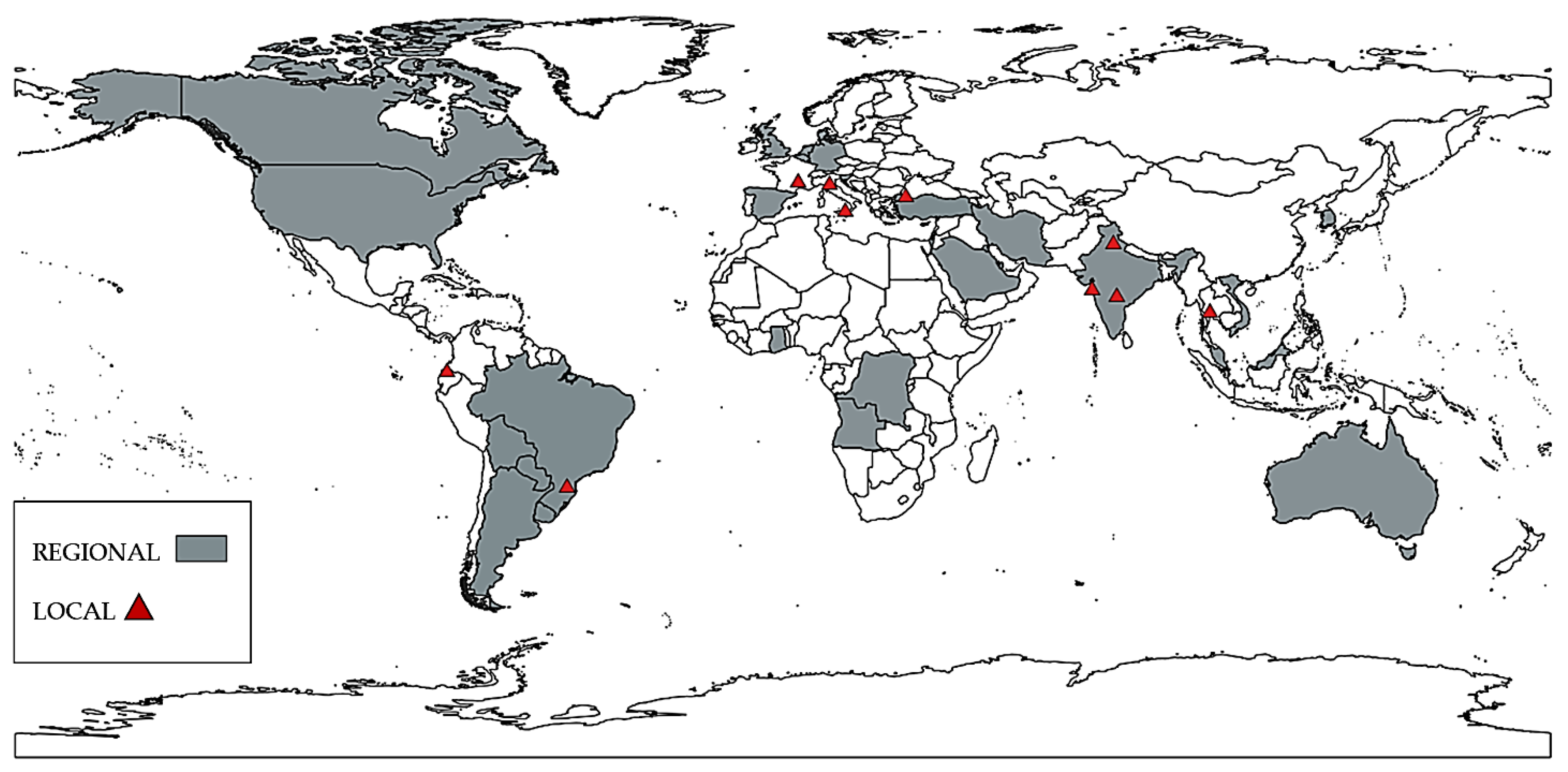
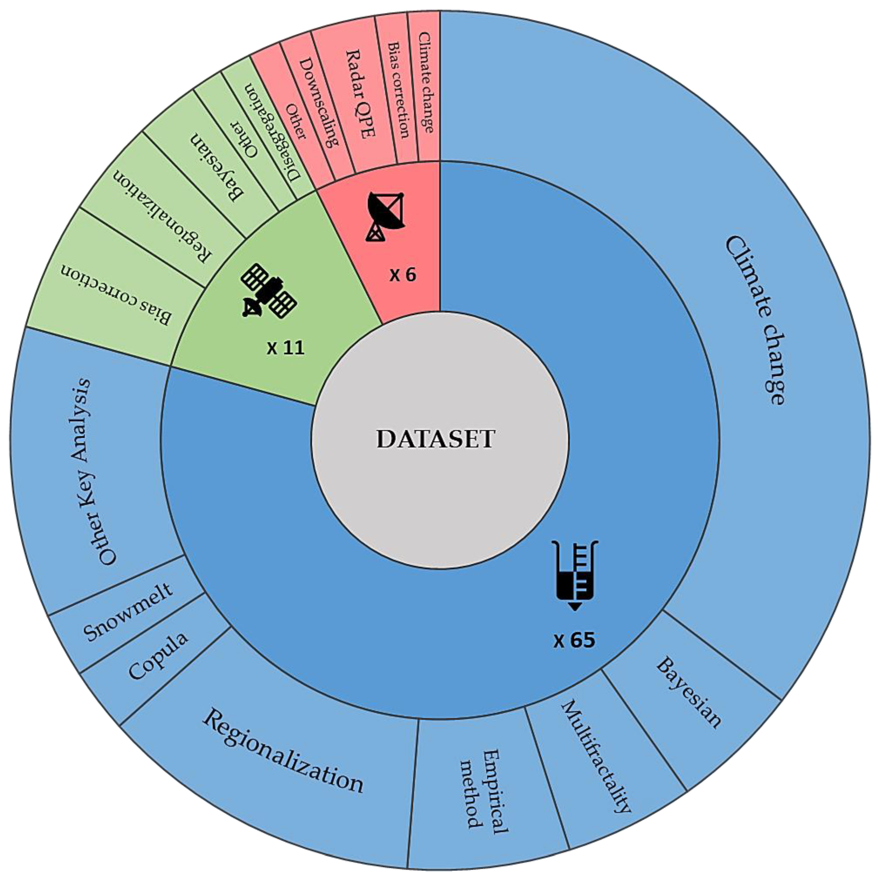
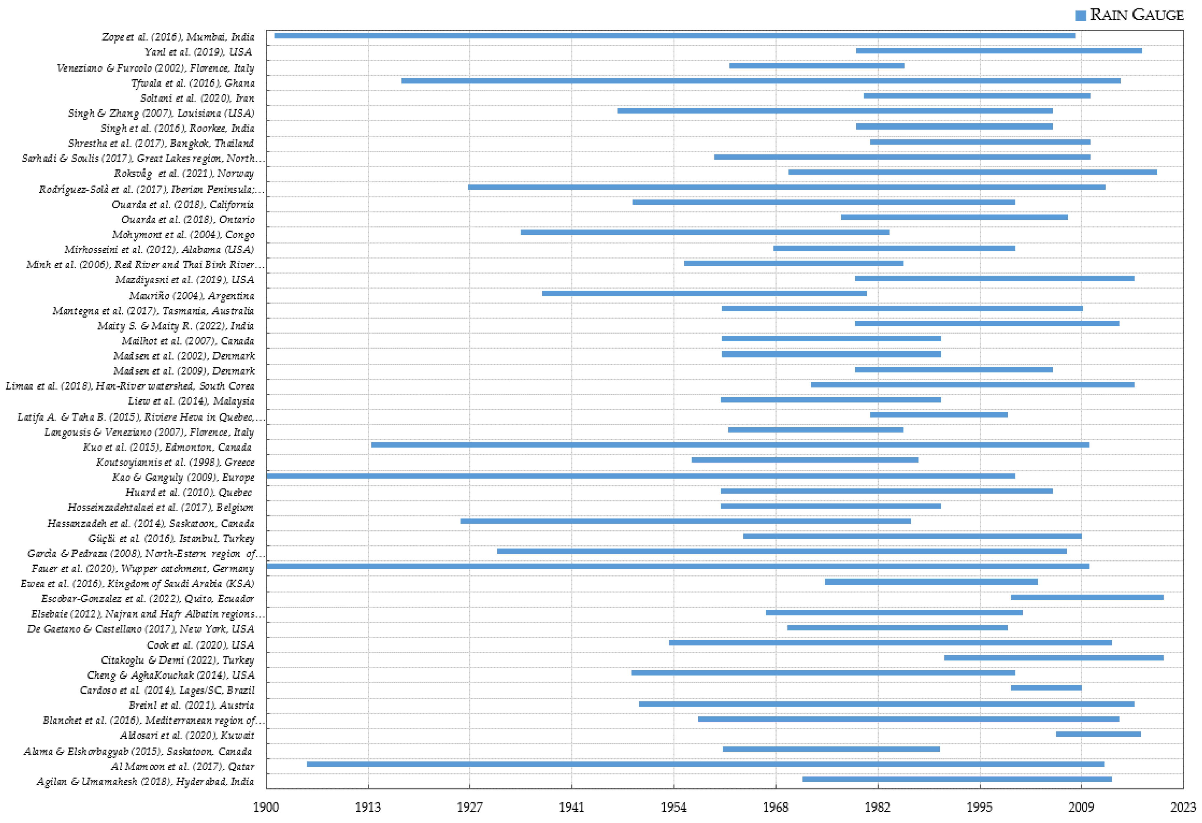
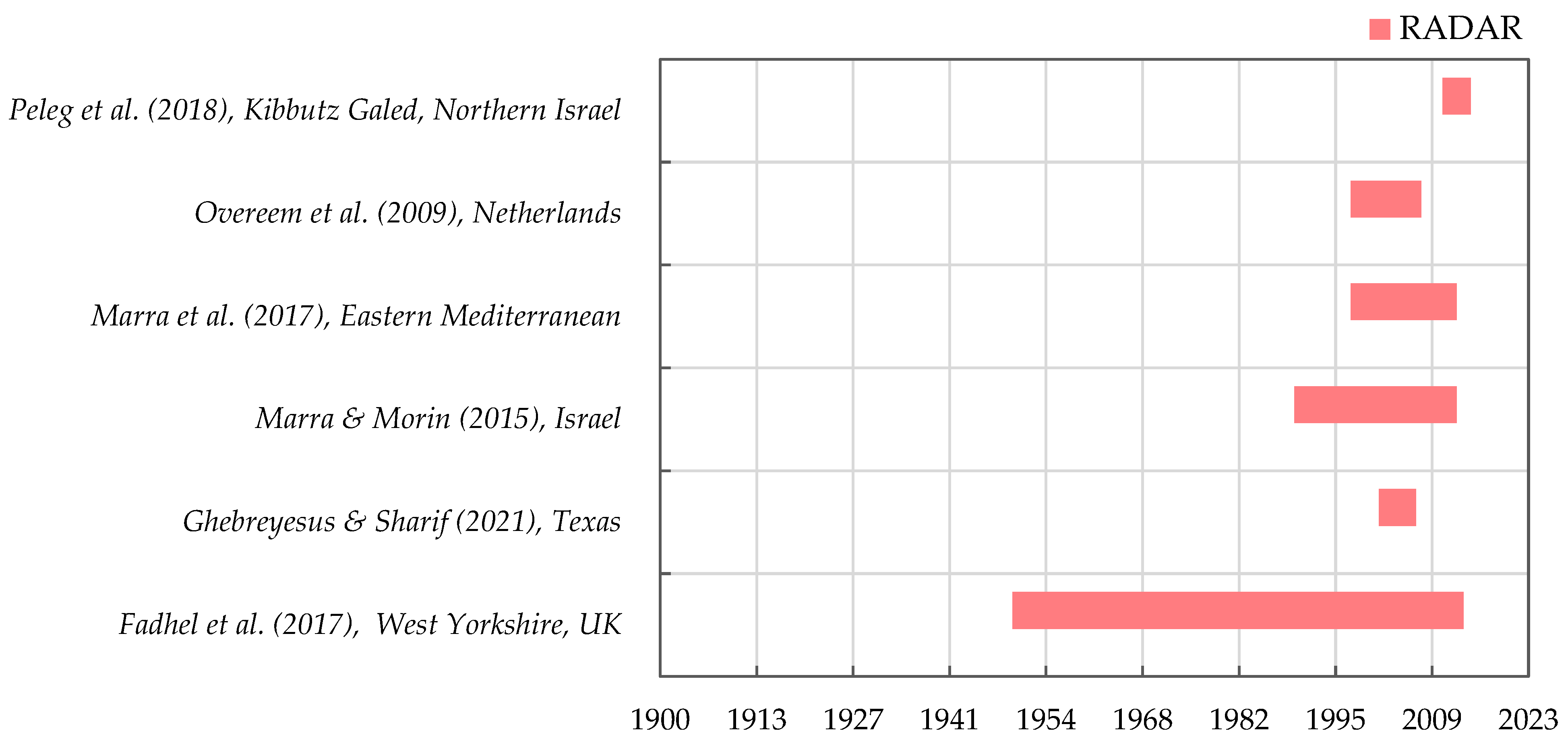
Table 1.
Search procedure used to identify relevant articles.
| Database | Category | Search Keywords | |
|---|---|---|---|
| Google Scholar | Dataset | Spatial scale | “Intensity–duration–frequency curves” & “radar” & “Continent” OR “Country” OR “Basin”; |
| “Intensity–duration–frequency curves” & “satellite” & “Continent” OR “Country” OR “Basin”; | |||
| “Intensity–duration–frequency curves” & “rain gauge” & “Continent” OR “Country” OR “Basin” | |||
| Climate Change | “Intensity–duration–frequency curves” & “radar” & “climate change”; | ||
| “Intensity–duration–frequency curves” & “satellite” & “climate change”; | |||
| “Intensity–duration–frequency curves” & “rain gauge” & “climate change” | |||
Table 2.
Papers developing IDFs using a rain-gauge dataset.
| Reference | Target | Key Analysis | Years (Observations) | Uncertainty | Location | Spatial Scale |
|---|---|---|---|---|---|---|
| Agilan & Umamahesh (2017) | Develop non-stationary IDFs using five physical processes, including urbanization and climate change, as covariates | Covariates | 1972–2013 | - | Hyderabad (India) | Local |
| Al Mamoon et al. (2017) | Assessing the influence of climate change on the IDF relationship for Qatar | Climate Change | 1962–2012 | - | Qatar | Regional |
| Aldosari et al. (2020) | Reconstruct the IDF curves for the urban area of the State of Kuwait using historical rainfall intensity data | Periodogram technique | 2006–2017 | - | Kuwait | Regional |
| Aron et al. (1987) | Define the IDF curves for each homogeneous rainfall region of the Pennsylvania territory to evaluate the design storms | Regionalization | - | - | Pennsylvania (USA) | Regional |
| Baghirathan & Shaw (1978) | Rainfall depth-duration-frequency studies for Sri Lanka with data of historic records of annual maximum rainfall depths | Regionalization | - | - | Sri Lanka | Local |
| Bell (1969) | Show that DDF curves have surprisingly consistent values in such diverse places as Alaska, Hawaii, Puerto Rica, South Africa, Australia and contiguous United States | Empirical method | - | - | Alaska, South Africa, Australia, USA | Regional |
| Bezak et al. (2017) | Combines empirical rainfall thresholds and IDF curves to develop early warning systems (EWS) in hazardous area of debris flows or landslides | Copula function | - | - | Slovenia | Regional |
| Blanchet et al. (2016) | Propose an integrated derivation of IDF relationships in the context of distributed GEV maxima, validated at regional scale | Regionalization | 1958–2014 | - | Cévennes (France) | Regional |
| Breinl et al. (2021) | Compare intensity-duration-frequency statistics of maximum annual precipitation with those of maximum annual streamflow | Quantiles from IDF models | 1950–2016 | - | Austria | Regional |
| Citakoglu & Demi (2022) | Carry out regional IDF equality using IDF relationship obtained from point frequency analysis | Optimization and Multi-Genetic-Programming methods | 1991–2020 | - | Turkey | Regional |
| Cardoso et al. (2014) | Analyze the frequency distribution and intensity temporal variability of intense rainfall for Lages/SC | Empirical method | 2000–2009 | - | Lages/SC (Brazil) | Local |
| Cheng & AghaKouchak (2014) | Use Bayesian-structured inference to develop the nonstationary IDF curves and assess their uncertainty | Bayesian inference | 1949–2000 | Yes | USA | Regional |
| Cook et al. (2020) | Analyze the effect of the spatial resolution of the regional climate model and the spatial adjustment technique on the updated IDF curves for climate change | Climate Change | 1954–2013 | - | USA | Regional |
| De Gaetano & Castellano (2017) | Develop a series of future extreme precipitation probabilities by downscaling and climate model projections | Downscaling (Climate Change) | 1970–1999 | - | New York | Local |
| Elsebaie (2012) | Derive IDF relationship of rainfall at Najran and Hafr Albatin regions in the kingdom of Saudi Arabia (KSA) | Regionalization | 1967–2001 | - | KSA (South Arabia) | Regional |
| Escobar-Gonzalez et al. (2022) | Develop an approach to build IDFs in the urban area of high-altitude Andean cities | 3-parameter mnp methodology for extreme events correction | 2000–2020 | - | Quito (Ecuador) | Local |
| Ewea et al. (2016) | Development of regional IDF formulas and curves for 13 administrative regions for the Kingdom of Saudi Arabia (KSA) and a global IDF curve for the entire country | Regionalization | 1975–2003 | - | KSA (South Arabia) | Regional |
| Fauer et al. (2020) | Look for new parametric forms of IDF curves that are applicable to a large range of durations | Empirical method | 1893–2010 | Yes | Germany | Regional |
| Ganguli & Coulibaly (2017) | Analyze the non-stationarity and trends of short-duration precipitation extremes in urbanized locations and evaluate the potential of non-stationary IDF curves | Climate Change | - | Yes | South Ontario | Regional |
| Garcìa & Pedraza (2008) | Analyze the temporal variation in the total number of days a year with rainfall above the 100 mm threshold at the rain gauging stations in NEA | Singular spectral analysis | 1931–2007 | - | North-Estern region (NEA) of Argentina | Regional |
| Güçlü et al. (2016) | Deriving IDF curves according to climate change scenarios at the Florya rainfall station in Istanbul, Turkey | Climate Change | 1964–2009 | - | Istanbul | Local |
| Hassanzadeh et al. (2014) | Use of the quantile-based downscaling technique to derive future IDF curves under climate change scenarios | Climate Change | 1926–1986 | Yes | Saskatoon | Local |
| Hosseinzadehtalaei et al. (2017) | Analyze the uncertainty of future IDFs using a variance decomposition technique and study the influence of the spatial resolution of RCMs | Downscaling (Climate Change) | 1961–1990 | - | Belgium | Regional |
| Huard et al. (2010) | Analysis and estimation of uncertainties of IDF curves using a Bayesian inference analysis | Bayesian inference | 1961–2005 | Yes | Québec | Regional |
| Kao & Ganguly (2011) | Characterize the non-stationary behavior of precipitation extremes under climate change scenarios | Climate Change | 1900–2000 | Yes | Europe | Regional |
| Kourtis & Tsihrintzis (2022) | Review the studies performed on updating IDF curves in the presence of climate change | Climate Change | - | Yes | - | - |
| Koutsoyiannis et al. (1998) | Propose a general formula for IDFs consistent with the probabilistic theoretical basis of rainfall maxima analysis | Regionalization/account for non-recording station | 1957–1987 | - | Greece | Regional |
| Kuo et al. (2015) | Derive IDF curves over the observation period and simulate future IDFs by estimating future slopes of air temperature and rainfall trends | Climate Change | 1914–2010 | Yes | Edmonton | Local |
| Langousis & Veneziano (2007) | Develop methods to estimate the IDF curves for three rainfall models with local multifractal behavior and varying complexity | Multifractality | 1962–1985 | - | Florence | Local |
| Latifa & Taha (2015) | Propose a methodology for developing IDFs using the covariates of climate indices | Climate Change | 1981–1999 | - | Rivière–Héva | Local |
| Liew et al. (2014) | Derive IDF curves by interpolating data from regions of climatologically similar characteristics for the ungauged site of Peninsular Malaysia | Climate Change | 1961–1990 | - | Malaysia | Regional |
| Limaa et al. (2018) | Estimate the parameters of a generalized distribution of extreme values on a sub-daily scale to derive current and future regional IDFs | Climate Change | 1973–2016 | Yes | South Corea | Regional |
| Madsen et al. (2002) | Regional estimation of IDF curves using the generalized least-squares regression method of short duration statistics | Regionalization | 1961–1990 | - | Denmark | Regional |
| Madsen et al. (2009) | Updating the IDF curves from the previous work in order to analyze any changes or trends in extreme precipitation | Regionalization | 1979–2005 | Yes | Denmark | Regional |
| Mailhot et al. (2007) | Analyze Canadian Regional Climate Model simulations and derive regional IDF curves at grid box and rainfall station scales | Climate Change | 1961–1990 | - | Canada | Regional |
| Maity S. & Maity R. (2022) | Investigate spatiotemporal changes in IDF relationship | Climate Change | 1979–2014 | Yes | India | Regional |
| Mantegna et al. (2017) | Examine the ability of the Conformal Cubic Atmospheric Model (CCAM) to reproduce sub-daily IFD curves | Climate Change | 1961–2009 | - | Tasmania | Regional |
| Martel et al. (2021) | Review the state of the art and guidelines for the adaptation of IDF curves to climate change | Climate Change | - | Yes | - | - |
| Mauriño (2004) | Compare the generalized rainfall intensity-duration-frequency relationships proposed by Bell (1969) with IDFs | Empirical method | 1937–1980 | - | Argentina | Regional |
| Mazdiyasni et al. (2019) | Propose a multivariate approach to construct heat wave intensity, duration, frequency (HiDf) curves | Multivariate Copula functions | 1979–2016 | - | USA | Regional |
| Minh et al. (2006) | Propose a generalized IDF formula using base rainfall depth and base return period for the monsoon region of Vietnam | Regionalization | 1956–1985 | - | Vietnam | Regional |
| Mirhosseini et al. (2013) | Develop future IDFs under climate change scenarios by applying the technique of dynamic downscaling of GCMs by RCMs | Climate Change | 1968–2000 | Yes | Alabama (USA) | Regional |
| Mohymont et al. (2004) | Produce IDF-curves for three different climatological stations in Congo in Central Africa | Empirical method | 1934–1983 | - | Congo | Regional |
| Neelin et al. (2022) | Examining precipitation extremes and water vapor relations in the current climate and implications for climate change | Climate Change | - | - | - | - |
| Ouarda et al. (2018) | Define non-stationarity IDFs integrating information concerning teleconnections and climate change | Climate Change | 1977–2007 | - | Ontario | Regional |
| Ouarda et al. (2018) | Climate Change | 1949–2000 | - | California | Regional | |
| Ragno et al. (2018) | Estimate climate change impacts on extreme rainfall magnitude and frequency using bias corrected historical and multi-model projected precipitation extremes | Bayesian inference | - | Yes | USA | Regional |
| Rodríguez-Solà et al. (2016) | Analyze of the structure of rainfall in the Mediterranean area, taking into account geographical and climate characteristics also | Multifractality | 1927 –2012 | - | Iberian Peninsula, Balearic Islands | Regional |
| Roksvåg et al. (2021) | Develop accurate and consistent IDFs by post-processing of Bayesian-estimated IDF curves and by a non-parametric and consistent IDF relationship | Bayesian inference | 1970–2019 | - | Norway | Regional |
| Sandink et al. (2016) | Analyze stakeholder engagement to support the development of a computerized tool that develops future IDFs under climate change | Climate Change | - | Yes | Canada | Regional |
| Sarhadi & Soulis (2017) | Incorporate the impact of several complex non-stationary conditions on the occurrence of extreme precipitation in the Great Lakes area | Downscaling (Climate Change) | 1960–2010 | - | Great Lakes region (North America) | Regional |
| Shahabul Alam & Elshorbagy (2015) | Develop future IDFs under climate change scenarios based on continuous rainfall records | Climate Change | 1961–1990 | Yes | Saskatoon | Local |
| Shehu et al. (2022) | Investigate the use of different data types and methods for estimating reliable DDF curves covering whole Germany | Regionalization | - | - | Germany | Regional |
| Shrestha et al. (2017) | Develop future IDFs using a stochastic weather generator and a rainfall disaggregation tool, for Bangkok area in Thailand | Downscaling (Climate Change) | 1981–2010 | Yes | Bangkok | Local |
| Simonovic et al. (2016) | Standardize the IDF update process by a web-based tool for the development of Intensity Duration Frequency curves under changing climate | Climate Change | - | Yes | Canada | Regional |
| Simonovic et al. (2016) | Develop a web-based tool to update IDF curves according to climate change | Climate Change | - | Yes | Canada | Regional |
| Singh et al. (2016) | Update IDF curves for a typical Indian town using an ensemble of five General Circulation Models | Climate Change | 1979–2005 | - | Roorkee (India) | Local |
| Singh & Zhang (2007) | Derive IDF curves from bivariate rainfall frequency analysis using the Frank Archimedean Copula method | Multifractality | 1947–2005 | - | Louisiana | Regional |
| Sivapalan & Bloeschl (1999) | Present an alternative methodology based on the spatial correlation structure of rainfall for IDFs | Transform point rainfall in areal rainfall | - | - | Austria | Regional |
| Soltani et al. (2020) | Introduce a new method for projecting short-time rainfall IDF through a regional scale to estimate short-term rainfall at ungagged basins | Climate change | 1981–2010 | Yes | Iran | Regional |
| Tfwala et al. (2016) | Deriving IDFs from a nearly 100-year-long rainfall data set in the Ghaap Plateau, Northern Cape Province, South Africa | IDF uncertainties estimation | 1918–2014 | Yes | Ghana | Regional |
| Veneziano & Furcolo (2002) | Derivation of scaling properties of IDF curves considering precipitation as a stationary multifractal process | Multifractality | 1962–1985 | - | Florence | Local |
| Yanl et al. (2018) | Propose next-generation IDF curves that consider the actual water reaching the land surface, including snow melt | Include snowmelt contribution | - | - | USA | Regional |
| Yanl et al. (2019) | Compare peak design flood values computed by traditional method and new generation IDFs in the western United States | Include snowmelt contribution | 1979–2017 | USA | Regional | |
| Zope et al. (2016) | Develop IDF rainfall curves for the Mumbai city using longer length of observed rainfall data | New IDF relationship for Mumbai | 1901–2008 | - | Mumbai | Local |
Table 3.
Papers developing IDFs using a radar dataset.
| Reference | Target | Key Analysis | Years (Observations) | Uncertainty | Location | Spatial Scale |
|---|---|---|---|---|---|---|
| Fadhel et al. (2017) | Derivation of IDF curves under climate change scenarios, by daily precipitation data simulated with 1-km regional climate model | Statistical bias correction method; Disaggregation model | 1950–2014 | Yes | West Yorkshire (UK) | Regional |
| Ghebreyesus & Sharif (2021) | Use the high-resolution US NationalWeather Service (NWS) Next Generation Weather Radar (NEXRAD) Stage-IV precipitation data to develop IDFs with a high spatial resolution in Texas | Exceedance probability for radar pixels | 2002–2020 | - | Texas (USA) | Regional |
| Marra & Morin (2015) | Use of radar quantitative precipitation estimation (QPE) for the identification of IDF curves over a region with steep climatic transitions | Radar QPE | 1990–2013 | Yes | Israel | Regional |
| Marra et al. (2017) | Quantify subpixel variability of extreme rainfall by using a novel space–time rainfall generator that downscales in space the rainfall within a given radar pixel | Non-dimensional normalized metrics | 1998–2013 | Yes | Eastern Mediterranean | Regional |
| Overeem et al. (2009) | Derivation of depth-duration-frequency (DDF) curves from radar data for The Netherlands | Radar QPE | 1998–2008 | - | Netherlands | Regional |
| Peleg et al. (2018) | Building Radar-IDF curves and IDF curves based on point representing the radar subpixel extreme rainfall variability | Downscaling | 2011–2015 | - | Gal’ed (Northern Israel) | Regional |
Table 4.
Papers developing IDFs using a satellite dataset.
| Reference | Target | Key Analysis | Years (Observations) | Uncertainty | Location | Spatial Scale |
|---|---|---|---|---|---|---|
| AghaKouchak et al. (2011) | Analysis of satellite data to assess the best performing in capturing precipitation extremes | Monthly Quantile Bias (MQB) | 2005–2008 | - | USA | Regional |
| Ayman et al. (2011) | Development of IDF curves by mixing ground rainfall stations data and satellite data for a region with limited rainfall records | Regionalization | 1998–2008 | - | North-West of Angola | Local |
| Bertini et al. (2020) | Calculate intensity–duration–area–frequency (IDAF) curves and estimate the design peak discharge for a dam watershed whose spillway design lenght length is to be determined | Regionalization | 2002–2017 | Yes | Catania | Local |
| Courty et al. (2019) | Study global-scale IDF relationships using a gridded, multitemporal resolution precipitation dataset to estimate rainfall intensity for a continuous range of durations | Scaling of distribution parameters | 1979–2018 | - | United Kingdom | Regional |
| Endreny & Imbeah (2009) | Evaluating the predictive value of freely available short duration satellite records combined with limited ground-based measured data in a frequency analysis method designed for robust estimation of rainfall IDF | Global and Regional frequency method | 1998–2006 | - | Ghana | Regional |
| Hosseinzadehtalaei et al. (2020) | Update of IDF curves based on the impact of climate change on extreme short-duration precipitation in Europe | Bayesian approach | 1971–2000 | Yes | Europe | Regional |
| Islam et al. (2022) | Provide a viable alternative to estimate unbiased IFD curves at the sub-hourly timescale by a novel framework, SIFD (Satellite-derived IFD curves) to combine long-term daily gauge data and sub-hourly SPP | Bayesian Generalised Least Squares Regression; Regionalization | 2001–2019 | - | Australia | Regional |
| Marra et al. (2017) | Quantify subpixel variability of extreme rainfall by using a novel space–time rainfall generator that downscales in space the rainfall within a given radar pixel | Non-dimensional normalized metrics | 1998–2013 | Yes | Eastern Mediterranean | Regional |
| Noor et al. (2021) | To generate reliable IDFs by analyzing the performance of four remote sensing-based gridded rainfall data processing algorithms | Bias correction | 2000–2018 | - | Malaysia | Regional |
| Ombadi et al. (2018) | Development of basin-scale IDFs on the contiguous United States (CONUS) by the transformation of precipitation from areal to point | Bias correction | 1983–2018 | Yes | USA | Regional |
| Sun et al. (2019) | Development of more reliable IDF curves from satellite data by the disaggregation of daily in situ rainfall for Singapore city | Disaggregation hourly rainfall | 1998–2010 | Yes | Singapore | Local |
Publisher’s Note: MDPI stays neutral with regard to jurisdictional claims in published maps and institutional affiliations. |
© 2022 by the authors. Licensee MDPI, Basel, Switzerland. This article is an open access article distributed under the terms and conditions of the Creative Commons Attribution (CC BY) license (https://creativecommons.org/licenses/by/4.0/).
Share and Cite
MDPI and ACS Style
Lanciotti, S.; Ridolfi, E.; Russo, F.; Napolitano, F. Intensity–Duration–Frequency Curves in a Data-Rich Era: A Review. Water 2022, 14, 3705. https://doi.org/10.3390/w14223705
AMA Style
Lanciotti S, Ridolfi E, Russo F, Napolitano F. Intensity–Duration–Frequency Curves in a Data-Rich Era: A Review. Water. 2022; 14(22):3705. https://doi.org/10.3390/w14223705
Chicago/Turabian StyleLanciotti, Sabrina, Elena Ridolfi, Fabio Russo, and Francesco Napolitano. 2022. "Intensity–Duration–Frequency Curves in a Data-Rich Era: A Review" Water 14, no. 22: 3705. https://doi.org/10.3390/w14223705
Note that from the first issue of 2016, this journal uses article numbers instead of page numbers. See further details here.