Seasonal Variation of Intra-Seasonal Eddy Kinetic Energy along the East Australian Current

Abstract

By using satellite altimeter observations and the eddy-permitting Estimating the Circulation and Climate of the Ocean, Phase II (ECCO2), the seasonal variation of eddy kinetic energy (EKE) along the East Australian Current (EAC) is investigated. Both observations and ECCO2 outputs indicate active intra-seasonal EKE along the EAC path. The ECCO2 result reveals that the intra-seasonal EKE is mainly concentrated in the upper 500 m layer, and shows a prominent seasonal cycle, strong in austral summer and weak in austral winter. Eddy energy budget diagnosis reveals that the evolution of EKE is controlled by barotropic instability of the mean EAC. The seasonal variation of baroclinic instability is opposite to the barotropic instability variation, but of a much smaller magnitude. Further analysis indicates that the seasonal cycle of mesoscale signals in this region is related to the transport variability of the EAC.

1. Introduction

The East Australian Current (EAC) is one of the most important current systems in the South Pacific Ocean. It carries huge amount of warm water from low latitudes to high latitudes, significantly affecting the local climate (Bowen et al., 2006 [1]; Speich et al., 2002 [2]). Besides, located at a crossroad between the Pacific and the Indian Oceans, the EAC also affects the material transport across the basins (Ridgway and Godfrey, 1997 [3]). Therefore, it is of great importance to study the dynamic processes of the multi-scale circulation variability in the EAC region. Compared to the other western boundary currents, the EAC is less explored, especially in terms of its eddy–mean flow interaction (Imawaki et al., 2013 [4]).

The EAC occupies a region of complex ocean dynamics characterized by current bifurcations and eddy shedding (Figure 1). The EAC is formed at 10–15° S, and it gradually intensifies poleward (Ridgway and Dunn, 2003 [5]). At about 32° S, the EAC separates into two branches: one, referred to as the southward EAC extension, and the other, the eastward Tasman Front, due to a combined effect of nonlinear flow instabilities and upper-ocean-topographic coupling (Tilburg et al., 2001 [6]). Based on historical hydrographic observations and expendable bathythermograph data, Ridgway and Godfrey (1997 [3]) firstly showed the seasonal variation in the EAC, with an amplitude of 6 Sv, weaker in austral winter and stronger in austral summer. Subsequent studies also revealed significant seasonal variations of the EAC’s southward transport (Cetina-Heredia et al., 2014 [7]) and its cross-shelf transport (Schaeffer et al., 2014 [8]) by using in situ and satellite data, as well as model outputs. The stronger EAC in austral summer is associated with higher eddy kinetic energy (EKE) in this region (Qiu and Chen, 2004 [9]) and a southward shift of the EAC separation latitude (Ypma et al., 2016 [10]). Nevertheless, by using Argo data and satellite altimeter observations, Zilberman et al. (2018) [11] suggested that the EAC transport reaches its peak in March (21.6 ± 1.4 Sv), much earlier than previous studies. All these studies reveal the complex ocean dynamics of the seasonal variability in the EAC.

Although the EAC is recognized to be the weakest western boundary current in the ocean, its regional mesoscale eddy activities are comparable with those in the Gulf Stream and the Kuroshio, and play a vital role in the EAC system (Mata et al., 2006 [12]). By using satellite altimeter observations, previous studies have found significant oscillations in the EAC transport with periods between 90 and 180 days, and suggested that it is associated with eddy activities in this region (Bowen et al., 2005 [13]; Mata et al., 2006 [12]; Wilkin and Zhang, 2007 [14]). Based on observations and model outputs, eddy shedding activities in the EAC separation latitude have been explored (Everett et al., 2012 [15]), and the result reveals that these eddies have a major impact on the entrainment and connectivity of plankton and fish populations. Besides, van Sebille et al. (2012) [16] found that the detached eddies could move southward and eventually enter the Indian Ocean, affecting the heat and mass transport between the ocean basins. In addition to these shedding eddies, previous studies also found significant eddy activities in the southwest Pacific (Bowen et al., 2006 [1]), which are related to the baroclinic instability along the South Pacific Subtropical Countercurrent (Qiu and Chen, 2004; Travis and Qiu, 2017 [17]).

Previous research has focused on the seasonal variability in the EAC, especially the southward EAC transport, but less attention has been paid to how these seasonal variations of circulation impact on the mesoscale eddy activities along the EAC path. As the EAC varies with season, its horizontal velocity shear and its separation latitude all fluctuate. All these changes could modify the stability of the EAC system, affecting potentially the mesoscale eddy-shedding activities. To explore this modification, both satellite altimeter observations and outputs from a global eddy-permitting ECCO2 state estimate are used in this study. The goal is to detect the intra-seasonal eddy modulations along the EAC path and to quantify the related dynamical processes on the seasonal time scale.

2. Data and Methods

2.1. Observation Data

Gridded AVISO (Archiving Validation and Interpretation of Satellite Data in Oceanography) absolute dynamic topography (ADT) data and absolute geostrophic velocities are used in this study, which are distributed by the European Copernicus Marine Environment Monitoring Service (http://marine.copernicus.eu/) (accessed on 1 October 2022). The data combines a number of altimeter measurements such as Jason-1, Jason-2, Jason-3, ERS-1/2, HY-2A and others. The horizontal resolution is 0.25° × 0.25° and the temporal resolution is one day. To verify the ECCO2 outputs, both ADT and absolute geostrophic velocities from January 1993 to October 2019 are utilized in this study.

2.2. ECCO2 State Estimate

Outputs from an eddy-permitting model-Estimating the Circulation and Climate of the Ocean-Phase II (ECCO2) is used to explore the variation of EKE in the upper layer (http://apdrc.soest.hawaii.edu/datadoc/ecco2_cube92.php) (accessed on 10 November 2020), which is based on the Massachusetts Institute of Technology general circulation model (MITgcm). The eddy-permitting ocean state estimate is obtained by a least squares fit of the MITgcm outputs to satellite and in situ observations, which include sea level anomaly, sea surface temperature, temperature/salinity profiles, sea surface wind and precipitation data (Menemenlis et al., 2005 [18]).

In this study, ECCO2 sea level, temperature, salinity, and velocity data from 1992 to 2019 are utilized to explore the seasonal variation of EKE along the EAC. All data have a horizontal resolution of 0.25° × 0.25° and a temporal resolution of three days. As an important indicator for measuring mesoscale signals in the ocean, EKE can be calculated as follows:

$$EKE=\left(u^{\prime 2}+v^{\prime 2}\right)/2$$

(1)

where $u^{\prime }$ and $v^{\prime }$ denote zonal and meridional velocity anomalies, which are defined as the difference of current with the annual mean current.

3. Verification of ECCO2 Simulation

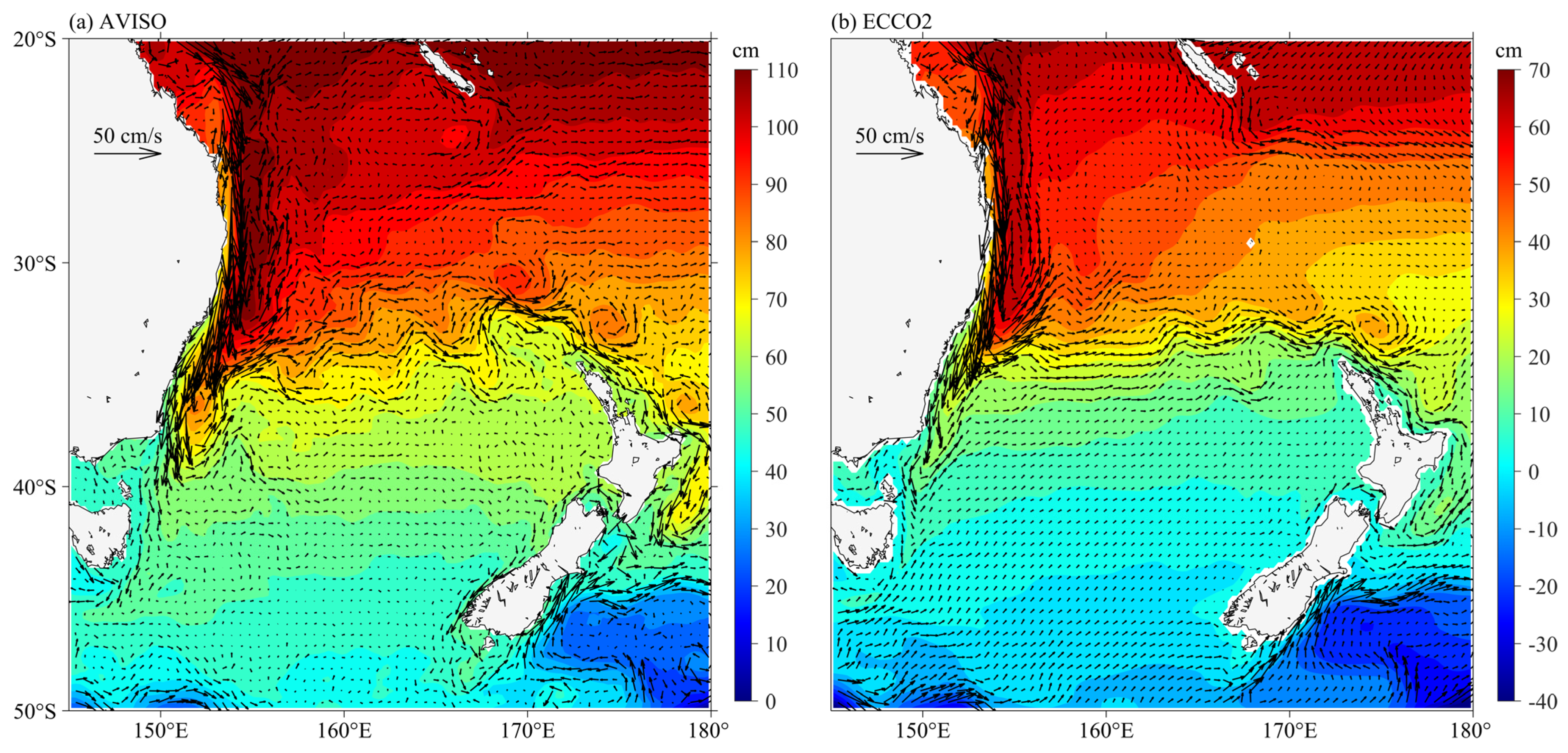
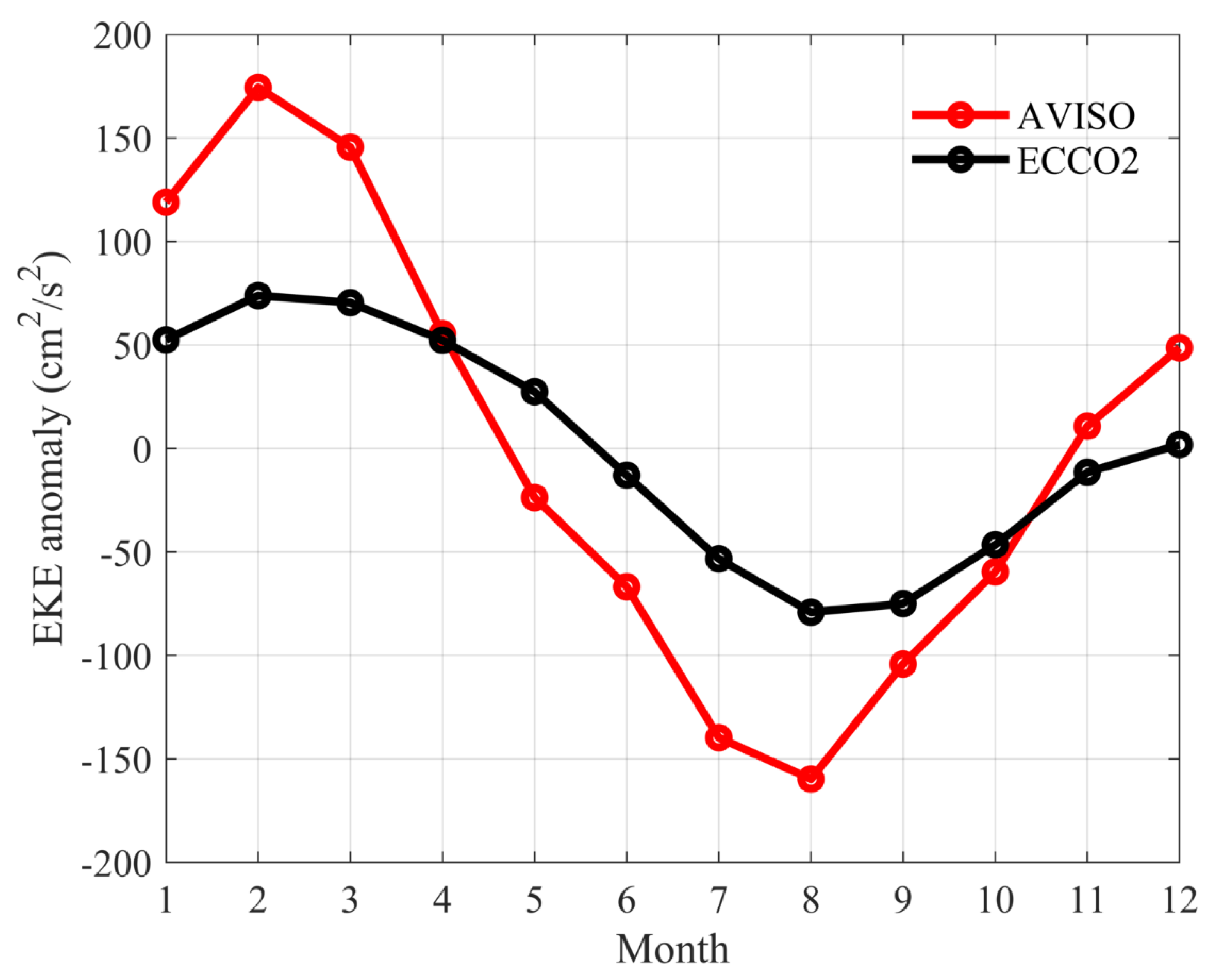
Before using the ECCO2 state estimate to study the dynamic processes governing the EKE signals in the EAC region, it is important to assess the accuracy of ECCO2 outputs against the satellite altimetry observations. As shown in Figure 1, both SSH fields and surface circulations of ECCO2 state estimate match well that of AVISO data, which shows strong current retroflections associated with the positive SSH anomalies at about 37° S, and the meandering Tasman Front associated with the distinct SSH gradients along 34° S. Such good agreement is partially due to the assimilation of AVISO data in ECCO2 state estimate. In addition, we compared the time-mean surface EKE distributions in the EAC region, which are calculated from both AVISO data and ECCO2 outputs (Figure 2). The result indicates that the ECCO2 state estimate can simulate EKE signals along the EAC. Both AVISO and ECCO2 results show high EKE in the 150–160° E, 25–38° S (red box in Figure 2), around the EAC separation latitude, although the EKE signals from the ECCO2 outputs are relatively weaker to the south of 35° S. We also compared the observed and simulated EKE time series averaged in the high EKE region (red box in Figure 2) as a function of calendar months (Figure 3). It can be seen that both time series show an annual cycle that is strong in austral summer and weak in austral winter. Given these agreements, we believe the ECCO2 state estimate is reliable enough to explore the seasonal variation of EKE along the EAC.

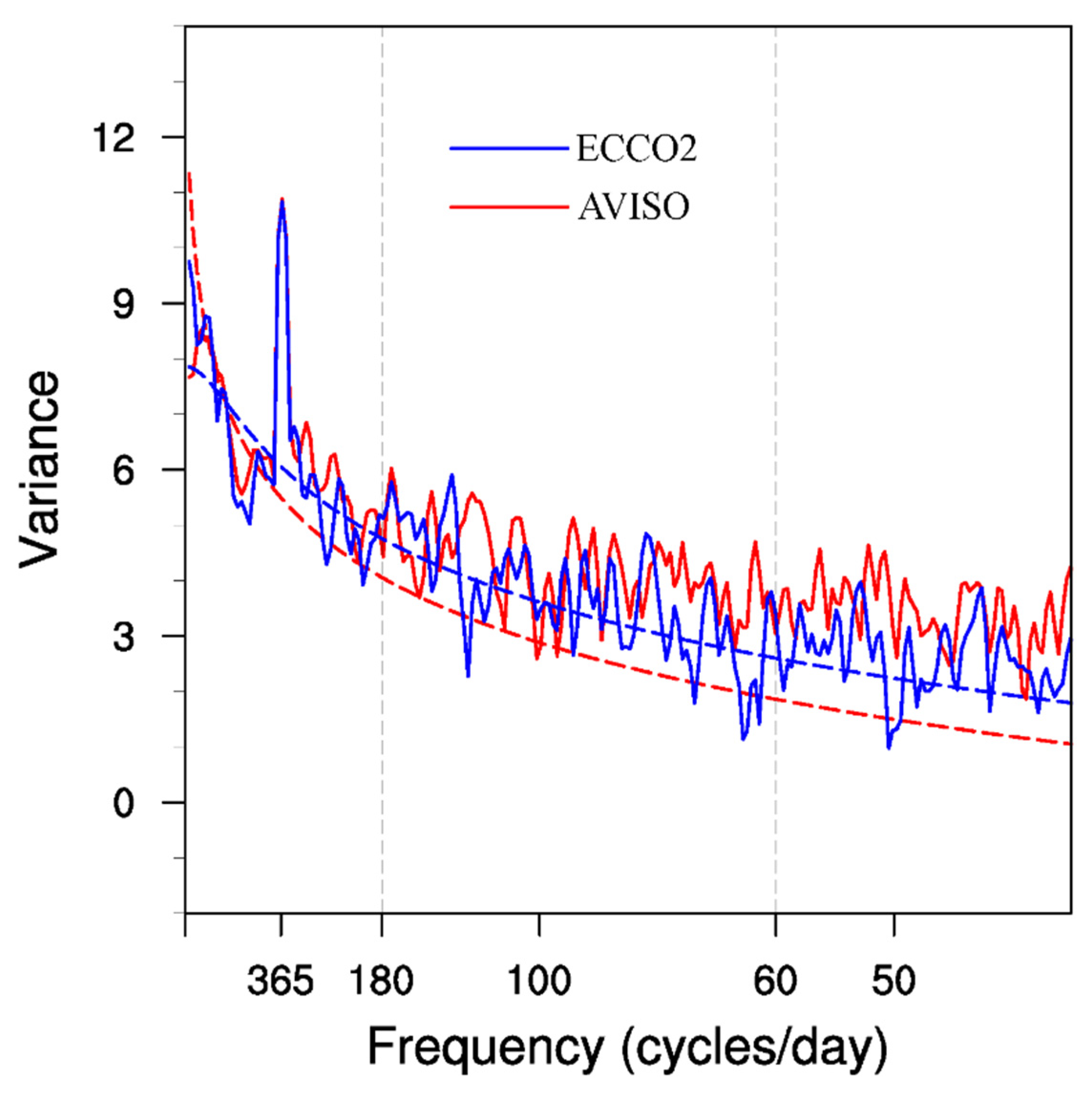
To better focus on the mesoscale signals, we calculated the variance-preserved power spectra of sea level anomalies along the EAC (red box in Figure 2) from the AVISO data and ECCO2 state estimate. As shown in Figure 4, in addition to the prominent annual period signals at 365 days, both observed and simulated results show significant intra-seasonal signals with periods at 60–180 days. To better focus on the intra-seasonal signals, we separate the velocity u into two parts, as follows:

$$u\left(x,y,t\right)=\tilde{u}\left(x,y,t\right)+u^{″}\left(x,y,t\right)$$

(2)

where, $\tilde{u}$ and $u^{″}$ denote the 180-day low-pass filtered velocity time series and 60–180-day bandpass filtered velocity time series, respectively. In this paper, a 4-order Butterworth filter is used to extract intra-seasonal signals.

4. Seasonal EKE Modulation along the EAC

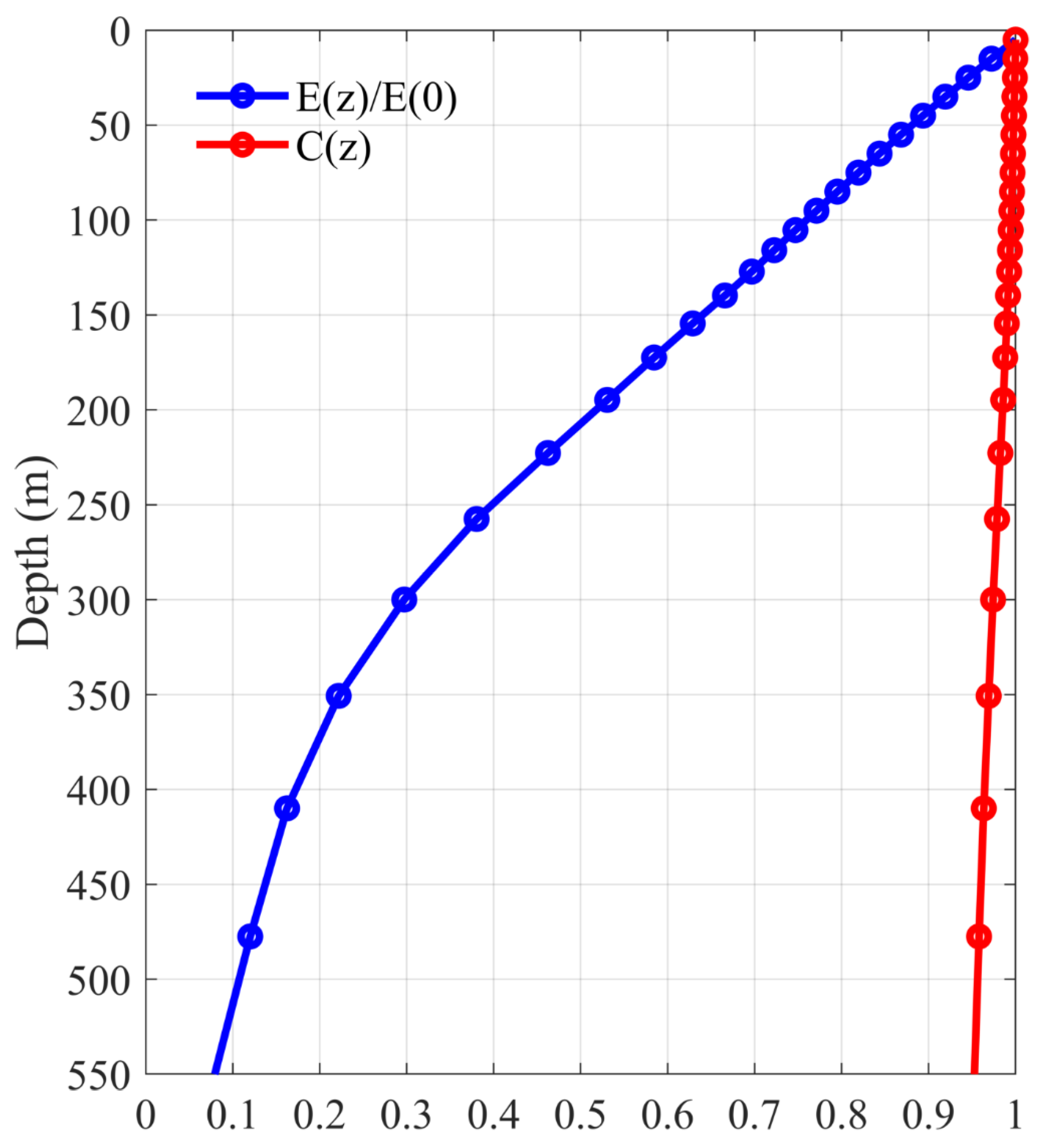
To explore the seasonal variation of EKE along the EAC, it is first necessary to determine the vertical structure of the EKE. To do so, we calculated the EKE time series at different depths from the ECCO2 outputs, referred to as E(t, z), which is spatial averaged in the chosen region (red box in Figure 2). As shown in Figure 5, the blue line represents the ratio of EKE at different depths to EKE at the surface: 〈E(t, z)〉/〈E(t, 0)〉, where 〈 〉 represent the time mean result. It can be seen that the EKE ratio decreases rapidly with depth. At about 500 m, the EKE value is only 10 percent the size of surface EKE. The red line represents the correlation coefficient between the EKE time series at different depths and the surface time series, which is calculated as follows:

$$\mathrm{C}\left(\mathrm{z}\right)\equiv 1-\frac{\langle {\left[E\left(t,z\right)-r\left(z\right)E\left(t,0\right)\right]}^2\rangle }{\langle E^2\left(t,z\right)\rangle }$$

(3)

where, $r\left(z\right)\equiv \langle E\left(t,z\right)E\left(t,0\right)/E^2\left(\mathrm{t},0\right)\rangle$ is the regression coefficients. Here, C(z) represents the correlation between EKE time series at different depth z and the surface EKE time series. It can be seen that C(z) is greater than 0.9 over the full upper 500 m layer. This indicates that the temporal variation of EKE at different depth is similar to that at the surface. Given the ratio and correlation between E(t, 0) and E(t, z) at different depth, we focus below on the EKE variations in the upper 500 m layer.

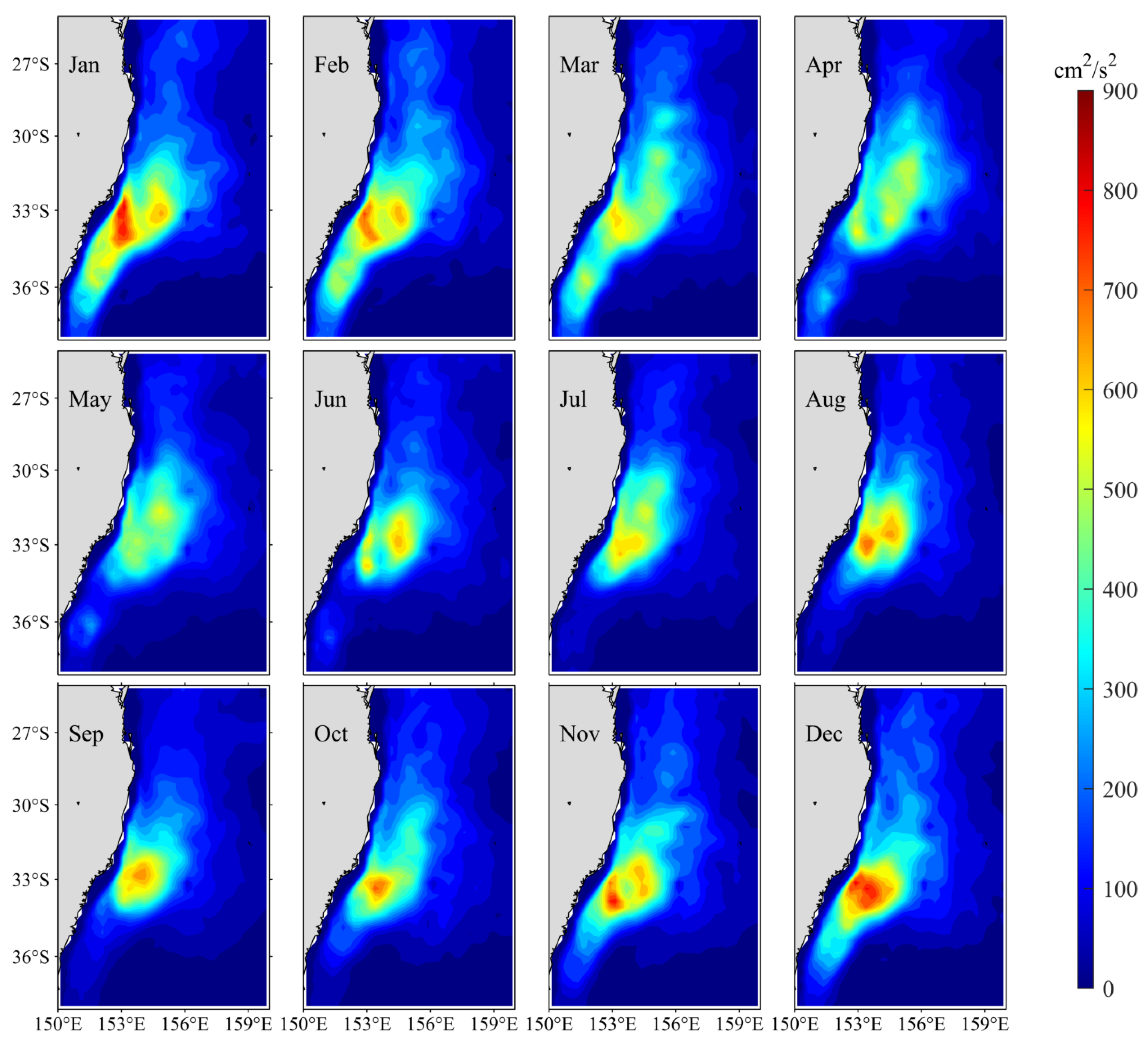
Figure 6 shows the monthly distribution of EKE along the EAC averaged in the upper 500 m, which is calculated by using 60–180-day bandpass filtered $u^{″}$ and $v^{″}$ based on Equation (1). The EKE is relatively larger around the EAC separation latitude, and shows a well-defined annual cycle. The EKE is largest in austral summer from December to February, with the maximum value area extends to south about 36° S. After February, the EKE decreases gradually and the maximum value area shrinks similarly. Both the EKE and the maximum value area reach their minima in June.

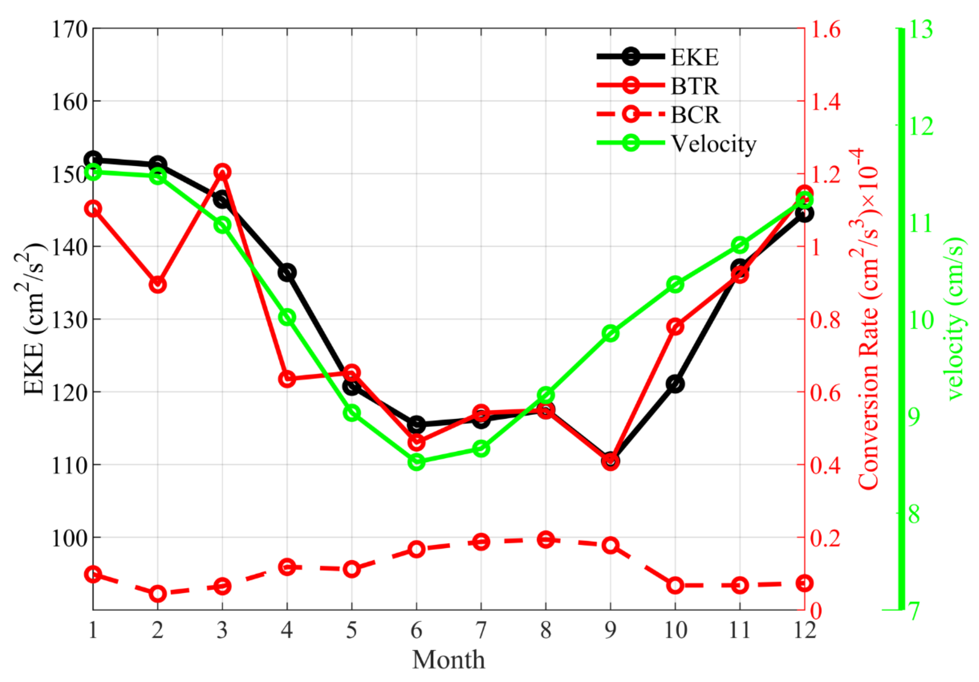
In Figure 9, we plot the mesoscale EKE time series (black line) in the 150–160° E, 25–38° S as a function of calendar months. With a maximum (152 cm²/s²) in January and a minimum (110 cm²/s²) in September, the seasonality of EKE along the EAC is clearly dominated by the local EKE signals around the EAC separation latitude.

5. Processes Governing the Seasonal EKE Variability

In order to elucidate the dynamic processes behind the seasonal variation of EKE, we calculated the barotropic and baroclinic eddy energy conversion rates, which are defined as follows (Chen et al., 2015 [19]; Yang et al., 2020 [20]):

$$\mathrm{barotropic}\mathrm{conversion}\mathrm{rate}=-\left(u^{″}{u}^{″}\frac{\partial \tilde{u}}{\partial x}+u^{″}{v}^{″}\left(\frac{\partial \tilde{v}}{\partial x}+\frac{\partial \tilde{u}}{\partial y}\right)+v^{″}{v}^{″}\frac{\partial \tilde{v}}{\partial y}\right)$$

(4)

$$\mathrm{baroclinic}\mathrm{conversion}\mathrm{rate}=-\left(\frac{g}{{\rho }_0}{\rho }^{″}{w}^{″}\right)$$

(5)

where, $u^{″}$ and $v^{″}$ are the 60–180-day bandpass filtered horizontal velocity anomalies, and $\tilde{u}$ and $\tilde{v}$ denote the background horizontal currents (including time–mean flows) with time scales longer than 180 days. Similarly, ${\rho }^{″}$ and $w^{″}$ are the 60–180-day bandpass filtered potential density and vertical velocity anomalies, g is the gravitational acceleration (g = 9.8 m/s²), ${\rho }_0$ is the background potential density (${\rho }_0$ = 1025 kg/m³). It should be noted that the barotropic conversion rate (BTR) represents the conversion process between EKE and mean kinetic energy (MKE). A positive BTR represents the conversion of energy from the MKE to the EKE, and reflects barotropic instability of the background mean flow. The baroclinic conversion rate (BCR) represents the transformation between eddy potential energy (EPE) and EKE. A positive baroclinic conversion rate represents the energy transformation from EPE to EKE as a result of baroclinic instability.

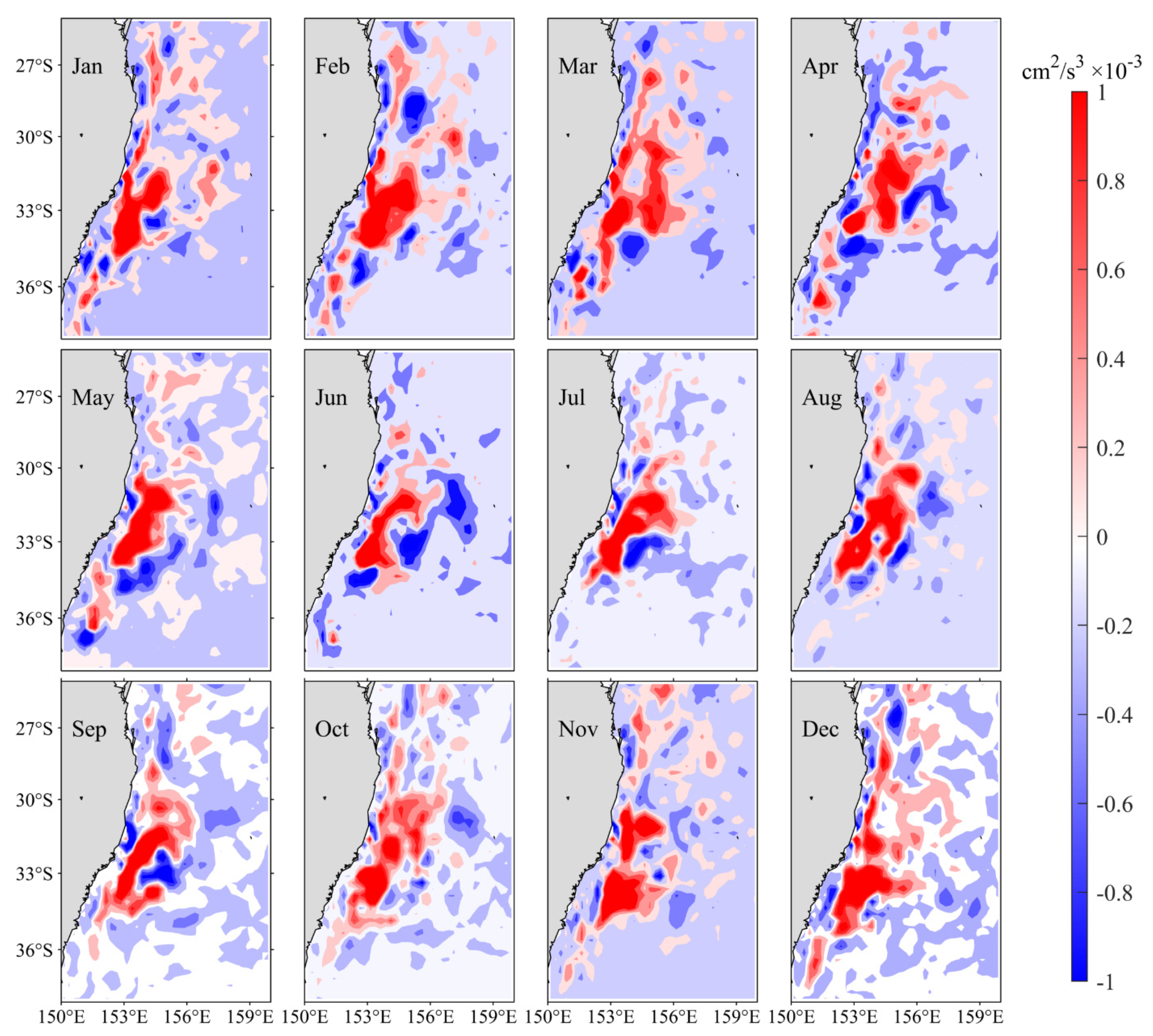
Figure 7 shows the monthly mean barotropic conversion rate (BTR) distributions averaged in the upper 500 m. the BTR is larger along the EAC path, especially around the EAC separation latitude. In addition, the BTR shows a clear seasonal variation. Starting from June, positive BTR signals increase in magnitude gradually until February and weaken steadily after March. Along with the seasonal evolution of the BTR, the maximum value area of positive BTR expands southward in austral winter and shrinks northward in austral summer. This seasonal variation of BTR matches favorably with the evolution in mesoscale EKE signals along the EAC (recall Figure 6).

Figure 9 plots the BTR time series (red solid line) as a function of calendar months, which are averaged within 150–160° E, 25–38° S region. The BTR is largest in March (1.2 × 10⁻⁴ cm²/s³) and smallest in September (0.4 × 10⁻⁴ cm²/s³). It can be seen that the seasonal variation of BTR is similar to the seasonal cycle of EKE, except for the drop-out value in February. Over all, this result reveals the high correlation between EKE and BTR.

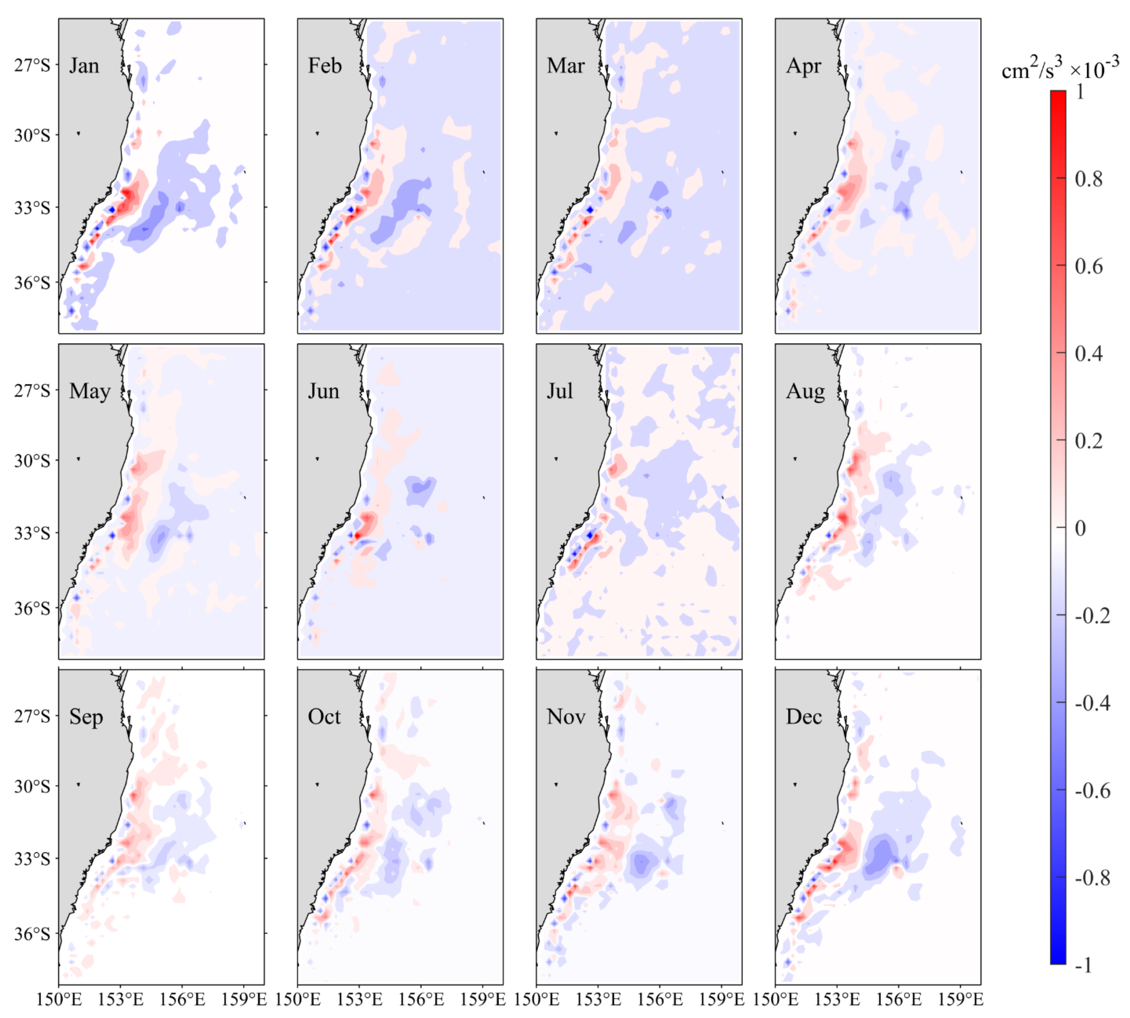
We also calculated the BCR variation in this study. Figure 8 shows the monthly distributions of the BCR averaged in the upper 500 m layer. Like BTR, the large BCR values are also concentrated in the EAC separation region. Moreover, BCRs are largely positive along the coast and negative in the offshore sea, forming a dipole structure. Overall, the BCR values are much smaller than BTR. The red dash line in Figure 9 shows the BCR time series in the 150–160° E, 25–38° S region as a function of calendar months. It is largest (0.19 × 10⁻⁴ cm²/s³) in August and smallest (0.04 × 10⁻⁴ cm²/s³) in February, which is opposite to the seasonal BTR variation. In general, the seasonal variation of BCR is much smaller than that of BTR, indicating the leading role of barotropic instability in the EAC’s EKE evolution.

6. Discussion and Summary

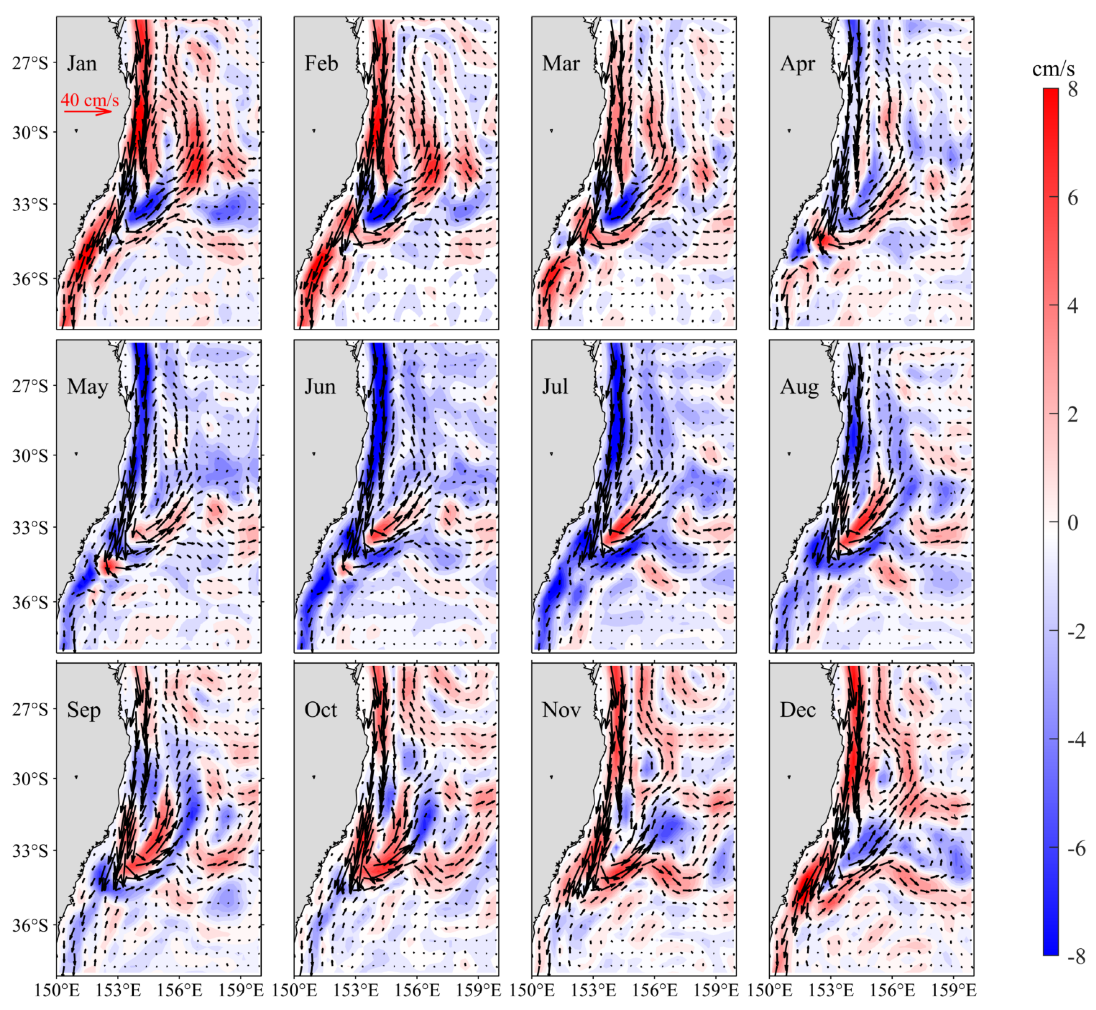
To better understand the dynamic processes of eddy–mean flow interaction in the EAC region, we also analyze the seasonal variation of the 180-day low-passed EAC (Figure 10). The EAC is strong in the coastal region, and the northward EAC countercurrent is formed at about 33° S. Due to the existence of countercurrent, the anticyclonic recirculation is formed in the offshore sea, further promoting the generation of eddies in the offshore sea. It can be seen that the anticyclonic recirculation is strongest in January, and the southern end of the recirculation can reach to about 35° S. From February, the anticyclonic recirculation begins to weaken, and it almost disappears in June, accompanied by a less sharp angle of retroflection. From July, the anticyclonic recirculation gradually increases as the season progresses, reaching its peak in January in the following year, completing the annual cycle. In addition, it is clear that the southward mean EAC shows an annual cycle, which is stronger in austral summer and weaker in austral winter. To visualize the variation more intuitively, we also calculated the time series of the EAC velocity averaged in the upper 500 m layer as a function of months, which is shown in Figure 9 (green line). The result reveals that the spatial averaged EAC velocity reaches its peak in January (12.9 cm/s) and its trough in June (7.9 cm/s), which is the same as the seasonal BTR variation (red solid line). In summary, barotropic instability of the background mean circulation is associated with the EAC strength in this region. In austral summer, the larger EAC velocity promotes a stronger anticyclonic recirculation around the EAC separation latitude and favors the barotropic instability of the mean flow, and vice versa in austral winter.

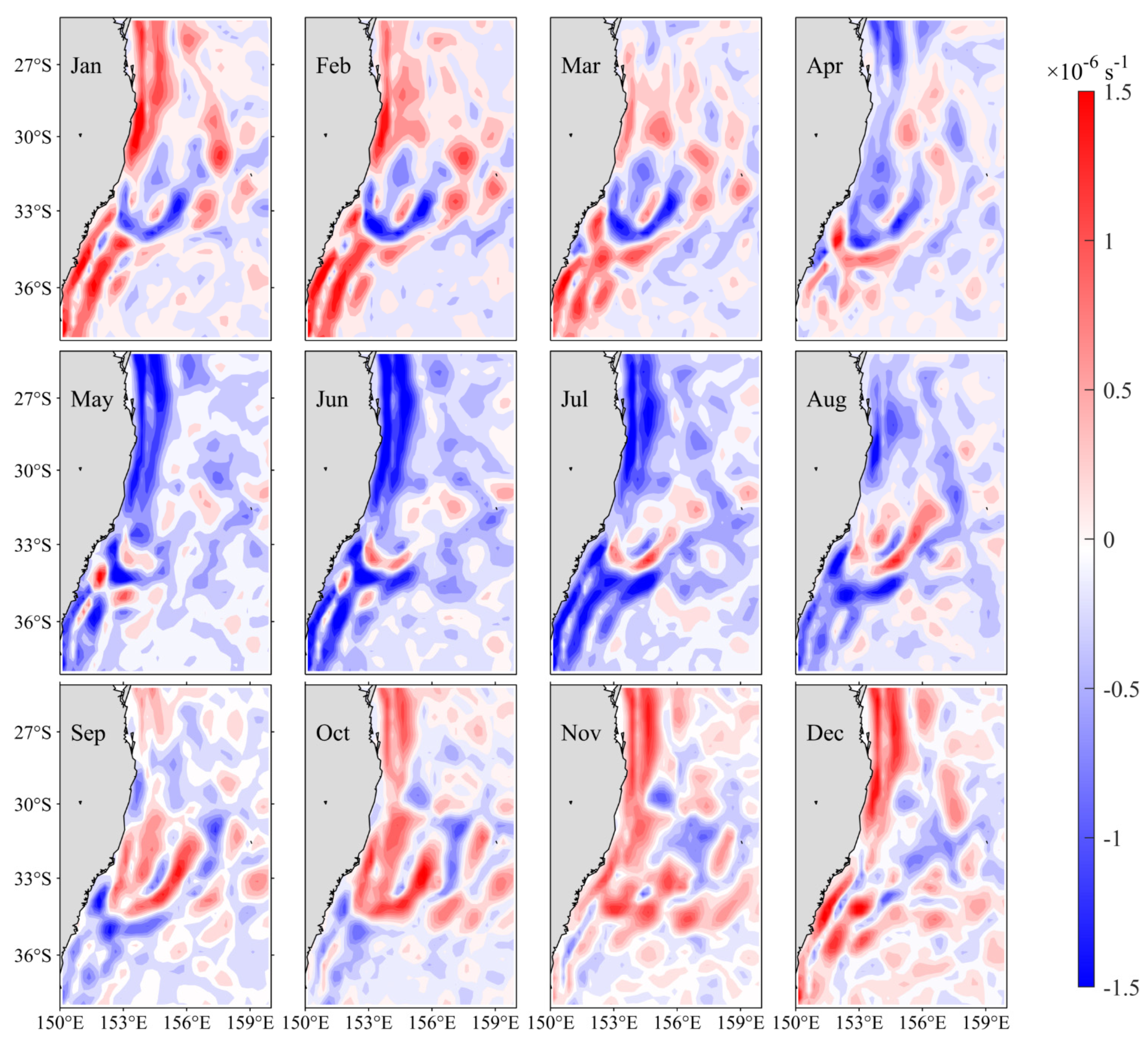
The occurrence of barotropic instability usually requires strong horizontal shear of the background mean flow. To further confirm our above conclusion, we calculated the lateral rate of strain (refer to as LRS in the following) as follows (Rocha et al., 2016 [21]), which can quantitatively characterize the magnitude of horizontal velocity shear:

$$\mathrm{S}=\sqrt{{\left(\frac{\partial \tilde{u}}{\partial x}-\frac{\partial \tilde{v}}{\partial y}\right)}^2+{\left(\frac{\partial \tilde{v}}{\partial x}+\frac{\partial \tilde{u}}{\partial y}\right)}^2}$$

(6)

where, $\tilde{u}$ and $\tilde{v}$ represent the 180-day low-pass filtering velocities. Figure 11 shows the monthly LRS anomaly distributions in the upper 500 m layer, which have subtracted the annual mean value. In general, the seasonal evolution of LRS is similar to the seasonal variation of the EAC mean flow, which further validates our above conclusion.

In summary, the seasonal variation of EKE along the EAC and the related dynamic processes are examined in this paper. Our result reveals that the evolution of EKE is mainly controlled by the barotrophic instability of the EAC. In austral summer, the stronger southward-extending EAC promotes the formation of the anticyclonic recirculation, which favors the barotropic instability of the mean flow, elevating the regional EKE level. All these processes are reversed in austral winter. Meanwhile, it can be seen in Figure 10 that the EAC separation latitude also shifts north–south with seasons, which agrees well with the previous study (Oke et al., 2019 [22]). Extending the previous study, our result reveals that the barotropic instability is mainly controlled by the strength of the EAC. At the same time, it can be noticed that the EKE from ECCO2 state estimate is a litter weaker than that from AVISO data, which may relate to the eddy-permitting resolution (0.25° × 0.25°) of the ECCO2 state estimate. Thus, a high-resolution ocean state estimate is needed in the future to more accurately capture the magnitude of the EKE variations.

Based on global eddy databases (Chelton et al., 2007 [23]; Chelton et al., 2011 [24], Everett et al., 2012 [15]) emphasized the vital roles of eddies in this region, known as the “Eddy Avenue”, whose eddy transport can explain 46% of the total southward volume transport (Cetina-Heredia et al., 2014 [7]). Considering the wrapping capacity of mesoscale eddies, more in situ observations and high-resolution modeling studies are needed to understand the impact of eddy-shedding activities on inter-basin heat/fresh water transport and their impact on ecologies in the Southern Ocean.

References

- Bowen, M.M.; Sutton, P.J.H.; Roemmich, D. Wind-driven and steric fluctuations of sea surface height in the southwest Pacific. Geophys. Res. Lett. 2006, 33, L14617. [Google Scholar] [CrossRef]
- Speich, S.; Blanke, B.; de Vries, P.; Drijfhout, S.; Döös, K.; Ganachaud, A.; Marsh, R. Tasman leakage: A new route in the global ocean conveyor belt. Geophys. Res. Lett. 2002, 29, 55-1–55-4. [Google Scholar] [CrossRef] [Green Version]
- Ridgway, K.R.; Godfrey, J.S. Seasonal cycle of the East Australian Current. J. Geophys. Res. Oceans 1997, 102, 22921–22936. [Google Scholar] [CrossRef] [Green Version]
- Imawaki, S.; Bower, A.S.; Beal, L.; Qiu, B. Western Boundary Currents. In Ocean Circulation and Climate—A 21st Century Perspective, 2nd ed.; Siedler, G., Griffies, S.M., Gould, W.J., Church, J., Eds.; Academic Press: Cambridge, MA, USA, 2013; pp. 305–338. [Google Scholar]
- Ridgway, K.R.; Dunn, J.R. Mesoscale structure of the mean East Australian Current System and its relationship with topography. Prog. Oceanogr. 2003, 56, 189–222. [Google Scholar] [CrossRef]
- Tilburg, C.E.; Hurlburt, H.E.; O’Brien, J.J.; Shriver, J.F. The Dynamics of the East Australian Current System: The Tasman Front, the East Auckland Current, and the East Cape Current. J. Phys. Oceanogr. 2001, 31, 2917–2943. [Google Scholar] [CrossRef]
- Cetina-Heredia, P.; Roughan, M.; van Sebille, E.; Coleman, M.A. Long-term trends in the East Australian Current separation latitude and eddy driven transport. J. Geophys. Res. Oceans 2014, 119, 4351–4366. [Google Scholar] [CrossRef] [Green Version]
- Schaeffer, A.; Roughan, M.; Wood, J.E. Observed bottom boundary layer transport and uplift on the continental shelf adjacent to a western boundary current. J. Geophys. Res. Oceans 2014, 119, 4922–4939. [Google Scholar] [CrossRef]
- Qiu, B.; Chen, S. Seasonal Modulations in the Eddy Field of the South Pacific Ocean. J. Phys. Oceanogr. 2004, 34, 1515–1527. [Google Scholar] [CrossRef]
- Ypma, S.L.; van Sebille, E.; Kiss, A.E.; Spence, P. The separation of the East Australian Current: A Lagrangian approach to potential vorticity and upstream control. J. Geophys. Res. Oceans 2016, 121, 758–774. [Google Scholar] [CrossRef]
- Zilberman, N.V.; Roemmich, D.H.; Gille, S.T.; Gilson, J. Estimating the Velocity and Transport of Western Boundary Current Systems: A Case Study of the East Australian Current near Brisbane. J. Atmos. Ocean. Technol. 2018, 35, 1313–1329. [Google Scholar] [CrossRef]
- Mata, M.M.; Wijffels, S.E.; Church, J.A.; Tomczak, M. Eddy shedding and energy conversions in the East Australian Current. J. Geophys. Res. 2006, 111, C09034. [Google Scholar] [CrossRef] [Green Version]
- Bowen, M.M.; Wilkin, J.L.; Emery, W.J. Variability and forcing of the East Australian Current. J. Geophys. Res. Oceans 2005, 110, C03019. [Google Scholar] [CrossRef] [Green Version]
- Wilkin, J.L.; Zhang, W.G. Modes of mesoscale sea surface height and temperature variability in the East Australian Current. J. Geophys. Res. 2007, 112, C01013. [Google Scholar] [CrossRef] [Green Version]
- Everett, J.D.; Baird, M.E.; Oke, P.R.; Suthers, I.M. An avenue of eddies: Quantifying the biophysical properties of mesoscale eddies in the Tasman Sea. Geophys. Res. Lett. 2012, 39, 16608. [Google Scholar] [CrossRef] [Green Version]
- van Sebille, E.; England, M.H.; Zika, J.D.; Sloyan, B.M. Tasman leakage in a fine-resolution ocean model. Geophys. Res. Lett. 2012, 39, L06601. [Google Scholar] [CrossRef] [Green Version]
- Travis, S.; Qiu, B. Decadal variability in the South Pacific Subtropical Countercurrent and regional mesoscale eddy variability. J. Phys. Oceanogr. 2017, 47, 499–512. [Google Scholar] [CrossRef] [Green Version]
- Menemenlis, D.; Fukumori, I.; Lee, T. Using Green’s functions to calibrate an ocean general circulation model. Mon. Weather Rev. 2005, 133, 1224–1240. [Google Scholar] [CrossRef] [Green Version]
- Chen, X.; Qiu, B.; Chen, S.; Qi, Y.; Du, Y. Seasonal eddy kinetic energy modulations along the North Equatorial Countercurrent in the western Pacific. J. Geophys. Res. Ocean. 2015, 120, 6351–6362. [Google Scholar] [CrossRef] [Green Version]
- Yang, C.; Chen, X.; Cheng, X.; Qiu, B. Annual versus semi-annual eddy kinetic energy variability in the Celebes Sea. J. Oceanogr. 2020, 76, 401–418. [Google Scholar] [CrossRef]
- Rocha, C.B.; Gille, S.T.; Chereskin, T.K.; Menemenlis, D. Seasonality of submesoscale dynamics in the Kuroshio Extension. Geophys. Res. Lett. 2016, 43, 11304–11311. [Google Scholar] [CrossRef]
- Oke, P.R.; Roughan, M.; Cetina-Heredia, P.; Pilo, G.S.; Ridgway, K.R.; Rykova, T.; Archer, M.R.; Coleman, R.C.; Kerry, C.G.; Rocha, C.; et al. Revisiting the circulation of the East Australian Current: Its path, separation, and eddy field. Prog. Oceanogr. 2019, 176, 102139. [Google Scholar] [CrossRef]
- Chelton, D.B.; Schlax, M.G.; Samelson, R.M.; de Szoeke, R.A. Global observations of large oceanic eddies. Geophys. Res. Lett. 2007, 34, L15606. [Google Scholar] [CrossRef]
- Chelton, D.B.; Schlax, M.G.; Samelson, R.M. Global observations of nonlinear mesoscale eddies. Prog. Oceanogr. 2011, 91, 167–216. [Google Scholar] [CrossRef]
Figure 1.
Climatology absolute dynamic topography (ADT, colors) and surface velocities (black arrows) in the western Pacific from (a) AVISO data and (b) ECCO2 state estimate outputs. Both results are averaged between January 1993 and October 2019.
Figure 2.
Climatology eddy kinetic energy (EKE) distributions calculated from surface velocities of (a) AVISO and (b) ECCO2. (c) shows the distribution of AVISO EKE minus ECCO2 EKE. Red box indicates the area in which EKE time series and budget are calculated.
Figure 3.
Surface EKE time series averaged in 150−160° E, 25−38° S as a function of months. EKE is calculated by using surface velocities of AVISO (red line) and ECCO2 (black line).
Figure 4.
Variance-preserved power spectra as a function of periods of the sea surface height from AVISO (red line) and ECCO2 (blue line) data in the area of 150−160° E, 25−38° S.
Figure 5.
Blue line: EKE averaged in 150–160° E,25–38° S as a function of depth from the ECCO2; the EKE level has been normalized by its surface value: 〈E(t, z)〉/〈E(t, 0)〉. Red line: EKE coherence level as a function of depth with respect to the surface EKE values; see Equation (3) for the definition of coherence level.
Figure 6.
Monthly mean climatological EKE distributions in the upper 500 m layer. Here EKE is calculated from the 60–180-day bandpass filtered velocity data from the ECCO2 (1992–2019).
Figure 7.
Monthly mean climatological barotropic conversion rate (BTR) distribution in the upper 500 m from the ECCO2. See Equation (4) for the definition of BTR.
Figure 8.
Monthly mean climatological baroclinic conversion rate (BCR) distribution averaged in the upper 500 m layer. See Equation (5) for the definition of BCR.
Figure 9.
Monthly mean climatological eddy kinetic energy (EKE, black line), barotropic conversion rate (BTR, red solid line), baroclinic conversion rate (BCR, red dash line) in the upper 500 m averaged over (150–160° E, 25–38° S). Green line denotes the monthly mean climatological variations of the southward velocity in the upper 500 m averaged over (150–155° E, 25–38° S), which has been 180-day low-pass filtered.
Figure 10.
Monthly mean climatological background current distributions averaged in the upper 500 m layer, and color indicates velocity magnitude anomalies which have subtracted the annual mean value. Here velocities are based on the 180-day low-pass filtered ECCO2 outputs.
Figure 11.
Monthly mean climatological lateral rate of strain (LRS) anomalies distributions averaged in the upper 500 m layer, which have subtracted the annual mean value. Here velocities are based on the 180-day low-pass filtered ECCO2 outputs.
Publisher’s Note: MDPI stays neutral with regard to jurisdictional claims in published maps and institutional affiliations. |
© 2022 by the authors. Licensee MDPI, Basel, Switzerland. This article is an open access article distributed under the terms and conditions of the Creative Commons Attribution (CC BY) license (https://creativecommons.org/licenses/by/4.0/).
Share and Cite
MDPI and ACS Style
Xu, Z.; Yang, C.; Chen, X.; Qi, Y. Seasonal Variation of Intra-Seasonal Eddy Kinetic Energy along the East Australian Current. Water 2022, 14, 3725. https://doi.org/10.3390/w14223725
AMA Style
Xu Z, Yang C, Chen X, Qi Y. Seasonal Variation of Intra-Seasonal Eddy Kinetic Energy along the East Australian Current. Water. 2022; 14(22):3725. https://doi.org/10.3390/w14223725
Chicago/Turabian StyleXu, Zhipeng, Chengcheng Yang, Xiao Chen, and Yiquan Qi. 2022. "Seasonal Variation of Intra-Seasonal Eddy Kinetic Energy along the East Australian Current" Water 14, no. 22: 3725. https://doi.org/10.3390/w14223725
Note that from the first issue of 2016, this journal uses article numbers instead of page numbers. See further details here.