Geospatial Technologies Used in the Management of Water Resources in West of Romania

Abstract

Stability in time of major and important objectives is vital and can be achieved by 3D scanners which follow changes in time with construction, respective of the natural or artificial hydrotechnical dams and the obtaining of 3D data in real time with the possibility of evaluating and making quick decisions. This scientific paper approaches a research topic of great importance and actuality in the field of Civil Engineering, Hydrotechnics, and Geomatics using the 3D scanning technologies for the hydrotechnical arrangements (Topolovăţu Mic, Coșteiu and Sânmartinu Maghiar) and hydroameliorative (Cruceni Pumping Station). In Romania, data collection was carried out for the first time using the mobile scanning technology (MMS), “Backpack” type, namely, Leica Pegasus Backpack. Data collection using terrestrial laser scanning technology (Terrestrial Laser Scanning) was carried out with the Leica C10 equipment. The processing of point clouds was carried out using the Inertial Explorer program, and the processing of point clouds was carried out with the Cyclone program. The collection of ground checkpoints used for checking, correcting, and analyzing point clouds was carried out using the GPS Leica GS08 equipment. Compared with traditional methods using classical measuring instruments, precise data was obtained (with an error of 2–4 cm) through 3D laser scanning technology in a short time and with multiple possibilities of processing and visualizing point clouds.

1. Introduction

The evolution of technologies in the last half of the twenty-first century has led to huge progress in electronics, IT, and graphics (digital 3D models), making possible the development of laser scanning technology, both terrestrial and aerial. Thus, the possibility of processing the dense clouds of points in an efficient and cost-effective way facilitated a multitude of applications regarding the acquisition of 3D data in areas such as topography, environmental protection [1,2], the completion and conservation of cultural heritage, forest resources, etc. [3,4]. The first 3D scanning technology was created in the 1960s.

In modern engineering [5], the term “laser scanning” is used to describe two meanings closely related to each other but still separated. The first sense, more generally, is the controlled deviation of laser beams, visible or invisible [6]. The second direction, more specifically, is the controlled direction of the laser beams followed by the measurement of the distance in each direction indicator. This method, often called 3D scanning of an object or 3D laser scanning, is used to quickly capture shapes of objects, buildings, and landscapes.

The 3D laser scanning market, including hardware, software, and services, is quite dynamic, with major segments facing rapid product innovation [7]. Laser scanning systems have gone through a major evolution over the past decade. After the initial discovery of Airborne Laser Scanners (ALS), other types of laser scanning systems [8] appeared, namely terrestrial laser scanners (TLS) and Mobile Mapping Systems (MMS).

Many applications require 3D object data, and examples can be found in civil and industrial engineering, construction [9] and road maintenance, urban planning, environmental analysis [2], and precision forestry. LiDAR (Light Detection and Ranging) was widely used over the years to scan objects or map the environment in 3D to support these applications.

The types of ALS, TLS, and MMS systems each have their own applications, advantages, and disadvantages. A TLS may be suitable for the field, but it may be inappropriate due to the limited number of points and the requirement of excessive redundancy of data for the successful recording of the scan. Therefore, the growing need for modelling and monitoring of objects challenges the industry to develop new 3D data collection tools which are even more complete, accurate, and efficient [10].

Terrestrial Laser Scanning (TLS) uses the same principles as ALS, by allowing datasets to be collected far above this traditional topography [11].

The laser scanner can be described as a fully motorized station which automatically measures all points in its horizontal and vertical field [12].

Laser scanning and its synonyms LADAR (Laser Distance and Ranging) or LiDAR have become a major technology for the three-dimensional geometric capture of complex structure data [13,14]. Unlike classic photogrammetry, which requires a minimum of two images and provides image coordinates that must be scaled and transformed to generate 3D information, laser scanning directly generates a metric 3D information. Each point of this point cloud has three-dimensional coordinates [15] and has accuracy up to a few millimeters. In addition, the intensities of the received signals provide valuable indicators for post-processing.

Currently, LiDAR technology is used in more and more fields [16], and information about LiDAR technology dates back long before the discovery of the laser. For example, in 1930, the first attempt to measure the density of air in the upper part of the atmosphere appears. In 1960, the year of the discovery of the laser, we proceeded to the development of modern LiDAR systems, an evolution that is constantly growing.

The use of IMU for navigation has been largely limited to aviation and the maritime industry due to costs and sizes [17]. In recent decades, the IMU has become less expensive with the introduction of a micro-machined electromechanical technologies MEMS (Micro-machined electromechanical Systems), which allows many consumer products, such as mobile phones, cameras, and game consoles, to include an IMU [17]. Recent progress in computer processing has allowed image processing algorithms to be disseminated in real-time, even on consumer products, and together with the help of less expensive IMU, vision-assisted inertia navigation has become very important in the research field [18,19].

IMU measures acceleration and angular velocity, and measurements can be integrated over time to achieve a position and orientation.

The noise inherent in IMU measurements are also included in the integration and will cause position and orientation estimates to distance from the true value. An IMU can be taken with a very high sampling frequency, in which rapid movements are felt very well. An image does not represent a single moment of time but the scene in time. Images on a camera must be processed through an image processing algorithm to obtain a position. Image processing takes time and limits the frequency at which the position can be obtained from a camera.

The purpose of this paper is to carry out a scientific research using modern techniques and methods of scanning and measuring heritage objectives (the hydrotechnical nodes from Topolovăţu Mic and Coșteiu, the lock from Sânmartinu Maghiar as well as the Cruceni pumping station) with modern technologies in order to preserve in time these objectives of national and international interest, thus offering Romania and Serbia, through the IPA program, the ability to carry out the project of “rehabilitation of the infrastructure of the Bega Navigable Canal”, which has a value of 13.878 million euros (VAT included). The partners of this project are: Banat Water Basin Administration (project leader-Romania), Timis County Council and, from Serbia, the Provincial Secretariat for Interregional Cooperation and VDP Vode Vojvodine.

2. Materials and Methods

2.1. Methodology

The research explores the many representations and digital tools of the field to create digital environments using Leica 1200 and Leica GS08 GPS equipment, terrestrial laser (TLS), Leica ScanStation C10, Dorna (UAV) Phantom 4 Pro, and an ultramodern LiDAR mobile MMS (Mobile Mapping System) piece of scanning equipment, the Pegasus Backpack model, which offers unique mobile mapping solutions for fast reality capture and combines five cameras providing a 360-degree and two-degree panoramic view sensors which are based on LiDAR technology, Velodyne type (VLP16) [20], for measuring the laser distance, managing to determine 600 thousand points per second, at a maximum distance of 60–70 m left-right (300 thousand points/s for SA—vertical scanning and 300 thousand points/s for HS-horizontal scanning) (Figure 1).

In the current research, the Leica Pegasus Backpack scan was chosen because the differences between this scan (MMS) [21] and the GNSS measurements are about 2–3 cm at an absolute level, and the relative results are even better (in the order of millimeters, 13–20 mm). With such equipment, in addition to speed and accuracy in obtaining 3D data, one may also discuss a cost saving of almost 50%. The advantage of 3D scanning is that, at the time of scanning, the entire area will be captured, so that any forgotten detail may be obtained later, without the need for another exit into the field, for completion. Thus, UAV and MMS data can be combined with existing research technologies such as TPS, GPS and TLS, providing a more complex set of information.

By using SLAM (Simultaneous Localization and Mapping) technology, ARTK (Advance Real Time Kinematic) technology to solve ambiguities (minimum 5 satellites from the same constellation, optimal would be 7 or more), and high-precision IMU (Inertial Measurament Unit), the Leica Pegasus Backpack equipment ensures precise positioning together with GNSS technology [22] incorporated into the equipment and of Kalman filter. The final results are 3D point clouds (3D Point Cloud), orthophotoplane, a digital surface model (DSM) and a digital elevation model (DEM), 3D model, 3D polygons and polylines, GIS data [23], as well as 3D/2D situation plans that can also be made and overlapped on clouds of points collected from the field.

2.1.1. GNSS Technology

The GNSS campaign was carried out for all the locations taken in the study, but for the current paper, only the data for the Topolovăţu Mic hydrotechnical node will be presented. Rinex data recording was carried out using double frequency receivers Leica 1200 and Leica GS08 and GS08 plus.

The 1200 series and the GS08 series were used either as a reference station or as a Rover for both static measurements and kinematic measurements (RTK).

In the paper, for Rinex data recording, the static method has been used, and the data acquisition was carried out at 5 s by activation of the Long Raw Observation function. The measuring engine used is SmartTrack type which acquires satellites in seconds. The antennas used are of double frequency type: AX1202GG and ATX1230GG with SmartTrack, supporting GLONASS, GPS, and GALILEO signals. The raw data obtained was exported from the Leica 1200 GPS control using the Leica Geo Office Combined (RAW DATA) program. The reference system was WGS 84 (World Geodetic System).

For GS08 receivers, Rinnex data downloading was performed directly from the controller to USB. In order to achieve the post-processing of the data obtained from the field (by stationing with the GPS equipment on the concrete terminals) the Rinnex data was also acquired from the Permanent Stations, every 5 s, and together with the data acquired in the field, the post-processing and obtaining the WGS 1984 coordinates of the stationed terminals, have been carried out.

The transformation of the raw data (RAW DATA) from the ETRS89 system into the 1970 Stereographic projection system (which represents the official cartographic projection of Romania) was carried out within the paper with the TransDatRO program and, after that, passed to report the points in AutoCAD through the TopoLT program and their comparison with GNSS RTK values obtained from field readings.

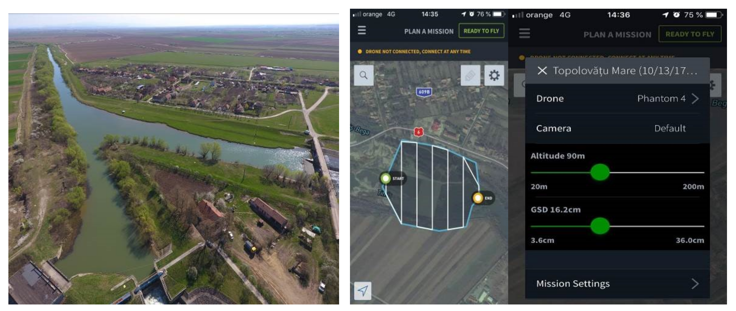
2.1.2. UAV Technology

For the acquisition of aerial data [24], during the course of the research carried out, a Phantom 4 Pro Drone was used.

In the present work, the flight was carried out at a relative altitude of 90 m, over four parallel strips running in the North-South direction and two boarding lanes (Figure 2). The flight data was uploaded to the UAV using a wired connection, through an Iphone SE phone, which allows receiving and sending information on position, orientation, height, and speed during the flight.

2.1.3. TLS Technology

In order to restore some patrimony monuments, two Hydrotechnical Nodes (Coşteiu and Topolovăţu Mic, Timiș County, Romania), two locks (Sânmihaiu Român and Sânmartinu Maghiar, Timiş County, Romania) and a Pumping Station in Cruceni, Timiş County were used; knowing the geometry of the object represents the most important part.

A complex analysis of constructions can usually be done by making a simple drawing, or a spatial representation of the object, which is based on a limited number of shapes, as well as lines, points, or polygons.

In this study, a TLS laser scanner from Leica, the C10 model, was used, which has an acquisition range from 0.6 m up to 300 m, and which also has the possibility to overtake images through an integrated camera, making 260 RAW images from each station.

Between 2017–2019, a total of eight scans were performed to cover the studied surface, namely: 2 TLS scans at NH Coșteiu; 3 TLS scans at Topolovăţu Mic; 1 TLS scan at NH Sânmihaiu Român; 1 TLS scan at Sânmartinu Maghiar, and 1 TLS scan at Cruceni Pumping Station, with the possibility to choose the size of the GRID, the acquisition speed being 50,000 points per second.

The final coordinates resulted from the post-processing of the raw data and the acquisition of RINNEX data from the GNSS permanent stations.

The stationary time for each scan was between 25–75 min, in the case of scans performed within the current scientific paper, at a GRID of 2 cm of scanning. During this time of stationary, the Leica C10 scanner (TLS) used for scanning analyzes the maximum distance set for scanning and, depending on the size of the GRID, the stationary time will be determined.

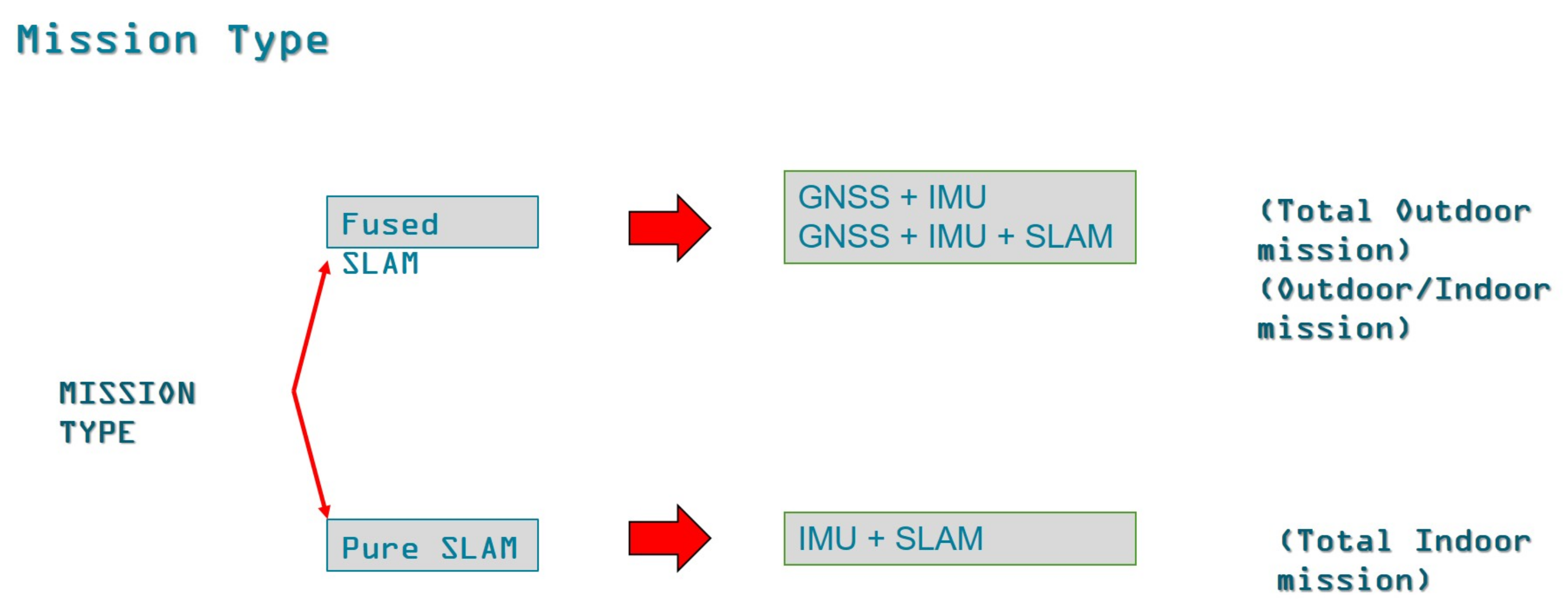
2.1.4. MMS Technology

Leica Pegasus Backpack [20] is a platform with reality capture sensors, with a highly ergonomic design, combining five cameras that offer a fully calibrated 360-degree view and two LiDAR sensors (VLP-16) with an ultra-light carbon fiber chassis, allows obtaining LiDAR points, both inside (PURE SLAM method) and inside or outside (FUSED SLAM method), at a level of precision considered to be authoritative and professional (Figure 3).

LiDAR Data Acquisition Using MMS

For the acquisition of MMS data, the Hydrotechnical Node from Coșteiu and the two Locks have been scanned: Sânmihaiu Român and Sânmartinu Maghiar, as well as a scan at the Cruceni Pumps in the county Timis, the FUSED SLAM method being used for all the locations (Figure 4).

• Planning the LiDAR data acquisition mission: preparing the street lanes for the missions performed outside or the route on which it will have to be followed or, in case of inside scanning, viewing the interior and creating space for turns and walks, opening and fixing the doors. Planning for the three objectives was done using the Google Earth [25] outdoor program.
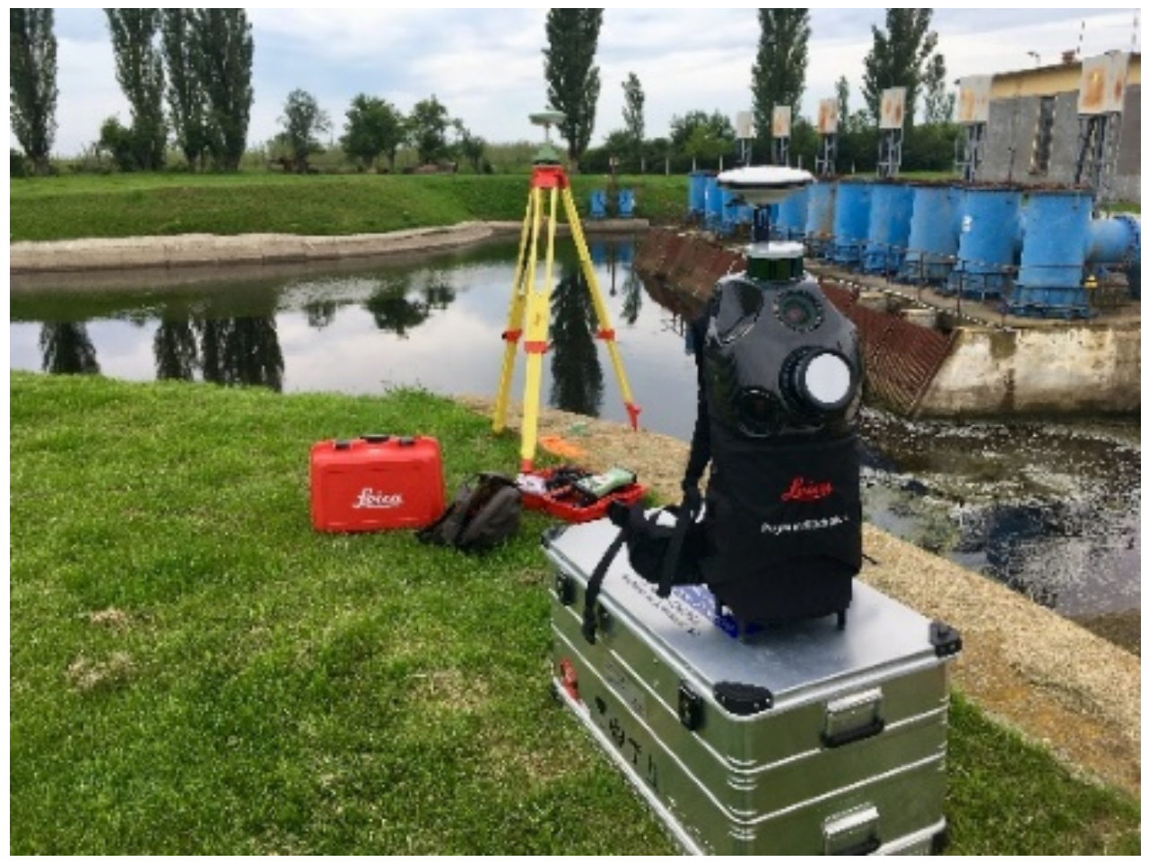
• Initialization of the equipment: in order to obtain data with high accuracy, the initialization has been done near the scanned objectives, in open air area, not covered by obstacles (trees, buildings). Initialisation consists of two steps (Figure 5):
  • STATIC initialization, for a period of 5 min, during which the backpack will stand still for 15–20 min.
  • min in case the ALMANAC will have to be updated, Almanach update needed when travelling > 200 km from last project site.
  • DYNAMIC initialization, with a duration of 3–5 min, during which the backpack is worn on the back, making a quadrilateral walking with it in the back, and, at the end, a walk on the diagonals of the quadrilateral until the INS GOOD message appears, and the INS_GNSS will have a value below 1; usually, the indicated value is 0.1–0.2.

Placing the Master GNSS Station and Collection of GCP Control Points

For the acquisition of LiDAR [26] data for the objectives pursued in this paper, the FUSED SLAM method was used, a method to which, in addition to the scanning backpack itself, we also need the placement of a Master GNSS station for field acquisition and Rinex data, an acquisition that was set to an interval of 1 s for the post-processing of the measurement trajectory as opposed to the static measurements for the thickening of the geodetic network that was set to a Rinex data acquisition at 5 s.

It is mandatory to have GNSS data at 1Hz or higher from the maximum location distance of the Master station, which must not exceed a maximum of 15 km from the position of the Leica Pegasus backpack. It may also be used the GNSS reference stations located at the Romania Offices of Cadastre and Real Estate Advertising, for a fee (3 EUROS/hour/reference station). In carrying out the post-processing for this work, a Master station was used, and the Leica GS 08 plus model was used, which was mounted on a tripod for each of the measurements in order to record the RINNEX data (Figure 6).

A more precise transformation was achieved with the Leica Infinity program. But the best solution was to record RTK data directly in the 1984 WGS system without turning it directly into the field or office (

Table 1. Master station coordinates for targets scanned in the WGS 1984 system.

No. Crt.	Master Station	Type	B [m]	L [m]	He [m]
1	H NCoşteiu	FENO Terminal	45°44′10.90829″ N	21°51′07.31158″ E	157.481
2	Cruceni pumps	FENO Terminal	45°27′05.562528″ N	20°53′15.953888″ E	120.995
3	HN Sânmartinu Maghiar	Metal bolt	45°39′26.63270″ N	20°55′28.31293″ E	126.516

).

For the correct collection of Rinex data, the Master GNSS station (for all scanned objectives) was started 10 min before the initialization of the backpack (Leica Pegasus Backpack) and was turned off 10 min later after completing the collection of LiDAR data. For each of these scans, GCP checkpoints (

Table 2. GCP ground checkpoints collected in the field.

Objective	Name	X (m)	Y (m)	Z (m)
HN Coşteiu	Master_SR1	475,565.920	255,206.307	114.399
	1RTK	475,558.675	255,259.001	114.607
	2RTK	475,591.581	255,275.722	116.604
	3RTK	475,610.997	255,258.163	116.986
	4RTK	475,596.074	255,240.448	116.822
	4RTK	475,620.283	255,221.991	116.501
HN Sânmihaiu Român	Master_SR1	475,209.986	196,699.310	84.695
	GPS1	475,180.393	196,683.443	86.942
	GPS2	475,178.302	196,678.649	86.940
	GPS12	475,267.737	196,623.461	86.615
	GPS13	475,266.853	196,621.210	86.610
	GPS14	475,213.282	196,711.086	84.727
	GPS20	475,193.586	196,719.979	84.712
Cruceni pumping station	Master_SR1	447,352.270	178,587.621	77.771
	GPS1	447,343.822	178,583.799	77.941
	GPS2	447,343.710	178,593.625	77.576
	GPS3	447,330.955	178,596.606	77.627
	GPS4	447,349.065	178,611.745	77.509
H NSânmartinu Maghiar	Master_SM1	470,063.192	182,627.374	83.394
	GPSM1	470,066.158	182,631.739	83.382
	GPSM2	470,100.617	182,696.315	83.356
	GPSM13	470,078.430	182,624.035	83.391

) were determined directly in the field on the ground with the GPS equipment from Leica GS 08, and points that were used to check and realign the clouds of LiDAR points were collected with the Leica Pegasus Backpack equipment. The checkpoints were also imported into the Pegasus Manager to verify the quality of the recorded data and to verify the trajectory of the scanned objectives (Figure 7).

2.2. Description of the Hydrotechnical and Hydro-Ameliorative Arrangements under Study

From an administrative point of view, Banat is located in the Western Development Region of Romania, occupying entirely the administrative districts of Timiș county (47.46%), Caras-Severin (46.47%), and smaller parts of the counties: Arad (2.89%), Gorj (0.90%) and Mehedinti (2.29%). This hydrographic area covers an area of 18,272 km² (7.7% of the total area of Romania) and consists of several hydrographic basins, whose main watercourses have a cross-border character. These basins are represented by the Bega-Timiș-Caraş hydrographic basin [27], the Nera-Cerna hydrographic basin, the Danube hydrographic basin between Baziaș and the interfluve with the Cerna river, and the Aranca hydrographic basin [28].

The hydrographic network [28,29,30] from the Banat hydrographic area has a length of 6297 km and consists of 10 watercourses (Aranca, Bega Veche, Bega, Timiș, Bârzava, Moravița, Caraș, Nera, Dunărea and Cerna) and their tributaries crossing the state border with Serbia and the Danube tributaries between Baziaș and the Cerna River (

Table 3. Hydrographic network in the Banat hydrographic area (http://www.rowater.ro (accessed on 14 May 2021).

Hydrographic Basin	Basin Area (km2)	Length of the Network (km)	Main Course Length (km)
Aranca	1080	328	114
Old Bega	2108	527	107
Bega	2362	892	170
Timiş	5673	1907	244
Bârzava	1202	355	127
Moraviţa	387	172	47
Caraş	1280	502	79
Nera	1380	574	124
Tributaries of the Danube
(between Buziaş and Cerna)	1091	530	123
Cerna	1360	524	79

).

The Bega River [27], the second largest river (after the Timiş River) in the analyzed area, has an area of 2362 km2, a length of 170 km to the Romanian border and a hydrographic network density of 0.38 km/km2 [31]. In the eighteenth century, this river was channeled on the lower course, at 114 km, between the localities of Timișoara (Romania) and Titel (Serbia), being the first navigable canal in Romania and, by its completion, Timisoara became the first Romanian city with a navigable canal and an operational port.

2.2.1. Topolovăţu Mic Hydrotechnical Node

The Topolovăţu Mic hydrotechnical node is part of the hydrotechnical planning: “The Double Timiș-Bega Connection”, which was conceived by the Dutch engineer Maximilian Emmanuel de Fremaut and built in 1758 [27,32]. In order to defend the municipality of Timisoara from high waters, the dam from Topolovăţ controls, on Beghei, a maximum flow of 40 m³/s, and the extra flow is discharged in Timiș through a channel of 5.5 km long. Also, in order to ensure the level of navigation on the Bega Canal through the dam from Coșteiu, the Bega Canal from the Timiș River is fed through a channel of 10 km with the necessary flow [27,29].

The Timis—Bega interconnection is an anthropogenic [33] and natural system of watercourses. The spillway threshold (dam) at Coșteiu is located downstream of Lugoj. The spillway threshold was built in the eighteenth century to divert the water from Timis to the Bega through the 10 km long Timiș-Bega supply Canal to ensure the water supply of the Bega Canal and implicitly of the city of Timisoara.

In the over 200 years of existence, the arrangement has suffered various damages and restorations, and in 1998 the entire hydrotechnical node was damaged as a result of the floods, appearing a series of infiltrations, erosions, and breaches in the body of the dam.

The Topolovăţu Hydrotechnical Node has a great importance for the Banat plain area because it supplies water with almost constant level to the Bega Canal, thus decreasing the probability that the Timisoara municipality will be affected by drought, being favorable to navigation on the Bega Canal, which can be carried out all year round, and the floods on this river can be controlled; thus, the localities downstream of the dam are protected to some extent from unpredictable floods [27].

2.2.2. Coșteiu Hydrotechnical Node

It aims to make connections between the Timiş River and the Bega Canal since 1758. The hydrotechnical node was built in 1758 with the purpose of directing the waters of the Timiș River into the Bega Canal in times of drought for the latter to have a constant flow. This regulates the flow of the Bega Canal, which ensures the necessary drinking water (for a part of Timisoara) as well as the flow required for navigation. At the same time, the hydrotechnical node from Coșteiu performs the function of defense against floods.

It is a hydrotechnical derivation system located at the branching of the Timiș-Bega discharge channel. From the administrative point of view, N.H. Coşteiu is located in Timiș County, Coşteiu Commune.

The Timiş–Bega interconnection is a double connection consisting of two channels connecting the Timiş River and the Bega River [33,34,35] via a discharge channel (Figure 8).

The Coșteiu Hydrotechnical Node is one of the five hydrotechnical nodes administered by the Banat Water Directorate [36]. It is the only hydrotechnical system located on the Timiș River, the other four hydrotechnical nodes being built on the Bega.

The dam has a canopy length of 130 m and a height of 10.5 m. The Timiș dam is a spillway dam, with a wide threshold of rocks in wooden houses filled with raw stone. In 1998 the entire hydrotechnical node was damaged by floods [37].

In terms of importance, the Coșteiu Hydrotechnical Node has a particularly high importance for the Banat plain area. First of all, the hydrotechnical works in Coștei supply the Bega Canal with water, thus decreasing the probability that Timisoara municipality to be affected by drought. At the same time, the supplementation of the water flow from Timiș to the Bega is also favorable for navigation on the Bega Canal, which can take place throughout the year. Through the spillway dam built on The Timis, the floods on this river can be controlled so that the localities downstream of the dam are protected to some extent from unpredicted floods. The fact that the dam provides a constant level of water upstream facilitates the water supply to the municipality of Lugoj. Last but not least, when the flows of the Timiș River register particularly high values, a part of the waters can be directed on the Bega Canal, so that the risk of flooding the localities upstream of Coșteiu decreases [38,39,40].

The flood protection system of Timiș County is composed of the Coșteiu hydrotechnical node and the draining system composed of 91 pumping stations [41,42], which sums up 325 aggregates, which are necessary to drain the water from precipitation. The evolution of precipitation is an essential factor influencing the functioning of the flood protection system [43,44].

2.2.3. Sânmartinu Maghiar Hydrotechnical Node

Its history begins in 1728 during the time of governor Florimund Mercy, who ordered the digging of a canal to help drain the swamps from the area. Up to the canal that we know today, there were numerous works, made by the Austrian administration, and then by the Hungarian one. It became for many centuries the main channel for the transportation of goods. In 1752, the quantity of goods transported on the Bega was 20,000 tons. In 1912, 415,000 tons of cargo were loaded into the Port of Timisoara and about 200,000 tons were unloaded.

Between 1937–1938, the volume of goods transported reaches a maximum of 250,000 tons per year. However, few people know what the first transportation ship came with on the Bega, which circulated in 1732, more than four years after the start of the works. Florimund Mercy nurtured great plans for the transformation of the region so that it would bring as much benefit as possible to the Habsburg court. Immediately after the liberation of Banat from the Ottoman yoke, canals were dug for the draining of the swamps around the city. He separated the basin of Beghei from that of Timis. From a tributary of the Timiş River, the Bega became a river in its own right. At that time, in the stone-free areas of the lowlands, no roads could be built, and the dirt ones were impassable for many months of the year. The only possibility of transportation was by water. In order to supply Timisoara, then to export the province’s products, the navigable canal was built downstream of Timisoara. “The first boat loaded with bacon and salted meat arrived from Pančevo to Timisoara in November 1732,” wrote Arpad Jancso in the volume “The Bega, the pampered river of Banat”.

In the period 1753–1755, it was decided to dig, in parallel with the route of Count Mercy, a few hundred meters to the south, a new navigable canal. Between 1799–1809 the Hungarian Royal Directorate, through a very large financial effort, again regularized the Bega canal. In 1780, construction of five dams with five locks began. In 1899, the project for the construction of six hydrotechnical complexes was submitted, in Ecica, Clec, Itebe (today in Serbia), Sânmartinu Maghiar and Sânmihaiu Român. Thus, the two hydrotechnical nodes (Sânmihaiu Român and Sânmartinu Maghiar) were built on the Bega canal, meant to maintain the controlled levels necessary for the navigation of the canals, to ensure the water levels for the consumers who take water from the canal as well as for other uses in the municipality of Timisoara (recreation, evacuation of the sewerage systems, etc.). In the Bega hydrographic basin, the rivers are monitored at 10 hydrometric stations [27,34] located on the Bega River (Luncani, Făget, Balinț, Chizătău, Topolovăţu Mic and Remetea) and other important rivers such as Sasa (Poieni), Chizdia (Ghizela), Gladna (Fârdea Gladna) and Hăuzeasca (Fârdea Hăuzeasca) [30]. The most important watercourses in Banat (Timiș and Bega) constitute a common hydrographic system in the lower section called the Timiș-Bega hydrographical system and, due to the existing hydrotechnical installations, was designed to facilitate a better management of the water in their area. It refers primarily to the double connection between the two rivers (Chizătău-Coștei Canal and Topolovăţ-Hitiaș Canal), which transfer excess water from one river to another, according to needs [45].

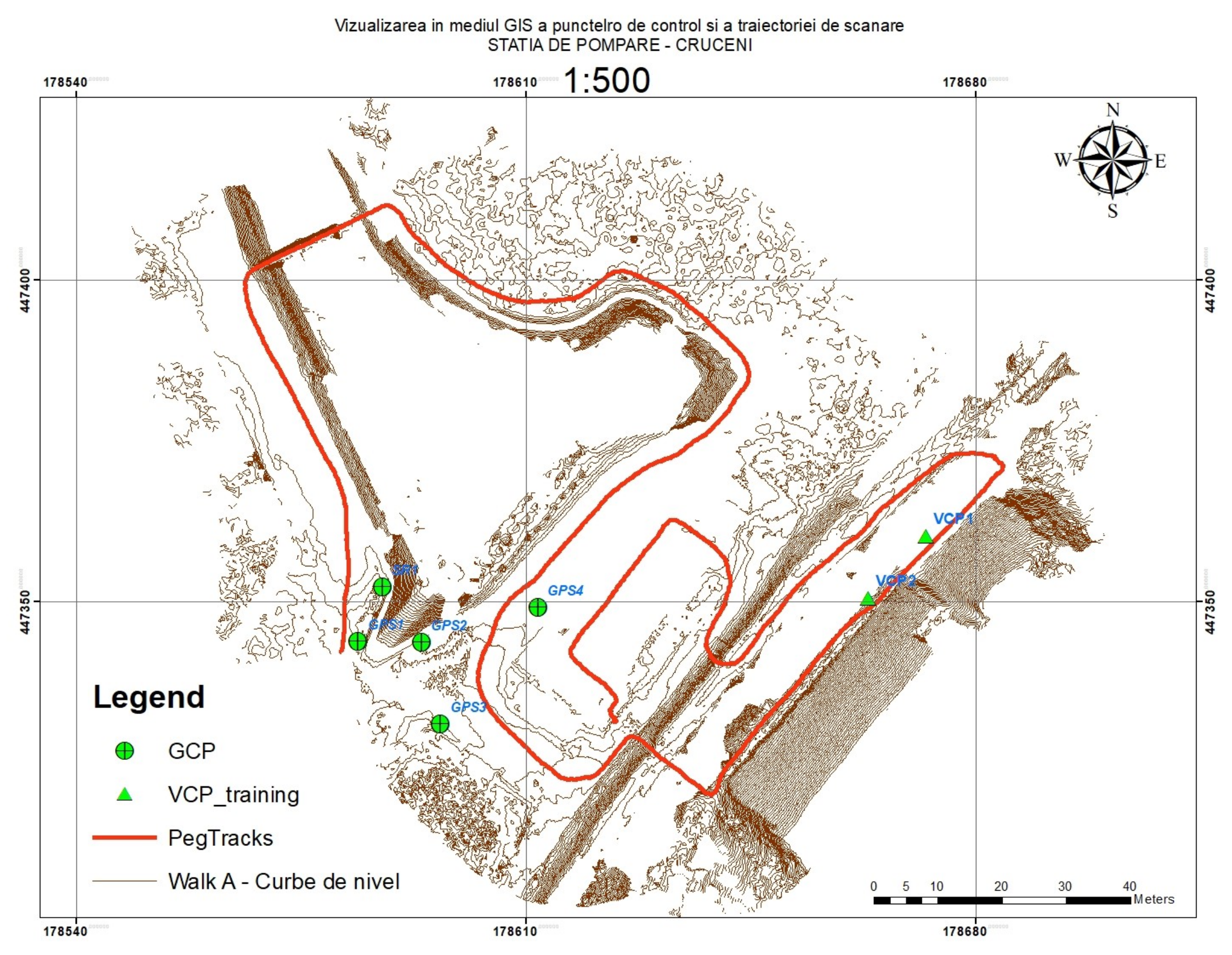
2.2.4. Cruceni Pumping Station

The civilian flood defence system has the major purpose of protecting urban and rural settlements, avoiding loss of life, and reducing material damage. Floods are the natural phenomenon that has marked and deeply marks the development of human society [46,47].

Statistics show us that in the period 2000–2009, floods had the highest frequency of all types of natural disasters. Out of an average of 387 natural disasters occurring during that aforementioned period, 173 (45%) were floods. In 2010, out of a total of 373 natural disasters, 182 (49%) floods were recorded. All this data is an additional argument in favour of preparations to deal with such events. Among the factors that favor the occurrence of floods we may mention climate change, soil compaction, and land consolidation that go hand in hand with intensive agriculture.

The floods in June-July 2010 affected 481 localities in 37 counties, with 20,000 people being recorded who were evacuated from their homes and about 4000 damaged households, of which 863 were completely destroyed. The damage caused by the floods in the summer of 2010 amounts to EUR 875 million according to assessments by the authorities. On 15 April 2005, Timiș County experienced the worst floods in the modern history of Banat. Following the rains and the melting of the ice, the Timis River exited the major riverbed causing damage of 150 million euros, according to estimates made by the authorities. The waters of the Timiș, Caraș and Bârzava rivers overflowed, resulting in the evacuation of 2800 people, the destruction of 5300 households, the damage of 4900 houses, of which 654 were completely destroyed, and the damage of 128,000 ha of land, 617 bridges, 300 km of roads (27.3 km of national roads, 92 km of county roads, 107 km of communal roads).

3. Results and Discussions

The purpose of this paper is conservation of the hydrotechnical heritage objectives using a different type of measurement tool through terrestrial 3D laser scans (the hydrotechnical nodes from Topolovăţu Mic [48] and Coșteiu, the lock from Sânmartinu Maghiar as well as the Cruceni pumping station) with the latest technologies.

The combined use of this equipment has been studied.

3.1. The Use of GNSS Technology to Thicken the Geodetic Network through Satellite Measurements for GCP Checkpoints

To be able to perform the measurements using the terrestrial laser scanner (TLS) and to be able to determine the coordinates of the ground control points GCP (Ground Control Point) used for checking and processing the SLAM for the mobile MMS laser scanning, a geodetic network was performed, using GNSS technology, static method [48,49].

The comparison of the data was done between the GNSS RTK values and the static GNSS values obtained from post-processing. The transcalculation of coordinates from the ETRS’89 reference system to the 1970 Stereographic system was performed with the TransDat 4.01 software produced by A.N.C.P.I. (Agency for Cadastre and Real Estate Advertising). The permanent GNSS stations from which the Rinex data was operated at 5s were Timisoara, Moldova Noua, and Arad (Romania) (

Table 4. GNSS permanent stations used in post-processing. Ellipsoidal coordinates—ETRS89.

Name of Standing Station	Class	B [m]	L [m]	He [m]
Arad (ARAD)	A	46°10′23.51004″ N	21°20′ 40.51052″ E	167.6742 m
Moldova Noua	A	45°51′16.42753″ N	22°10′ 37.78289″ E	216.4898 m
Timişoara 1 (TIM1)	A	45°46′47.65271″ N	21°13′ 51.46281″ E	154.7278 m

). By performing static measurements, the coordinates of the points of the thickening and lifting networks were obtained by determinations relative to the National Geodetic Network GNSS (RGN—GNSS) consisting of permanent GNSS stations (Class A) and stocking terminals (Class B, respectively Class C). It was mandatory to take into account the existence of visibility between the points of the lifting network.

3.1.1. Acquisition and Processing of Rinex Data

a. Preparatory phase

Preparatory stage—at this stage it is aimed at obtaining as much data as possible, comparing them to start the field stages. Thus, we recall the collection of data and the establishment of the working method and the necessary equipment.

Planning GPS measurements—in Figure 9a is presented GDOP for Topolovăţu Mic and in Figure 9b is presented the constellation and trajectory of satellites for Topolovăţu Mic.

Elevation of satellites

Another important element that was taken into account during the measurements was the elevation of the satellites. Even if for measurements it can be programmed that the receiver also records data from satellites below 15 degrees, it is necessary that when entering data in the program Leica Geo Office Combined to eliminate those that induce errors. Also, it was studied with the Almanac to see where it can be noticed if the PDO values met the conditions. We will present in Figure 10 the elevation of the satellites.

Stationary time on each concrete milestone.

In the case of static measurements made within the radius of Topolovăţu Mic Territory (Romania), the stationary time was 1.5 h for each measurement session (milestone). This means T = 60 min + 15 min = 75 min stationary time/milestone.

For an additional verification on the Feno type terminals that were located at the Topolovăţu Mic hydrotechnical node, determinations were also made in the kinematic mode (RTK-Real Time Kinematic) having a length of the session of about 600 s for each point. The WGS 1984 coordinates obtained from RTK readings were transformed directly into the field due to the implementation of the TransDatRO 4.06 [50] system directly in the controller.

b. Field stage

In the first phase, the recognition of the land was carried out, before planting the landmarks on the ground and in the second phase the actual measurements were made. Also in this phase, the field sheets were completed.

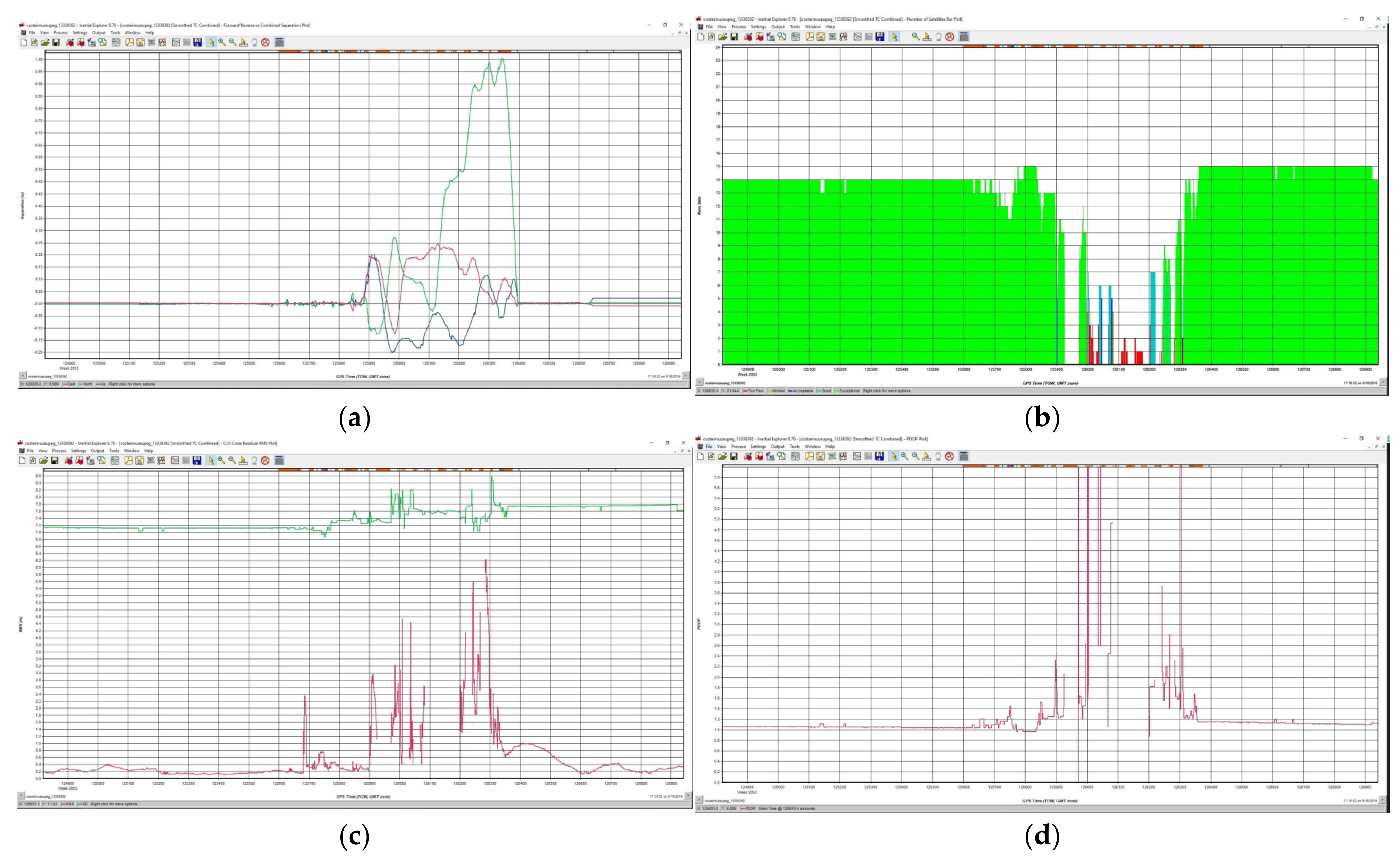
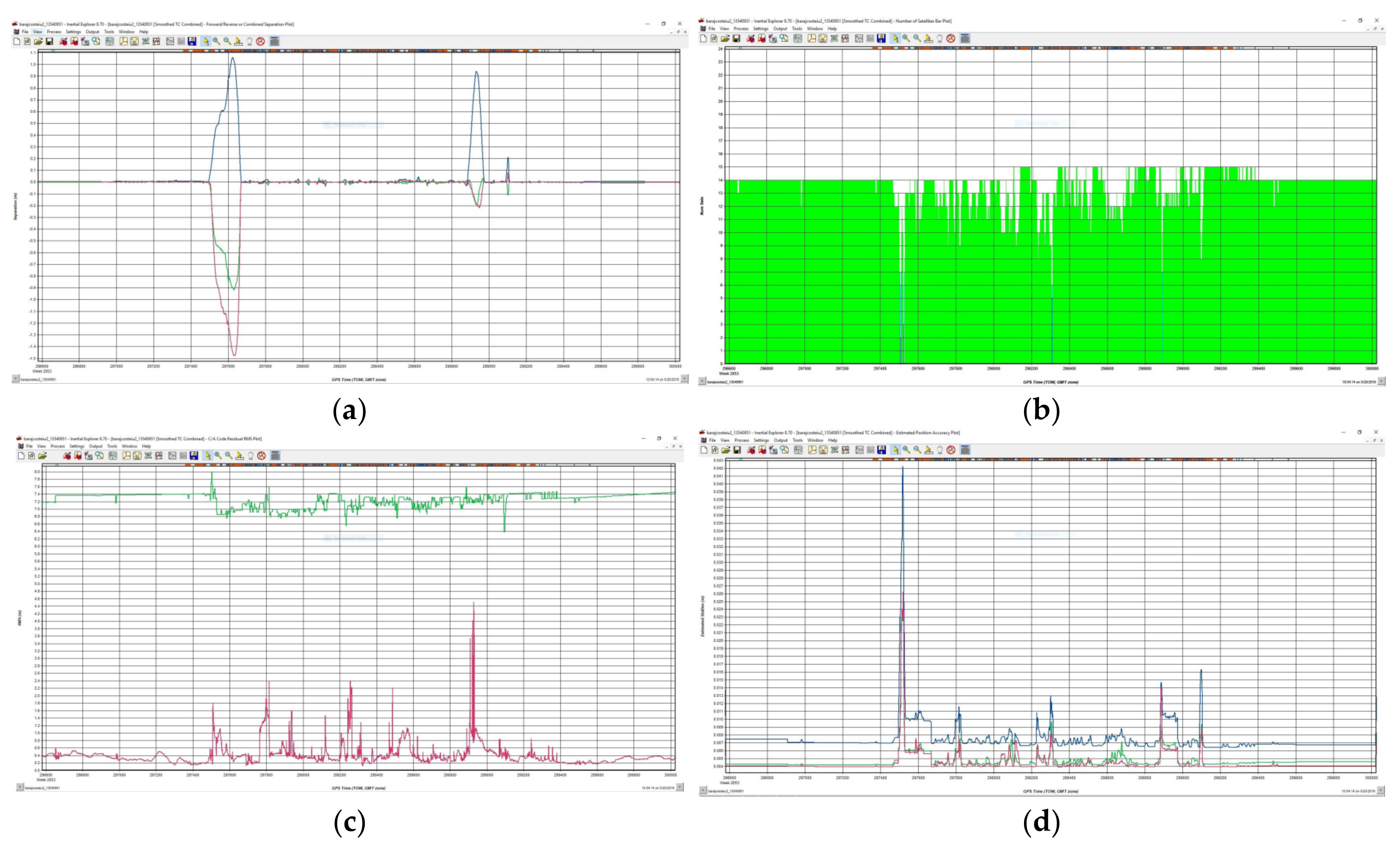
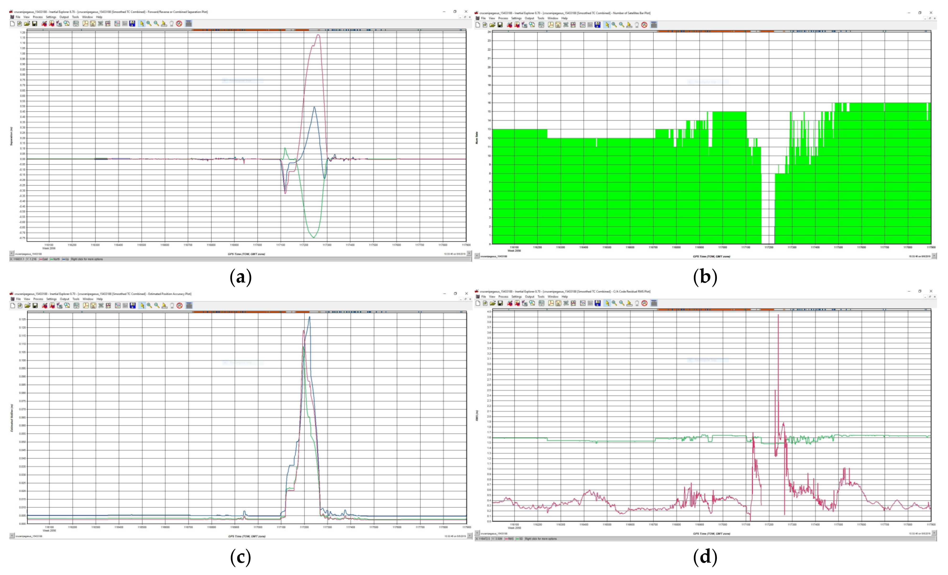
3.1.2. Postprocessing Data and Presentation of Obtained Results

At this stage, all the data files downloaded from the receivers into the software have been uploaded, the field sheets are carefully tracked. In the case of the paper, the filling in with the data referring to the height of the instrument has been carefully observed.

The software was used for data processing, a program that allows data processing and network clearing at the same time. The data files were imported in RINEX format-universally recognized format (Figure 11).

Table 5. Raw data entered in LGO, Topolovăţu Mic with corrected stations.

No.Pct	Point Class	Duration of Measurement	GNSS	Type of Measurement	Measuring Height
TIM1	Control	9h 59′55″	GPS/GLONASS	Static	0,0000
MOLD	Control	9h 59′55″	GPS/GLONASS	Static	0,0000
FAGE	Control	9h 59′55″	GPS/GLONASS	Static	0,0000
TMIC2	Measured	2h 18′20″	GPS/GLONASS	Static	2,0000
TMIC1	Measured	1h 52′49″	GPS/GLONASS	Static	2,0000
TMIC3	Measured	1h 55′55″	GPS/GLONASS	Static	2,0000
TMIC8	Measured	1h 23′30″	GPS/GLONASS	Static	2,0000
TMIC9	Measured	1h 23′15″	GPS/GLONASS	Static	2,0000

presents the data entered in the processing software. In

Table 6. Fulfillment or non-fulfilment of ambiguities, Topolovăţu Mic, Timiș County.

No.pct	Era 10/13/2017/hour	Status of Ambiguities	Type of Measurement	Solution	East	North
TMIC2	11:07:32	not	Static	Float	45°45′43.93254″ N	21°38′08.85145″ E
TMIC2	11:07:32	yes	Static	fixed all	45°45′43.93126″ N	21°38′08.84424″ E
TMIC2	11:07:32	yes	Static	fixed all	45°45′43.93198″ N	21°38′08.84525″ E
TMIC1	13:32:07	not	Static	Float	45°45′42.05516″ N	21°38′08.62780″ E
TMIC1	13:32:07	yes	Static	fixed all	45°45′42.05499″ N	21°38′08.62696″ E
TMIC1	13:32:07	yes	Static	fixed all	45°45′42.05534″ N	21°38′08.62661″ E
TMIC3	13:37:27	not	Static	Float	45°45′42.22913″ N	21°38′12.53778″ E
TMIC3	13:37:27	yes	Static	fixed all	45°45′42.22745″ N	21°38′12.53795″ E
TMIC3	13:37:27	yes	Static	fixed all	45°45′42.22853″ N	21°38′12.53784″ E
TMIC8	13:44:42	not	Static	Float	45°45′36.81844″ N	21°38′08.30090″ E
TMIC8	13:44:42	yes	Static	fixed all	45°45′36.81829″ N	21°38′08.29966″ E
TMIC8	13:44:42	yes	Static	fixed all	45°45′36.81865″ N	21°38′08.29931″ E
TMIC9	13:48:17	not	Static	Float	45°45′35.75665″ N	21°38′09.21471″ E
TMIC9	13:48:17	yes	Static	fixed all	45°45′35.75523″ N	21°38′09.21749″ E
TMIC9	13:48:17	yes	Static	fixed all	45°45′35.75627″ N	21°38′09.21732″ E

and

Table 7. Post-processing static network by satellite measurements, Topolovăţu Mic.

Item No.	Height on Ellipsoid	Orthometric Height	Geoid	Error on X (m)	Error on Y (m)	Error 3D (m)
TMIC2	361.919	1.024.098	−662.179	0.0064	0.0026	0.0069
TMIC2	361.645	1.023.824	−662.179	0.0004	0.0007	0.0008
TMIC2	363.487	1.025.665	−662.179	0.0004	0.0006	0.0007
TMIC1	357.380	1.019.559	−662.179	0.0013	0.0009	0.0016
TMIC1	355.909	1.018.089	−662.179	0.0005	0.0008	0.0010
TMIC1	357.909	1.020.088	−662.179	0.0003	0.0005	0.0006
TMIC3	388.222	1.050.411	−662.190	0.0045	0.0038	0.0059
TMIC3	385.761	1.047.950	−662.190	0.0004	0.0007	0.0008
TMIC3	387.686	1.049.876	−662.190	0.0004	0.0006	0.0007
TMIC8	363.351	1.025.532	−662.181	0.0021	0.0014	0.0026
TMIC8	362.025	1.024.206	−662.181	0.0005	0.0007	0.0009
TMIC8	363.957	1.026.138	−662.181	0.0004	0.0006	0.0007
TMIC9	364.074	1.026.258	−662.184	0.0056	0.0040	0.0069
TMIC9	361.688	1.023.872	−662.184	0.0005	0.0007	0.0009
TMIC9	363.626	1.025.810	−662.184	0.0005	0.0007	0.0008

, we can see the fulfillment or non-fulfilment of ambiguities as well as the accuracies obtained.

After processing the data, we proceeded to adjust the network with the Leica Geo Office Combined program and to compare the data obtained, those by Static methods with those obtained by RTK method (

Table 8. Coordinate inventory of new points in WGS 84 system, Topolovăţu Mic.

Coordinates WGS 1984
Station Name	Coordinates		Corrections	Sd
TMIC1	Longitude	21°13′51.46271″ E	0.0000 m	-
	Height	154.7278 m	0.0000 m	-
TMIC2	Latitude	45°45′44.01926″ N	−0.0004 m	0.0271 m
	Longitude	21°38′08.84475″ E	0.0032 m	0.0212 m
	Height	145.6545 m	0.0000 m	0.0612 m
TMIC3	Latitude	45°45′42.31566″ N	−0.0004 m	0.0293 m
	Longitude	21°38′12.53784″ E	0.0032 m	0.0220 m
	Height	148.0696 m	0.0000 m	0.0547 m
TMIC8	Latitude	45°45′36.90617″ N	−0.0004 m	0.0320 m
	Longitude	21°38′08.29941″ E	0.0032 m	0.0224 m
	Height	145.7076 m	0.0000 m	0.0568 m
TMIC9	Latitude	45°45′35.84338″ N	−0.0004 m	0.0344 m
	Longitude	21°38′09.21734″ E	0.0032 m	0.0251 m
	Height	145.6592 m	0.0000 m	0.0611 m

,

Table 9. Coordinate inventory of new points in Stereographic System 1970, resulting from transformations for STATIC measurements, Topolovăţu Mic.

1970 Stereographic Coordinates
Station	Coordinates		Corrections	Sd
FAGE	Y(m)	280,960.4506 m	0.0000 m	-
	X (m)	487,749.6411 m	0.0000 m	-
	Z (m)	173,080 m	0.0000 m	-
TIM1	Y(m)	207,132.2474 m	0.0000 m	-
	X (m)	482,495.1249 m	0.0000 m	-
	Z (m)	111.641 m	0.0000 m	-
TMIC1	Y(m)	238,501.5611 m	0.0032 m	0.0208 m
	X (m)	479,067.2393 m	−0.0006 m	0.0280 m
	Z (m)	101.950 m	0.0000 m	0.0536 m
TMIC2	Y(m)	238,508.7103 m	0.0032 m	0.0212 m
	X (m)	479,124.9330 m	−0.0006 m	0.0271 m
	Z (m)	102.483 m	0.0000 m	0.0612 m
TMIC3	Y(m)	238,586.2440 m	0.0032 m	0.0220 m
	X (m)	479,069.0104 m	−0.0006 m	0.0293 m
	Z (m)	104.900 m	0.0000 m	0.0547 m
TMIC8	Y(m)	238,487.6787 m	0.0032 m	0.0224 m
	X (m)	478,905.9765 m	−0.0006 m	0.0320 m
	Z (m)	102.539 m	0.0000 m	0.0568 m
TMIC9	Y(m)	238,506.1187 m	0.0032 m	0.0251 m
	X (m)	478,872.3513 m	−0.0006 m	0.0344 m
	Z (m)	102.491 m	0.0000 m	0.0611 m

,

Table 10. 1970 Stereographic coordinates obtained by CINEMATIC measurements (RTK).

Point No.	Stereographic Coordinates 1970 Static Reading (RTK)
	X (m)	Y (m)	Z (m)
TMIC1	479,067.286	238,501.567	102,111
TMIC2	479,124.943	238,508.712	102,647
TMIC3	479,069.033	238,586.241	105,086
TMIC8	478,905.988	238,487.673	102,689
TMIC9	478,872.351	238,506.115	102,642

,

Table 11. 1970 Stereographic coordinates obtained by STATIC measurements after post-processing.

Point No.	Stereographic Coordinates 1970 Results from Post-Processing (STATIC)
	X (m)	Y (m)	Z (m)
TMIC1	479,067.239	238,501.561	101,950
TMIC2	479,124.933	238,508.710	102,483
TMIC3	479,069.010	238,586.244	104,900
TMIC8	478,905.976	238,487.679	102,539
TMIC9	478,872.351	238,506.119	102,491

,

Table 12. Coordinate differences between KINEMATIC (RTK) and STATIC measurements, resulting from field measurements and post-processing.

Point No.	Coordinate Differences RTK vs. STEREO
	X (m)	Y (m)	Z (m)
TMIC1	0.047	0.006	0.161
TMIC2	0.010	0.002	0.164
TMIC3	0.023	−0.003	0.186
TMIC8	0.012	−0.006	0.150
TMIC9	0.000	−0.004	0.151

and

Table 13. Coordinate differences between KINEMATIC (RTK) and STATIC measurements, resulting from field measurements and post-processing in AutoCAD.

Point No.	RTK vs. STEREO Coordinate Differences
	(m)	(cm)
TMIC1	0.010	1
TMIC2	0.050	5
TMIC3	0.020	2
TMIC8	0.010	1
TMIC9	0.000	0

).

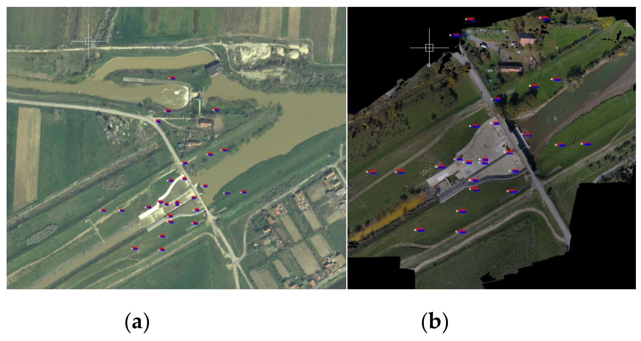
3.2. Data Acquisition and Processing Using UAV Technology in the Studied Facilities

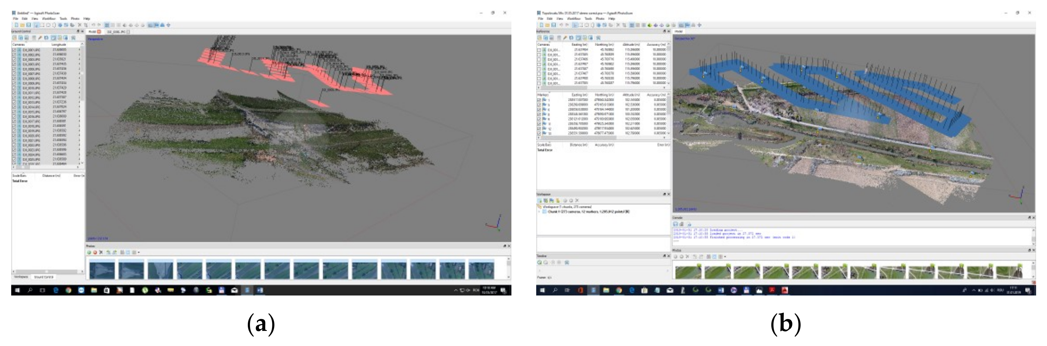
3.2.1. Photogrammetric Data Processing

In terms of photogrammetric data analysis, software programs use different approaches, both with commercial and open-source solutions [51].

In order to carry out the research and to be able to make a comparison of the data, several flight sessions have been carried out for the heritage objectives researched within the present work, where only 2 flight sessions will be presented (due to the large volume of data), made for the Topolovăţu Mic Hydrotechnical Node. Import of photos: it is the first step that will be done in order to carry out the processing of photogrammetric data. Regarding the two sessions, 50 aerial images were collected in the first session and in the second one, 287 images. Aligning images with PhotoScan Professional: the algorithm looks for common points on the images and matches them by finding the camera position for each image, estimating the camera calibration parameters. The program then calculates the positions of the camera and generates the first point cloud (Figure 12a,b).

3.2.2. Developing the Digital Elevation Model

PhotoScan [52] allows to perform measurements of point, distance, area, volume based on DEM, as well as the generation of cross-sections for a part of the selected scene by the user. In addition, contour lines can be calculated for the 3D model and are represented either over DEM images or over Orthomosaic.

To generate the digital elevation model (DEM), it is necessary to first classify dense cloud points to divide them into at least two classes: ground points and the rest. For this, the base value for the class parameter should first be selected in the Build DEM dialogue to generate the DEM.

The resolution value shows an actual ground resolution for the DEM, estimated for the source data. The resulting DEM size, calculated in relation to the ground resolution, is shown in the total size text box.

Session I-a was made up of 80 million points (80,371,748 points) obtained with high resolution (Ultra high quality), and the 3D model consisted of 16 million faces (16,054,425 faces). The whole processing took about 12 h. The resolution of the DEM was 3.46 cm/pix. (14,875 × 144,414).

Session II consisted of 32 million points (32,119,012 points) obtained with high resolution (High quality), and the 3D model consisted of 6 million faces (6,458,745 faces). The whole processing took about 5 h. The DEM resolution in this case was 8.28 cm/pix. (8196 × 5180).

One may notice that although the first session had only 50 images of which 48 images remained for photogrammetric processing, the processing time was more than double, resulting in an accuracy of 3.46 cm/pixel, while session II had 5 times more images, namely 287, of which 273 images remained for processing; the quality of the orthophotoplane obtained is much lower, which can be seen from the resolution per pixel which is 8.28 cm, almost 3 times lower (Figure 13).

Triangular photogrammetry can be used to generate an orthophoto image and a DSM. These products were generated, in our case with a resolution of 0.05 m.

The dense clouds of 3D points for NH Coșteiu, based on UAV images, consisted of 43 million points (42,517,472 points) obtained with high resolution (Ultra high quality), and the 3D model consisted of 2 million faces (2,834,498 faces). The whole processing took about 8 h. The resolution of the DEM was 6.99 cm/pix (9778 × 8718).

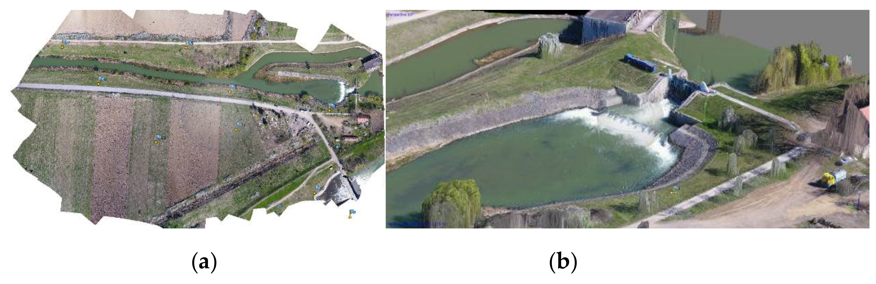
3.2.3. Orthomosaic and Orthophotoplane Production

Orthomosaic export is normally used to generate high-resolution images based on aerial photographs and the reconstituted model. The most common application is the processing of aerial photographic data, but it can also be useful when a detailed view of the object is required. PhotoScan [53] allows performing orthotomosaic editing in a straight line for better visual results.

PhotoScan [53] generates orthomosaics for the entire area, where surface data is available. The limitations of the limitation boxes were not applied. To build an orthophotoplan, for a specific (rectangular) part of the research, the Region section of the Build Orthomosaic dialogue (Figure 14a,b) was used.

A comparative analysis of the resulting georeferencing data was also made by comparing two orthophotoplans: one from 2015, made by the ANCPI and the the second one conducted in the research in 2018. Figure 15a,b shows the georeference orthophotoplan for HN Topolovăţu Mic.

3.3. GIS Data Acquisition and Processing Using TLS Technology

The digital preservation of cultural heritage monuments is a 3D modeling challenge. Objects and cultural heritage sites differ greatly from one to the other [54], and a fidelity of 3D modeling is an essential condition. Terrestrial laser scanning is a 3D technology that, lately, has become increasingly known, especially for the possibility that it offers the benefit of making a documentation that offers very dense 3D points on a surface with high accuracy. Therefore, the resulting 3D models can be used to produce a digital documentation, as well as the possibility of performing analysis, such as: measurements, monitoring, preservations, detail extractions, and virtual restoration [55].

UAV-LiDAR will therefore allow to ask new questions on large-scale hydrological connectivity in complex landscapes with an important relevance to the WRM.

Each scan was performed on the topographical principle of orientation of the device using the method of known coordinates, coordinates marked in the field by FENO type terminals, whose coordinates were determined by satellite measurements using the STATIC method of determining the position and recording of RINNEX data at an interval of 5 s [56].

The final 3D model was obtained by integrating point clouds (Point Cloud) from aerial scans (UVS) with point clouds resulting from terrestrial ones (TLS), but only after the UAV point clouds were georeferenced and defined in a single frame of unique reference: Stereographic 1970 and Black Sea 1975, respectively.

3.3.1. TLS Data Acquisition

The results obtained by merging the point clouds required the use of a PC computer (high-performance graphics station, due to the large volume of data) Intel Core i7, Windows 10, 16 GB of RAM, resulting in a processing time of about 2–3 h, with the final result being a 3D points cloud.

The location for performing scans and obtaining point clouds is located in five places in Timiș County (NH Coşteiu, NH Topolovăţu Mic, NH Sânmihaiu Român, NH Sânmartinu Maghiar and Cruceni pumping station) where, for the measurements, a high-precision 3D laser scanner from Leica was used, the ScanStation Leica C10 model, which records the geometry of the surfaces and structures, thus rendering the digital image of the scanned lens and the laser data was processed using version 9.3.1. of the Cyclone program.

To complete the digital model for the upper part of the heritage objectives we have used the UAV technique, namely a Phantom4 Pro drone, which was correlated with the TLS (Terrestrial Laser Scanner) technique through specialised programs.

The current scientific paper consists of producing and processing the sets of measurements made in the field with the ScanStation Laica C10 scanner for the locations under study.

Performing measurements using the Leica ScanStation C10 scanner can be presented in four stages, namely: planning measurements, scanning itself, downloading data from the device, and processing the data.

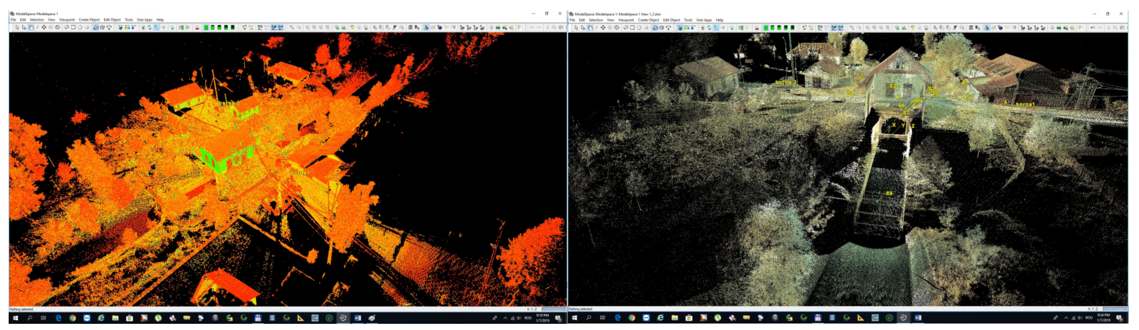
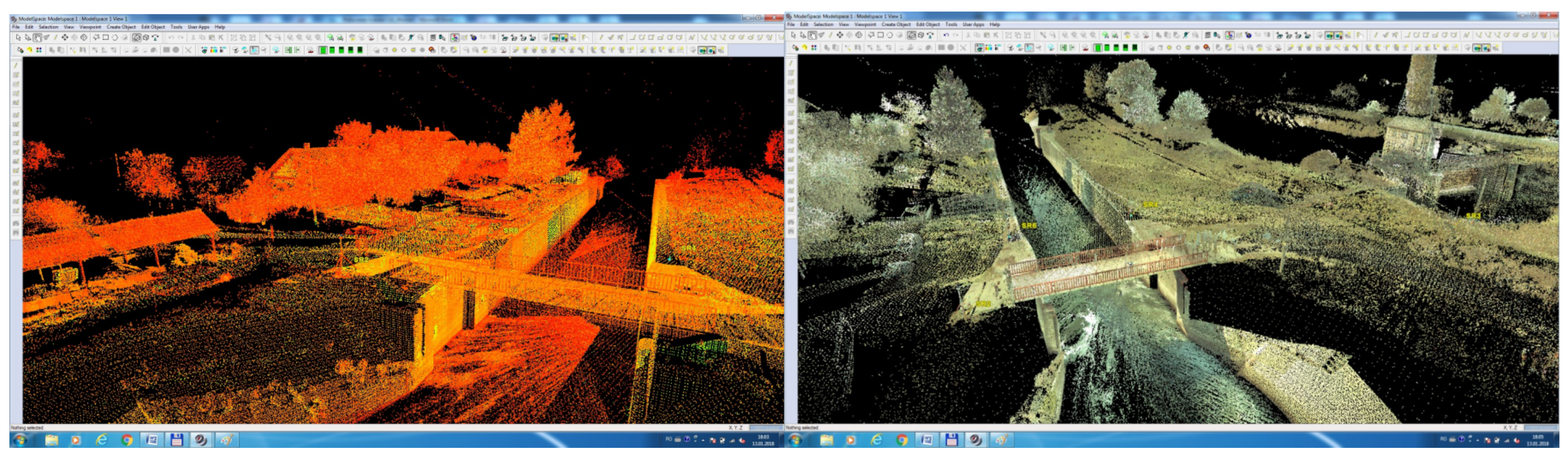
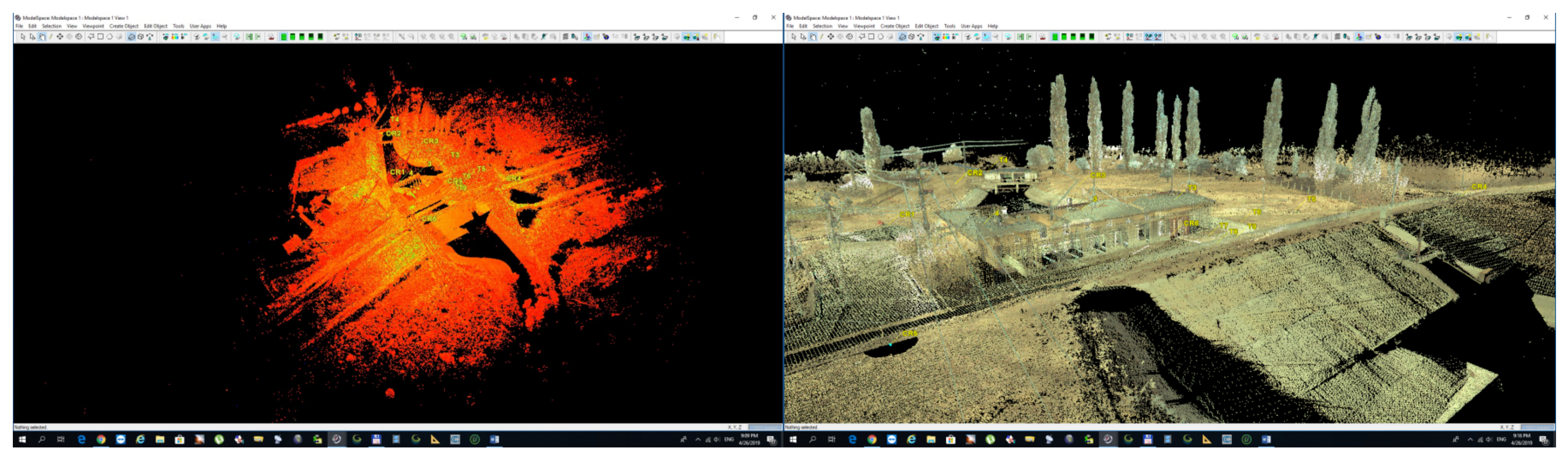
3.3.2. Data Processing and Obtaining 3D Point Clouds

The processing of measurements was carried out with the program Cyclone 9.3 version 9.3.1. A first step is to import the raw data into the Cyclone program. After the introduction of the scans, the Cyclone program includes relative alignment of the setups to each other, which can be done manually or automatically. The alignment of the scans made, from different stations to a single common station, can be done either with the option ‘Smart Align’ (direct station alignment technique) or by a ‘Manual Registering’ (indirect station alignment technique) called georeference, and at the end we can also perform a pre-visualization of the scans, the recorded constraints and errors.

The recording of the resulting point clouds, coming from different stations, consists of entering the scans named ‘ScanWorld’ in one single ‘Registration’ record, adding some automatic constraints of cloud points type, “Control Spaces”.

The position of each scanning station is defined by the coordinates entered in the scanner. In order to be able to achieve the alignment of the scanning positions it is necessary to know the position and the orientation, according to a coordinate system (

Table 14. Position and orientation of the Leica C10 scanner, NH Coșteiu, ID costei1.

Project	Station Point	ScanWorld	Date	Time	Method
Scan Costei1	Costa 1-GPS	sw-003	20.10.2017	12.09.53	“Known Backsight”
Position: 0.006 m; Height: 0.004 m
Observation
Name	East Y (m)	North X (m)	Share Z (m)	Target H (m)	Target type
Costei1	255,279.914	475,633.333	116.820	2.170	HDS Tgt 6 inches
Residual value
Name	δx	δy	δz	ΔHz
Costei2	−0.003	−0.004	0.011	0.005
Result
Name	Est Y (m)	North X (m)	Share Z (m)	Scanner H (m)	Orientation [°]
Costei1	255,245.829	475,594.854	116.716	1.621	−33.1794
Accuracy	Position	0.006	Altitude	0.004

,

Table 15. Position and orientation of the Leica C10 scanner, NH Coștei, ID costei3.

Project	Station Point	ScanWorld	Date	Time	Method
Scan Costei1	Costa 1-GPS	sw-003	20.10.2017	12.09.53	“Known Backsight”
Position: 0.006 m; Height: 0.004 m
Observation
Name	East Y (m)	North X (m)	Share Z (m)	Target H (m)	Target type
Costei1	255,245.817	475,594.846	116.702	2.170	HDS Tgt 6 inches
Residual value
Name	δx	δy	δz	ΔHz
Costei2	−0.012	−0.012	−0.014	0.014
Result
Name	Est Y (m)	North X (m)	Share Z (m)	Scanner H (m)	Orientation [°]
Costei1	255,206.308	255,206.308	114.305	1.515	−34.2774
Accuracy	Position	0.006	Altitude	0.004

and

Table 16. Position and orientation of the Scanner Leica C10, NH Coștei, ID costei4.

Project	Station Point	ScanWorld	Date	Time	Method
Scan Costei1	Costa 1-GPS	sw-003	20.10.2017	12.09.53	“Known Backsight”
Position: 0.006 m; Height: 0.004 m
Observation
Name	East Y (m)	North X (m)	Share Z (m)	Target H (m)	Target type
Costei3	255,206.308	475,565.924	114.261	2.170	HDS Tgt 6 inches
Residual value
Name	δx	δy	δz	ΔHz
Costei3	−0.000	−0.000	0.004	0.000
Result
Name	East Y (m)	North X (m)	Share Z (m)	Scanner H (m)	Orientation [°]
Costei4	255,184.348	475,493.796	110.542	1.586	−11.6676
Accuracy	Position	0.006	Altitude	0.004

). After viewing the recorded errors in each station, one can proceed further to the realization of the 3D model of the scanned lenses and the visualization of the 3D models (Figure 16, Figure 17, Figure 18 and Figure 19), with the possibility of cleaning the 3D model (such as 3D points recording from the station at the time of contact of the lens with the sun, passing people, cars, etc.).

With the help of this program, the alignment of the clouds of points obtained from the UAV flights for the completion of the upper parts were also achieved (for example, the roof), by identifying as many as possible common points in point clouds resulting from terrestrial scanning with the ScanStation Leica C10 scanner.

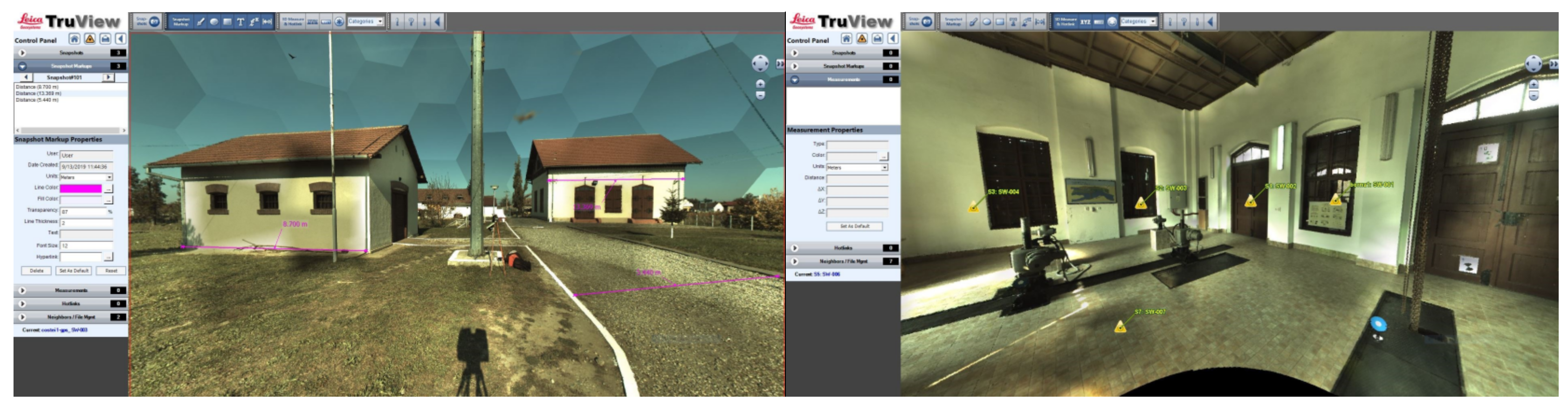
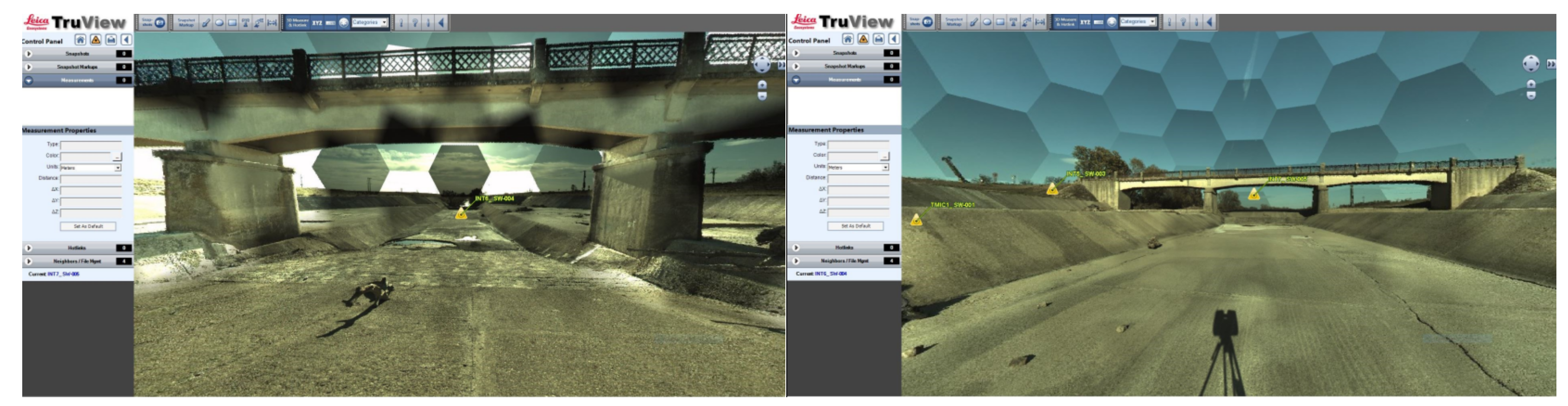
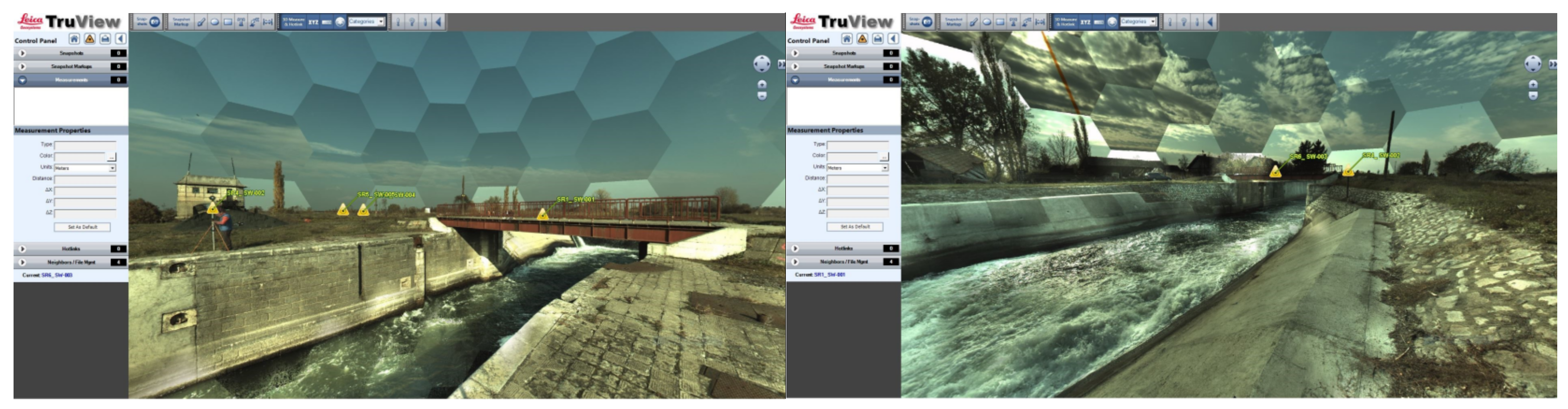
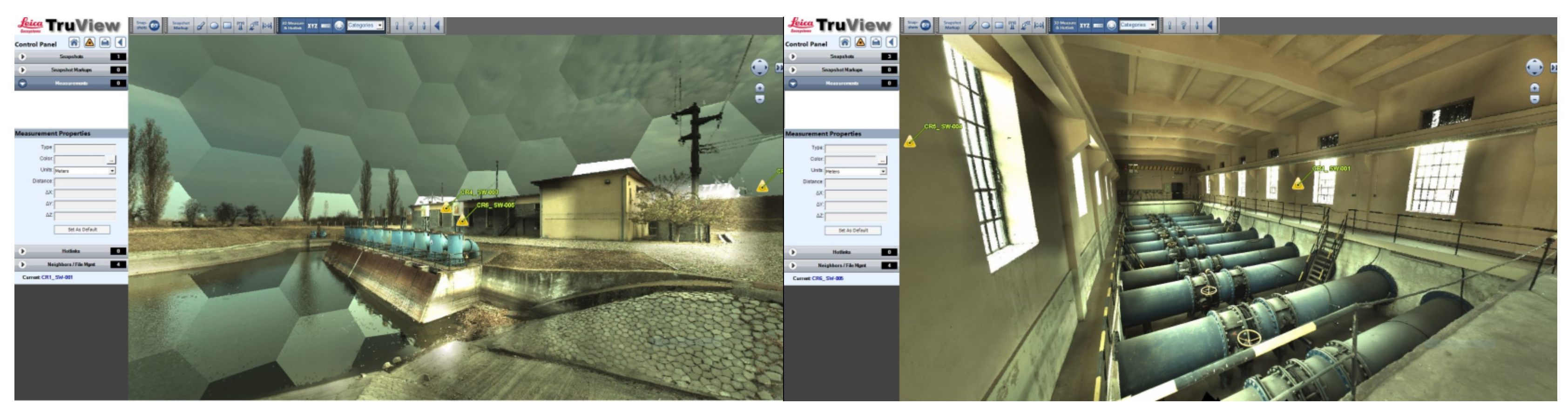
3.3.3. Making the Virtual Tour (TruView)

At the end of the work, the data were exported in different formats required by the architect: * .E57; * .ptx; * .x,y,z. For the presentation and visualization of historical monuments, a directory link was created, which can be directly accessed, and trough which, a virtual heritage tour can be made, TruViewSetup32-309.exe.

The TruView site map is a panoramic image (360 degree) of data from cloud points, the view being located in the same location as the scanner that captured the point clouds. The point of view in TruView is made exactly from the location where the scanner was placed and where the scanning of each lens took place. With the help of this program, you can achieve increases and decreases around the stage while extracting the dimensions from one point to another and extracting coordinates, but it will not be possible to fly around the stage as in some 3D systems.

After creating the TruView link, it was possible to move from one location of the scanner to another in order to have different points of view within the project. Each point of view has a separate ScanWorld. The site map contains image icons located in the center of each available TruView scene, where with a single click on an icon, which is triangle type, we will have another point of view from another station. TruView may be launched directly from Internet Explorer.

The data processing, obtaining the TruView link, as well as the data processing report and the errors recorded when performing the scans for the Coșteiu Hydrotechnical Node are shown in Figure 20; for the Topolovăţu Mic Hydrotechnical Node, they are shown in Figure 21; for the Sânmihaiu Român Lock, they are shown in Figure 22; for the Sanmartinu Maghiar Lock, they are shown in Figure 23; and for the Cruceni Pumping Station, they are shown in Figure 24.

3.4. GIS Data Acquisition and Processing Using Mobile LiDAR Technology (MMS)

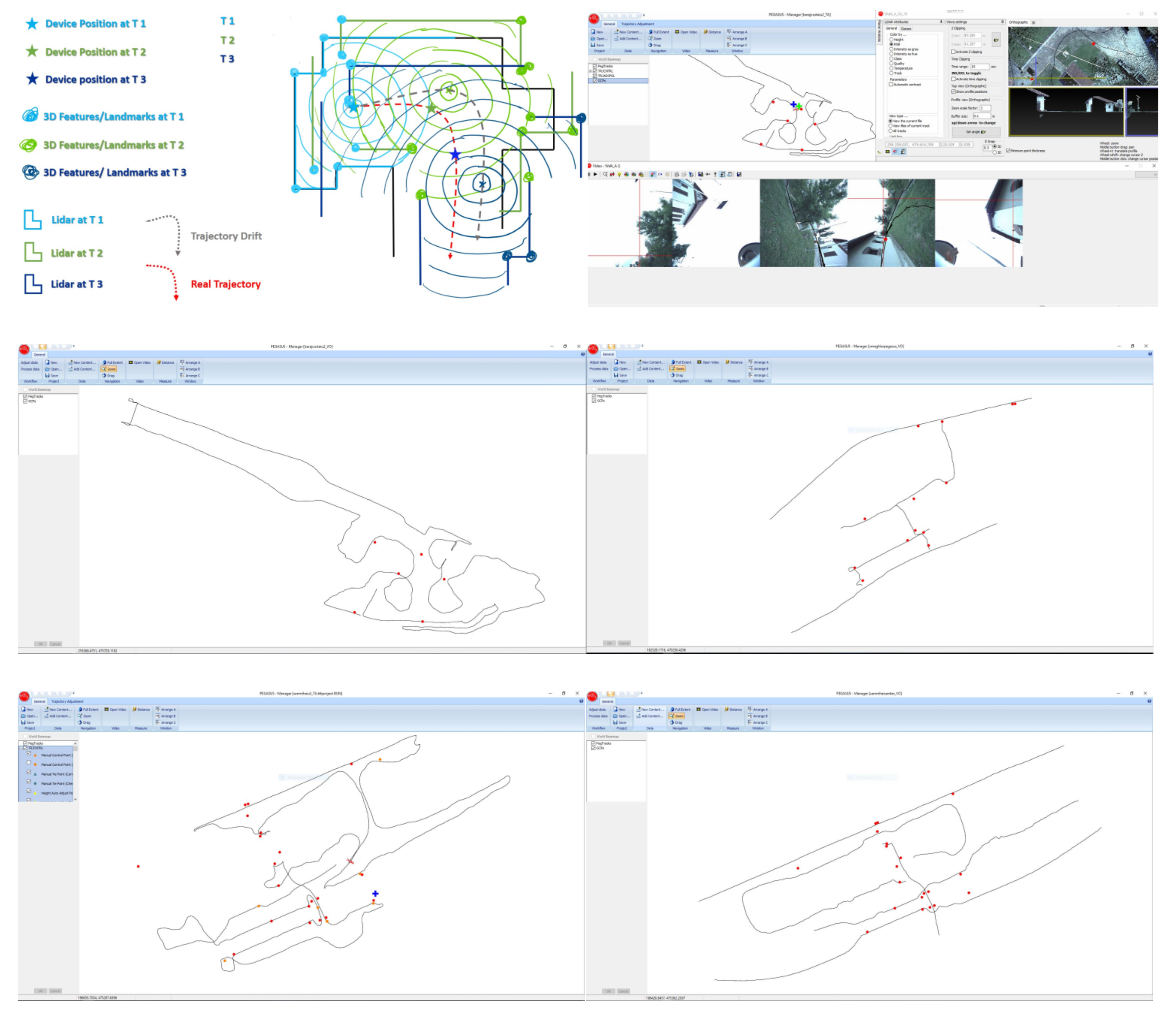
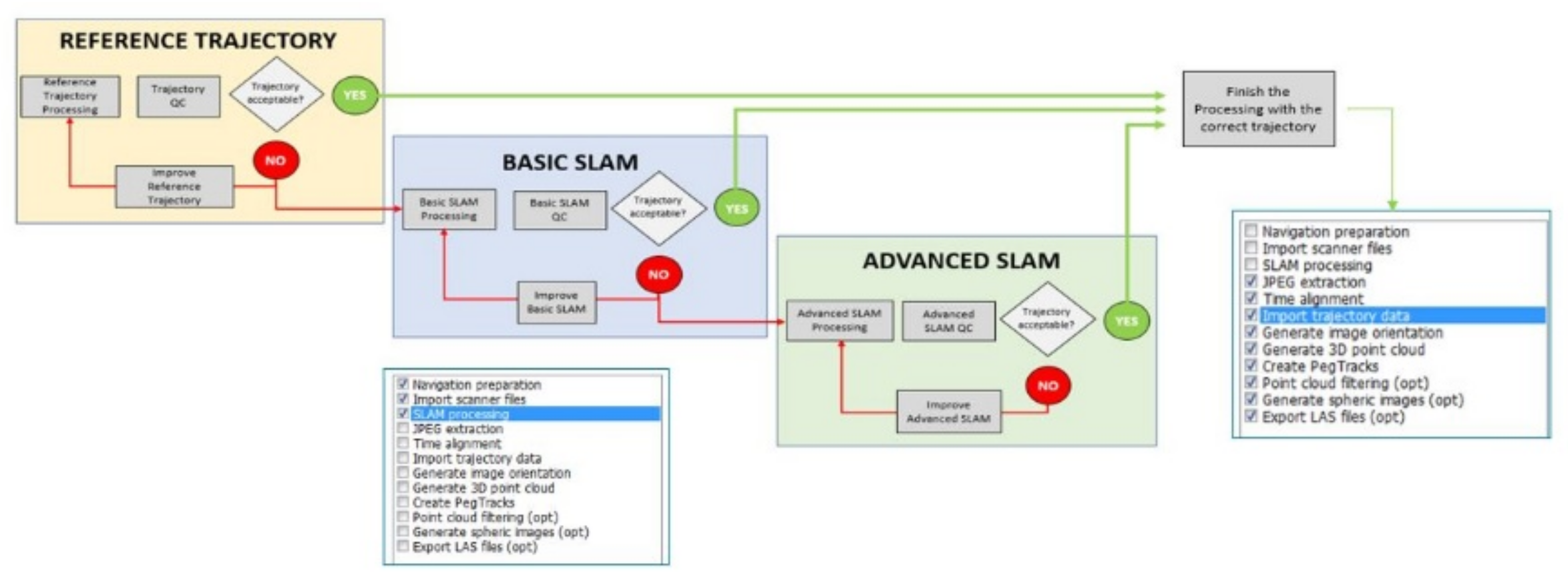
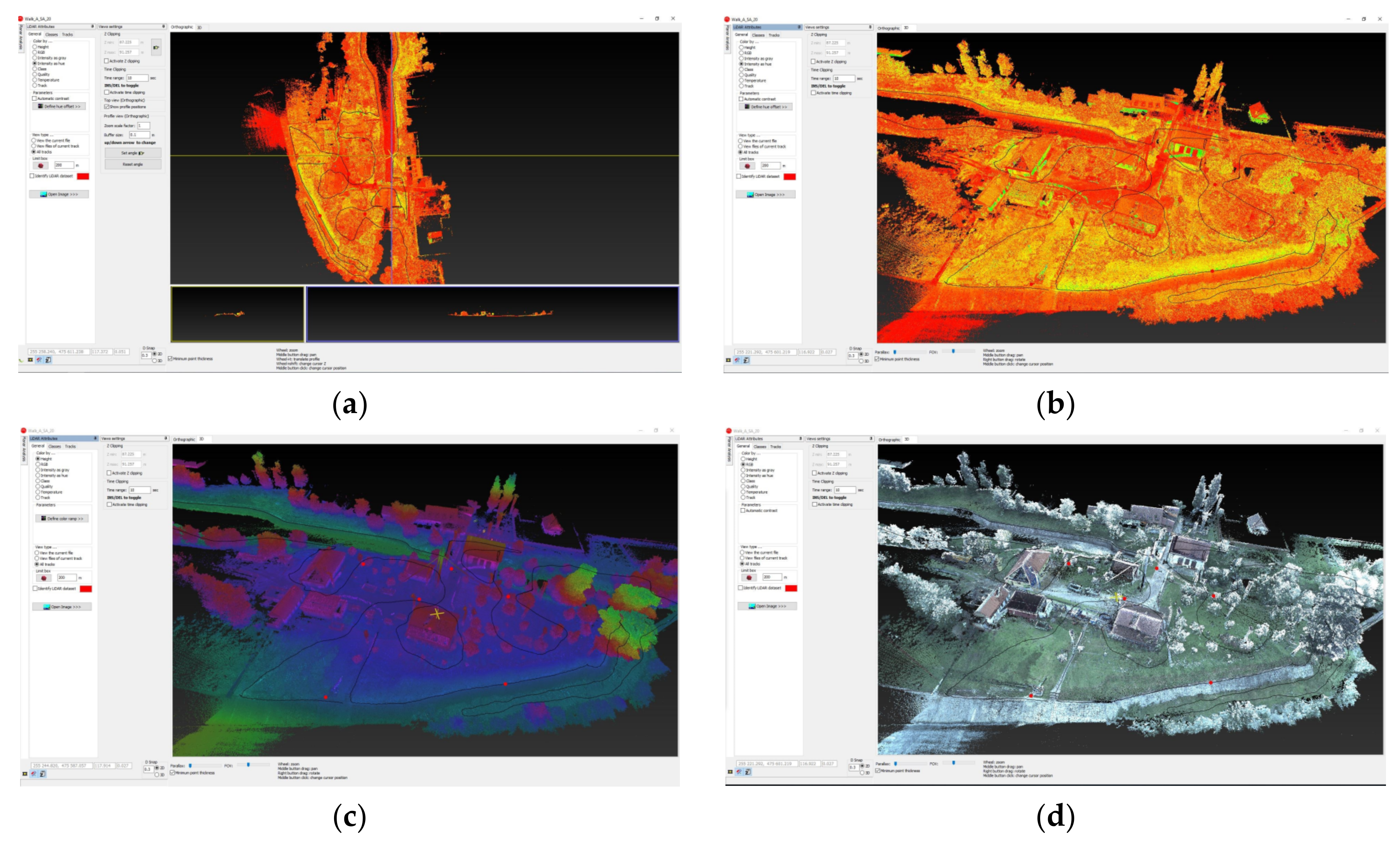
3.4.1. Pre-Processing of LiDAR Data and Data Visualization in QC Tools

Viewing the processing of the LiDAR scan trajectory, the correctness of the data collection and the visualization of the measurement quality (QC Tools) will be done in the Inertial Explorer program (Figure 25), using the graphs presented below (Figure 26, Figure 27, Figure 28 and Figure 29).

Within each group, the plots appear in alphabetical order in three colors: green, blue, and black. Green plots are generally the most frequently accessed plots, blue parcels less, and black parcels are rarely accessed, except for advanced users.

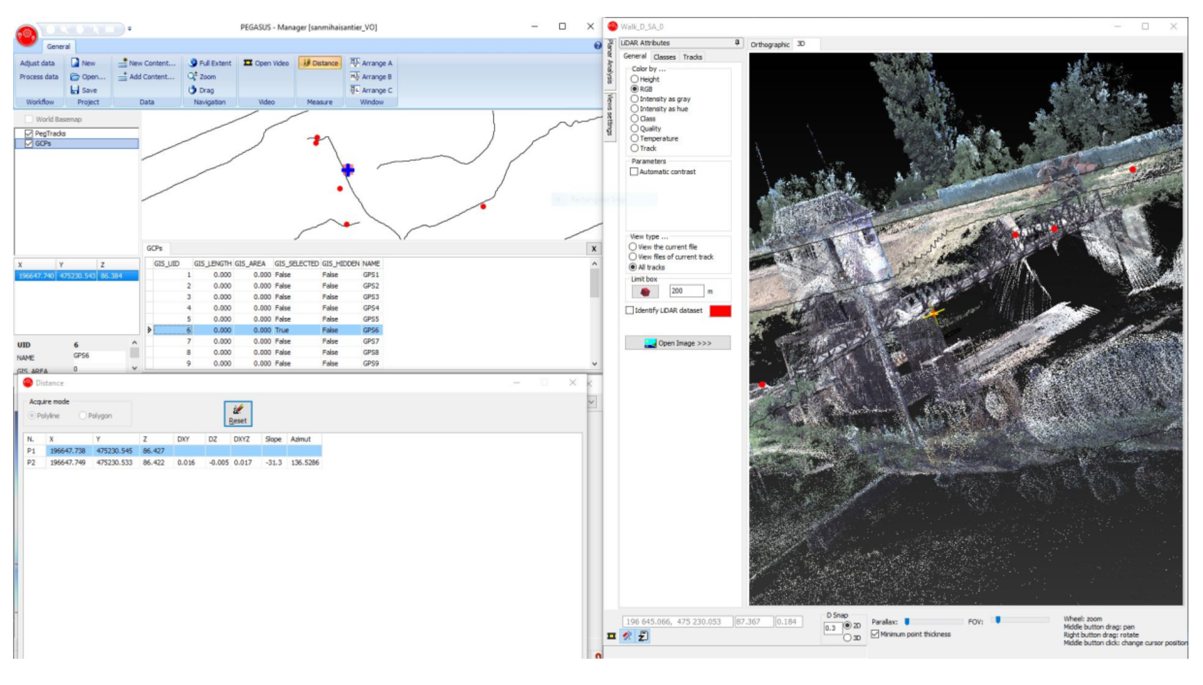
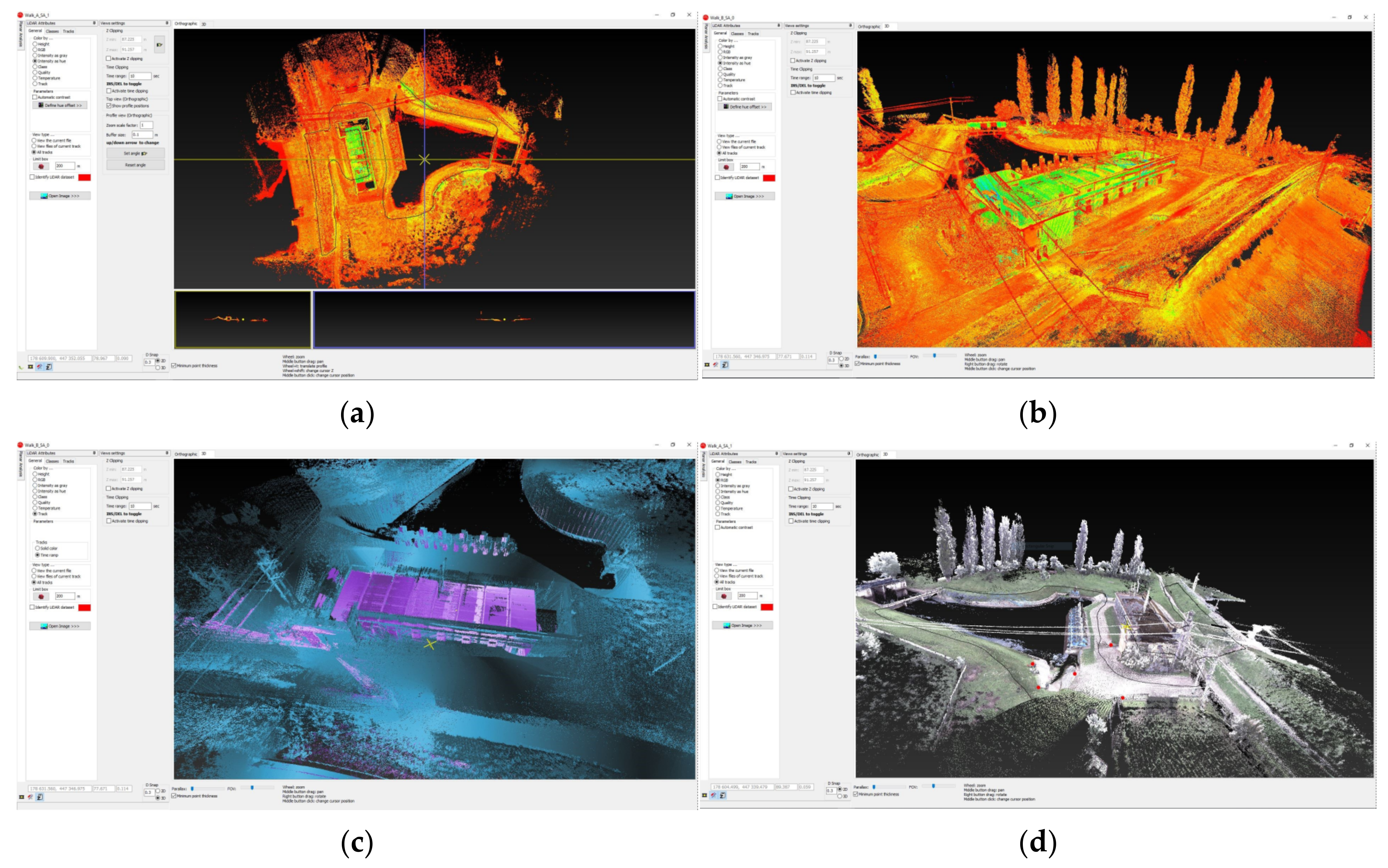
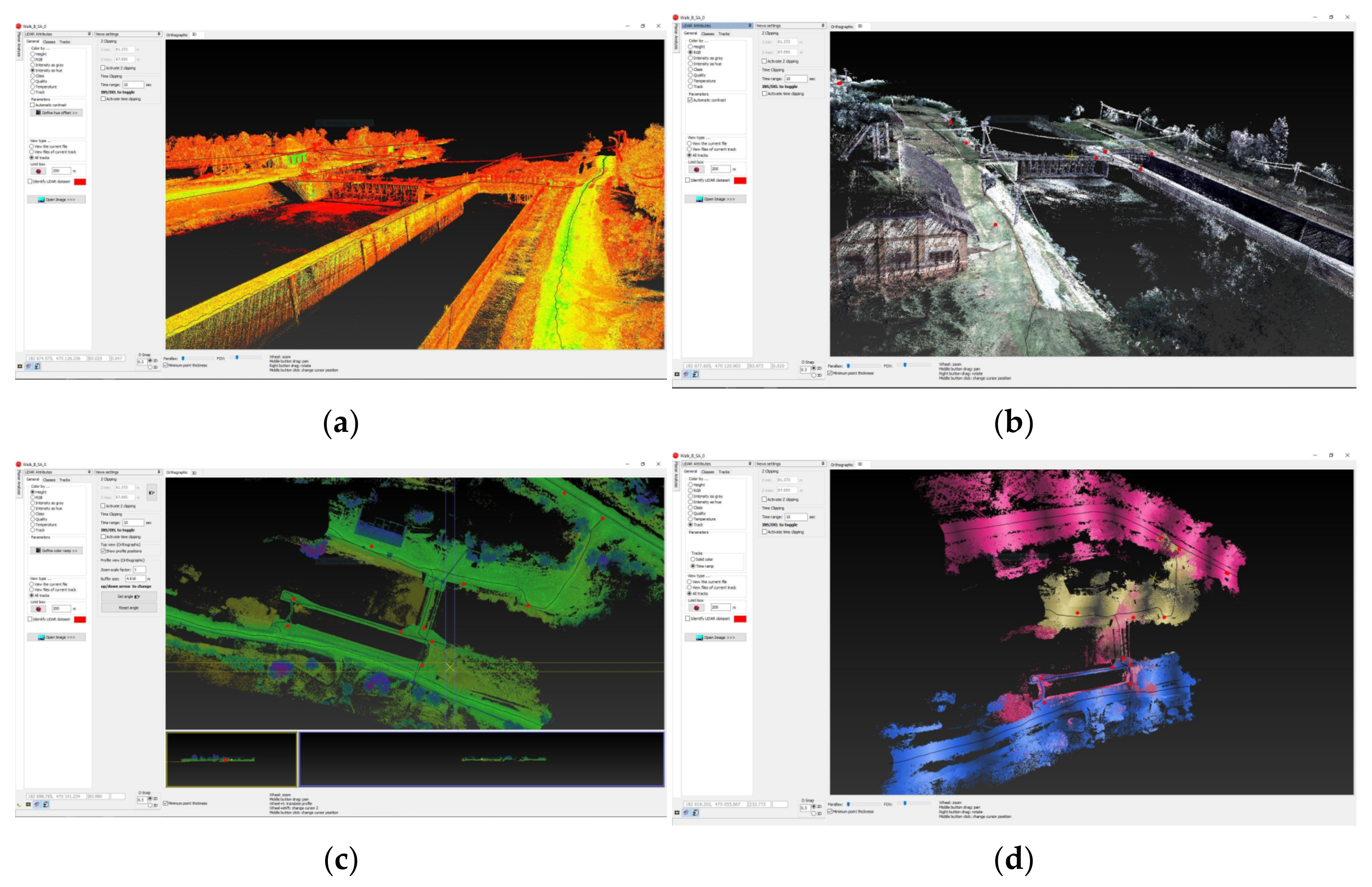
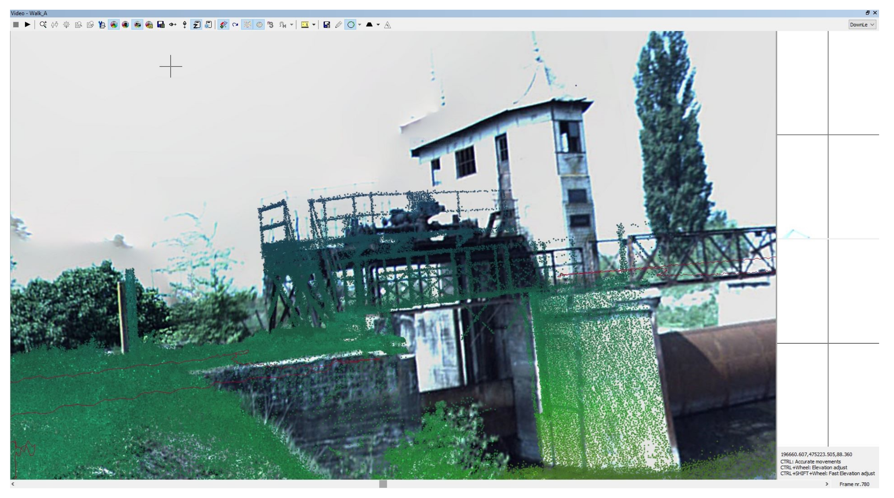
3.4.2. Data Processing in Pegasus Manager and Obtaining Point Clouds

The processing of LiDAR data (Figure 30), collected with the help of Leica Pegasus Backpack equipment, is carried out with the help of the Pegasus Manager program, and includes several steps https://www.mdpi.com/2073-4441/12/10/2895 (accessed on 1 October 2022).

In Figure 31a–d one may notice the intensity of the nuance of the LiDAR data, the coloring per height and RGB coloring for H NCoșteiu, which was performed on 15 May 2019.

Figure 32a–d also show the LiDAR point clouds according to the intensity, the coloring according to the Walks (i.e., how many subprojects were made within a scanning project) and the RGB visualization of the point clouds, where each LiDAR point is colored according to the color of the corresponding pixel from the images taken during the scan for the Cruceni Pumping Station, a scan performed on 3 June 2019. On 23 July 2019, the scanning of the Lock from Sânmartinu Maghiar was also performed, and this is represented in the work by Figure 33a–d.

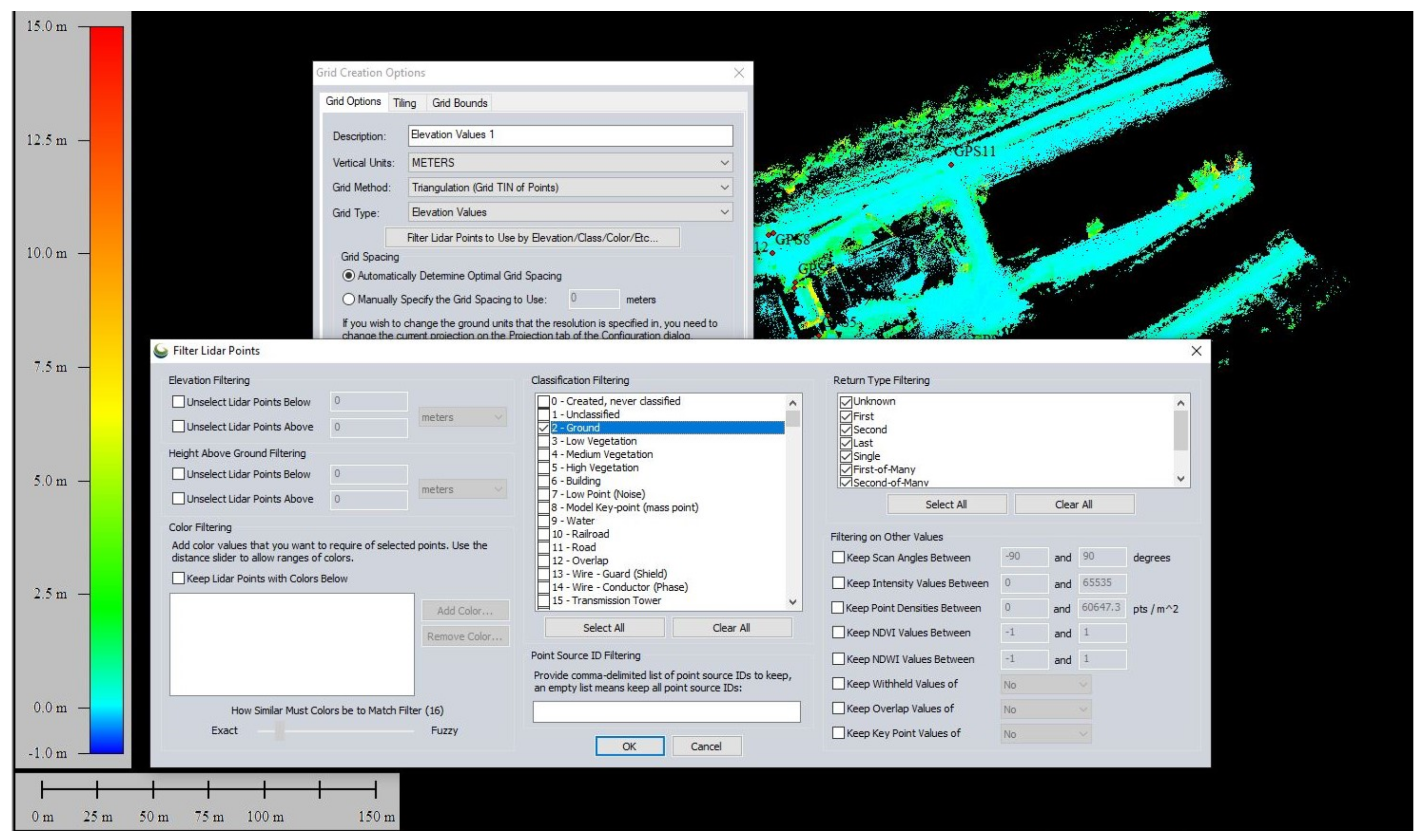
3.4.3. LiDAR Data Processing in ArcGIS—Leica Pegasus: MapFactory

The results obtained from data processing will be further processed with the GIS program using the MapFactory module which is an ArcGIS module of work used from data collection to final extraction.

MapFactory programs for GIS, MapFactory for AutoCAD, and Cyclone with CloudWorx module and 3D modeling module (Cyclone model) allow viewing images and clouds of LiDAR points (Figure 34), to analyze, collect, and export LiDAR data. After the objects have been measured and meta-labeled, the data can be exported in different formats, including AutoCAD.

Also the clouds of LiDAR points obtained from the scanning of the Coșteiu Hydrotechnical Node, of the Sânmihaiu Român and Sânmartinu Maghiar Locks, as well as of the Cruceni Pumping Station, using the MMS scanning technology with the Leica Pegasus Backpack in the Pegasus Manager program, they were exported to a LiDAR file of type LAS and E57 and later on imported into the Cyclone Model program from Leica where, through CloudWorx mode for AutoCAD Map and the 3D modeling mode used, allows viewing the digital reality in CAD and achieving the 3D situation plan of the hydrotechnical objectives. This CloudWorx module uses the Cyclone program as a working platform and as a basis for viewing point clouds. Thus, LiDAR points can be viewed, analyzed, vectorized, and exported to CAD.

It automatically recognizes the change in the road level. The deformation is classified according to the colored height—thus, a quick recognition of the extent of the deformation is allowed (Figure 35).

3.5. Comparison of TLS—MMS Data

If in the case of engineering photogrammetry the point clouds are obtained from the aerial images collected with the drone (Phantom 4 Pro), in the case of MMS mobile scanning technology, where we used a Leica Pegasus backpack, point clouds are obtained from the two Velodyne scanning systems [20], each provided with 16 LiDAR data retrieval lasers (LiDAR SO + LiDAR SA), with an amazing accuracy of a few millimeters, and the images obtained from the 5 cameras will be used to color the LiDAR points, from the raw shape, which have flashy colors of red, yellow, and green in a real form, where each LiDAR point will color based on the pixels in the images, in fraction of a second.

The same happened with the use of TLS terrestrial scanning technology, where a Leica ScanStation C10 equipment was used to scan hydrotechnical objectives, with the following clear differences (

Table 17. Comparison of TLS—MMS scanning systems.

Features	Scanning Equipment
	ScanStation Leica C10	Leica Pegasus
Number of points	50,000 points/s	600,000 points/s
Cameras	1 camera	5 rooms
Gyroscope	No, being static	Yes
Accelerometer	No, being static	Yes
GNSS	No	Yes
GRID choice	Yes (from 1m—mx cm)	No (it’s according to the speed)
Data collection time	Long allotted time/station, requiring knowledge for the implementation and orientation of topographical instruments	Short time, being mobile, does not require targets and knowledge of placing topographic equipment in the station
Processing time	Quite short, knowledge for automatic and manual alignment of points	Long, SLAM processing, Kalman Filter
Number of images	260/station	Depending on the chosen distance, which will be multiplied by 5 (5 cameras)
Preparation of the gear	Time identical to the placement of a total station	It involves mounting a GNSS reference station, a dynamic initialization and a static one, and after the scans are completed, the repetition of the two initializations
Use targets	Yes	No
Ground control points (GCP)	No	Yes
Weight	16 kg	11.9 kg
Battery life	Long, with the possibility of change while performing the scan, scans with 2 batteries at a time, and automatic permutation between them	Long, scans with 4 batteries at once, and with automatic permutation between them, first the top two will be consumed, then the bottom two
Scanning angle	360 degrees in the horizontal plane with 270 degrees in the vertical plane	360 degrees horizontally with 200 degrees in the vertical plane
Scanning temperature	Greater than 4 °C, or possibly a “jacket” will be purchased for the device, avoiding places with strong and cold winds	Below 0 °C, because the mechanism is covered, scanning is also possible in windy and cold conditions
Other optional items	The need to make black & white targets for each work, or to purchase 6-inch targets from suppliers	A GNSS equipment for RiNNEX data collection, installation of a reference station

).

3.6. Comparing UAV-TLS-MMS Data

In the case of UAV equipment, due to the fact that the data is recorded from a height, they face difficulties in obtaining information about objects from the ground, for example under trees and along the facades of the buildings. On the contrary, MMS collects high-precision point clouds from the ground along with stereographic images but lacks information about the top. For example, a roof. In case of errors, due to the lack of the GNSS signal or when it is weak, it will be intervened to correct it by compensating the time, meaning that it will be compensated the time during which the Leica Pegasus backpack was left without a good signal to the GNSS, or not at all, through the SLAM function and the Kalman filter.

In the table below you can see some parameters compared between DJI Phantom 4 Pro GNSS RTK [57], Leica ScanStation C10 and Leica Pegasus Backpack (

Table 18. Comparisons between UAV, TLS and MMS equipment.

Features	DJI Phantom 4 Pro GNSS RTK-UAV	Leica ScanStation C10_TLS	Leica Pegasus Backpack_MMS
Control network	A lot of needs	A lot of needs	Just a few needed if GNSS visibility is poor
Regulations	Strict regulations, especially in urban areas	No	No
Inside/outside	Exterior only	Interior & Exterior	Interior & Exterior
Data collection time	Reduced	Larger	Reduced
Data processing time	Fast	Medium	Elevated
Absolute accuracy in 3D	5.0 to 8.0 cm	0.1 to 1.0 cm	2–4 cm
Flexibility	Average (due to strict regulations)	High	High
Cost	Medium	Reduced	Elevated
Price in Euro	≈1500	≈80,000	≈400,000

).

This paper focuses on the integration of UAV images and LiDAR point clouds-MMS and TLS to build high-resolution 3D models for hydrotechnical objectives and realization a data visualization link using the Leica TruView program, thus creating a digital world.

Table 19. Comparative data for several devices using mobile scanning technology.

Manufacturer	Leica Pegasus: Backpack	Viametris BMS3D	OSLAM	HERON	Li-Backpack	ROBIN 3DLM–Walk Drive Fly
Spherical images	200°–5 cam–20 MPIX	360°–LB5:30 MPIX or 4cam 200°–20 MPIX	360°–LB5: 30 MPIX	360°–2 MPIX	N O	y 70°–5 MPIX
Photogrammetry	YES	NO	NO	NO	NO	NO
Scanner	VLP16	VLP16	VLP16	VLP16	VLP16	NO
GNSS	High-precision GNSS antenna	GNSS Antenna	GNSS Antenna	NO	NO	2 GNSS antennas
IMU	IMU High, 125 HZ	NO	NO	NO	NO	YES
SLAM	YES	YES	YES	YES	YES	YES with the help of an additional ZEBREVO device
Flashlight/ lantern	YES	NO	NO	NO	NO	NO
Positioning	GNSS/IMU/SLAM/RTK	SLAM/GNSS	SLAM/GNSS	SLAM	SLAM	GNSS/IMU/SLAM
Ergonomics	Perfectly wearable, it is up to the level of the head, there is no danger of hitting the door frame for example (REDDOT award for design)	It is not perfectly wearable, the antenna arm poses a danger of hitting the door frame, it is overhead	It is not perfectly wearable, the antenna arm poses a danger of hitting the door frame, it is overhead	Danger of hitting the height	Danger of hitting the height	Difficult to wear for more than 45 min because it has 2 antennas, the center of gravity is not suitable

shows comparative data made between several mobile scanning equipment, equipment that was the subject of the research, before purchasing the equipment from Leica, the Pegasus Backpack model.

In the

Table 20. Comparing data on mobile scanning systems (MMS).

Producer/Distributor	Vexcel	Leica
Country	Austria	Switzerland
points/second	300,000	600,000
field of view	26 cameras 360 oriz/30 vert. 6,6 MP	360 oriz/200 vert.
Camera	1 camera 360 roiz/180 vert 105 mp	5 cameras × 4 MP CCD + 2 LiDAR sensors
CCD	2088 × 2152	2046 × 2046
pixel size	1.4 × 1.4 microns	5.5 × 5.5 microns
Lens	3.24 mm focal length	6 mm focal length
Max. frame speed/second	1.5 fps	2 fps
data type	LiDAR	LiDAR
3D laser scanner	Rotating multi-beam LiDAR	Dual Velodyne VLP16 with 270 × 30 aperture to scanner
No. of channels	16	16
Frequency	10 Hz	10 Hz
working distance	100 m	100 m is maximum, useful is 70 m
Batteries	2 batteries up to 2 h of work	4 batteries up to 6 h of work
positioning system	GNSS/IMU	GNSS/IMU (Clear Navigation Unit for mapping in locations without GNSS/SLAM signal (Simultaneus Localisation And Mapping) for mapping and localization
Constellations	-	GPS, GLONASS, GALILEO, BEI DU
Band	Multiband GNSS	L-band, SBAS, QZSS
software included	Ultra-Essential Terrestrial Map	Infinity Basic
Temperature	0–40 degrees C	0–40 degrees C
storage temp.	−20 to + 50	from −20 to + 50
	-	1GB/minute of travel
weight	16.0 kg	11.9 kg
Dimensions	110 × 37 × 32	73 × 27 × 31
Relative	3 cm	2–3 cm outside/inside
absolute on the outside	5 cm	5 cm
absolute on the inside without checkpoints	-	5–50 cm for 10 min walking, minimum 3 double passes
Images	JPG, TIFF	JPG, ASCII for photogrammetric parameters
point clouds	LAS	LAS, RGB, Recap, 2D, 3D, E57, DWG, DGN, KMZ

can see similarities and differences in the way of data collection, accuracy of cameras, batteries, weight, etc.

4. Conclusions

This scientific paper reports the current state of research in the field of UAV, TLS, and MMS for geomatic and hydrological applications, providing an overview of different platforms, applications, and case studies with the help of a Drone Phantom 4 Pro. This paper also presents the latest developments in UAV image processing. At the same time, the technique of using UAV platforms is correlated with the TLS (Terrestrial Laser Scanners) technique, using a Leica ScanStation C10 scanner together with the mobile scanning technique (MMS—Mobile Mapping System), the Leica Pegasus Backpack, for the 3D scanning of hydrotechnical and hydro-ameliorative lenses [58].

Through this paper, scientific research was carried out, which was necessary to create a database through terrestrial (fixed and mobile) and aerial 3D laser scans of the objectives taken in the study (the hydrotechnical nodes from Topolovăţu Mic and Coșteiu, Sânmartinu Maghiar, as well as the Cruceni pumping station).

The georeference error in the case of using the control points (GCP) and checking them in AutoCAD was between 2–4 cm for the hydrotechnical objectives studied, namely NH Topolovăţu Mic, NH Coşteiu, HN Sânmihaiu Român, Sânmartinu Maghiar Lock and Cruceni Pumping Station.

By comparing with the traditional methods using classical tools, data collection is difficult or even impossible to be acquired but using the laser scanning method we will obtain accurate investigation data in a short time and with multiple possibilities of processing and viewing point clouds.

By using the Cyclone Model program used for data processing, the topographical elements of the land could be easily extracted in order to make a numerical model of the land, process the facades of the constructions, realize the situation plans, and make the transverse and longitudinal profiles; in the end, we obtained information on the X, Y, Z values of the points, as well as the realization of a virtual flight on the scanned objective or of a virtual tour where we also had information about the clouds of points, distances and also the creation at the end of a ‘link’ that can be transmitted further to the interested units and the import of this data on the website so that it can be accessed by anyone.

Due to continuous developments in both scanning and navigation technologies, the landscape of mobile mapping systems varies and is evolving rapidly. Consequently, we have produced a comparative table that offers a review of the main current commercial systems available on the market (

Table 21. The most common common commercial mobile cartography systems and related components post-processed precision data values such as RMS.

Provider	Name	Laser Scanner			IMU/GNSS	Digital Camera
		Sensor (s)	Range	Accuracy	Pos. Absolute	Resolution
TOPCON	IP-S3	1 scanner	100 m, @ ρ100%	50 mm@ 10 m (1σ)	0.015–0.025 m	Spherical camera, 8000 × 4000 px
TRIMBLE	MX8	1-2 VQ-250	500 m, @ ρ80%	10 mm@ 50 m (1σ)	0.020–0.025 m	Up to 7 cameras, 5 Mpx
		1-2 VQ-450	800 m, @ ρ80%	8 mm@ 50 m (1σ)
3D laser mapping	Street Mapper	1-2 VUX-1HA	400 m, @ ρ80%	5 mm, (1σ)	0.050 m	Panoramic camera, 12 Mpx
Riegl	VMX-250	2 VQ-250	500 m, @ ρ80%	10 mm@ 50 m (1σ)	0.020–0.050 m	Up to 6 cameras, 5 Mpx
renishaw	Dynascan S250	1-2 scanner(s)	250 m	10 mm@ 50 m (1σ)	0.020–0.050 m	-
TELEDYNE OPTECH	Lynx SG1	2 scanners	250 m, @ ρ10%	5 mm, (1σ)	0.050 m	Up to 5 cameras, 5 Mpx and/or panoramic camera
	Lynx MG1	1 scanner			0.200 m
Leica Geosystems	Leica Pegasus	ZF 9012	119 m	0.9 mm@ 50 m, ρ80% (1σ)	0.015–0.020 m	8 cameras, 2000 × 2000 px
		Leica P20 scan	120 m, @ ρ18%	6 mm@ 100 m (1σ)

).

The RADMIN program helped to achieve the calibration of the images, the realization of the project and also provided important data during the scans regarding, the scanning speed (m/s), the INS value, the number of satellites at the time of scanning.

All this presented data finally led to a scan with high precision, resulting at the end of data processing and application of the Kalman filter into a cloud of points with an accuracy of 1–3 cm, accuracy which was verified with the help of the resulting stereographic images, where the positioning accuracy of the point clouds were improved when used ground control points (GCP). These ground control points (GCP) had the role of verification and control as well as in the processing of point clouds.

As part of the research carried out for the elaboration of this scientific paper, LAS data type was imported and processed using Cyclone, Global Mapper [59], 3D Resheaper and CloudCompare [60] programs and the file with the E57 extension, thanks to the new version from Cyclone Model, version 9.3, processed data could be imported directly into Cyclone Model due to the new option of ‘Import data from Leica Pegasus’.

Estimated errors for the scanned lenses in this work are characterized by an average dispersion of ± 5.7 cm (MMS vs. UAV) and ± 1.6–2 cm (MMS vs. TLS) [61].

The combinations for the Kalman Filter for guidance, navigation and control decreased from 55 to just 6 combinations, thus reducing the post-processing time [62].

With the help of modern 3D scanners, it is possible to successfully track in time the constructions, respectively of the natural or artificial hydrotechnical dams and to obtain 3D data in real time with the possibility of quick evaluation and decision-making, where the most accurate data and with the smallest errors were obtained with the 3D scanning equipment, the Leica C10 model comparing to the Leica Pegasus Backpack equipment.

UAV technology can be used mainly for monitoring slopes, landslides, soil erosion monitoring or farm monitoring.

In conclusion, the measurements made with the ScanStation Leica C10 equipment, require longer time with stages similar to the use of a total station, but with amazing results, with high accuracies of the order of millimeters, 0–6 mm, while the use of the Leica Pegasus Backpack backpack requires a very short time to perform scans, which also involves the installation of a reference for RiNNEX data collection, which can be performed, by walking or from a car, with a maximum speed of 20 km/h, where the obtained accuracies are of the order of centimeters, 1–3 cm, resulting in a volume large of raw data, where after carrying out the processing and obtaining the clouds of points these final data will be 5–6 times higher.

The Bega Canal was arranged 250 years ago, and from a hydrotechnical point of view, it is a building with special arrangements, which presents a significant importance from a historical and architectural point of view. The Timișoara—Klek waterway has a total length of 114.50 km, of which on the Romanian territory about 44.5 km and the Serbian territory of 70 km.

The navigable sector of the Bega Canal on the territory of the Republic of Serbia, is connected with the Danube-Tisza-Danube hydroameliorative and navigation system. The Bega Canal is one of the significant waterways for Zrenjanin, Zitiste and Timișoara; its relaunch in terms of navigation would mean the connection of Banat, both to the Black Sea and to the North Sea, the existing system of canals from Serbia DTD (Danube—Tisza—Danube) and the Rhine-Main–Danube Channel.

By repairing the Sânmihaiu Român, Srpski Itebej and Klek hydrotechnical hubs, the connection of the bicycle route on the Romanian side with the one on the Serbian sector will be made, thus also making a connection between Timisoara and Zrenjanin along the Bega Canal and defending much wider opportunities for commercial and economic cooperation. Such a project will result in the creation and development of transport links on both sides of the border, as well as the promotion of good neighbourliness and cooperation between Romania and Serbia.

Currently, these activities are in progress, and in August 2021 the Bega became navigable. Following the implementation and completion of the project, a new border crossing point with Serbia will also be arranged through the point/place where the Bega leaves the country. The steps have already been taken, and through the canal system in Serbia, Timisoara will be again connected to the Danube and then to the North Sea [63].

Supplementing the results obtained with the help of modern 3D scanning technologies with photogrammetric results are necessary where these technologies complement each other and are not excluded.

The data presented in this scientific paper are original and were made in the period 2017–2020 and constitutes the future for obtaining data in a short time and of good quality through the possibility of comparing the results and by using the ground control points (GCP) on a mandatory basis.

References

1. Resop, J.P.; Lehmann, L.; Hession, W.C. Drone Laser Scanning for Modeling Riverscape Topography and Vegetation: Comparison with Traditional Aerial LiDAR. Drones 2019, 3, 35. [Google Scholar] [CrossRef] [Green Version]
2. Mielcarek, M.; Kamińska, A.; Stereńczak, K. Digital Aerial Photogrammetry (DAP) and Airborne Laser Scanning (ALS) as Sources of Information about Tree Height: Comparisons of the Accuracy of Remote Sensing Methods for Tree Height Estimation. Remote Sens. 2020, 12, 1808. [Google Scholar] [CrossRef]
3. Beilicci, E.; David, I.; Beilicci, R.; Visescu, M. Mathematical model for calculation of soil loss on watershed slopes. Environ. Eng. Manag. J. 2017, 16, 2211–2218. [Google Scholar] [CrossRef]
4. Iordan, D. The Application of Laser Technologies to the Topographic Stage of the Someș-Tisa Hydrographic Basin. Ph.D. Thesis, University of Bucharest, Bucharest, Romania, 2014; p. 1. [Google Scholar]
5. Available online: https://www.ghd.com/en/perspectives/how-3d-laser-scanning-is-changing-the-engineering-landscape.aspx (accessed on 15 May 2021).
6. Gerald, F.M. Handbook of Optical and Laser Scanning; Marcel Dekker, University of Rochester, Inc.: New York, NY, USA, 2004. [Google Scholar]
7. Ebrahim, M.A.B. 3D Laser Scanners: History, Applications and Future. Ph.D. Thesis, Faculty of Enginnering Assiut University, Asyut, Egypt, 2011. [Google Scholar]
8. Savu, A.; Caius, D.; Cornelia, B.A.; Gheorghe, B. Laser Scanning Airborne Systems—A New Step in Engineering Surveying. In Proceedings of the 11th WSEAS International Conference on Sustainability in Science Engineering SSE, Timisoara, Romania, 27–29 May 2009; Volume 9, pp. 27–29. [Google Scholar]
9. Qiu, Q.; Wang, M.; Xie, Q.; Han, J.; Zhou, X. Extracting 3D Indoor Maps with Any Shape Accurately Using Building Information Modeling Data. ISPRS Int. J. Geo-Inf. 2021, 10, 700. [Google Scholar] [CrossRef]
10. De Antero, K.; Kaartinen, H.; Virtanen, J.P. Laser Scanner in a Backpack; GIM International: Masala, Finland, 2016; Volume 30, pp. 16–19. [Google Scholar]
11. Riley, P.; Crowe, P. Airborne and Terrestrial Laser Scanning—Applications for Illawarra Coal. In Proceedings of the Coal Operators’ Conference, Wollongong, Australia, 18–20 February 2006; pp. 266–275. [Google Scholar]
12. Abdelhafiz, A. Integrating Digital Photogrammetry and Terrestrial Laser Scanning. Ph.D Thesis, Braunschweig, Technischen Universität Braunschweig, Braunschweig, Germany, 2009. ISBN 3-926146-18-4. [Google Scholar]
13. Di Stefano, F.; Chiappini, S.; Gorreja, A.; Balestra, M.; Pierdicca, R. Mobile 3D scan LiDAR: A literature review. Geomat. Nat. Hazards Risk 2021, 12, 2387–2429. [Google Scholar] [CrossRef]
14. Smits, J.; Confalone, G.; Kinnare, T. What Is the Difference between Laser Radar and LiDAR Technology? ECM, Global Measurament Solution: Topsfield, MA, USA, 2022. [Google Scholar]
15. Rusu, G.; Herban, I.S.; Bălă, A.C.; Grecea, C. Mathematical support for three-dimensional transformation points from geocentric reference system in local reference system. AIP Conf. Proc. 2015, 1648, 670011. [Google Scholar]
16. Kwan, M.P.; Ransberger, D.M. LiDAR assisted emergency response: Detection of transport network obstructions caused by major disasters. Comput. Environ. Urban Sys. 2010, 34, 179–188. [Google Scholar] [CrossRef]
17. Hol, J. Sensor Fusion and Calibration of Inertial Sensors, Vision, UltraWideband and GPS. Linköping Studies in Science and Technology. Ph.D. Thesis, Linköping University, Linköping, Sweden, 2011. [Google Scholar]
18. Strasdat, H.; Montiel, J.M.M.; Davison, A.J. Real-time monocular SLAM: Why filter? In Proceedings of the IEEE International Conference on Robotics and Automation, Anchorage, AK, USA, 3–7 May 2010. [Google Scholar]
19. Tardif, J.P.; George, M.; Laverne, M. A new approach to vision-aided inertial navigation. In Proceedings of the IEEE/RSJ International Conference, Intelligent Robots and Systems (IROS), Taipei, Taiwan, 18–22 October 2010. [Google Scholar]
20. Velodyne. The Velodyne High Definition LiDAR; Velodyne: San Jose, CA, USA, 2014. [Google Scholar]
21. Leica Pegasus Backpack Technical Sheet. Available online: http://www.topgeocart.ro/platforme-mobile/leica-pegasusbackpack_97.html (accessed on 5 June 2022).
22. Thrun, S.; Leonard, J.J. Simultaneous Localization and Mapping. In Siciliano, B., Khatib, O. Handbook of Robotics; Springer: Berlin/Heidelberg, Germany, 2008. [Google Scholar] [CrossRef] [Green Version]
23. Grecea, C.; Herban, I.S.; Vilceanu, C.B. WebGIS solution for urban planning strategies. Procedia Eng. 2016, 161, 1625–1630. [Google Scholar] [CrossRef] [Green Version]
24. Lo Bruto, M.; Borruso, A.; D’Argenio, A. UAV System for photogrammetric data acquisition of archeological sites. Int. J. Herit. Digit. Era 2012, 1, 7–13. [Google Scholar] [CrossRef] [Green Version]
25. Li, J.; Knapp, D.E.; Lyons, M.; Roelfsema, C.; Phinn, S.; Schill, S.R.; Asner, G.P. Automated Global Shallow Water Bathymetry Mapping Using Google Earth Engine. Remote Sens. 2021, 13, 1469. [Google Scholar] [CrossRef]
26. Șmuleac, A.; Șmuleac, L.; Man, T.E.; Popescu, C.A.; Imbrea, F.; Radulov, I.; Adamov, T.; Pașcalău, R. Use of Modern Technologies for the Conservation of Historical Heritage in Water Management. Water 2020, 12, 2895. [Google Scholar] [CrossRef]
27. Dunea, D.; Bretcan, P.; Tanislav, D.; Serban, G.; Teodorescu, R.; Iordache, S.; Petrescu, N.; Tuchiu, E. Evaluation of Water Quality in Ialomita River Basin in Relationship with Land Cover Patterns. Water 2020, 12, 735. [Google Scholar] [CrossRef] [Green Version]
28. Burghelea, B.; Bănăduc, D.; Bănăduc, A. The Timiş River Basin (Banat, Romania) Natural and Anthropogenic Elements. A Study Case—Management Chalenges. Transylv. Rev. Syst. Ecol. Res. 2013, 15, 173–206. [Google Scholar] [CrossRef]
29. Tommaselli, A.M.G.; Moraes, M.V.A.; Silva, L.S.L.; Rubio, M.F.; Carvalho, G.J.; Tommaselli, J.T.G. Monitoring marginal erosion in hydroelectric reservoirs with terrestrial mobile Laser scanner. Int. Arch. Photogramm. Remote Sens. Spat. Inf. Sci. XL 2014, 5, 589–596. [Google Scholar] [CrossRef] [Green Version]
30. Şmuleac, L.; Rujescu, C.; Șmuleac, A.; Imbrea, F.; Radulov, I.; Manea, D.; Ienciu, A.; Adamov, T.; Pașcalău, R. Impact of Climate Change in the Banat Plain, Western Romania, on the Accessibility of Water for Crop Production in Agriculture. Agriculture 2020, 10, 437. [Google Scholar] [CrossRef]
31. Micek, O.; Feranec, J.; Stych, P. Land Use/Land Cover Data of the Urban Atlas and the Cadastre of Real Estate: An Evaluation Study in the Prague Metropolitan Region. Land 2020, 9, 153. [Google Scholar] [CrossRef]
32. Bilașco, Ș.; Roșca, S.; Vescan, I.; Fodorean, I.; Dohotar, V.; Sestras, P. A GIS-Based Spatial Analysis Model Approach for Identification of Optimal Hydrotechnical Solutions for Gully Erosion Stabilization. Case Study. Appl. Sci. 2021, 11, 4847. [Google Scholar] [CrossRef]
33. IWA Publishing. Water Supply; IWA Publishing: London, UK, 2022. [Google Scholar]
34. Depetris, P.J. The Importance of Monitoring River Water Discharge, Frontiers in Water. Front. Water 2021, 3, 745912. [Google Scholar] [CrossRef]
35. Drăghici, I.A.; Rus, I.D.; Cococeanu, A.; Muntean, S. Improved Operation Strategy of the Pumping System Implemented in Timisoara Municipal Water Treatment Station. Sustainability 2022, 14, 9130. [Google Scholar] [CrossRef]
36. Radutu, A.; Luca, O.; Gogu, C.R. Groundwater and Urban Planning Perspective. Water 2022, 14, 1627. [Google Scholar] [CrossRef]
37. Olaru, M. A history of about 300 years of high waters and hydrotechnic constructions in Banat (I). Rev. Hist. Geogr. Toponomast. 2006, I, 89–106. [Google Scholar]
38. Tyszewska, P.D. Water Management Balance as a Tool for Analysis of a River Basin with Conflicting Environmental and Navigational Water Demands: An Example of the Warta Mouth National Park, Poland. Water 2021, 13, 3628. [Google Scholar] [CrossRef]
39. Oniga, V.E.; Breaban, A.I.; Pfeifer, N.; Diac, M. 3D Modeling of Urban Area Based on Oblique UAS Images—An End-to-End Pipeline. Remote Sens. 2022, 14, 422. [Google Scholar] [CrossRef]
40. Skrzypczak, I.; Kokoszka, W.; Zientek, D.; Tang, Y.; Kogut, J. Landslide Hazard Assessment Map as an Element Supporting Spatial Planning: The Flysch Carpathians Region Study. Remote Sens. 2021, 13, 317. [Google Scholar] [CrossRef]
41. Paudel, S.; Benjankar, R. Integrated Hydrological Modeling to Analyze the Effects of Precipitation on Surface Water and Groundwater Hydrologic Processes in a Small Watershed. Hydrology 2022, 9, 37. [Google Scholar] [CrossRef]
42. Man, T.E.; Blenesi, D.A.; Constantinescu, L. Technical solutions to create esthetical civil engineering structures using the geosynthetics materials. Ann. Food Sci. Technol. 2010, 11, 111–117. [Google Scholar]
43. Salmoral, G.; Rivas Casado, M.; Muthusamy, M.; Butler, D.; Menon, P.P.; Leinster, P. Guidelines for the Use of Unmanned Aerial Systems in Flood Emergency Response. Water 2020, 12, 521. [Google Scholar] [CrossRef] [Green Version]
44. Man, T.E.; Armas, A.; Beilicci, R.; Beilicci, E. Assessment Regarding the Evolution in Time (1980–2014) of Drought on the Basis of Several Computation Indexes: Study Case Timisoara. Nat. Resour. Sustain. Dev. 2018, 8. [Google Scholar] [CrossRef]
45. Dunca, A.M. Water Resources in the Timiş-Bega Hydrographic System: Genesis, Hydrological Regime and Water Risks; Editura Universităţii de Vest: Timisoara, Romania, 2016; ISBN 978-973-125-519-4. [Google Scholar]
46. Cioffi, F.; De Bonis Trapella, A.; Giannini, M.; Lall, U. A Flood Risk Management Model to Identify Optimal Defence Policies in Coastal Areas Considering Uncertainties in Climate Projections. Water 2022, 14, 1481. [Google Scholar] [CrossRef]
47. Khan, M.Y.A.; ElKashouty, M.; Subyani, A.M.; Tian, F. Flash Flood Assessment and Management for Sustainable Development Using Geospatial Technology and WMS Models in Abha City, Aseer Region, Saudi Arabia. Sustainability 2022, 14, 10430. [Google Scholar] [CrossRef]
48. Available online: https://en.unesco.org/themes/water-security/hydrology/programmes/whymap (accessed on 3 February 2021).
49. Elhashash, M.; Albanwan, H.; Qin, R. A Review of Mobile Mapping Systems: From Sensors to Applications. Sensors 2022, 22, 4262. [Google Scholar] [CrossRef]
50. TransDatRO. Available online: https://cngcft.ro/index.php/ro/download (accessed on 13 July 2022).
51. Remondino, F.; Spera, M.G.; Nocerino, E.; Menna, F.; Nex, F. State of the art in high density image matching. Photogramm. Rec. 2014, 29, 144–166. [Google Scholar] [CrossRef]
52. Yu, J.J.; Kim, D.W.; Lee, E.J.; Son, S.W. Determining the Optimal Number of Ground Control Points for Varying Study Sites through Accuracy Evaluation of Unmanned Aerial System-Based 3D Point Clouds and Digital Surface Models. Drones 2020, 4, 49. [Google Scholar] [CrossRef]
53. Elkhrachy, I. 3D Structure from 2D Dimensional Images Using Structure from Motion Algorithms. Sustainability 2022, 14, 5399. [Google Scholar] [CrossRef]
54. Herban, I.S.; Rusu, G.; Grecea, O.; Birla, G.A. Using the laser scanning for research and conservation of cultural heritage sites. Case study: Ulmetum Citadel. J. Environ. Prot. Ecol. 2014, 15, 1172–1180. [Google Scholar]
55. Calin, M.; Damian, G.; Popescu, T.; Manea, R.; Erghelegiu, B.; Salagean, T. 3D Modeling for Digital Preservation of Romanian Heritage Monuments. Agric. Agric. Sci. Procedia 2015, 6, 421–428. [Google Scholar] [CrossRef] [Green Version]
56. Zhao, L.; Li, N.; Li, L.; Zhang, Y.; Cheng, C. Real-Time GNSS-Based Attitude Determination in the Measurement Domain. Sensors 2017, 17, 296. [Google Scholar] [CrossRef]
57. Available online: https://store.dji.com/product/phantom-4-pro (accessed on 25 March 2021).
58. Available online: https://novatel.com (accessed on 12 December 2020).
59. Global Mapper v.20; Blue Marble, Maine, USA, Geographics. Available online: https://www.bluemarblegeo.com/global-mapper/ (accessed on 18 November 2020).
60. CloudCompare 3D Point Cloud and Mesh Processing Software; Open Source. Available online: http://www.cloudcompare.org/ (accessed on 3 October 2020).
61. Available online: https://leica-geosystems.com/products/mobile-mapping-systems/capture-platforms/leica-pegasus-backpack (accessed on 12 December 2021).
62. Available online: https://rentals.leica-geosystems.com/support/7AAAF268-5056-8236-9A2F67975423FC85.pdf (accessed on 25 December 2021).
63. Available online: http://expertconsulting.ro/the-repairing-of-navigation-infrastructure-on-bega-canal/ (accessed on 23 July 2022).
Figure 1. Leica Pegasus equipment (https://leica-geosystems.com/ (accessed on 12 December 2021).
Water 14 03729 g001
Figure 2. Planning the flight in the study area, with the indication of the flight bands followed by the UAV.
Water 14 03729 g002
Figure 3. Mission type.
Water 14 03729 g003
Figure 4. Fused SLAM Acquisition.
Water 14 03729 g004
Figure 5. Initialization of the MMS equipment.
Water 14 03729 g005
Figure 6. Rinex data collection at one second ( Pumping Station, Cruceni, Romania).
Water 14 03729 g006
Figure 7. Presentation of the checkpoints and trajectory for the scanned objectives.
Water 14 03729 g007
Figure 8. Timiș-Bega interconnection—synoptic scheme (A.B.A. Banat).
Water 14 03729 g008
Figure 9. Planning measurements: (a) Chart of GDOP Values Topolovăţu Mic; (b) Constellation and trajectory of the satellites for Topolovăţu Mic.
Water 14 03729 g009
Figure 10. Height of satellites.
Water 14 03729 g010
Figure 11. Presentation of errors for the measurements performed.
Water 14 03729 g011
Figure 12. Alignment of images: (a) session I-a; (b) session II-a.
Water 14 03729 g012
Figure 13. DSM generated by photogrammetric technique.
Water 14 03729 g013
Figure 14. Orthophotoplan obtained by aerial data processing, Topolovăţu Mic, Timiș, Romania.
Water 14 03729 g014
Figure 15. Orthophotoplan obtained by processing aerial data: (a) Ortophotoplan ANCPI—2015 (Topolovăţu Mic, Timiș, Romania); (b) Ortopotoplan UAV—2018 (Topolovăţu Mic Hydrotechnical Node, Timiș, Romania).
Water 14 03729 g015
Figure 16. Point Cloud-NH Coșteiu.
Water 14 03729 g016
Figure 17. Point Cloud-Sânmihaiu Român Lock.
Water 14 03729 g017
Figure 18. Point Cloud-Sânmartinu Maghiar Lock.
Water 14 03729 g018
Figure 19. Point Cloud-Cruceni Pumping Station.
Water 14 03729 g019
Figure 20. TruView link for NH Coșteiu.
Water 14 03729 g020
Figure 21. TruView link for NH Topolovăţu Mic.
Water 14 03729 g021
Figure 22. TruView link for the Lock from Sânmihaiu Român.
Water 14 03729 g022
Figure 23. TruView link for the Lock from Sânmartinu Maghiar.
Water 14 03729 g023
Figure 24. TruView link for Cruceni Pumping Station.
Water 14 03729 g024
Figure 25. View option in Inertial Explorer (IE).
Water 14 03729 g025
Figure 26. 3D scanning of the HN Coșteiu—Museum lens on: 13.05.2019: (a) View of scan accuracy (Combined separation); (b) The number of visible satellites at the time of the scan; (c) RMS values; (d) PDOP values.
Water 14 03729 g026
Figure 27. 3D scanning of the objective NH Costeiu–Dam on 15.05.2019: (a) View of scan accuracy (Combined separation); (b) The number of visible satellites at the time of the scan; (c) RMS values; (d) Estimation of data accuracy (X, Y, Z and Time).
Water 14 03729 g027
Figure 28. 3D scanning of the objective CRUCENI PUMPING STATION on 03.06.2019: (a) View of scan accuracy (Combined separation); (b) The number of visible satellites at the time of the scan; (c) RMS values; (d) Estimation of data accuracy (X, Y, Z and Time).
Water 14 03729 g028
Figure 29. 3D scanning of the objective HN SÂNMARTINU MAGHIAR on 23.07.2019: (a) View of scan accuracy (Combined separation); (b) The number of visible satellites at the time of the scan; (c) RMS values; (d) PDOP values.
Water 14 03729 g029
Figure 30. Fused SLAM Processing Workflow.
Water 14 03729 g030
Figure 31. Coșteiu Hydrotechnical Node, Timiș, Romania, scan performed on 15 May 2019: (a) The intensity of the LiDAR data nuance, the orthographic visualization; (b) The nuance intensity of the LiDAR data, 3D visualization; (c) LiDAR data coloured by altitude; (d) View point clouds (RGB).
Water 14 03729 g031
Figure 32. Cruceni pumping station, Timiș, Romania, scanning performed on 03 June 2019: (a) Intensity of the nuance of LiDAR data, orthographic visualization; (b) The nuance intensity of the LiDAR data, 3D visualization; (c) Coloring of point clouds after walks; (d) View point clouds (RGB).
Water 14 03729 g032
Figure 33. Sânmartinu Maghiar Lock, Timiș, Romania, scan performed on 23 July 2019: (a) The nuance intensity of the LiDAR data, orthographic visualization; (b) View point clouds (RGB); (c) LiDAR data coloured by altitude; (d) Coloring of point clouds after walks.
Water 14 03729 g033
Figure 34. View the LiDAR points on the stereographic image.
Water 14 03729 g034
Figure 35. Visualization of LiDAR data in the GIS environment, Cruceni pumping station.
Water 14 03729 g035