Surface Water Extent Mapping in Denmark: Comparing Airborne Thermal Imagery and Satellite Earth Observation

Abstract

Mapping and prediction of inundated areas are increasingly important for climate change adaptation and emergency preparedness. Flood forecasting tools and flood risk models have to be compared to observe flooding patterns for training, calibration, validation, and benchmarking. At the regional to continental scales, satellite earth observation (EO) is the established method for surface water extent (SWE) mapping, and several operational global-scale data products are available. However, the spatial resolution of satellite-derived SWE maps remains a limiting factor, especially in low-lying areas with complex hydrography, such as Denmark. We collected thermal imagery using an unmanned airborne system (UAS) for three areas in Denmark shortly after major flooding events. We combined the thermal imagery with an airborne lidar-derived high-resolution digital surface model of the country to retrieve high-resolution (40 cm) SWE maps. The resulting SWE maps were compared with low-resolution SWE maps derived from satellite earth observation and with potential flooded areas derived from the high-resolution digital elevation model. We conclude that UASs have significant potential for SWE mapping at intermediate scales (up to a few square kilometers), can bridge the scale gap between ground observations and satellite EO, and can be used to benchmark and validate SWE mapping products derived from satellite EO as well as models predicting inundation.

1. Introduction

Frequency and severity of extreme flooding events are expected to increase around the world because of human-induced climate change. Flood risk assessment and flood forecasting are essential tools for climate change adaptation. Such tools operate over a wide range of scales, spanning from the local or city scale [1] to the regional–continental [2] or even global [3,4] scales. Input data and model parameterization have significant impacts on the simulated flooding patterns produced by such tools [5]. The most sensitive input dataset is the digital elevation model (DEM) of the terrain, but highly sensitive model parameters also include the hydraulic roughness of river channels and surrounding floodplains [6]. The best currently available global DEMs have a spatial resolution of around 30 m and a vertical accuracy of a couple of meters [7,8], which is insufficient for accurate simulation of overland flow in complex landscapes and floodplains. Hydraulic roughness is generally not directly observable and is typically determined using hydraulic inverse modeling workflows [9].

It is thus essential to train, calibrate, and/or validate flood risk assessment tools and flood forecasting models against observed surface water extent maps. Here, we use the term surface water extent for all water on the land surface, including permanent water bodies and flooded areas. However, direct ground-truth observations of surface water extent are normally not available because inundated areas may be large and water bodies may be scattered over large regions. Available SWE observations typically come either from citizen science and crowdsourcing [10] or satellite EO. In the satellite EO domain, two methods are mainly used to delineate SWE: multispectral imaging (MSI) and imaging with synthetic aperture radar (SAR). MSI methods exploit the distinct spectral reflectance characteristics of inundated areas (e.g., [11]) while SAR techniques exploit the flatness of water surfaces, which results in a low backscatter values, as well as pronounced temporal changes of backscatter values in flooded areas (e.g., [12]). MSI methods for flood mapping are restricted to cloud-free conditions, which is a major disadvantage compared to SAR techniques, especially in temperate climate zones with frequent cloud cover. On the other hand, spatial resolution is often superior for multispectral images compared to SAR imagery (e.g., 10 m for Sentinel-2 MSI versus 20 m for Sentinel-1 SAR). Over the past decade, a number of global-scale surface water extent datasets derived from satellite EO datasets have become available [13,14,15]. While such datasets have been impactful and effective in order to understand and quantify surface water status at the continental to global scales, their coarse spatial resolution limits applications at the local–regional scale, especially in low lying areas with complex hydrography that are characterized by small ephemeral water bodies forming in response to extreme rainfall events.

Remote sensing methods using unmanned airborne systems (UAS) are a promising monitoring option at local–regional scales because they can deliver sub-meter spatial resolution and can be scheduled flexibly in space and time at relatively low cost [16]. Two UAS sensing techniques are relevant for SWE mapping: optical imaging and thermal imaging. Applications of optical imaging for flood extent mapping are reported in the literature (e.g., [17]). Limitations of this method include dependence on daylight conditions, and limited ability to detect water under vegetation canopies. UAS thermal imaging is a mature technique that has been used for many applications, including utility mapping [18], vegetation/agriculture status assessment [19,20], and river flow tracking [21]. To our knowledge, use of UAS thermal imaging for flood extent mapping has not been described in the published literature.

Potential flooded areas can also be delineated from digital elevation models (DEM) using DEM hydro-processing techniques [22]. Such approaches are based on a number of simplifying assumptions (e.g., impervious land surface and no evapotranspiration) and actual flooding will therefore only occur on a subset of the potentially flooded areas outlined by such methods.

This paper presents a SWE mapping method based on UAS thermal imagery. The workflow is demonstrated for three areas in Denmark, in which flooding occurs at small spatial scales. UAS SWE maps are compared with SWE maps derived from satellite EO and with potential flooded areas derived from a high-resolution digital elevation model. Advantages and disadvantages of the two alternative mapping methods are discussed in view of typical application scenarios and end user requirements.

2. Materials and Methods

We first provide an overview of the survey sites and flooding events selected for this study. Subsequently, we describe the SWE mapping workflow based on UAS thermal imagery, which was applied at the sites. Finally, we present the SWE mapping workflow based on satellite EO datasets.

2.1. Sites and Flooding Events

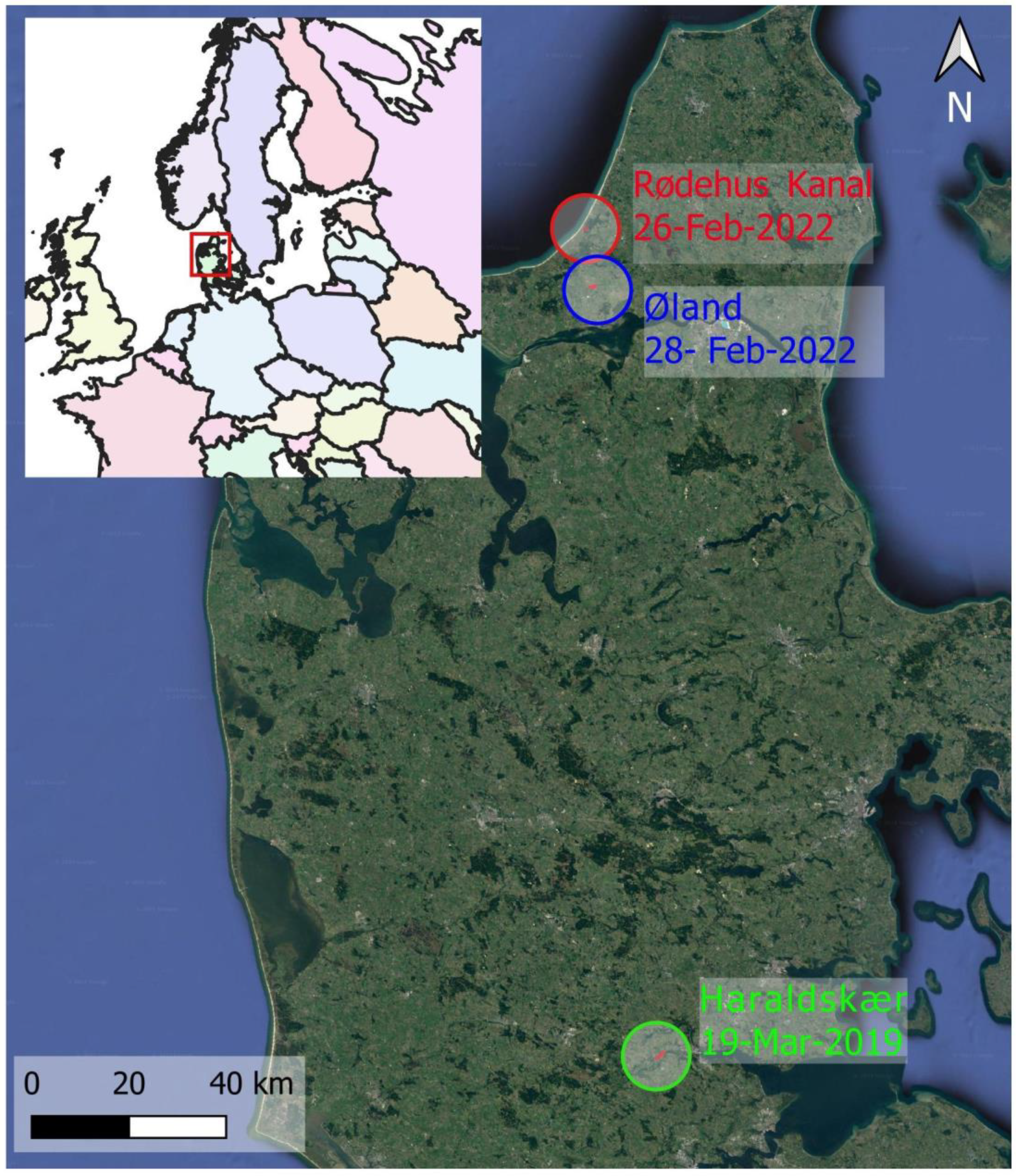
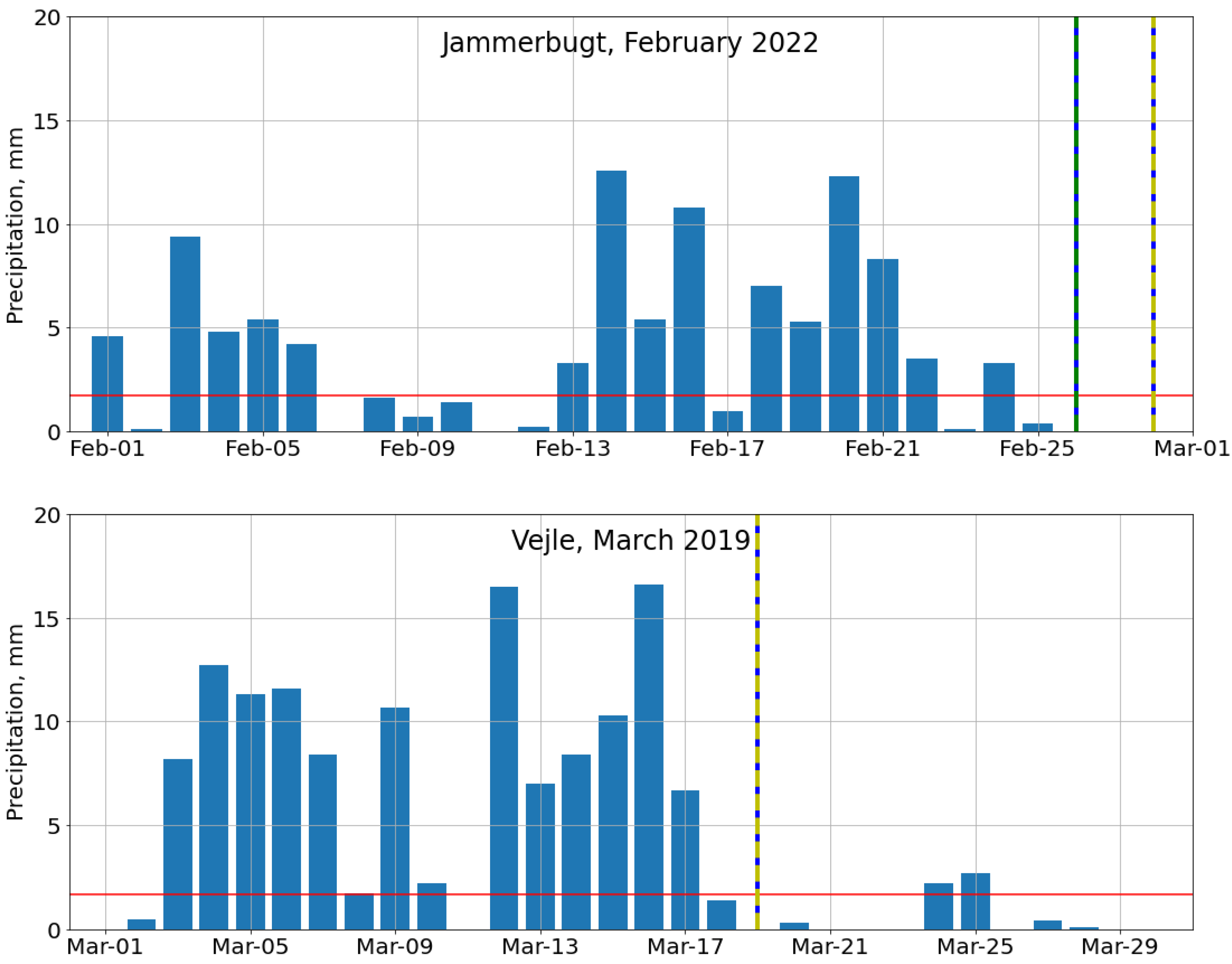
Figure 1 provides and overview of localities mapped with UAS thermal imagery and satellite EO. The Rødehus Kanal and Øland areas are located in the Danish Jammerbugt municipality. The UAS surveys were flown on 26 February and 28 February 2022, respectively. February 2022 was a wet month in Jammerbugt municipality (Figure 2, top panel). The monthly rainfall was 105.8 mm (long-term average for February in Denmark: 48 mm). The cumulative precipitation in the 7 days prior to the UAS thermal surveys was 33.2 mm, and the cumulative precipitation in the 14 days prior to the survey was 73.5 mm.

The Haraldskær area is located in the Danish Vejle municipality. The UAS survey was flown on 19 March 2019. March 2019 was a wet month in Vejle municipality (Figure 2, bottom panel). The monthly rainfall was 139.9 mm (long-term average for March in Denmark: 52 mm). The cumulative precipitation in the 7 days prior to the thermal survey was 66.9 mm, and the cumulative precipitation in the 14 days prior to the survey was 112.8 mm. Flooding was informally observed on the ground in late February 2022 in Jammerbugt municipality and, in March 2019, in Vejle municipality by citizens and local media.

2.2. Surface Water Extent Mapping with UAS Thermal Imagery

RGB and thermal mapping using UAS have become mature surveying techniques providing ground resolution at the cm level and flexible spatial and temporal coverage. Flooding can be delineated from both RGB and thermal imagery. Here, we opted for a thermal mapping workflow because thermal mapping is independent of daylight conditions, which pose severe restrictions on survey schedules in Denmark in winter, and because thermal mapping can reliably detect shallow flooding below low-density vegetation, for instance, in grasslands and agricultural areas.

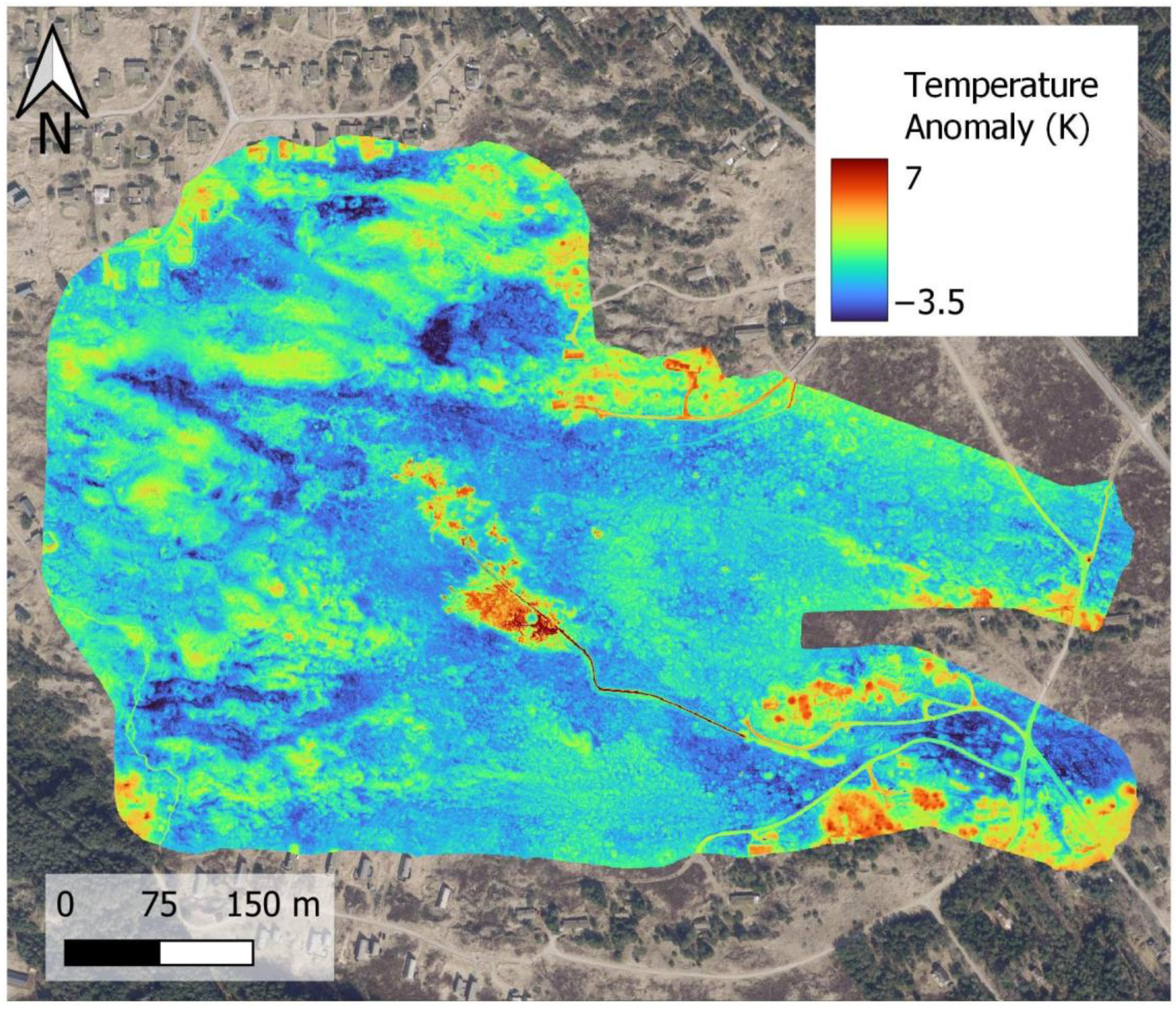
Drone Systems collected thermal imagery using a FLIR Tau-2 thermal camera (Teledyne FLIR, Wilsonville, OR, USA) equipped with a TeAX thermal capture system (TeAX, Wilnsdorf, Germany). Surveys were flown using a Matrice 600 Pro (DJI, Shenzhen, China) platform. Survey flight height was 110–120 m above ground, which resulted in a 15 cm ground resolution of the thermal imagery. Thermal imagery was corrected for drift and sensor non-uniformity artifacts, mosaicked, and subsequently georeferenced using terrain features that could be detected on both the thermal scene and high-resolution airborne imagery. The thermal mapping workflow used here is equivalent to the Drone Systems commercial surveying service [23]. An example of the output of the thermal mapping workflow is provided in Figure 3 for the Rødehus Kanal area.

In Figure 3, warmer areas are detected in flooded areas and open water as well as on buildings and vegetated areas. This is common for flooding events occurring during the cold season. However, it is also evident that warm temperature anomalies occur not only on flooded areas but also on vegetated areas and buildings, i.e., whenever the thermal camera does not record the ground surface temperature, but the temperature of an intermediate surface, such as the top of the canopy or the rooftop of a house. Buildings are typically warmer than the surroundings in the cold season because they are heated. We also observe warmer temperature on canopy surfaces, possibly because of the rainwater storage on the canopy, or due to their higher elevation of canopy surfaces and strong temperature gradients in the atmospheric surface layer.

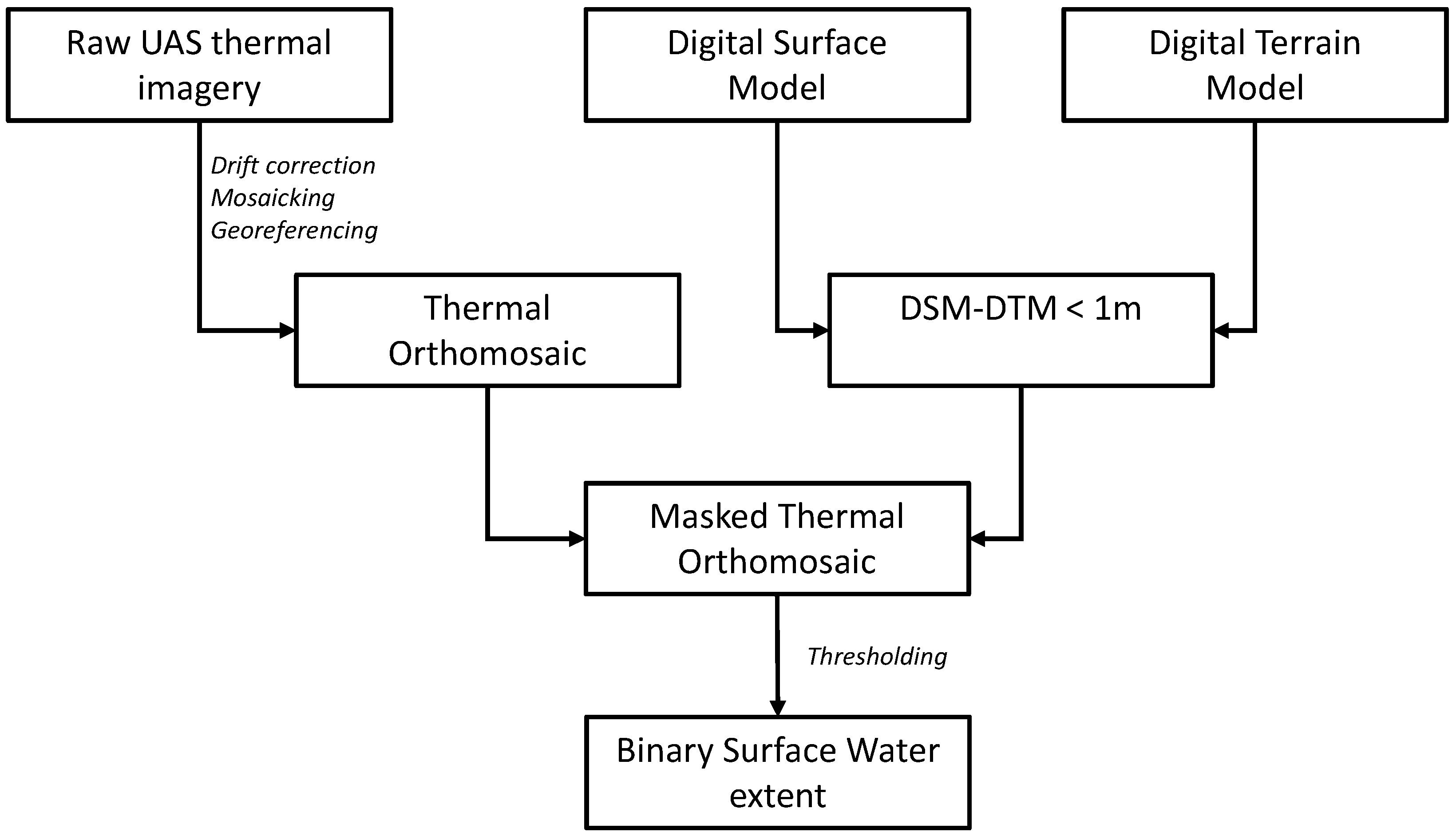
In order to mask buildings and areas covered by vegetation canopy, we used the Danish national elevation model (Danmarks Højdemodel, [24]), which is derived from airborne laser scanning surveys covering the entire country. The raw laser point cloud, consisting of 415 billion individual points, was processed into a digital surface model (DSM) at 0.4 m spatial resolution [25], which is publicly available on the internet. The digital surface model was further processed into a digital terrain model (DTM, [26], also at 0.4 m spatial resolution), by removing buildings, vegetation, etc., from the DSM and interpolating the underlying terrain elevation from neighboring points. We calculated the elevation difference between the DSM and the DTM. Whenever this difference exceeded 1 m, we assumed that the thermal camera did not map ground temperature and, consequently, we masked the corresponding area and excluded it from the surface water extent map, setting the pixel value to undefined (NaN). The flooding status of the masked areas cannot be determined from airborne thermal imagery. We calculated the local sensitivity of the masked area to the 1 m elevation difference threshold and found a limited sensitivity of 26.2 m² of masked area per square kilometer of terrain per m of threshold change for the Rødehus Kanal area (16.3 m²/km²/m for Vejle and 2.5 m²/km²/m for Øland). For this reason, the 1 m threshold in elevation difference can be considered as robust for the areas investigated in this study, and we applied it consistently throughout the analysis. We suggest that the sensitivity of the threshold value is re-checked whenever the UAS thermal SWE mapping workflow is applied to new areas of interest.

Finally, we manually set the threshold for the masked temperature image in order to obtain a binary SWE map. Pixels that are warmer than the threshold are assigned the flooded status (1) and pixels that are cooler than the threshold are assigned a dry status (0). Masked areas and areas not covered by the thermal imagery were assigned undetermined flooding status (NaN). The temperature threshold was set based on the observed temperature of permanent water bodies (streams and lakes) located in the thermal image. Alternatively, automatic thresholding algorithms, e.g., Otsu thresholding, could be used, but because of the low proportion of flooded pixels in the thermal scenes, we do not observe a clear bimodal distribution in the histograms of pixel temperature values. For the areas investigated here, it was straightforward to pick the temperature threshold from observed permanent water bodies located in the thermal scenes. A flowchart of the UAS SWE mapping workflow is presented in Figure 4.

2.3. Surface Water Extent Mapping with Satellite EO

The SWE mapping using satellite EO data was carried out following the methodology reported in [27]. The approach uses a multivariate logistic regression model to estimate surface water probability from a combination of optical imagery from the Sentinel-2 mission and synthetic aperture radar (SAR) imagery from the Sentinel-1 mission. Prior to water classification, all acquired data are subject to essential pre-processing, including standard processing routines for orthorectification, radiometric and atmospheric correction, and cloud masking, as well as terrain and radar shadow masking and noise filtering. For further information about the development of the logistic regression model, the reader is invited to refer to Druce et al. [27]. In the original approach by Druce et al. [27], the input data are processed into monthly composites, but specifically for Danish conditions, we modified the algorithm to output the results by individual sensor and acquisition date without re-training, thereby enabling the SWE products to correspond with the time of the flooding/drone activity. Cloud free, optical data were prioritized due to the ability to identify smaller features than Sentinel-1. This is explained by the characteristics of the input data, with key spectral water detection bands from Sentinel-2 available in 10 m spatial resolution, while the true spatial resolution of Sentinel-1 is understood to be closer to 20 × 20 m, although data from the widely used Sentinel-1 Ground Range Detection (GRD) product are delivered with a pixel spacing of 10 × 10 m [28]. In addition, SAR imagery is typically spatially smoothed to reduce speckle noise; however, this was not undertaken due to the small size of the flood extent. Nevertheless, optical data will often not be available at the time of flooding due to the presence of clouds. After sensor selection, the resulting water probability was inspected, and a user-defined threshold was applied to create the binary surface water extent classification. For the Rødehus Kanal and Øland areas, Sentinel-1 data dated 28-Feb-2022 and Sentinel-2 data dated 26-Feb-2022 were used. For the Haraldskær area, Sentinel-2 data dated 19-Mar-2019 were used. Sentinel-1 data were not available for the Haraldskær area during the period of flooding.

2.4. Validation against the Hydrographically Processed DEM

The Danish national elevation model was further processed by the Danish Agency for Data Supply and Infrastructure into a so-called Bluespot product [29]. Each pixel value of the Bluespot product indicates the amount of rainfall in millimeters that is required to flood that pixel. This value is derived under the assumptions that the terrain surface is impervious (i.e., zero infiltration, no drainage), that the rainfall is uniformly distributed in space, that evapotranspiration is zero, and that water on the land surface moves instantaneously against the terrain elevation gradient and accumulates in local depressions. The Bluespot product thus indicates areas of potential flooding caused by rainfall, and it is therefore useful to compare the product with the SWE maps derived from UAS and satellite EO. However, it is important to note that the Bluespot product outlines areas of potential flooding and that actual flooding is expected to occur only on a subset of Bluespot areas because some of them may be located on soils with high infiltration capacity and/or drained areas. Moreover, riverine flooding (i.e., flooding caused by river water flowing over the riverbanks) will not be confined to Bluespot areas because it is not caused by local rainfall and will not only occur in local depressions. We generally used a threshold of 10 mm to outline potentially flooded areas from the Bluespot product, i.e., areas with a Bluespot value between 0 and 10 mm were mapped as potentially flooded areas.

3. Results

In this section, we present the SWE mapping results for the three survey sites separately.

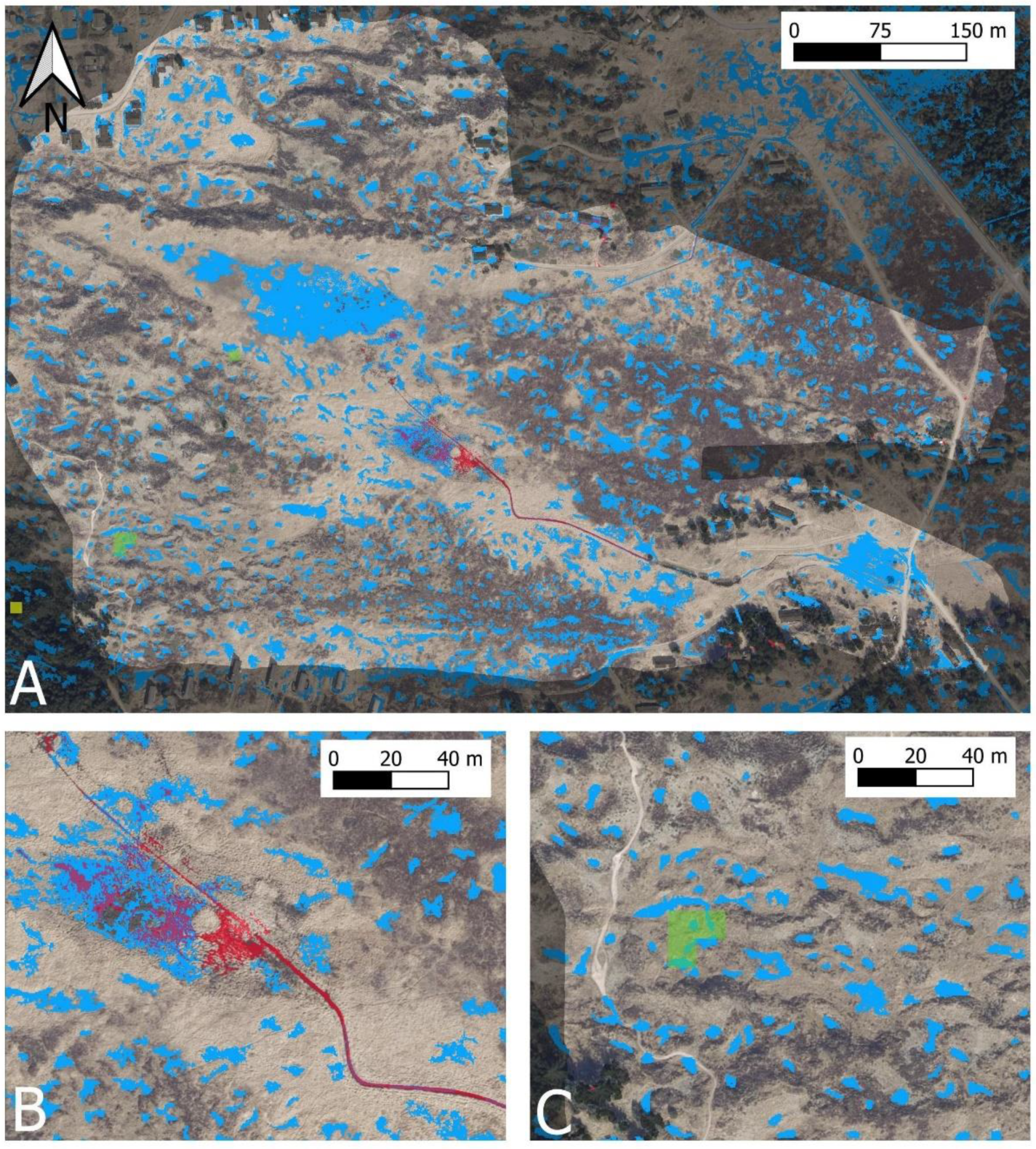
Figure 5 shows UAS and satellite EO SWE mapping results along with Bluespot areas for the Rødehus Kanal site. It is evident that the UAS workflow delineates flooding mainly along a small stream flowing across the site (Figure 5B); 50.1% of the inundated area delineated from thermal imagery does not fall on Bluespot areas (

Table 1. Contingency table for the Rødehus Kanal area. We only report contingency tables for Sentinel-1 SWE because the only pixel mapped as flooded by Sentinel-2 is located outside the thermal scene.

Bluespot vs. UAS SWE (0.4 m pixels)
	Inside Bluespot	Outside Bluespot
UAS flooded	6435	6468
UAS not flooded	281,799	1,917,380
Bluespot vs. Satellite SWE (10 m pixels)
	Inside Bluespot	Outside Bluespot
Sentinel-1 flooded	4	0
Sentinel-1 not flooded	2610	1199
UAS vs. Satellite SWE (10 m pixels)
	Sentinel-1 flooded	Sentinel-1 not flooded
UAS flooded	0	189
UAS not flooded	4	3620

). This is consistent with the riverine origin of the flooding. The satellite SWE mapping workflow classifies just four 10 m pixels falling within the boundaries of the thermal scene as flooded, based on a Sentinel-1 SAR scene recorded on 28-02-2022 (Figure 5A,C). We only report the results for Sentinel-1 SWE because the only pixel mapped as flooded by Sentinel-2 is located outside the thermal scene. In order to compare Bluespot and UAS flood maps with 0.4 m spatial resolution to the satellite SWE mapping results with 10 m resolution, we aggregate the binary Bluespot and UAS flooding maps to 10 m resolution using an “any pixel” rule. This rule implies that the 10 m pixel is assigned a value of 1, if any of the 0.4 m pixels falling on each 10 m pixel have a value of 1; otherwise, the pixel is assigned a value of 0. All pixels classified as flooded based on satellite EO fall on Bluespot areas. However, despite the use of the “any pixel” aggregation rule, which enlarges the area classified as flooded compared to the native 0.4 m resolution, none of the four pixels classified as flooded based on satellite EO fall on pixels that are delineated as flooded by the UAS workflow. The flooded areas delineated using the UAS workflow are hydrologically consistent, occurring mainly adjacent to the stream, which was likely flooded after the substantial rainfall in February 2022. In contrast, the flooded areas delineated by satellite EO appear to be randomly located in the landscape and were not confirmed by informal observations on the ground.

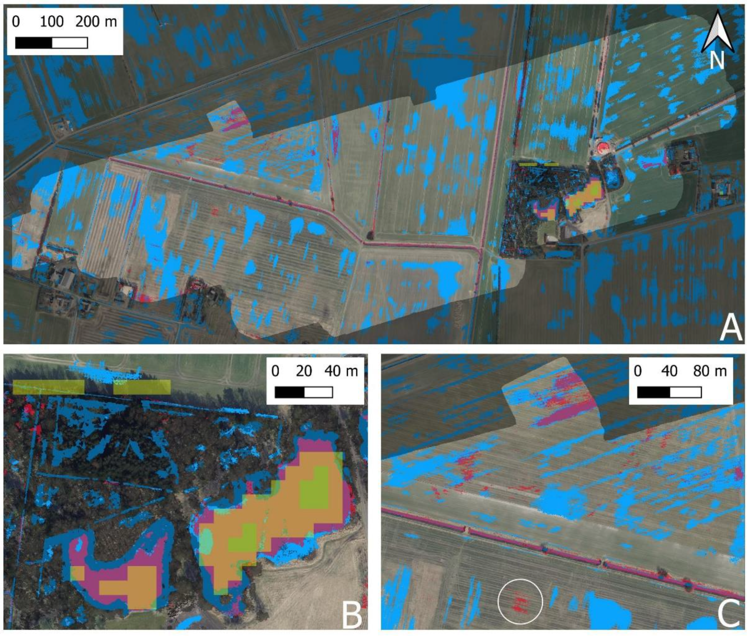
Figure 6 shows UAS and satellite EO SWE mapping results along with Bluespot areas for the Øland site. Unlike the Rødehus Kanal site, the Øland site includes two permanent lakes, which are reliably classified as flooded by both the UAS and the satellite flood mapping workflows (Figure 6B). It is evident from the results that the Sentinel-1 SAR-based mapping delineates a smaller area of the permanent lakes than the mapping based on Sentinel-2 multispectral data and that the Sentinel-2 multispectral results are in better agreement with the UAS results than the Sentinel-1 SAR results. On Figure 6, panel B, Sentinel-2 misclassifies some pixels located in the shaded area of the forest as water. We see similar behavior in the Haraldskær area (see below). While the satellite EO mapping workflow reliably maps the permanent lakes, it does not detect any flooded areas on open fields. In contrast, the UAS mapping workflow identifies at least five hotspot areas of flooding in the open agricultural fields. The majority of the areas mapped as flooded by the UAS workflow fall on Bluespot areas, which supports the validity of the UAS mapping workflow because these floods clearly are of pluvial origin. One sizeable patch of flooded terrain in the UAS results does not fall on a Bluespot area (white circle in Figure 6C). This patch falls on a field on which the ploughing direction has changed between the date when the national elevation dataset was acquired and the date of thermal mapping. It is evident from the Bluespot dataset in this area that the field was ploughed in the north–south direction at the time of laser scanning for the national elevation dataset, while the UAS thermal mapping indicates ploughing in the east–west direction. This shows that in flat terrain, minor changes in elevation can determine the location of pluvial inundation patches.

Table 2. Contingency table for the Øland area.

Bluespot vs. UAS SWE (0.4 m pixels)
	Inside Bluespot	Outside Bluespot
UAS flooded	115,146	61,418
UAS not flooded	969,260	4,656,767
Bluespot vs. Satellite SWE (10 m pixels)
	Inside Bluespot	Outside Bluespot
Sentinel-1 flooded	8	0
Sentinel-1 not flooded	5306	4729
Bluespot vs. Satellite SWE (10 m pixels)
	Inside Bluespot	Outside Bluespot
Sentinel-2 flooded	63	3
Sentinel-2 not flooded	5251	4726
UAS vs. Satellite SWE (10 m pixels)
	Sentinel-1 flooded	Sentinel-1 not flooded
UAS flooded	8	2406
UAS not flooded	0	7629
UAS vs. Satellite SWE (10 m pixels)
	Sentinel-2 flooded	Sentinel-2 not flooded
UAS flooded	59	2355
UAS not flooded	7	7622

provides contingency tables for the comparisons between UAS, satellite, and Bluespot datasets. Bluespot and UAS results were upscaled to 10 m using an “any pixel” rule as described for the Rødehus Kanal area.

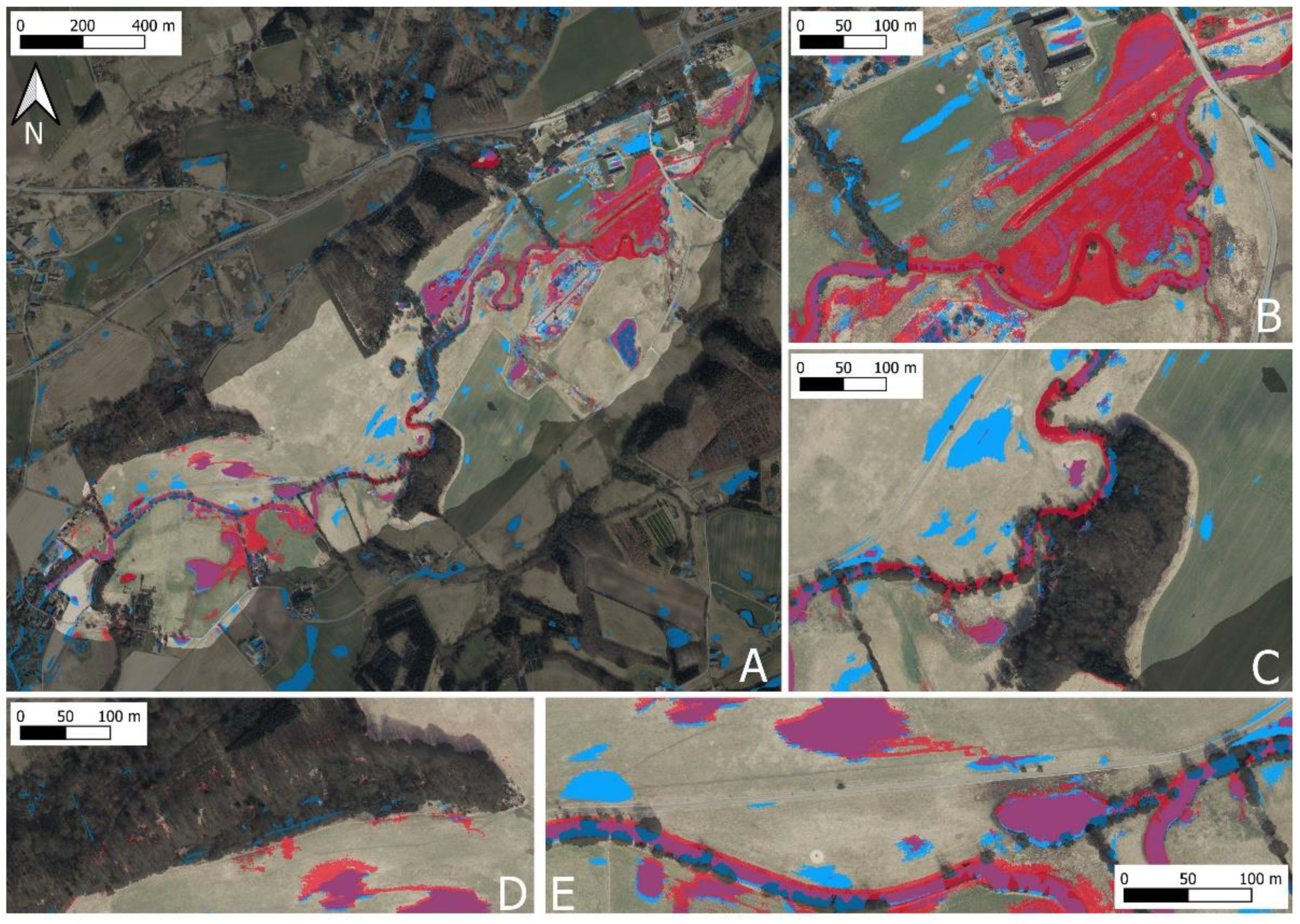
Figure 7 shows UAS and satellite EO SWE mapping results along with Bluespot areas for the Haraldskær site. Haraldskær is the largest of the three sites, and both the satellite EO and the UAS mapping workflows delineate sizeable areas of both pluvial and riverine flooding (

Table 3. Contingency table for the Haraldskær area. We only report contingency tables for Sentinel-2 SWE because no Sentinel-1 results are available for the date of the UAS thermal survey.

Bluespot vs. UAS SWE (0.4 m pixels)
	Inside Bluespot	Outside Bluespot
UAS flooded	547,657	672,873
UAS not flooded	351,367	7,908,880
Bluespot vs. Satellite SWE (10 m pixels)
	Inside Bluespot	Outside Bluespot
Sentinel-2 flooded	1426	1168
Sentinel-2 not flooded	2471	13,049
UAS vs. Satellite SWE (10 m pixels)
	Sentinel-2 flooded	Sentinel-2 not flooded
UAS flooded	1984	3470
UAS not flooded	610	12,050

). We only report results for Sentinel-2 SWE because no Sentinel-1 results are available for the date of the UAS thermal survey. In general, there is good agreement between the flooded areas outlined by the satellite EO and the UAS workflow. Flooded areas caused by riverine flooding outlined by the UAS workflow tend to be slightly larger (Figure 7B) as the ones outlined by satellite EO. Similar behavior was observed on the permanent lakes in the Øland area. Just as in the Øland area, Sentinel-2 risks misclassifying pixels as flooded that are located in forested or shaded areas (Figure 7C,D). It is evident from Figure 7E, that flooded areas tend to locate on Bluespot areas. However, only a fraction of Bluespot areas become flooded, while others remain dry.

Table 3 reports the contingency tables for the comparisons between UAS, satellite EO, and Bluespot areas. The majority of areas classified as flooded by both the UAS and satellite EO workflow are located inside Bluespot areas. However, a sizeable fraction of the flooded pixels falls outside the Bluespot areas, which is consistent with the riverine flooding occurring in the downstream portion of the Haraldskær area (Figure 7B). Table 3 shows that the flooded area mapped by UAS is significantly larger than the area mapped as flooded from Sentinel-2. One reason is the “any pixel” rule used to resample the UAS flooding maps from 40 cm resolution to 10 m resolution. Another reason is the Sentinel-2 under-estimation of the flooded areas along the fringes of water bodies, which was observed both in the Øland and Haraldskær areas.

4. Discussion

Predicting flood risk and forecasting actual flooding become ever more important with increasing frequency, severity, and impact of flood events. At the same time, mapping surface water extent remains challenging, particularly for low-gradient environments with complex hydrography and small-scale flooding patterns. Flood modelers thus often face the problem that the true surface water extent is unknown and cannot be systematically mapped at the appropriate scale and spatial resolution. This paper presents a UAS thermal mapping workflow that can deliver surface water extent maps at a native spatial resolution better than 10 cm, depending on the flight height. Based on comparisons with the Bluespot product derived from the national elevation model of Denmark and on independent informal flood observations in the study areas (i.e., ground-based photography at flooded locations), which were not used in the generation of any of the flood mapping results, we are confident that the UAS mapping workflow delivers SWE maps that are close to the actual inundation patterns on the ground, for areas without dense vegetation cover. However, it is important to note that the results of the UAS thermal SWE mapping workflow were not systematically compared to SWE ground truth in this paper because such ground truth observations are unavailable at the scale covered by the UAS thermal surveys.

Despite the high fidelity of flood maps delivered by the UAS mapping workflow, the workflow is not suitable for operational flood monitoring and surveillance at high temporal resolution and wide spatial coverage. Using multirotor platforms, UAS mapping workflows can cover areas of about a few square kilometers per day. Spatial coverage can be significantly increased using fixed-wing platforms, but regional-scale operational monitoring remains impractical. Thus, satellite EO and/or models will remain the methods of choice for operational flood monitoring at the regional scale. However, models and workflows based on satellite EO need to be validated and benchmarked against high-fidelity datasets in order to assess and document their skill. UAS flood maps can play a key role in this context because they provide reliable inundation maps at very high spatial resolution. Our study showed that a flood mapping workflow based on public data from the Sentinel missions reliably maps permanent water bodies in the chosen test regions, while small-scale flooding caused by excess rainfall on grasslands and agricultural fields was not identified with confidence. Sentinel-2 flood maps show a higher number of true positives when compared to UAS flood maps than Sentinel-1 flood maps. However, unlike Sentinel-1 SAR, Sentinel-2 spectral mapping is not possible under cloud cover, which severely restricts the temporal resolution of flood maps. Overall, it seems that UAS mapping reliably detects flooding in the right places, while the spatial resolution of Sentinel datasets seems to be insufficient to detect small-scale flooding. Higher spatial resolution commercial alternatives to the Sentinel missions exist (e.g., TerraSAR-X, [30]) but come at a higher cost. Depending on the specific application of the mapping workflow, an appropriate data value analysis should therefore be carried out to ensure that additional costs are justified in terms of the enhanced prediction skill. Such evaluations must be based on the comparison of predicted flood maps with “ground truth” for selected events in the historical record. UAS mapping workflows can play a key role in this context as they can provide high-fidelity, high-resolution flood maps for selected areas and events. An important consideration for choosing the SWE mapping method is cost: many satellite EO missions provide free and open data, but data processing workflows require computational infrastructure and expertise. UAS mapping workflows require significant data processing resources and, additionally, resources for field surveys (UAV platform, sensor payloads, operators, and logistics).

5. Conclusions

We conclude that UAS thermal mapping is an efficient surveying technique that delivers SWE maps with high fidelity and high spatial resolution for intermediate scales ranging up to a few square kilometers. Such high-fidelity flooding maps are useful to calibrate, benchmark, and validate models and flood mapping algorithms based on satellite earth observation.