
Daily Rhythms and Oxygen Balance in the Hypersaline Lake Moynaki (Crimea)
by
 , , ,
, , ,
Nickolai Shadrin
1,
Elena Anufriieva
1,*,
Alexander Latushkin
1,2,
Alexander Prazukin
1 and
Vladimir Yakovenko
1 1
A.O. Kovalevsky Institute of Biology of the Southern Seas of RAS, 2 Nakhimov Ave., 299011 Sevastopol, Russia
2
Marine Hydrophysical Institute, Russian Academy of Sciences, 2 Kapitanskaya St., 299011 Sevastopol, Russia
*
Author to whom correspondence should be addressed.
Water 2022, 14(22), 3753; https://doi.org/10.3390/w14223753
Submission received: 24 September 2022
/
Revised: 15 November 2022
/
Accepted: 17 November 2022
/
Published: 18 November 2022
(This article belongs to the Special Issue Ecosystems of Inland Saline Waters)
Abstract
:Field observations of the diurnal behavior of several parameters (oxygen concentration, chlorophyll fluorescence, photosynthetically active radiation (PAR), wind speed, temperature, suspended matter concentration, and zooplankton abundance) were conducted at three sites in the marine hypersaline lake Moynaki (Crimea). The diurnal course of PAR followed a bell-shaped form, with the maximum at 14:00 on the 15th and 16th of September 2021. The oxygen concentration varied over a wide range from 3.2 to 9.3 mg L−1, demonstrating a clear diurnal rhythm. From sunrise until about 17:30, it increased. Both the maximum and minimum values were marked on the site where there were Ruppia thickets. The daily rhythm of Chlorophyll a concentration was clearly expressed during the observation period, varying from 2.49 to 18.65 µg L−1. A gradual increase in the concentration of chlorophyll a began after 10:00 and lasted until about 2:30–3:00 of the next day. The daily production of oxygen during photosynthesis averaged 27.3 mgO L−1 day−1, and the highest values were noted at the windward site of 37.9 mgO L−1 day−1, and the lowest at the leeward site of 19 mgO L−1 day−1. The total respiration of the community per day was, on average, 15.9 mgO L−1 day−1. It averaged 63% of the primary production created. The contribution of animals to the total oxygen consumption of the community was small, averaging 5%.
1. Introduction
The rotation of the Earth around its axis creates the daily solar radiation rhythms driving the variability of energy supply to all ecosystems, including aquatic ones. The formation of primary productivity is carried out mainly by photosynthesis, which in turn depends on the incoming PAR (the photosynthetically active part of the sunlight flux) as well as on nutrient availability and, of course, temperature. The rhythms of all processes in ecosystems, therefore, must somehow adapt to the rhythms of primary production, set by PAR. Based on this, it would be logical to assume that all rhythms are expressed similarly in water bodies of every climate zone. However, ecosystems are complex systems with many non-linear intertwining relationships and are capable of being in alternative states [1,2,3,4]. Thus, it is difficult to unambiguously describe the impact of PAR influx rhythm on the components and processes of ecosystems [5,6,7,8].
The concentration of dissolved oxygen in a water body is determined primarily by gross primary production (oxygenic photosynthesis), ecosystem respiration, and exchange with the atmosphere [9,10,11]. The diurnal fluctuations in dissolved oxygen content, therefore, make it possible to evaluate whole ecosystem metabolism, which outlines carbon (C) accumulation and breakdown in ecosystems [12,13,14]. Dissolved oxygen concentration can therefore serve as a good integral indicator of diurnal changes in ecosystem functioning. Currently, more studies are demonstrating that diurnal rhythms of changes in oxygen concentration have their characteristics in different aquatic ecosystems [8,15,16,17,18,19]. Unfortunately, among these studies, the relationship between the daily rhythms of various parameters in ecosystems of hypersaline waters has not been analyzed. At the same time, it has been shown that high salinity can accelerate the exchange of gases between a water body and the atmosphere by several times [20,21]. Thus, saline and hypersaline lakes play a significant role in global gas exchange between water bodies and the atmosphere; in addition, some of them can provide a high rate of C burial, up to 60% of total primary production [22,23,24] Thus, the study of such lakes is relevant because it is assumed that they may act as an effective natural mechanism for slowing down global warming [23,24].
The more complex an ecosystem, the more species it contains, and the more difficult it is to understand the variety of causes and relationships and to understand how the rhythms of some components affect the rhythms of others. Ecosystems of hypersaline waters, existing in a polyextreme environment, are characterized by reduced biodiversity [25,26], therefore, it can be assumed that, when studying them, it will be easier to understand the interweaving of causes and effects. At the same time, it is necessary to note one of the important features of such ecosystems. With an increase in salinity, the solubility of oxygen in water decreases sharply [27,28,29]. For example, for 25 °C, the dependence can be described by the equation [30]:
where DOsat—oxygen solubility, mg L−1; S—salinity, g L−1.
DOsat = 8.268e−0.006S,
According to Equation (1), the solubility of oxygen at a salinity of 40 g L−1 will be 6.5 mg L−1 and at a salinity of 200 g L−1 is 2.5 mg L−1. Due to this, the oxygen regime in hypersaline water bodies has its specifics, but there are practically no data on the nature of daily changes in oxygen concentration in a hypersaline environment. Other studies are demonstrating that oxygen concentration in hypersaline environments can vary from 0 to 200% saturation during the day [25]. Small hypersaline lakes with underwater vegetation and low biodiversity often demonstrate extreme environmental variability with intensive photosynthesis and carbon cycling [14,25]. These small lakes can be used as natural field laboratories to study the integration of different parameters and processes within a daily rhythm. There are many hypersaline lakes in Crimea [25,31]; daily changes in oxygen concentration and several other parameters were studied in one of them. In this study, the authors also took into account the variability of the wind, as wind affects the exchange of the lake with the atmosphere [11,27,32] and other processes.
The aim of the study was as follows: 1. to conduct field observations of the diurnal behavior of several parameters (oxygen concentration, chlorophyll a fluorescence, illumination, wind speed, temperature, suspended matter concentration, and zooplankton abundance); 2. to assess the nature of the relationship between the studied characteristics; 3. to assess the possible role of animals in diurnal changes in oxygen concentration. 4. to confirm or refute the assumptions that (a) the wind affects the spatial distribution of many ecosystem parameters, (b) in macrophyte thickets, the range of daily fluctuations in oxygen concentration is higher than in areas where they are absent, or (c) hypersaline lakes may supply more oxygen to the atmosphere than they absorb.
2. Materials and Methods
2.1. Study Area
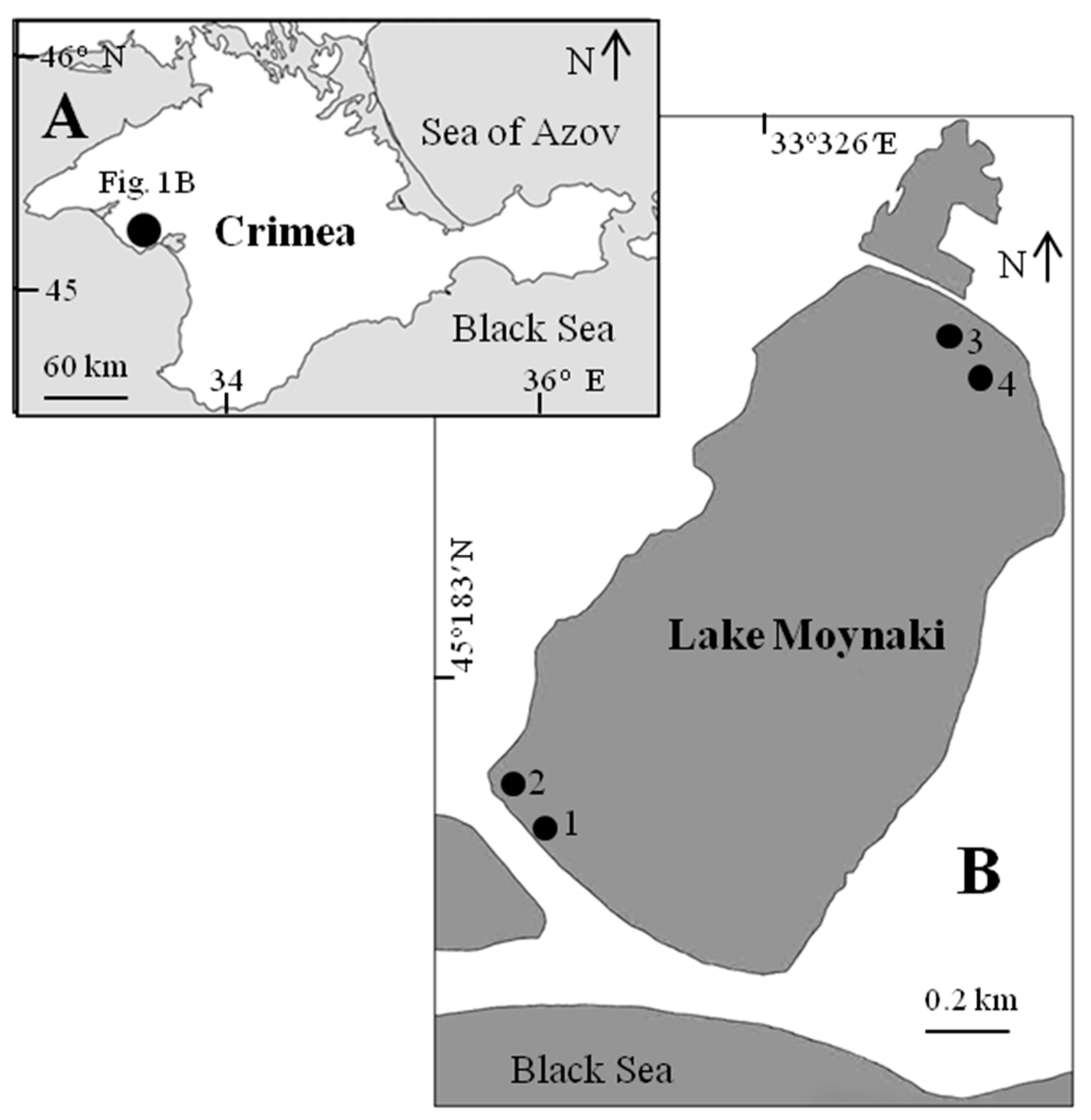
The marine hypersaline lake Moynaki (45°10′37″ N, 33°18′50″ E) is situated in West Crimea (city of Yevpatoriya) and is separated from the Black Sea by a sand spit with an average width of 300 m (Figure 1). It has been used as a model lake for several different studies [33,34,35]. It has a length of about 1.85 km, an area of 1.76 km2, and a depth from 0.45 to 1.00 m. The lake salinity varied between 160 and 200 g L−1 before the 1970s, and after that, due to the increased agricultural and municipal freshwater discharge, it started gradually decreasing: 80 g L−1 in 1986 and 60–70 g L−1 in 1996, and, in 2000–2021, it fluctuated between 45 and 65 g L−1. The faunistic and floristic composition was dramatically changed due to this. Currently, there are patches of the marine grass Ruppia maritima Linnaeus, 1753. Animal species richness is low, the most common being three species of Cladocera (Moina salina Daday, 1888 dominates), two or three species of Harpacticoida, one Ostracoda species (Eucypris mareotica (Fischer, 1855), one Amphipoda (Gammarus aequicauda (Martynov, 1931)), and one Chironomidae (Baeotendipes noctivagus (Kieffer, 1911)). Phytoplankton blooms often occur in the lake.
2.2. Methods
Studies of the daily changes of all parameters excluding zooplankton and benthos were carried out on the 15th and 16th of September 2021 at three Lake Moynaki sites, 13 times in total. Between measurements and sampling in the different sites, there were no more than 40 min. A zooplankton and benthos study had been carried out at the same sites some days prior, 6 times. The measurements of temperature, salinity, oxygen, chlorophyll a content, and total suspended solids (TSS) were made by an Aqua TROLL 500 Multiparameter Sonde (In-Situ Inc., Fort Collins, CO, USA). Each time, for three minutes, 280–320 evaluations of every parameter were done. Measurements of photosynthetically active radiation (PAR) were carried out in the daytime at a depth of 10 cm using an underwater quantum sensor Li-192SA (Li-COR, Lincoln, NE, USA). Wind direction and speed were measured at a height of 3 m by an anemometer Megeon 11030 (Megeon, Moscow, Russia). For zooplankton sampling, water (100 L) was filtered through a plankton net with a mesh size of 110 μm, and benthic samples were taken by a benthic tube (diameter 5 cm) as before [33,34,35]. All samples were processed under a stereomicroscope Olympus SZ61TR (Olympus, Tokyo, Japan) using a Bogorov chamber with species identification and size measuring.
2.3. Data Processing
All obtained data were subjected to standard statistical processing. The mean values, coefficients of variation (CV), correlation (R), and determination (R2), as well as the parameters of the regression equations, were calculated in the standard MS Excel 2007 program. For correlation coefficients, the confidence level (p) was determined [36]. An evaluation of the significance of differences in average values was done using normality tests [37] and then a Student’s t-test.
The determination of parameters of oxygen balance in the lake was done using obtained data and known relations. The balance of oxygen in the water column was determined as follows [9,11]:
where ΔDO/Δt is the change in the dissolved oxygen concentration during time interval Δt; GPP is gross primary production; R is ecosystem respiration; F is the exchange of O2 between the water surface and the atmosphere; A is a term that combines all other processes that cause changes in dissolved oxygen concentration at the sampling site.
ΔDO/Δt = GPP − R − F − A,
In further calculations, we assume that the sum of all unaccounted-for processes (A) can be equated to zero. The rate of exchange with the atmosphere is usually described by the equation [11,32,38]:
where F is the exchange of O2 between the water surface and the atmosphere, mg O2 m−2 h−1; k is the piston velocity coefficient, m h−1; DOt is the measured O2 concentration, mg L−1; DOsat is the oxygen saturation, mg L−1; Zmix is the depth of the mixing water column, m (the water depth was 0.4 m at the study sites; the water column was mixed, and no vertical temperature change was observed).
F = k (DOt − DOsat)/Zmix,
The oxygen-saturating concentration was calculated according to the instrument data, and Equation (1) differed little in our case, averaging 6.7 O2 mg L−1, CV = 0.096, when the average daily temperature was 20.8 °C (CV = 0.093) and the salinity was 50.2 g L−1 (CV = 0.013). This value was used in further calculations.
At the same time, the coefficient k positively depends on the wind speed [11,32], and its dependence on the wind speed at a height of 3 m above the lake where measurements were taken can be described by the equation:
where W is wind speed, m s−1.
k = (0.215(1.11W)1.7 + 2.07)/100,
The coefficient k negatively depended on temperature; to take this into account, it was multiplied by the coefficient calculated for our case using the well-known formula [11]: at 17 °C it was 0.761, at 18 °C—0.724, at 20 °C—0.622, at 22 °C—0.633, at 24 °C—0.539.
The calculation according to Equation (4), taking into account these temperature corrections, showed that, in the range of observed temperatures from 18 to 24 °C, k variability depends on the wind speed by 99%, and this dependence can be approximated by the equation (R = 0.996, p = 0.0001):
k = 0.012e0.22W,
In further calculations, this equation was used according to Equation (3). Changes in oxygen content (ΔDO/Δt) were determined as follows:
where DO1 and DO2 are the oxygen concentrations (mg O2 m−2 h−1), observed at times t1 and t2 (h), respectively.
ΔDO/Δt = (DO2 − DO1)/(t2 − t1),
ΔDO/Δt calculated for the dark period is the visible dark respiration of the community (excluding exchange with the atmosphere), and calculated for the light period is the visible net oxygen production in the community due to oxygenic photosynthesis, excluding exchange with the atmosphere and light respiration.
The real total dark respiration (RN) was calculated using the equation:
where RN—total dark respiration, mg O2 m−2 h−1, (ΔDO/Δt)N—change in O2 concentration at night, mg O2 m−2 h−1.
RN = (ΔDO/Δt)N + F,
How to calculate all values, except for light (RL) or day respiration (RD), is discussed above, but there is no single approach for estimating RD. It has only been shown that light respiration is higher than the dark respiration of phototrophs and their associated heterotrophs by an average of 20–45% [13,17,39]. Herein, the authors used 35%. At night, the average temperature is lower than during the day; therefore, to reduce daytime respiration, a temperature correction was used, which was calculated through Q10 = 2.25 [40,41,42]:
where R1 and R2 are the oxygen consumption rates, mg O2 h−1 at temperatures T1 and T2 (°C), respectively.
R2 = R1 2.25(T2−T1)/10,
Based on this, the light oxygen consumption was calculated by the formula:
RL = 1.35 RN 2.25(T2−T1)/10,
The total respiration of animals was calculated for the common species and size groups of animals according to the known equations of the dependence of the intensity of oxygen consumption on body weight [43,44,45] and then summed all these values. The calculation gave consumption values at 20 °C, and they were recalculated to the observed temperature according to Equation (8).
3. Results
During the study period, at site 1, the salinity varied from 49.3 to 52.4 g L−1 (average 50.2 g L−1, CV = 0.015), at site 2 from 49.6 to 50.6 g L−1 (average 50.1 g L−1, CV = 0.008), and at site 3 from 48.6 to 51.8 g L−1 (average 50.2 g L−1, CV = 0.013). There were no significant differences in salinity at different stations.
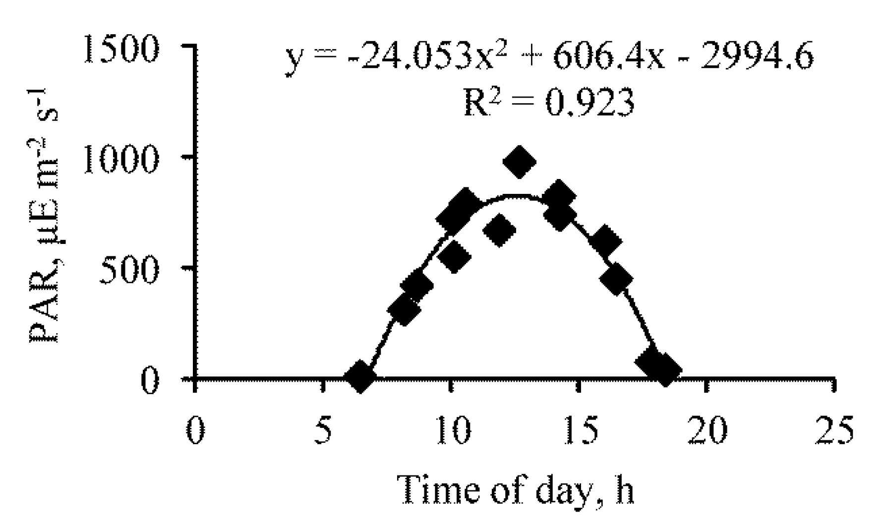
The diurnal course of PAR in the water followed a bell-shaped form, and its maximum was observed during the day, up to 14:00 (Figure 2).
The ascending axis of the bell, from 6:00 to about 13:00, can be described by the equation (R = 0.911, p = 0.001):
where P—PAR (the photosynthetic active part of the sunlight flux), μE m−2 s−1; t—time of day, h.
P = 113.5 t + 45.4,
The descending axis of the bell, occurring after 14:00, can be described (R = 0.975, p = 0.0001):
P = 3276 − 173.8 t,
There was a consistent NE wind during the observation period, so sites 1 and 2 were at the leeward coast, and site 3 was at the windward one. The average wind velocity over the observation period was 4.5 m s−1 (CV = 0.514). At the same time, the velocity significantly (p = 0.01) decreased from 9.0 to 1.8 m s−1 in the period from 10:00 to 20:40 (15 September 2021), and the dependence can be described by the equation (R = 0.698, p = 0.02):
W = 23.4 − 6.4 Ln (t),
In the subsequent observation period, the wind velocity did not change significantly, averaging 2.9 m s−1 (CV = 0.353). During the study period, at site 1, the temperature varied from 17.8 to 23.8 °C (average 20.5 °C, CV = 0.095), at site 2 from 17.9 to 23.9 °C (average 20.5 °C, CV = 0.095), and at site 3 from 18.7 to 24.2 °C (average 21.2 °C, CV = 0.090). There were no significant differences in temperature at different stations. The average water temperature during the observation period ranged from 17.7 to 25.0 °C and was significantly positively correlated with the level of PAR (R = 0.587; p = 0.05) and wind speed (R = 0.707; p = 0.0005). The average salinity in the lake during the observation period was 50.3 g L−1 (the range of fluctuations was from 48.6 to 54.8 g L−1, CV = 0.028). At sites 1 and 3, the temporal variability (CV = 0.046 and CV = 0.014) was higher than at site 2 (CV = 0.008). The spatial variability (between stations) (mean CV = 0.013) was lower than temporal (CV = 0.023).
The oxygen concentration varied over a wide range from 3.2 to 9.3 mg L−1, and both the maximum and minimum values are marked at site 2, where there were Ruppia thickets. No relationship between oxygen concentration and salinity was found. There was a significant positive relationship between oxygen concentration and temperature (R = 0.826, p = 0.005):
where T—temperature, °C.
DOt = 0.66 T − 7.41,
The oxygen content demonstrated a clear diurnal rhythm. From sunrise until about 17:30, the oxygen concentration increased. The average increase in oxygen in this period at site 1 was 0.53 mg L−1 h−1 (CV = 0.204), at site 2 was 1.22 mg L−1 h−1 (CV = 0.367), and at site 3–0.34 mg L−1 h−1 (CV = 0.338). Differences between all three stations are significant (p > 0.01).
For an example, this increase can be described for site 1 by the equation (R = 0.728, p = 0.005):
DOt = 1.83 t0.556,
After 17:00 and until about 6:00 the next day, the oxygen concentration decreased, as an example for site 1 (R = 0.945, p = 0.0001):
where X is the number of hours since the beginning of the countdown, (1 = 5 p.m.).
DOt = 9.31 e−0.063X,
The degree of water saturation correlated with the oxygen concentration (R = 0.986, p = 0.0001):
a = DOsat = 16.54 DOt − 9.65,
Oxygen saturation above 100% was observed at site 1 from 12:00 to 20:30 (maximum 145% at 16:30), at site 2 in the same period (maximum 147% at 14:20), and at site 3 from 12:00 to 20:20 (maximum 119% at 14:20). An oxygen content change had some different relationships with PAR at the three sites. The oxygen content change at site 1 was negative up to PAR of about 80 μE m−2 s−1 and directly correlated with PAR above up to its values of 800 μE m−2 s−1, which can be described (R = 0.967, p = 0.005):
ΔDO/Δt = 0.296 + 0.0005P,
With an increase in PAR above 800 μE m−2 s−1, a slowdown in the growth of oxygen concentration was observed at sites 1 and 2. At site 2, an inverse relationship was observed in the range of PAR from 9 μE m−2 s−1 to 800 μE m−2 s−1 (R = −0.996, p = 0.005):
ΔDO/Δt = 1.34 − 0.0006P,
At site 3, the dependence in the range from 9 to 800 μE m−2 s−1 had a bell-shaped form with a maximum at the illumination of 500–600 μE m−2 s−1 (R = −0.857, p = 0.05):
ΔDO/Δt = 0.002P + 0.244 − 2 × 10⁻⁶ P2,
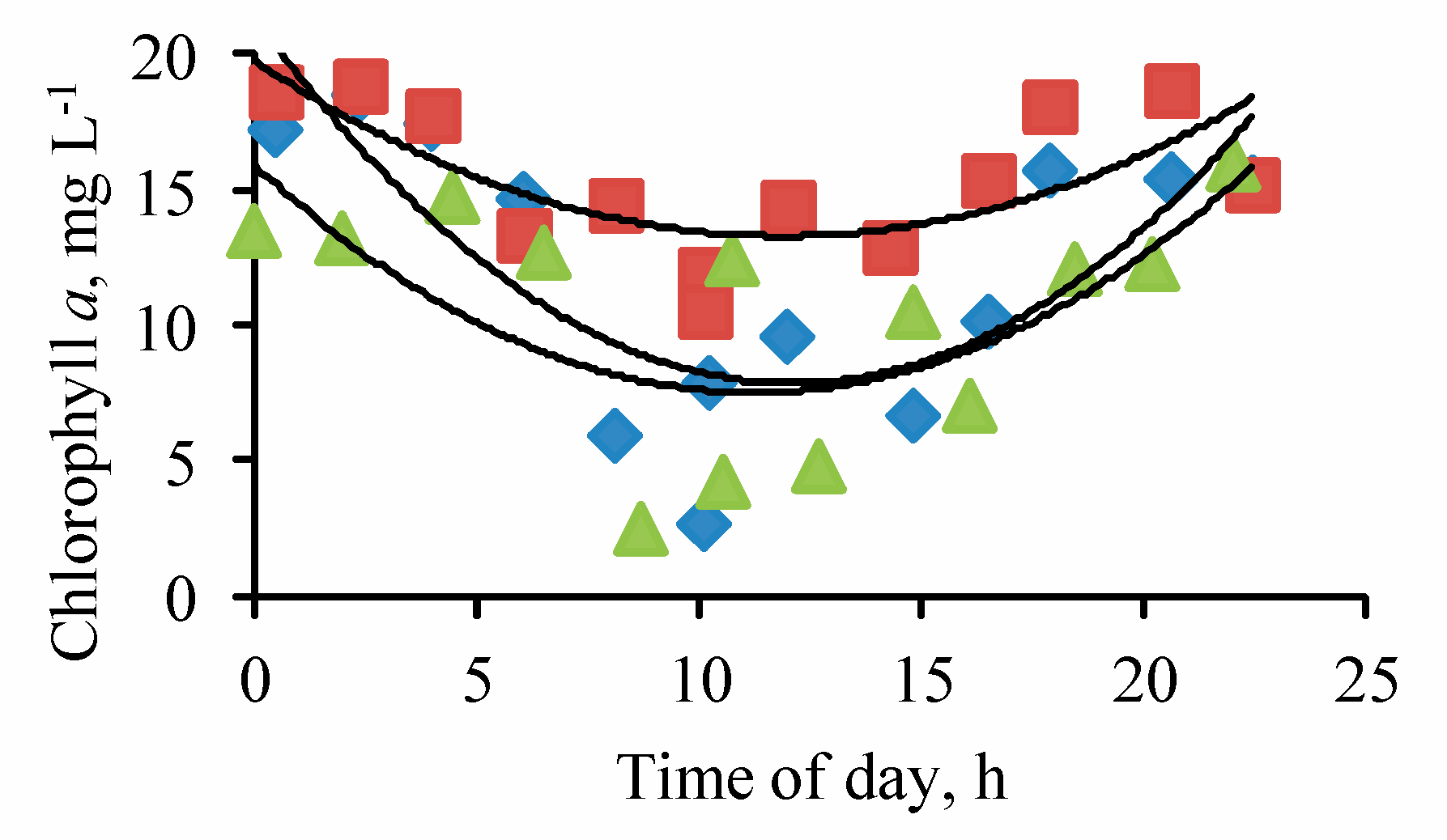
The chlorophyll a concentration during the observation period varied from 2.49 to 18.65 µg L−1, averaging 12.70 µg L−1 (CV = 0.364). The mean concentration over the observation period at site 1 was 12.08 µg L−1 (CV = 0.428), at site 2–15.36 µg L−1 (CV = 0.188), and at site 3–10.64 µg L−1 (CV = 0.422). In its changes, the daily rhythm was clearly expressed, the nature of which changed somewhat from site to site (Figure 3).
At site 1, minimum concentration was observed at about 10:00, 2.65 µg L−1, at site 2—at 10 a.m., 10.50 µg L−1, and at site 3—at 8:40 a.m., 2.49 µg L−1. The maximum concentration of chlorophyll a at site 1 was 18.50 µg L−1 at about 2:30, at site 2 it was 18.81 µg L−1 at 2:38, and at site 3 it was 15.95 µg L−1 at 22:00. A gradual increase in the concentration of chlorophyll a began after 10:00 at site 1 and site 2 and lasted until about 2:30–3:00 the next day, and at site 3, an increase in the concentration of chlorophyll a was observed from 8:45 to about 22:00.
This increase may be described for site 1 (R = 0.950, p = 0.005), site 2 (R = 0.809, p = 0.005), and site 3 (R = 0.867, p = 0.01) by the equations, respectively:
where Ch—the chlorophyll a concentration, µg L−1, and X1—the number of hours from the beginning of the content rise (1 = 10:00 for sites 1 and 2, and site 3, 1 = 8:30).
Ch = 6.95 X110.385,
Ch =13.27 X110.132,
Ch = 5.06 X110.401,
The decrease in the concentration of chlorophyll a after reaching the maximum may be described for site 1 (R = −0.973, p = 0.01), site 2 (R = −0.923, p = 0.02), and site 3 (R = −0.772, p = 0.02) by the equation, respectively:
where X2 is the number of hours from the beginning of the fall in concentration.
Ch = 22.70 − 2.49 X2,
Ch = 19.83 − 1.12 X2,
Ch = 17.77 − 1.14 X2,
At all sites, a significant negative correlation was observed between the concentrations of chlorophyll a and PAR; for sites 1, 2, and 3, respectively, it was described (R = −0.904, p = 0.0001), (R = −0.756, p = 0.001), and (R = −0.642, p = 0.005):
Ch = 16.30 − 0.013 P,
Ch = 17.27 − 0.006 P,
Ch = 13.24 − 0.008 P,
Chlorophyll a concentration and oxygen concentration did not correlate. The increase in the oxygen content during the daytime, as well as its decrease in the dark, did not correlate with the oxygen concentration.
The concentration of total suspended solids (TSS) varied over a wide range from 22.04 mg L−1 to 77.65 mg L−1, averaging 35.13 mg L−1 (CV = 0.326). The average concentration at sites 1 and 2 near the windward coast did not differ significantly, averaging 38.40 mg L−1 (CV = 0.353) and 39.47 mg L−1 (CV = 0.271), but at the third site, it was significantly (p = 0.005) lower than at the other two, on average 27.53 mg L−1 (CV = 0.173). At the first and second sites, there was a significant positive relationship between particle concentration and wind speed, and it may be approximated for site 1 (R = 0.717, p = 0.001) and site 2 (R = 0.568, p = 0.01), respectively:
where TSS—total suspended solids, mg L−1.
TSS = 26.29e0.084W,
TSS = 30.29e0.059W,
This dependence was less pronounced at site 2 with Ruppia vegetation. There was no such dependence at all at site 3 near the leeward coast.
The content of chlorophyll a in suspended matter differed little between the sites, on average 0.34 µg g−1 (CV = 0.499), 0.41 µg g−1 (CV = 0.302), and 0.38 µg g−1 (CV = 0.405) at sites 1, 2, and 3, respectively. During the day, this indicator changed in a similar way as changes in chlorophyll a concentration.
At sites 1 and 2 (near the leeward coast), the wind speed significantly negatively affected the content of chlorophyll a in TSS, which can be described, respectively, as (R = 0.687, p = 0.005) and (R = 0.677, p = 0.01):
Ch/TSS = 0.595 − 0.204 Ln (W),
Ch/TSS = 0.576e−0.093W,
At site 3, this dependence was absent.
The taxonomic composition of zooplankton was not characterized by high diversity; during the observation period, it was approximately the same at all stations. M. salina, E. mareotica, and G. aequicauda were common species, and Cletocamptus retrogressus Schmankevitsch, 1875 was quite common. The total abundance of zooplankton at the site 1 (windward) varied from 14,040 ind. m−3 (4:00) to 40,440 ind. m−3 (21:00), averaging 22,980 ind. m−3 (CV = 0.452). A trend (statistically unreliable) of an increase in the total number from 4:00 to the evening was noted. At site 3, the total abundance of zooplankton varied from 19,620 ind. m−3 (18:30) to 92,740 ind. m−3 (00:00), on average 43,272 ind. m−3 (CV = 0.699). Differences between sites are significant (p = 0.01); at the site near the leeward coast (site 3), the total number of zooplankton was 1.9 times greater. The dependence of the total abundance on the time of day had a concave shape with a minimum between 14:00 and 20:00 (R = 0.851, p = 0.03):
where Nt is the total zooplankton abundance, ind. m−3.
Nt = 125582 + 19882t − 839.5t2,
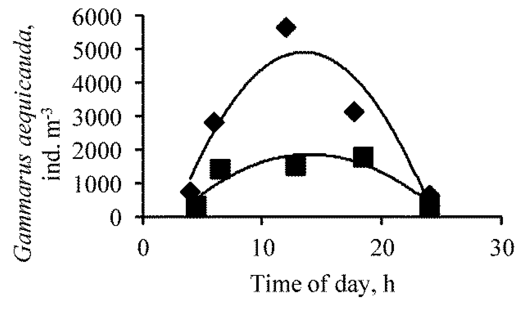
The number of G. aequicauda varied from 640 ind. m−3 (00:00) to 5660 ind. m−3 (12:00), on average 2600 ind. m−3 (CV = 0.793) at site 1 near the windward coast. At site 3, the abundance of G. aequicauda varied from 320 ind. m−3 (4:30) to 1780 ind. m−3 (18:45), on average 1076 ind. m−3 (CV = 0.645). The average abundance at the two sites differed significantly (p = 0.02). At site 1 and site 3, the dependence of the abundance of G. aequicauda on the time of day had a bell-shaped form with a maximum in the daytime (Figure 4).
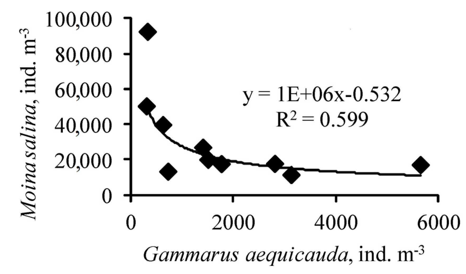
The average size of an individual was 3.1 mm (CV = 0.188) at site 1 and 2.9 (CV = 0.162) at site 3, and the differences were not significant. The average weight of crustaceans at the two sites did not differ, averaging 4.2 mg (CV = 0.652). The number of M. salina at site 1 varied from 11,300 ind. m−3 (17:45) to 39,600 ind. m−3 (00:30), on average 19,732 ind. m−3 (CV = 0.578). At site 3, its abundance varied from 17,500 ind. m−3 (18:20) to 92,400 ind. m−3 (00:00), on average 41,360 ind. m−3 (CV = 0.757). There is a significant (p = 0.005) negative relationship between the numbers of Moina and Gammarus (Figure 5).
The average abundance of E. mareotica at sites 1 and 3 was 625 ind. m−3 (CV = 1.095) and 1120 ind. m−3 (CV = 1.458), respectively. The remaining few species were encountered irregularly and in much smaller numbers, so are not discussed in this article.
On 14 September 2021, from 13:00 to 14:00 (the day before the day-long investigation), studies were carried out both on free-water sites 1 and 3 and in Ruppia thickets at site 2, the same as on 15 September 2021, and site 4 (near site 3). The sites differed from each other in the density of Ruppia shoots; at site 2, there were 3050 ind. m−2, and at site 4 there were 780 ind. m−2. The wind at that time was westerly, with a speed of 3 m s−1, i.e., sites 3 and 4 were at the windward coast, and sites 1 and 2 were at the leeward side. The total zooplankton abundance at site 1 was 20,840 ind. m−3, and at site 3, it was higher than 61,860 ind. m−3. The G. aequicauda abundance was 1740 ind. m−3 and 1620 ind. m−3 at sites 1 and 3, respectively. Differences for Moina were more pronounced, 18,800 ind. m−3 and 59,700 ind. m−3 at sites 1 and 3, respectively. Ostracoda was also more abundant at the third site (540 ind. m−3) than at the first site (300 ind. m−3).
In the Ruppia thickets, the picture was different, and the total zooplankton abundance at site 2 near the windward coast was 102,600 ind. m−3, and at site 4, it was 89,150 ind. m−3. The abundance of G. aequicauda was also higher at site 2 (87,000 ind. m−3) than at site 4 (15,300 ind. m−3). M. salina had the opposite picture; there were fewer individuals at 11,300 ind. m−3 at site 2 than the 72,900 ind. m−3 at site 4. The number of E. mareotica and C. retrogressus was higher at the 2nd site, 3500 ind. m−3 and 700 ind. m−3, respectively, than at the 4th site, where it was 500 ind. m−3 and 200 ind. m−3. Near the windward coast, the total abundance of all animals, except for M. salina, was higher. It should also be noted that the abundance of all species, except for M. salina, was higher in Ruppia thickets than in their absence. Benthic samples were not taken on 14–16 September, but they were taken at sites 1 and 2 on 12 September 2021. The largest number was of chironomid larvae. The abundance of chironomid larvae in Ruppia thickets was 1400 ind. m−2, some lower than outside the thickets, 1880 ind. m−2.
Using data on the animal abundance, oxygen consumption by the zoocenosis was calculated and given in Table 1. Using the average values for individual sites, the authors calculated the average share of animals in the total oxygen consumption (oxygen consumption by all animals/total oxygen consumption) 100%: at site 1, it was 4%, at site 3–5%, and at site 2 (with Ruppia thickets)—21%. The contribution of planktonic animals to the total oxygen consumption by zoocenosis was 26% and 28% at sites 1 and 3, respectively, and at sites 2 and 4 with Ruppia thickets, the contribution of planktonic animals was higher, 87% and 75%, respectively (Table 1).
Calculated according to the results of the study, the balance of oxygen in the daytime and at night at three sites is presented in Table 2. The daily production of oxygen during photosynthesis averaged 27.3 mgO L−1 day−1 (CV = 0.354); the highest values were noted at the windward site of 37.9 mgO L−1 day−1, and the lowest—at the leeward site of 19 mgO L−1 day−1. The least variable value was the total respiration of the community per day, on average 15.9 mgO L−1 day−1 (CV = 0.041). It averaged 63% (CV = 0.041) of the created primary production. The contribution of animals to the total oxygen consumption of the community was small, averaging 5% (CV = 0.693). The largest contribution of animals was noted in the thickets of Ruppia, 9%. The daily release of oxygen into the atmosphere was 6.1 mgO L−1 day−1, and it was the most variable element in the oxygen balance (CV = 1.483). The maximum amount was noted at site 1 near the windward coast 16.4 mgO L−1 day−1 or 46% of the primary production, at site 2, Ruppia thickets near the windward coast, −1.8 mgO L−1 day−1 or about 10% of the primary production, and at site 3—only 0.1 mgO L−1 day−1 or less than 5% of the total primary production.
4. Discussion
The obtained values of total primary production (average 27.3 mgO L−1 h−1) and chlorophyll a concentration (from 2 to 18.8 µg L−1) indicate that the lake is in a eutrophic state, and phytoplankton blooms were periodically observed within it [35,46]. The last bloom was noted after these observations, and a Microcystis concentration of 33.4 million cells L−1 was observed on 17 October 2021, during the period of the mass die-off and decomposition of Ruppia [46]. Despite the small size of the lake, the distribution of chlorophyll a concentration, and primary production in it was not uniform. The absence of a significant correlation between the concentration of chlorophyll a and the concentration of dissolved oxygen suggests that other factors intervene in the amount of dissolved oxygen, such as the turbulence generated by the wind and the presence of macrophytes, which are releasing oxygen to the water but are not recorded in chlorophyll a concentrations. The maximum average daily values of both parameters were recorded at site 2, where there were Ruppia thickets. The maximum range of diurnal fluctuations in oxygen concentration and the minimum range of fluctuations in chlorophyll a concentration were also noted here. This is usually typical for areas with the intensive development of macrophytes [17,19]. At sites without Ruppia thickets, the values for oxygen near the windward and leeward coasts did not differ significantly. However, the chlorophyll a concentration on average per day was 24% higher near the windward coast than near the leeward one. This is quite understandable, taking into account the wind transfer of all suspended particles, including phytoplankton, and their concentrations near the windward coast. Previously, similar differences between the windward and leeward shores were noted in the hypersaline Sivash lagoon [47].
Differences in the concentration of suspended matter near the two coasts were also due to the influence of the wind. At the same time, in areas without Ruppia thickets, the differences (much higher near the windward coast) were significant in the period from about 10:00 to 18:30 (15 September 2021), when the wind speed varied from 4 to 9 m s−1, and then later, at a lower wind speed, these differences were absent. Given the relatively low proportion of chlorophyll in TSS, it can be assumed that the main portion of particulate matter entered the water due to the resuspension of bottom sediments. Judging by the dynamics of differences in this parameter near the windward and leeward shores, it can be assumed that the wind resuspension of bottom sediments occurs in the lake at a wind speed of more than 4 m s−1. In the thickets of Ruppia, as well as other macrophytes, the critical value of the wind speed at which the resuspension of bottom sediments begins increases [48,49,50]. In our case, this phenomenon was weakly expressed.
The total abundance of zooplankton both on 15 September 2021, and 14 September 2021 was significantly higher near the leeward coast, which may seem illogical at first glance. However, this apparent contradiction can be removed when considering individual species. The abundance of G. aequicauda on both days was higher near the windward coast, while the abundance of M. salina and E. mareotica was higher near the leeward coast. G. aequicauda is a facultative predator that intensively consumes small plankton animals, including M. salina and E. mareotica [34]. Previously, experimental data were obtained on the intensity of Moina consumption by G. aequicauda [34]. Using them, the authors calculated how many Moina can be eaten by G. aequicauda per hour with the observed number of individuals near the windward coast: the number was 11,770 ind. m−3 h−1. The concentration of G. aequicauda by the wind near the windward shore led to more intense prey grazing, which led to a decrease in prey numbers. This masked the effect of wind on M. salina and E. mareotica, and, in this case, the effect of predation on the number of prey was stronger than that of wind. As the total number of prey was much higher than that of G. aequicauda, this resulted in a higher total abundance of zooplankton near the leeward rather than the windward coast. At the same time, in this case, it is difficult to separate the influence of two factors on the number of Moina—wind and predation by Gammarus. The numbers of bentho-planktonic Ostracoda and Harpacticoida were also higher near the windward coast. In this case, it is difficult to say what effect the wind had on the horizontal transport of animals and/or on their migration between the bottom and plankton. It should be noted that wind can affect different species and age cohorts of animals [47,51] because wind can also affect the transition of bento-plankton animals from plankton to the benthos and vice versa.
In this study, it was found that the role of animals in oxygen consumption by a community, and hence in the oxidation of organic matter, is not large, from 3 to 9% (Table 2), which is consistent with previously obtained values [23,24]. At the same time, this is somewhat less than in freshwater bodies [52]. Thus, more than 90% of total oxygen by community consumption was attributed to algae, marine grass, and bacteria with protozoa in plankton and benthos.
The oxygen balance calculated from the results of the study at three sites is presented in Table 1 and Table 2. Oxygen production during photosynthesis per day exceeded its consumption by the lake community at all sites. On average, 19% of the oxygen released during photosynthesis went into the atmosphere, while from site to site, this proportion varied significantly, from 4 to 46%. This indicator, as shown by our data, is affected by wind and the absence/presence of thickets of underwater plants. From these results, the conclusion follows that the ecosystem of a small hypersaline lake is not balanced in terms of the oxygen cycle, as well as carbon, which was also noted earlier [23,24]. In this regard, it is interesting to consider the question of the effect of salinity on the balance of the oxygen cycle in shallow lakes. To do this, it is necessary to analyze Equations (1) and (3) together. Substituting Equation (1) into Equation (3) and get:
F = k (DOt − 8.268 e−0.006S)/Zmix,
As follows from Equation (34), if the ratio k/Zmix is constant, the process of oxygen released into the atmosphere by the water body can proceed at 25 °C, if DOt > 8.268 e−0.006S. At the same time, with an increase in salinity, the process begins with a lower oxygen concentration and goes faster. For example, at an oxygen concentration of 9 mg L−1, at a salinity of 0 g L−1, the rate of oxygen loss by the lake can be approximately 0.7 k/Zmix mg O2 m−2 h−1, at 20 g L−1–1.7 k/Zmix mg O2 m−2 h−1, at 100 g L−1–4.5 k/Zmix mg O2 m−2 h−1, and at 200 g L−1–6.5 k/Zmix mg O2 m−2 h−1. At the same time, it should be recalled that the saturating oxygen concentration at a salinity of 0 g L−1 is 8.3 mg L−1, at a salinity of 100 g L−1 is 4.5 mg L−1, and at 200 g L−1 is only 2.5 g L−1. These values show how significantly the increase in salinity may increase the loss of oxygen in a shallow lake. An increase in the loss of oxygen in a water body with an increase in salinity at a similar level of primary production leads to the fact that a smaller proportion of the produced organic matter may be oxidized in plankton. Consequently, most of it can sink to the bottom, as in most lakes [52]. An increase in salinity also leads to a decrease in the oxygen diffusion coefficient [30], which also contributes to the frequent formation of hypo- and anoxic conditions near the bottom of hypersaline water bodies [25,53]. Under such conditions, the rate of the bacterial destruction of algodetritus is significantly reduced [54,55]. With an increase in salinity, more organic matter may thus be buried in bottom sediments, and carbon can be eliminated from the biotic cycle. A similar conclusion was drawn from several other data previously, noting the important role of hypersaline water bodies as natural mechanisms that prevent the growth of CO2 in the atmosphere [22,23,24]. On the other hand, a generalization of a large amount of data showed that, in most analyzed case studies, the release of CO2 by lakes increased with an increase in salinity [20,21]. Such a contradiction in the data and conclusions from them suggests that this question is not very simple and does not have a monosemantic answer. However, the hypersaline water bodies are highly likely a net sink of carbon, rather than a source for the atmosphere.
Previously, it was noted that the diurnal variability of several abiotic parameters (temperature, pH, Eh) in hypersaline water bodies is higher than in less saline ones [23,25]. Based on both our data and the analysis of Equation (34), it can be argued that the daily range of changes in the oxygen concentration in the lakes must inevitably increase with increasing salinity dropping episodically to zero. The daily course of PAR entry into the lake changes significantly from season to season, determining both the process of primary production and the daily course of oxygen concentration. Therefore, the results obtained in one season cannot always be correctly extrapolated to other seasons. It should probably be assumed that, in some seasons the lake can absorb and in others release, O2 and CO2. Further research is needed in this direction with the accumulation and analysis of data on specific lakes in different seasons.
5. Conclusions
A joint analysis of new and published data allows, without going into details, one to draw a general conclusion. Only knowledge of the daily dynamics of various ecosystem parameters makes it possible to assess the production status of the lake. If the daily rhythms are unknown, it is difficult to judge the real state and dynamics of aquatic ecosystems by singular measurements of parameters. When studying diurnal rhythms in small lakes, diurnal fluctuations in wind speed and direction also cannot be overlooked. Considering the daily dynamics of various ecosystem parameters, as in our case, it is necessary to take into account the complex nature of their nonlinear interactions with each other. Discussing our data, primarily equations, it should be noted that they are only particular implementations of general patterns in the interaction of many external and intra-ecosystem factors, causes, and effects. They cannot be absolutized; they are only steps towards understanding the real complexity of multiscale ecosystem dynamics.
Author Contributions
Conceptualization, N.S. and E.A.; methodology, N.S. and A.P.; formal analysis, N.S., E.A., A.L. and V.Y.; investigation, E.A., A.L., A.P. and V.Y.; writing—original draft preparation, N.S.; writing—review and editing, N.S., E.A., A.L., A.P. and V.Y.; project administration, E.A.; funding acquisition, E.A. All authors have read and agreed to the published version of the manuscript.
Funding
Field study of environmental parameters, data analysis, and the writing of this manuscript were supported by the Russian Science Foundation (grant 18-16-00001); the field study of the community composition was conducted in the framework of the state assignment of the A.O. Kovalevsky Institute of Biology of the Southern Seas of RAS (No 121041500203-3); TSS measurements and analysis were conducted in the framework by the state assignment of the Marine Hydrophysical Institute of RAS (No 0555-2021-0003).
Institutional Review Board Statement
Not applicable.
Informed Consent Statement
Not applicable.
Data Availability Statement
All data used in this study are available upon request from the corresponding author.
Acknowledgments
The authors are grateful to Bindy Datson (Australia) for her selfless work in improving the English of this manuscript.
Conflicts of Interest
The authors declare no conflict of interest.
References
- Holling, C.S. Understanding the complexity of economic, ecological, and social systems. Ecosystems 2001, 4, 390–405. [Google Scholar] [CrossRef]
- Green, D.G.; Sadedin, S. Interactions matter—Complexity in landscapes and ecosystems. Ecol. Complex. 2005, 2, 117–130. [Google Scholar] [CrossRef]
- Allen, C.R.; Angeler, D.G.; Garmestani, A.S.; Gunderson, L.H.; Holling, C.S. Panarchy: Theory and application. Ecosystems 2014, 17, 578–589. [Google Scholar] [CrossRef] [Green Version]
- Shadrin, N.V. The alternative saline lake ecosystem states and adaptive environmental management. J. Oceanol. Limnol. 2018, 36, 2010–2017. [Google Scholar] [CrossRef]
- Stross, R.G.; Chisholm, S.W.; Downing, T.A. Causes of daily rhythms in photosynthetic rates of phytoplankton. Biol. Bull. 1973, 145, 200–209. [Google Scholar] [CrossRef]
- Andrew, T.E.; Cabrera, S.; Montecino, V. Diurnal changes in zooplankton respiration rates and the phytoplankton activity in two Chilean lakes. Hydrobiologia 1989, 175, 121–135. [Google Scholar] [CrossRef]
- Forsberg, B.R.; Melack, J.M.; Richey, J.E.; Pimentel, T.P. Regional and seasonal variability in planktonic photosynthesis and planktonic community respiration in Amazon floodplain lakes. Hydrobiologia 2017, 800, 187–206. [Google Scholar] [CrossRef]
- Baxa, M.; Musil, M.; Kummel, M.; Hanzlík, P.; Tesařová, B.; Pechar, L. Dissolved oxygen deficits in a shallow eutrophic aquatic ecosystem (fishpond)–Sediment oxygen demand and water column respiration alternately drive the oxygen regime. Sci. Total Environ. 2021, 766, 142647. [Google Scholar] [CrossRef]
- Winberg, G.G.; Yarovitsina, L.I. Daily fluctuations in the amount of dissolved oxygen as a method for measuring the value of the primary production of water bodies. Tr. Limnol. Stantsii V Kosine 1939, 22, 128–143. (In Russian) [Google Scholar]
- Winberg, G.G. On the measurement of the rate of exchange of oxygen between a water basin and atmosphere. CR Acad. Sci. URSS 1940, 26, 666–669. [Google Scholar]
- Staehr, P.A.; Bade, D.; Van de Bogert, M.C.; Koch, G.R.; Williamson, C.; Hanson, P.; Cole, J.J.; Kratz, T. Lake metabolism and the diel oxygen technique: State of the science. Limnol. Oceanogr. Methods 2010, 8, 628–644. [Google Scholar] [CrossRef]
- Lovett, G.M.; Cole, J.J.; Pace, M.L. Is net ecosystem production equal to ecosystem carbon accumulation? Ecosystems 2006, 9, 152–155. [Google Scholar] [CrossRef]
- Hall, R.O., Jr.; Beaulieu, J.J. Estimating autotrophic respiration in streams using daily metabolism data. Freshw. Sci. 2013, 32, 507–516. [Google Scholar] [CrossRef]
- Bas-Silvestre, M.; Quintana, X.D.; Compte, J.; Gascón, S.; Boix, D.; Antón-Pardo, M.; Obrador, B. Ecosystem metabolism dynamics and environmental drivers in Mediterranean confined coastal lagoons. Estuar. Coast. Shelf Sci. 2020, 245, 106989. [Google Scholar] [CrossRef]
- Tolkamp, H.H.; Van Vierssen, W.; Knoben, R.A. Oxygen variation in Dutch water types in relation to biological water quality criteria. Int. Ver. Theor. Angew. Limnol. Verh. 1991, 24, 2095–2099. [Google Scholar] [CrossRef]
- Witek, Z.; Jarosiewicz, A.; Cyra, M. Peculiarities of pelagic community metabolism in small dimictic lakes as demonstrated by daily changes of oxygen vertical distribution. Pol. J. Environ. Stud. 2013, 22, 933–943. [Google Scholar]
- Kragh, T.; Andersen, M.R.; Sand-Jensen, K. Profound afternoon depression of ecosystem production and nighttime decline of respiration in a macrophyte-rich, shallow lake. Oecologia 2017, 185, 157–170. [Google Scholar] [CrossRef]
- Palshin, N.I.; Efremova, T.V.; Zdorovennova, G.E.; Gavrilenko, G.G.; Zdorovennov, R.E.; Terzhevik, A.Y.; Volkov, S.Y.; Bogdanov, S.R. Diurnal dynamics of dissolved oxygen in a small mesotrophic lake during spring under-ice warming. Izv. Rus. Geogr. Obs. 2019, 151, 27–39. (In Russian) [Google Scholar] [CrossRef]
- Sand-Jensen, K.; Andersen, M.R.; Martinsen, K.T.; Borum, J.; Kristensen, E.; Kragh, T. Shallow plant-dominated lakes–extreme environmental variability, carbon cycling and ecological species challenges. Ann. Bot. 2019, 124, 355–366. [Google Scholar] [CrossRef] [Green Version]
- Duarte, C.M.; Prairie, Y.T.; Montes, C.; Cole, J.J.; Striegl, R.; Melack, J.; Downing, J.A. CO2 emissions from saline lakes: A global estimate of a surprisingly large flux. J. Geophys. Res. Biogeosci. 2008, 113, G04041. [Google Scholar] [CrossRef] [Green Version]
- Yan, F.; Sillanpää, M.; Kang, S.; Aho, K.S.; Qu, B.; Wei, D.; Li, X.; Li, C.; Raymond, P.A. Lakes on the Tibetan Plateau as conduits of greenhouse gases to the atmosphere. J. Geophys. Res. Biogeosci. 2018, 123, 2091–2103. [Google Scholar] [CrossRef]
- Jellison, R.; Anderson, R.F.; Melack, J.M.; Heil, D. Organic matter accumulation in sediments of hypersaline Mono Lake during a period of changing salinity. Limnol. Oceanogr. 1996, 41, 1539–1544. [Google Scholar] [CrossRef]
- Shadrin, N.; Zheng, M.; Oren, A. Past, present and future of saline lakes: Research for global sustainable development. Chin. J. Oceanol. Limnol. 2015, 33, 1349–1353. [Google Scholar] [CrossRef]
- Prazukin, A.V.; Anufriieva, E.V.; Shadrin, N.V. Photosynthetic activity of filamentous green algae mats hypersaline lake Chersonesskoye (Crimea). Vestn. TVER Univ. Ser. Biol. I Ecol. 2019, 2, 87–102. (In Russian) [Google Scholar]
- Shadrin, N.; Anufriieva, E. Ecosystems of hypersaline waters: Structure and trophic relations. Zhurnal Obs. Biol. 2018, 79, 418–427. [Google Scholar]
- Saccò, M.; White, N.E.; Harrod, C.; Salazar, G.; Aguilar, P.; Cubillos, C.F.; Meredith, K.; Baxter, B.K.; Oren, A.; Anufriieva, E.; et al. Salt to conserve: A review on the ecology and preservation of hypersaline ecosystems. Biol. Rev. 2021, 96, 2828–2850. [Google Scholar] [CrossRef] [PubMed]
- Gat, J.R.; Shatkay, M. Gas exchange with saline waters. Limnol. Oceanogr. 1991, 36, 988–997. [Google Scholar] [CrossRef]
- Sherwood, J.E.; Stagnitti, F.; Kokkinn, M.J.; Williams, W.D. Dissolved oxygen concentrations in hypersaline waters. Limnol. Oceanogr. 1991, 36, 235–250. [Google Scholar] [CrossRef]
- Debelius, B.; Gomez-Parra, A.; Forja, J.M. Oxygen solubility in evaporated seawater as a function of temperature and salinity. Hydrobiologia 2009, 632, 157–165. [Google Scholar] [CrossRef]
- Shadrin, N.V. Hypersaline lakes as polyextreme habitats for life. In Introduction to Salt Lake Sciences; Zheng, M., Deng, T., Oren, A., Eds.; Science Press: Beijing, China, 2018; pp. 180–187. [Google Scholar]
- Anufriieva, E.; Hołyńska, M.; Shadrin, N. Current invasions of Asian Cyclopid species (Copepoda: Cyclopidae) in Crimea, with taxonomical and zoogeographical remarks on the hypersaline and freshwater fauna. Ann. Zool. 2014, 64, 109–130. [Google Scholar] [CrossRef]
- Soulié, T.; Mas, S.; Parin, D.; Vidussi, F.; Mostajir, B. A new method to estimate planktonic oxygen metabolism using high-frequency sensor measurements in mesocosm experiments and considering daytime and nighttime respirations. Limnol. Oceanogr. Methods 2021, 19, 303–316. [Google Scholar] [CrossRef]
- Shadrin, N.; Yakovenko, V.; Anufriieva, E. Suppression of Artemia spp. (Crustacea, Anostraca) populations by predators in the Crimean hypersaline lakes: A review of the evidence. Int. Rev. Hydrobiol. 2019, 104, 5–13. [Google Scholar] [CrossRef] [Green Version]
- Shadrin, N.; Yakovenko, V.; Anufriieva, E. Gammarus aequicauda and Moina salina in the Crimean saline waters: New experimental and field data on their trophic relation. Aquac. Res. 2020, 51, 3091–3099. [Google Scholar] [CrossRef]
- Shadrin, N.V.; Yakovenko, V.A.; Anufriieva, E.V. Appearance of a new species of Cladocera (Anomopoda, Chydoridae, Bosminidae) in the hypersaline Moynaki Lake, Crimea. Biol. Bull. 2021, 48, 934–937. [Google Scholar] [CrossRef]
- Müller, P.H.; Neuman, P.; Storm, R. Tafeln der Mathematischen Statistik; VEB Fachbuchverlag: Leipzig, Germany, 1979; 276p. [Google Scholar]
- Thode, H.C. Testing for Normality; Marcel Dekker Inc.: New York, NY, USA, 2002; 368p. [Google Scholar]
- Cole, J.J.; Bade, D.L.; Bastviken, D.; Pace, M.L.; Van de Bogert, M. Multiple approaches to estimating air-water gas exchange in small lakes. Limnol. Oceanogr. Methods 2010, 8, 285–293. [Google Scholar] [CrossRef]
- Geider, R.J.; Osborne, B.A. Respiration and microalgal growth: A review of the quantitative relationship between dark respiration and growth. New Phytol. 1989, 112, 327–341. [Google Scholar] [CrossRef]
- Ivleva, I.I. The Temperature of the Environment and the Rate of Energy Metabolism Aquatic Animals; Naukova Dumka: Kiyev, Ukraine, 1981; 231p. (In Russian) [Google Scholar]
- Rasmusson, L.M.; Gullström, M.; Gunnarsson, P.C.; George, R.; Björk, M. Estimation of a whole plant Q10 to assess seagrass productivity during temperature shifts. Sci. Rep. 2019, 9, 12667. [Google Scholar] [CrossRef] [Green Version]
- Gudasz, C.; Karlsson, J.; Bastviken, D. When does temperature matter for ecosystem respiration? Environ. Res. Commun. 2021, 3, 121001. [Google Scholar] [CrossRef]
- Sushchenya, L.M. Intensity of Respiration of Crustaceans; Naukova Dumka: Kyiv, Ukraine, 1972; 196p. (In Russian) [Google Scholar]
- Balushkina, E.V. The Functional Significance of Chironomid Larvae in Continental Reservoirs; Nauka: Leningrad, Russia, 1987; 179p. (In Russian) [Google Scholar]
- Alimov, A.F. An Introduction to Production Hydrobiology; Gidrometeoizdat: Leningrad, Russia, 1989; 152p. (In Russian) [Google Scholar]
- Yakovenko, V.; Shadrin, N.; Anufriieva, E. The prawn Palaemon adspersus in the hypersaline Lake Moynaki (Crimea): Ecology, long-term changes, and prospects for aquaculture. Water 2022, 14, 2786. [Google Scholar] [CrossRef]
- Anufriieva, E.; Shadrin, N. The long-term changes in plankton composition: Is Bay Sivash transforming back into one of the world’s largest habitats of Artemia sp. (Crustacea, Anostraca)? Aquac. Res. 2020, 51, 341–350. [Google Scholar] [CrossRef]
- Horppila, J.; Nurminen, L. Effects of submerged macrophytes on sediment resuspension and internal phosphorus loading in Lake Hiidenvesi (southern Finland). Water Res. 2003, 37, 4468–4474. [Google Scholar] [CrossRef]
- Widdows, J.; Pope, N.D.; Brinsley, M.D.; Asmus, H.; Asmus, R.M. Effects of seagrass beds (Zostera noltii and Z. marina) on near-bed hydrodynamics and sediment resuspension. Mar. Ecol. Prog. Ser. 2008, 358, 125–136. [Google Scholar] [CrossRef] [Green Version]
- Zheng, X.; Zhang, K.; Yang, T.; He, Z.; Shu, L.; Xiao, F.; Wu, Y.; Wang, B.; Yu, H.; Yan, Q. Sediment resuspension drives protist metacommunity structure and assembly in grass carp (Ctenopharyngodon idella) aquaculture ponds. Sci. Total Environ. 2021, 764, 142840. [Google Scholar] [CrossRef] [PubMed]
- Anufriieva, E.; Kolesnikova, E.; Revkova, T.; Latushkin, A.; Shadrin, N. Human-induced sharp salinity changes in the world’s largest hypersaline lagoon Bay Sivash (Crimea) and their effects on the ecosystem. Water 2022, 14, 403. [Google Scholar] [CrossRef]
- Alimov, A.F. Elements of aquatic ecosystem function theory. Proc. Zool. Inst. Russ. Acad. Sci. 2000, 283, 2–147. [Google Scholar]
- Shadrin, N.V.; Anufriieva, E.V. Climate change impact on the marine lakes and their Crustaceans: The case of marine hypersaline Lake Bakalskoye (Ukraine). Turk. J. Fish. Aquat. Sci. 2013, 13, 603–611. [Google Scholar] [CrossRef]
- Middelburg, J.J.; Levin, L.A. Coastal hypoxia and sediment biogeochemistry. Biogeosciences 2009, 6, 1273–1293. [Google Scholar] [CrossRef] [Green Version]
- Jessen, G.L.; Lichtschlag, A.; Ramette, A.; Pantoja, S.; Rossel, P.E.; Schubert, C.J.; Struck, U.; Boetius, A. Hypoxia causes preservation of labile organic matter and changes seafloor microbial community composition (Black Sea). Sci. Adv. 2017, 3, e1601897. [Google Scholar] [CrossRef]
Figure 1.
The scheme of Lake Moynaki and studied sites ((A) the Crimean scale; (B) the Lake Moynaki scale). Sites 1, 2, and 3 were studied from 15 to 16 September, and site 4 was studied only once on 14 September (zooplankton and benthos).
Figure 1.
The scheme of Lake Moynaki and studied sites ((A) the Crimean scale; (B) the Lake Moynaki scale). Sites 1, 2, and 3 were studied from 15 to 16 September, and site 4 was studied only once on 14 September (zooplankton and benthos).

Figure 2.
Diurnal course of photosynthetically active radiation (PAR) in the upper layer of the water column in Lake Moynaki during 15–16 September 2021.
Figure 2.
Diurnal course of photosynthetically active radiation (PAR) in the upper layer of the water column in Lake Moynaki during 15–16 September 2021.

Figure 3.
Diurnal changes of the chlorophyll a content in three stations (squares—1st station, rhombuses—2nd station, triangles—3rd station) of Lake Moynaki during 15–16 September 2021.
Figure 3.
Diurnal changes of the chlorophyll a content in three stations (squares—1st station, rhombuses—2nd station, triangles—3rd station) of Lake Moynaki during 15–16 September 2021.

Figure 4.
Diurnal changes of Gammarus aequicauda abundance in water columns in site 1 (rhombuses) and site 3 (squares) of Lake Moynaki during 15–16 September 2021.
Figure 4.
Diurnal changes of Gammarus aequicauda abundance in water columns in site 1 (rhombuses) and site 3 (squares) of Lake Moynaki during 15–16 September 2021.

Figure 5.
Relationship between changes in the abundance of Gammarus aequicauda and Moina salina in Lake Moynaki during 15–16 September 2021.
Figure 5.
Relationship between changes in the abundance of Gammarus aequicauda and Moina salina in Lake Moynaki during 15–16 September 2021.


Table 1.
Calculated indicators of oxygen consumption by zoocenosis in Lake Moynaki, 15–16 September 2021.
Table 1.
Calculated indicators of oxygen consumption by zoocenosis in Lake Moynaki, 15–16 September 2021.
| Date, Time | Oxygen Consumption, mg O2 h−1 m−3 | ||||||
|---|---|---|---|---|---|---|---|
| Gammarus aequicauda | Moina salina | Eucypris mareotica | Total Zooplankton | Chironomid Larvae | Total Zoocenosis | Total Zooplankton/Total Zoocenosis | |
| Outside Ruppia thickets | |||||||
| Station 1 | |||||||
| 14 September 2021 13:00 | 3.14 | 2.33 | 0.08 | 5.55 | 14.14 | 19.69 | 0.28 |
| 15 September 2021 12:00 | 6.58 | 1.07 | 0.01 | 7.66 | 14.14 | 21.80 | 0.35 |
| 15 September 2021 17:53 | 5.57 | 1.00 | 0.08 | 6.65 | 14.14 | 20.79 | 0.32 |
| 16 September 2021 00:30 | 1.19 | 2.70 | <0.01 | 4.60 | 14.14 | 18.74 | 0.25 |
| 16 September 2021 04:00 | 2.56 | 0.73 | 0 | 3.29 | 14.14 | 17.43 | 0.19 |
| 16 September 2021 06:04 | 5.08 | 1.00 | 0.05 | 6.85 | 14.14 | 20.99 | 0.33 |
| Average | 4.02 | 1.47 | 0.04 | 5.77 | 14.14 | 19.91 | 0.26 |
| CV | 0.510 | 0.560 | 1.025 | 0.280 | - | 0.081 | 0.208 |
| Station 3 | |||||||
| 14 September 2021 14:00 | 2.93 | 5.84 | 0.05 | 8.82 | 14.14 | 22.96 | 0.38 |
| 15 September 2021 12:43 | 2.46 | 1.76 | 0.01 | 4.23 | 14.14 | 18.37 | 0.23 |
| 15 September 2021 18:27 | 3.96 | 1.01 | 0.02 | 4.99 | 14.14 | 19.13 | 0.26 |
| 16 September 2021 00:01 | 0.90 | 7.00 | 0 | 7.9 | 14.14 | 22.04 | 0.36 |
| 16 September 2021 04:28 | 1.21 | 3.71 | 0 | 4.92 | 14.14 | 19.06 | 0.26 |
| 16 September 2021 06:32 | 1.61 | 1.56 | 0.12 | 3.29 | 14.14 | 17.43 | 0.19 |
| Average | 2.18 | 3.48 | 0.03 | 5.69 | 14.14 | 19.83 | 0.28 |
| CV | 0.532 | 0.713 | 1.390 | 0.382 | - | 0.110 | 0.266 |
| Inside Ruppia thickets | |||||||
| Station 2 | |||||||
| 14 September 2021 13:10 | 66.40 | 0.64 | 0.56 | 67.60 | 10.52 | 78.12 | 0.87 |
| Station 4 | |||||||
| 14 September 2021 14:10 | 30.26 | 0.74 | 0.09 | 31.09 | 10.52 | 41.61 | 0.75 |
| Average | 48.33 | 0.69 | 0.33 | 49.35 | 10.52 | 59.87 | 0.81 |
| CV | 0.529 | 0.102 | 1.023 | 0.523 | - | 0.431 | 0.105 |
Note: CV—coefficient of variation.
Table 2.
Calculated indicators of the oxygen balance (mg O2 m−3) in Lake Moynaki, 15–16 September 2021.
Table 2.
Calculated indicators of the oxygen balance (mg O2 m−3) in Lake Moynaki, 15–16 September 2021.
| GPP | R | Ra | Ra/R | Fla | Fal | Fla − Fal | Fla/GPP | R/GPP | |
|---|---|---|---|---|---|---|---|---|---|
| Day time | |||||||||
| Station 1 | 37.9 | 9.7 | 0.24 | 0.03 | 17.6 | 0 | 0.48 | 0.25 | |
| Station 2 | 25 | 10.7 | 0.72 | 0.07 | 1.9 | 0 | 0.08 | 0.43 | |
| Station 3 | 19.0 | 10.1 | 0.21 | 0.04 | 0.7 | 0 | 0.04 | 0.53 | |
| Average/CV | 27.3/ 0.354 | 10.1/ 0.054 | 0.39/ 0.735 | 0.04/ 0.496 | 6.7/ 1.398 | 0.40/ 0.352 | |||
| Dark time (night) | |||||||||
| Station 1 | 0 | 5.6 | 0.24 | 0.04 | 0 | 1.2 | −1.2 | ||
| Station 2 | 0 | 5.9 | 0.72 | 0.12 | 0 | 0.96 | −0.96 | ||
| Station 3 | 0 | 5.5 | 0.21 | 0.04 | 0 | 0.72 | −0.72 | ||
| Average/CV | 0 | 5.7/ 0.037 | 0.39/ 0.735 | 0.07/ 0.693 | 0 | 0.96/ 0.250 | −0.96/ 0.250 | ||
| Day and night | |||||||||
| Station 1 | 37.9 | 15.2 | 0.4778 | 0.03 | 17.6 | 1.2 | 16.4 | 0.46 | 0.40 |
| Station 2 | 25 | 16.6 | 1.4368 | 0.09 | 1.9 | 1.0 | 1.8 | 0.08 | 0.66 |
| Station 3 | 19.0 | 15.6 | 0.4184 | 0.03 | 0.8 | 0.7 | 0.1 | 0.04 | 0.82 |
| Average/CV | 27.3/ 0.354 | 15.9/ 0.041 | 0.78/ 0.735 | 0.05/ 0.693 | 6.7/ 1.398 | 1.00/ 0.250 | 6.1/ 1.483 | 0.19/ 1.199 | 0.63/ 0.338 |
Notes: GPP is the gross primary production; R is the total ecosystem respiration; Ra is the total oxygen consumption (respiration) by zoocenosis; Fla is the oxygen flux from the lake to the atmosphere; Fal is the oxygen flux from the atmosphere to the lake; CV is the coefficient of variation.
Publisher’s Note: MDPI stays neutral with regard to jurisdictional claims in published maps and institutional affiliations. |
© 2022 by the authors. Licensee MDPI, Basel, Switzerland. This article is an open access article distributed under the terms and conditions of the Creative Commons Attribution (CC BY) license (https://creativecommons.org/licenses/by/4.0/).
Share and Cite
MDPI and ACS Style
Shadrin, N.; Anufriieva, E.; Latushkin, A.; Prazukin, A.; Yakovenko, V. Daily Rhythms and Oxygen Balance in the Hypersaline Lake Moynaki (Crimea). Water 2022, 14, 3753. https://doi.org/10.3390/w14223753
AMA Style
Shadrin N, Anufriieva E, Latushkin A, Prazukin A, Yakovenko V. Daily Rhythms and Oxygen Balance in the Hypersaline Lake Moynaki (Crimea). Water. 2022; 14(22):3753. https://doi.org/10.3390/w14223753
Chicago/Turabian StyleShadrin, Nickolai, Elena Anufriieva, Alexander Latushkin, Alexander Prazukin, and Vladimir Yakovenko. 2022. "Daily Rhythms and Oxygen Balance in the Hypersaline Lake Moynaki (Crimea)" Water 14, no. 22: 3753. https://doi.org/10.3390/w14223753
Note that from the first issue of 2016, this journal uses article numbers instead of page numbers. See further details here.