Deep Learning Methods for Predicting Tap-Water Quality Time Series in South Korea

Abstract

South Korea currently lacks a real-time monitoring and anomaly detection system for detecting continuous tap water quality changes from the water source to faucet and pre-diagnosing hazards that threaten tap water safety. In this study, we constructed an accurate water quality prediction model that could comprehensively cover all water treatment facilities supplying tap water nationwide and verified the model using an integrated approach. To address the uncertainty of continuously changing water quality, we collected five years (2017–2021) of hourly water quality data from 33 large water purification plants and applied various deep learning techniques to construct an optimal prediction model. We repeated water quality prediction and evaluation over the following 24 h through a time series cross-validation of an untrained dataset of the previous five months. The optimized deep learning model achieved average and maximum prediction accuracy of 98.78 and 99.98%, respectively, and showed excellent performance in terms of the root mean squared error (0.0006), mean absolute error (0.0003), and Nash–Sutcliffe efficiency (0.9894). Thus, deep learning technology greatly improved the accuracy and efficiency of water quality prediction. The proposed model could provide prompt and accurate water quality information for large-scale water supply facilities nationwide and improve public health through the early diagnosis of water quality anomalies.

1. Introduction

In 2020, more than 50 million people in South Korea were supplied with tap water, accounting for 99.4% of the total population [1]. Following the treatment of raw water at 38 water treatment facilities, the Korea Water Resources Corporation (K-water) supplies 17.76 million tons of tap water per day to 113 major cities and industrial complexes nationwide through a vast water supply system, representing one of South Korea’s largest social infrastructures. However, if multiple water quality problems simultaneously occur within the system, damage can spread to several regions and impact public health and safety over a wide area; thus, effective water quality management is crucial. Recently, South Korea has suffered numerous water quality incidents related to tap water (reddish-brown water, water cut-offs, contamination with midge larvae, etc.), which has increased social distrust of the national water management system and further reduced tap water consumption [2,3]. To dispel this distrust, a real-time monitoring system is required that can promptly identify the continuously changing water quality conditions from the water source to faucet to pre-diagnose any hazards that may threaten tap water safety [3,4,5].

South Korea currently faces numerous challenges in terms of water resource management and water security. Currently, the foundations have been laid for integrated water management tailored to the characteristics of each water system, with extensive efforts made to resolve temporal and regional variability by establishing a multi-regional water supply system [6]. Additionally, a real-time water quality monitoring system was introduced to swiftly respond to changes in the environmental conditions of the water intake source, such as sudden changes in water quality indicated by pH, turbidity, and residual chloride. However, under the current system, a sensor failure or water quality problem can go unnoticed for several days or longer; this lack of a prompt response can drastically increase the number of complaints from residents.

To address these limitations and shift to a more proactive response system, a water quality prediction system that can prevent water quality accidents, manage the water quality environment, and protect water resources is needed [7,8]. However, few studies have conducted systematic analyses of water quality prediction systems for potable tap water. Moreover, South Korea is still lacking an accurate water quality prediction model that has been verified using an integrated approach and can comprehensively cover all water treatment facilities supplying tap water. Although South Korea has had a well-established water management infrastructure since the incident of prolonged reddish-brown water damage in Incheon in 2019, which was caused by an inadequate response to incidents, as well as similar incidents in several other regions, the country urgently requires a more advanced system that can predict water quality in tap water supply pipelines in real time, according to regional characteristics.

Accordingly, the goal of this study is to develop a deep learning-based real-time water quality prediction model for tap water that can cover the entire country, rather than being limited to a specific region. For this purpose, we used major water quality monitoring indicators measured hourly at water treatment centers managed by K-water, considering the water quality standards for drinking water prepared by the Ministry of Environment. Specifically, we collected five-and-a-half years (1 January 2017 to 31 May 2022) of hourly water quality data from 33 large water purification plants that produce and supply tap water throughout South Korea. Then, we conducted an in-depth analysis of nationwide tap water quality. The data included three water quality monitoring indicators: hydrogen ion concentration (pH), turbidity, and residual chloride. To identify each water quality indicator using the data collected from each water purification plant, we conducted pattern analysis, correlation analysis, and anomaly processing. Next, to predict the three water quality indicators in real time, we applied three deep learning techniques to construct an optimal model for accurately predicting water quality, namely long short-term memory (LSTM) [9], gated recurrent units (GRU) [10], and Sample Convolution and Interaction Networks (SCINet) architecture [11]. The autoregressive integrated moving average (ARIMA) model, which is widely used for time series prediction, was selected as the baseline model for comparison with the deep learning models. To address the uncertainty of continuously changing water quality, we combined actual tap water quality data sets from multiple regions nationwide, then developed deep learning models based on approximately five years of data from January 2017 to December 2021. We applied a time series cross-validation method to five months of data from January to May 2022 that were not used for training, then verified the generalization capacity of the developed model. The time series cross-validation method is an iterative process involving training with three days of data and then predicting water quality for the following 24 h. The prediction accuracy of the models was compared using the mean average error (MAE), root mean squared error (RMSE), and Nash–Sutcliffe efficiency (NSE).

According to the experimental results, the optimized deep learning-based neural network model achieved an average prediction accuracy of 98.78% and maximum prediction accuracy of 99.98%. In various real datasets of tap water quality, the model showed excellent performance in terms of MAE and RMSE, with minimum values of 0.0003 and 0.0006, respectively. These results show that deep learning techniques can greatly improve the accuracy and efficiency of predicting constantly changing water quality. The proposed deep learning model would provide real-time accurate water quality prediction information for 33 actual large water supply facilities throughout South Korea, enabling constant monitoring of continuously changing water quality conditions, which could help minimize the spread of damage through the early diagnosis of water quality anomalies.

The rest of this paper is structured as follows: Section 2 describes the current status of research on water quality prediction and potable tap water quality standards in South Korea. Section 3 describes data collection and preprocessing methods. Section 4 describes the exploratory data analysis. Section 5 describes the theory and construction of the proposed deep learning model. Section 6 presents the model training and validation and evaluates the predictive performance of the trained optimal model. Finally, Section 7 highlights the research findings and scope for future work.

2. Related Literature

2.1. Deep Learning-Based Methods

Previous water quality prediction studies have applied machine learning techniques such as random forest, eXtreme gradient boosting (XGBoost), support vector machine (SVM), and artificial neural networks (ANN). To predict the water quality index, Ahmed et al. [12] used a sequence of supervised machine learning algorithms based on four water quality parameters: temperature, turbidity, pH, and total dissolved solids. Among the applied algorithms, gradient boosting (learning rate of 0.1) and polynomial regression (order of 2) predicted the water quality index most efficiently, with MAE values of 1.9642 and 2.7273, respectively. Chen et al. [13] compared the water quality prediction performance of 10 learning models (seven traditional and three ensemble models) using big data of major rivers and lakes in China. They identified and verified major water parameters (dissolved oxygen (DO), chemical oxygen demand (COD), and NH3–N), which demonstrated the high specificity of permanent water quality. El Bilali and Taleb [14] developed eight machine learning models for predicting irrigation water quality in semi-arid regions using only two water parameters (conductivity and pH) as inputs. The results indicated that machine learning models could overcome several limitations of existing approaches when evaluating the suitability of water for agricultural purposes. Loos et al. [15] proposed a method for improving the accuracy of real-time water quality prediction, based on the parameters of water temperature, nutrients, and algae along the Yeongsan River in South Korea. They conducted experiments on three ensemble data assimilation methods, i.e., the existing ensemble Kalman filter and two related algorithms that could improve nonlinear initial conditions. Through model calibration, the performance of their water quality model was improved by up to 30%.

In recent years, deep learning-based methods for time series prediction have also garnered popularity and are being widely used in water quality environments. Deep learning models such as the recurrent neural network (RNN), LSTM, and GRU have selective memory functionality, making them highly suitable for processing sequential data, such as water quality information. Of the three factors that characterize a time series: trend, seasonality, and irregularity, the first two enable reasonably accurate predictions [11]. Solanki et al. [16] used a deep learning network model to analyze and predict the chemical values of water, particularly DO and pH, which yielded more accurate results than supervised learning-based techniques. Singha et al. [17] proposed a model to predict groundwater quality based on deep learning and explicitly compared the proposed technique with three machine learning models: random forest, XGBoost, and ANN. According to the experiment, the proposed model achieved superior accuracy (mean squared error = 1.537 and MAE = 1.360) compared with the other models. Zhang et al. [18] constructed a hybrid model that combined an ANN and genetic algorithm with 11 parameters, including turbidity, pH, and COD, to predict the overall performance of China’s National Drinking Water Treatment Plants. The model showed greatly improved performance from 0.71 to 0.93 (R2), and is currently used by managers to plan for regulatory changes, fluctuations in source water quality, and market demand. Liu et al. [19] proposed a water quality prediction method using an LSTM network model, and then analyzed and preprocessed water quality data collected from a water quality monitoring station in the Yangtze River in Guazhou (pH, DO, COD, and NH3-N). According to their experimental results, the LSTM model outperformed the autoregressive integrated moving average (ARIMA) and support vector regression models in terms of DO prediction accuracy for short-, medium-, and long-term predictions. Vadiati et al. [20] used the support vector machine (SVM) to predict the groundwater level of a single point. The SVM was shown to have an advantage in groundwater level forecasting. Regarding the determination of the groundwater level, it was shown by Samani et al. [21] that the predictability of the least-square support vector machine (LSSVM) method was, by and large, most effective compared with other models. Peng et al. [22] proposed transformer-based deep transfer learning to facilitate long-term water quality prediction based on deep learning. Model effectiveness was verified by the improvement in long-term prediction accuracy for water quality indicators (pH, DO, NH-N, and COD) of major rivers and lakes in China by 24.84% (mean squared error) and 18.42% (MAE) compared with the next best approach. With recent advances in deep learning, new methods continue to emerge in time series analysis. For example, SCINet [11] is a deep learning-based architecture for univariate time series prediction comprising three levels that has achieved state-of-the-art performance in the time series prediction field. The time series is downsampled for prediction and different convolution filters are used to extract features and interact with the information.

However, despite several studies employing machine learning and deep learning to predict water quality, very few have attempted to predict tap water quality. Existing prediction models for water quality management have only been developed for water intake sources in specific regions and predominantly for stages before tap water, such as rivers and lakes. Similar to many other countries, South Korea lacks a nationwide water quality prediction model and is hindered by insufficient analysis of various tap water quality monitoring indicators. Accordingly, this study presents a novel contribution to the literature by performing an in-depth water quality analysis of potable tap water and developing a water quality prediction deep learning model that covers the entirety of South Korea.

2.2. Statistical Methods

Existing statistical methods for time series prediction include autoregression (AR), moving average (MA), and autoregressive moving average (ARMA). The AR integration MA (ARIMA) model, which extends the ARMA model by incorporating the concept of integration, is frequently used for actual predictions [23]. For optimization based on the time series ARIMA model, Wang, Zhang, Zhang, and Wang [4] established a universal water quality prediction model that incorporates the Holt–Winters seasonal model and uses eutrophication indicators of total phosphorus and total nitrogen as parameters. Zhang and Xin [24] used ARIMA to analyze and model the NH₄ concentration in the Zhuyi River. The results indicated that ARIMA yields high accuracy for short-term water quality prediction. The vector autoregressive model, an extension of the AR model, captures linear dependencies between different time series. These statistical methods are popular in the field of univariate time series prediction because of their simplicity and interpretability (mobility). However, these approaches are difficult to extend to long-term prediction and multivariate time series prediction problems.

2.3. Comparison of Methods

We summarize a comparison of the different forecasting methods in

Table 1. Advantage and disadvantage for forecasting methods.

Methods	Advantages	Disadvantages	Ref.
ARIMA 1	Suitable for non-stationary time series, stable, high accuracy of the forecast Very fast and simple for calculation of indicators	Can only work with stationary data Less accurate with time series data Not reliable, cannot be used alone for decision-making Highly sensitive to outliers	[4,23,25,26]
LSTM 2	Able to store multiple layers of data or information and better at finding and exploiting long-range context Suitable for processing sequence signals Overcomes the vanishing gradient problem occurring on the timeline	The form of the LSTM neural network model is more complicated, and there are also problems such as long training and prediction times and high computational costs Excessive simplification can lead to inaccurate results.	[9,19]
GRU 3	Makes the structure simpler compared with LSTM but maintains the effect of LSTM Computationally efficient Reduces the complexity of the network	The performance of GRU is inferior to that of LSTM in the case of large datasets	[10]
SCINet 4	Can be applied to real-time application because of high computing efficiency Incorporates the predictive power of different combinations of inputs Improved forecast accuracy	Large number of required parameters for modeling real systems Downsampling mechanism may also have difficulty handling data collected at irregular intervals.	[11]

¹ ARIMA = Autoregressive integrated moving average. ² LSTM = Long short-term memory. ³ GRU = Gated recurrent units. ⁴ SCINet = Sample Convolution and Interaction Networks.

according to criteria, such as methodology and proposed modeling capability. Table 1 helps the reader to understand the advantages and disadvantages of each method. We compared the scalability and computational burden of the analytical methods according to case study dimensions. This comparison demonstrates that complex network methods better model more parameters compared with other methods, owing to the lesser computational burden.

2.4. Drinking Water Quality Standards

The main purpose of water quality indicator prediction is to provide accurate information for water resource management decisions and ensure in advance that drinking water quality indicators are within a reasonable range [8]. Legally recognized standards for drinking water quality in South Korea specify the acceptable values for various water quality indicators considered safe for consumption by the Ministry of Environment. First, pH indicates the acidity and basicity of water, which ranges from 0 to 14, where 7 is considered neutral. The Korean drinking water standard is a pH of 5.8–8.5, which includes alkaline and weakly acidic water; water with a pH of 7.0 is supplied to most households. Second, turbidity indicates the degree of water clarity, where lower figures indicate less indirect contamination by different pollutants or microorganisms, i.e., cleaner water. Water management in South Korea seeks to maintain turbidity at 0.5 or less, according to drinking water quality standards. Third, compared with other disinfectants, chloride is highly persistent and economical, and it is easy to examine the residual effects; therefore, residual chloride is mainly used as an indicator for tap water disinfection [3]. This is performed at the final stage of the water treatment process to prevent the growth of microorganisms and sterilize the water. The drinking water standards set the threshold of residual chloride concentration in tap water supplied to households to be 4.0 mg/L or less. Water quality is generally considered abnormal when the results exceed the standard for various pollutant and water quality indicators.

In this study, we conduct an in-depth analysis of tap water quality for several local water purification plants of the K-water supply system used by most Koreans daily. Three water quality monitoring indicators are considered (pH, turbidity, and residual chloride), according to the drinking water quality standards for tap water presented by the Ministry of Environment. Although there are more than 300 tap water quality inspection indicators, these three variables provide the fastest indication of water quality anomalies and reflect real-time performance, making them suitable for application in a water quality anomaly detection system. Moreover, the water quality monitoring system managed by K-water only discloses real-time water quality for these three indicators. In contrast to previous studies that often used a single indicator, we use multiple indicators for a more in-depth analysis of water quality pollution across all regions of South Korea.

3. Methodology

This study aims to use different deep learning models to simulate and characterize the spatial and temporal evolutions of hydrogen ion concentration (pH), turbidity, and residual chloride. This enables the interpretation of the essential variables over different seasons (time domain) and different subzones (space domain) and estimates the future change of water quality in water purification plants. To this end, five key steps are outlined in Figure 1. Figure 1 shows the acquisition, preprocessing, exploratory data analysis, model construction, and evaluation processes that make up the proposed model.

3.1. Scope of Study

The water quality data used in this study was provided by K-water (https://www.data.go.kr/data/15057290/openapi.do, accessed on 1 June 2022). According to their automatic water quality monitoring reports, 2.46 million water quality data points were collected from 33 large water purification plants from 2014 to 2022. The data include three water quality monitoring indicators that can be collected in real time: hydrogen ion concentration (pH), turbidity, and residual chloride. For the study area, we selected 33 large water purification plants in South Korea that produce domestic water (treated water and drinking water). For the study period, we selected 2017 as the base year and included approximately five-and-a-half years up to 2022.

3.2. Spatial Range

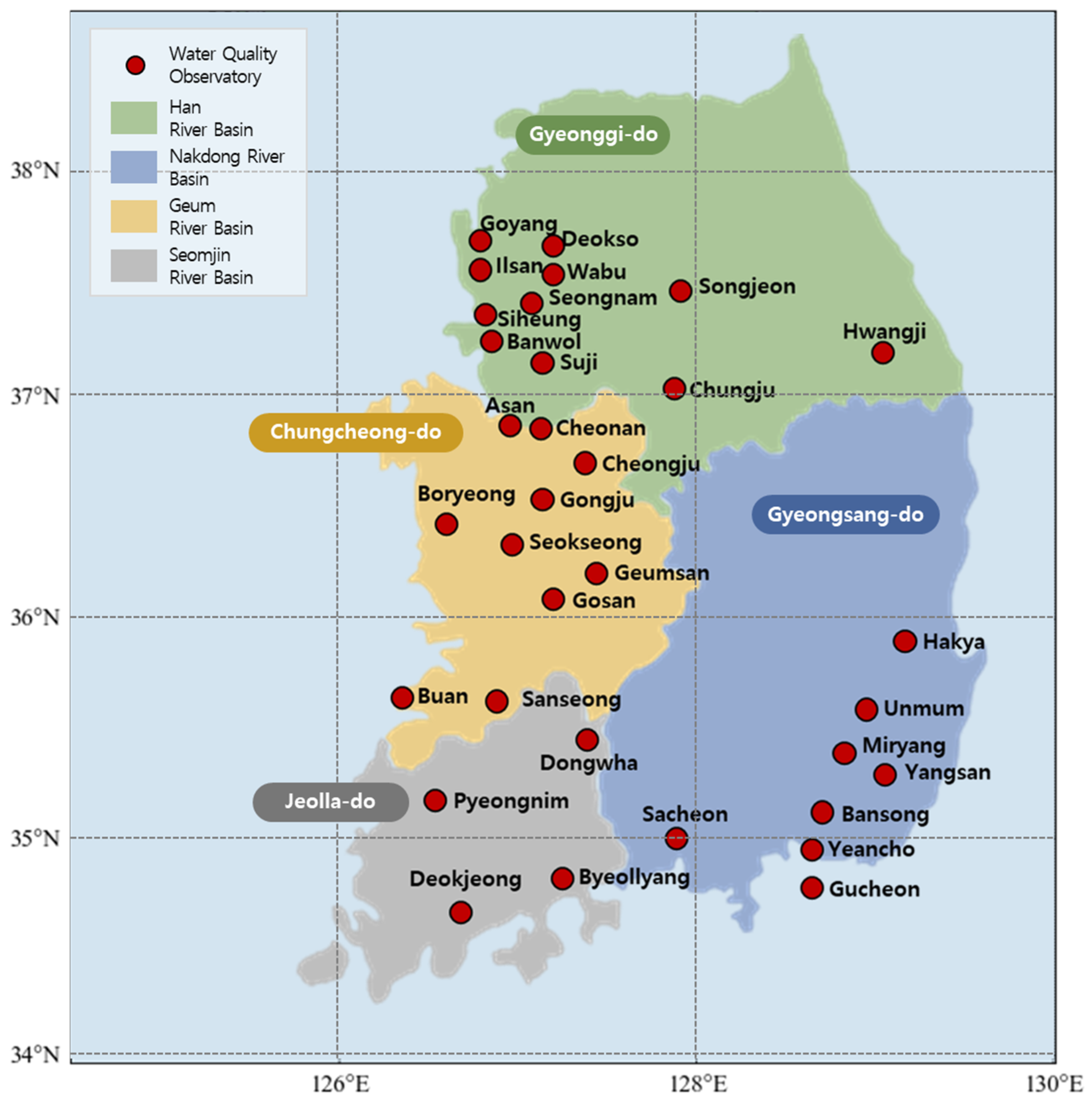
As shown in Figure 2, water management in South Korea is largely divided into four areas, and water supply facilities are operated based on the major basins in each area. The water supply facilities for the Han River basin, Geum River basin, Seomjin River and Yeongsan River basins, and Nakdong River basin are located in the Gyeonggi, Chungcheong, Jeolla, and Gyeongsang provinces, respectively [6]. On this basis, we analyzed the tap water quality characteristics of large water purification plants serving the water systems of all five major rivers in South Korea. Figure 2 shows the basins of these five major rivers and the status of major water purification plant facilities in each basin. The Han River basin, located in the central region of the Korean Peninsula, is the largest river basin in South Korea, with 11 water purification plants, including Goyang and Deokso. The Nakdong River basin is in the southeastern region of South Korea and contains eight water purification plants, including Gucheon and Miryang. The Geum River basin is in the southern midwest region of the Korean Peninsula. It is the third-largest river after the Han River and Nakdong River and has ten water purification plants, including Gosan and Gongju. The Seomjin River and Yeongsan River basins, located in the southern midwest region of the Korean Peninsula, contain four water purification plants, including Deokjeong and Donghwa.

3.3. Temporal Range

The study period of five-and-a-half years from January 2017 to May 2022 was selected to reveal the seasonal and long-term variation characteristics of the water quality environment. From this dataset, five years of data (1 January 2017 to 31 December 2021) were used for the exploratory data analysis and model training, and data from the remaining five months (1 January 2022 to 31 May 2022) was used for model validation (

Table 2. Composition of the dataset.

Dataset	Period	Observed Data
Modeling (training)	1 January 2017–31 December 2021	4,338,576
Model validation (out of sample)	1 January 2022–31 May 2022	358,776

). First, we performed exploratory data analysis on pH, turbidity, and residual chloride data to train the model, then identified the characteristics of the water quality data to develop a water quality prediction model. To prevent overfitting, we applied a time series cross-validation method to five months of data (January to May 2022) to verify the performance of the developed model.

3.4. Data Preprocessing

The datasets used in this study consisted of water quality data samples from 33 water purification plants. Each dataset contained 47,448 h of data for three indicators of tap water quality: pH, turbidity, and residual chloride. Generally, data preprocessing methods such as linear interpolation, smoothing, filtering, and noise removal can be applied to correct for missing data. Considering that the data were a time series, we linearly interpolated the water quality data as an hourly record. Regarding missing values judged to be sensor errors in the water quality data (0 or −999), we found 7989, 7352, and 7449 missing values for pH, turbidity, and residual chloride in 11 water purification plants of the Han River basin; 8402, 8359, and 8174 missing values in 10 water purification plants of the Geum River basin; 1938, 1542, and 1513 missing values in eight water purification plants of the Nakdong River basin; and 503, 586, and 489 missing values in four water purification plants of the Seomjin River basin, respectively. These missing values are expected to cause sensor failure because they frequently and continuously occur; as the longest period of delayed response was 305 h (approximately 12 days), the emergency response system of the management and supervision agency was considered to be inadequate.

4. Exploratory Data Analysis

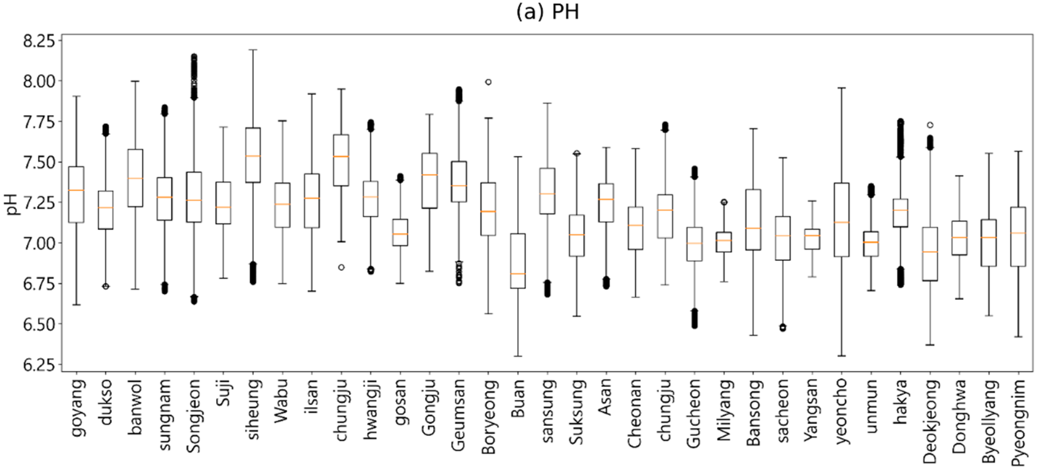
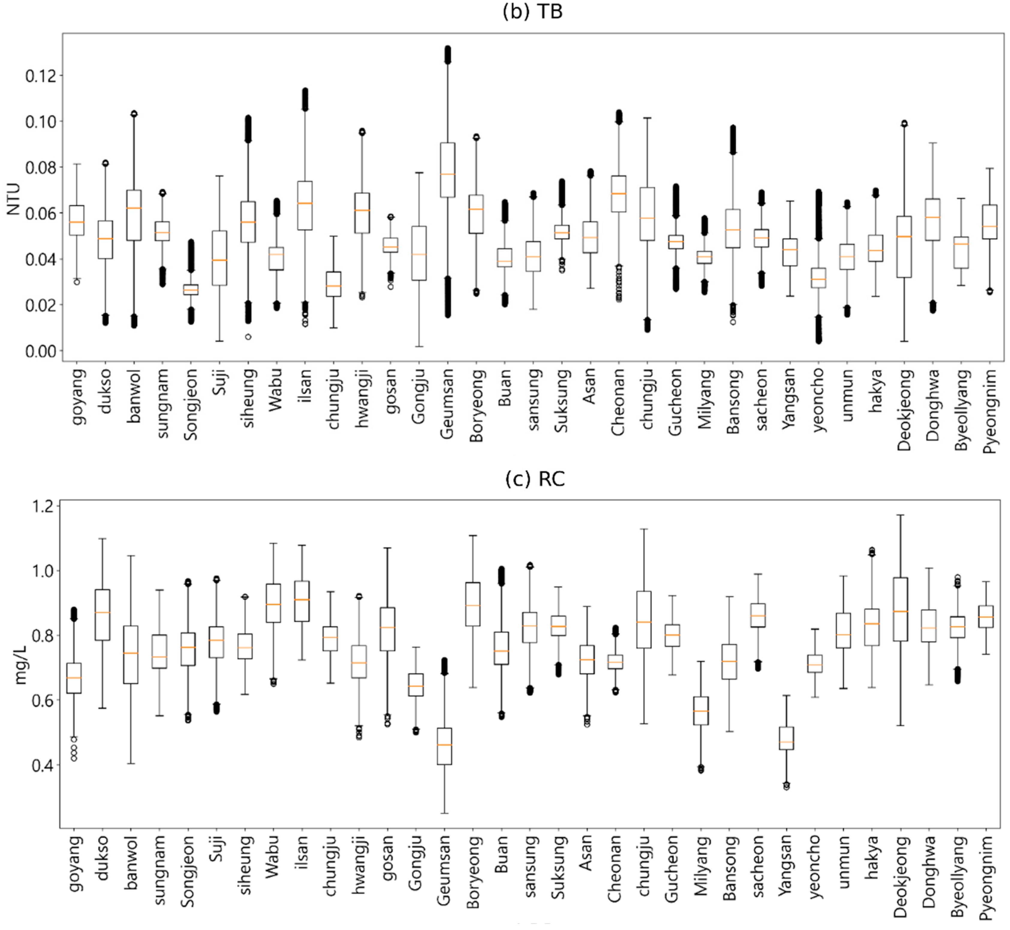
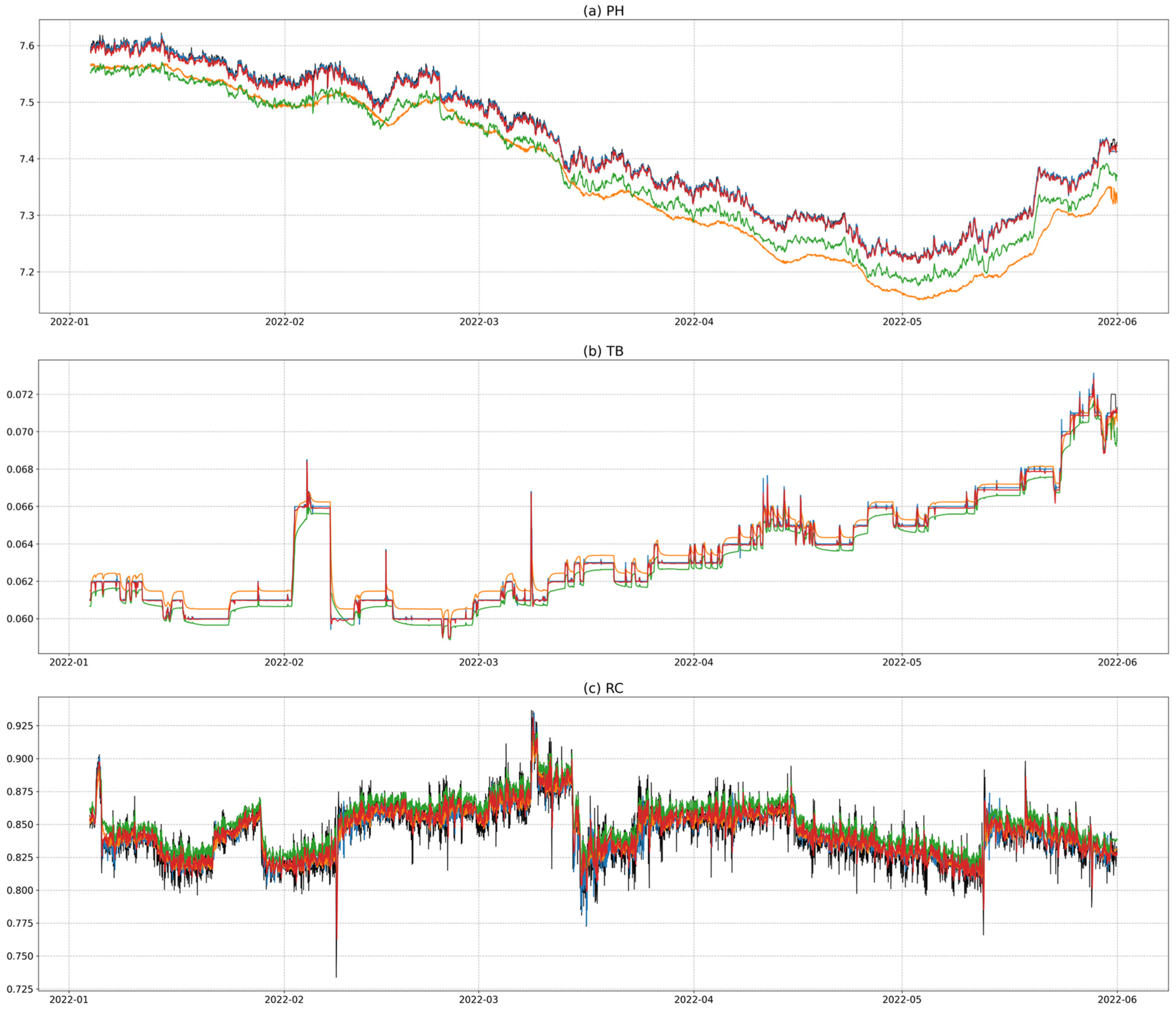
After preprocessing the water quality data according to Korean drinking water quality standards, we conducted the exploratory data analysis [27]. We performed exploratory data analysis on hourly observations of pH (PH), turbidity (TB), and residual chloride (RC) using five years of data from 2017 to 2021. First, we identified the water quality characteristics using various visualization methods based on the observational data, and then examined correlations between the water quality indicators through correlation analysis. Next, we investigated whether the tap water met the drinking water quality standards of the Ministry of Environment. Figure 3 shows the change patterns of each variable.

4.1. Correlation Analysis

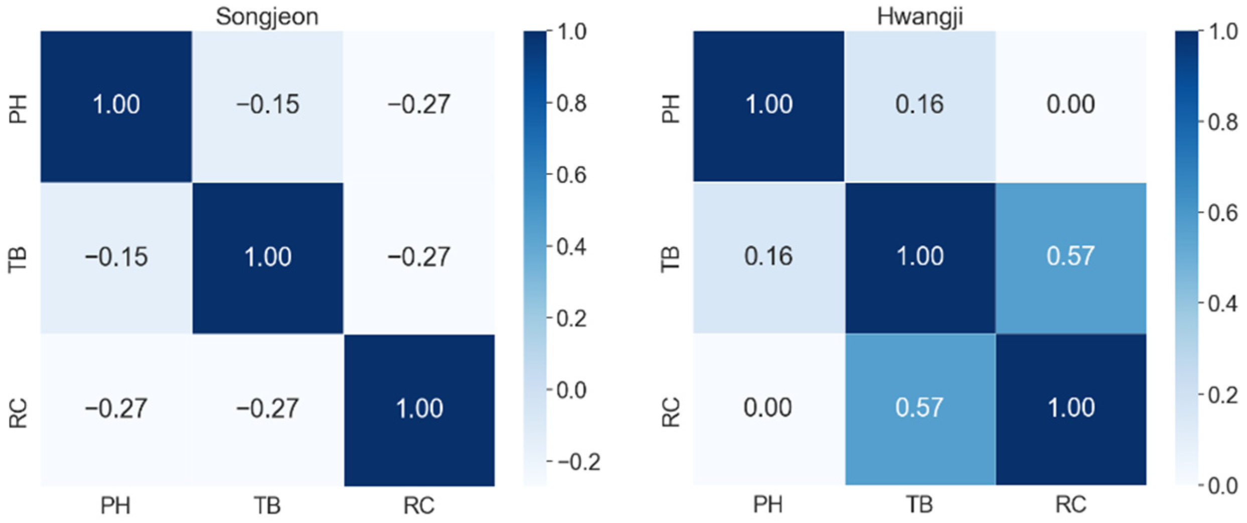
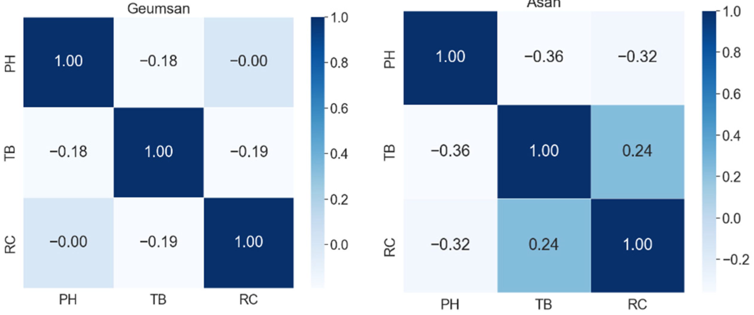
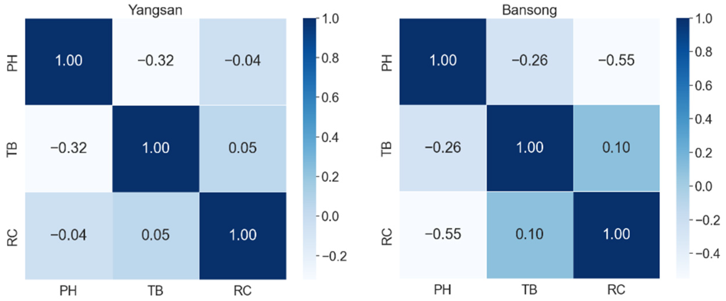
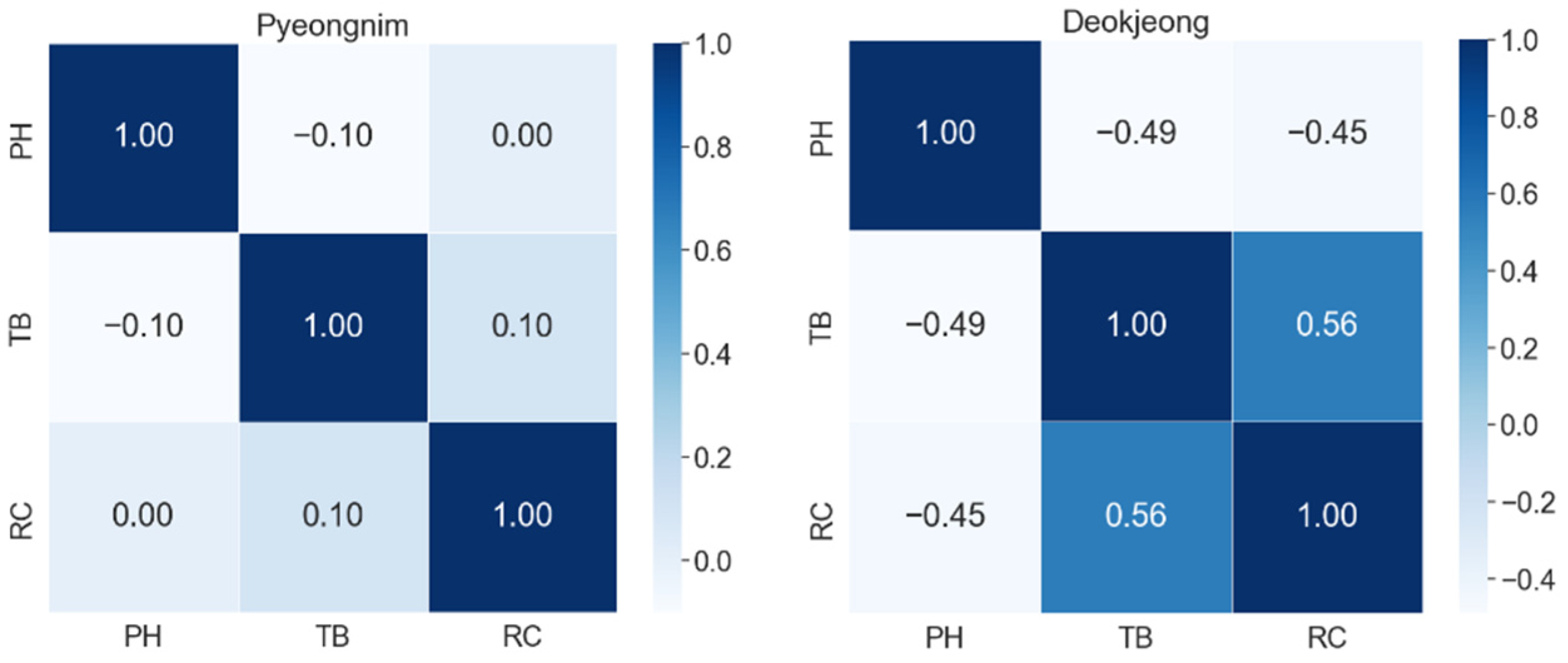
For multivariate correlation analysis of water quality information, it was essential to analyze and select correlations between various indicators [7]. In this study, we analyzed the relationships between three water quality indicators of large water purification plants in South Korea using Spearman correlation coefficients. The magnitude of the correlation coefficient indicates the degree of correlation and the sign indicates the direction of the correlation. Figure 4, Figure 5, Figure 6 and Figure 7 show the water purification plants with the highest and lowest correlations for each river basin.

The relationships between the three water quality indicators (variables) had a correlation coefficient of 0.6 or less in all four basins, indicating a low correlation. Although the correlation coefficients differed by basin, most water purification plants showed low correlation coefficients. Thus, when using Korean tap water quality datasets to create a water quality prediction model, a univariate model was more appropriate than a multivariate model.

4.2. Anomaly Analysis

To understand the characteristics of the drinking water quality data, we analyzed water quality anomaly data that did not meet the drinking water quality standards according to water quality indicators. The average water quality values of most tap water samples were within the acceptable range of the Ministry of Environment’s drinking water guidelines. However, some water quality measurements were outside the acceptable range, with 702 tap water quality anomalies occurring over the past five years. Therefore, we analyzed the water quality anomalies for each water quality indicator. pH had the most anomalies (460), followed by turbidity (236), whereas residual chloride had far fewer anomalies (6).

Next, we searched for anomalies in the five years of drinking water quality data for each basin (Figure 8). The Han River basin had 48 pH anomalies and 66 turbidity anomalies, 45 of which occurred at the Wabu water purification plant, where 43 exceeded the drinking water standard over three days from 14 to 16 December 2019. Outside the Wabu water purification plant, the Han River basin consistently had 15 or fewer pH and turbidity anomalies per year, indicating relatively stable water quality. No measurements exceeded the drinking water standards for residual chloride in the Han River basin. The Geum River basin had 80 pH anomalies, 42 turbidity anomalies, and 4 residual chloride anomalies; 37 of the pH anomalies occurred at the Buan water purification plant, with 25 occurring continuously over two days from 5 to 6 October 2020. The Nakdong River basin had 302 pH anomalies, 108 turbidity anomalies, and no residual chloride anomalies. The proportion of pH anomalies in the Nakdong River basin was higher than that in the other basins; of the 302 anomalies, 252 occurred in the Yeoncho water purification plant, 197 of which occurred over 12 days from 18 to 29 October 2020. Finally, the Seomjin River basin had 30 pH anomalies, 19 turbidity anomalies, and no residual chloride anomalies; 19 of the pH anomalies occurred at the Dongwha water purification plant, 16 of which occurred over a continuous period. All water quality anomalies occurred for at least two consecutive days in each basin, indicating a lack of swift responses to anomalies in tap water quality.

Figure 8 indicates frequency measurements of exceeding the drinking water standards; however, less than 0.01% of all measurements exceeded the standards over all five years. Based on our analysis of the water quality characteristics, we attribute the rather small number of anomalies in the study period to the fact that tap water quality data in South Korea are provided as hourly averages and one-time measurements; therefore, it is difficult to provide information on water quality anomalies that prompted a response in less than an hour. There are no standards for disclosing tap water quality information, which highlights the need to construct a system to monitor water quality in real time.

5. Development of Tap Water Quality Prediction Models

5.1. Deep Learning-Based Methods

5.1.1. LSTM

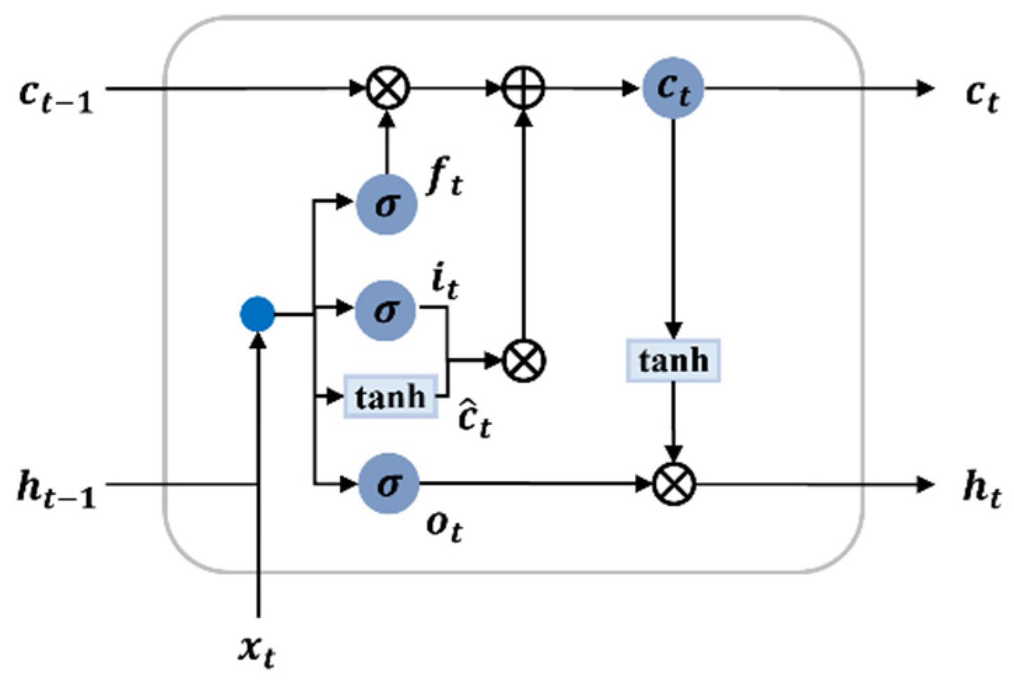
The LSTM method [9], which was proposed to solve the problems of RNNs, replaces the internal nodes with a device called a memory cell and uses a switchgear designed to accumulate information over long periods of time or forget previous information. Figure 9 shows the basic structure of the LSTM cell. The inside of each LSTM block comprises a memory cell, input gate, forget gate, and output gate, which can control information transfer in the hidden layer cell state [28]. The input gate returns information to the storage cell, the forget gate allows cell information to be forgotten or removed in the input storage cell, and the output gate outputs information from the input storage cell [29].

5.1.2. GRU

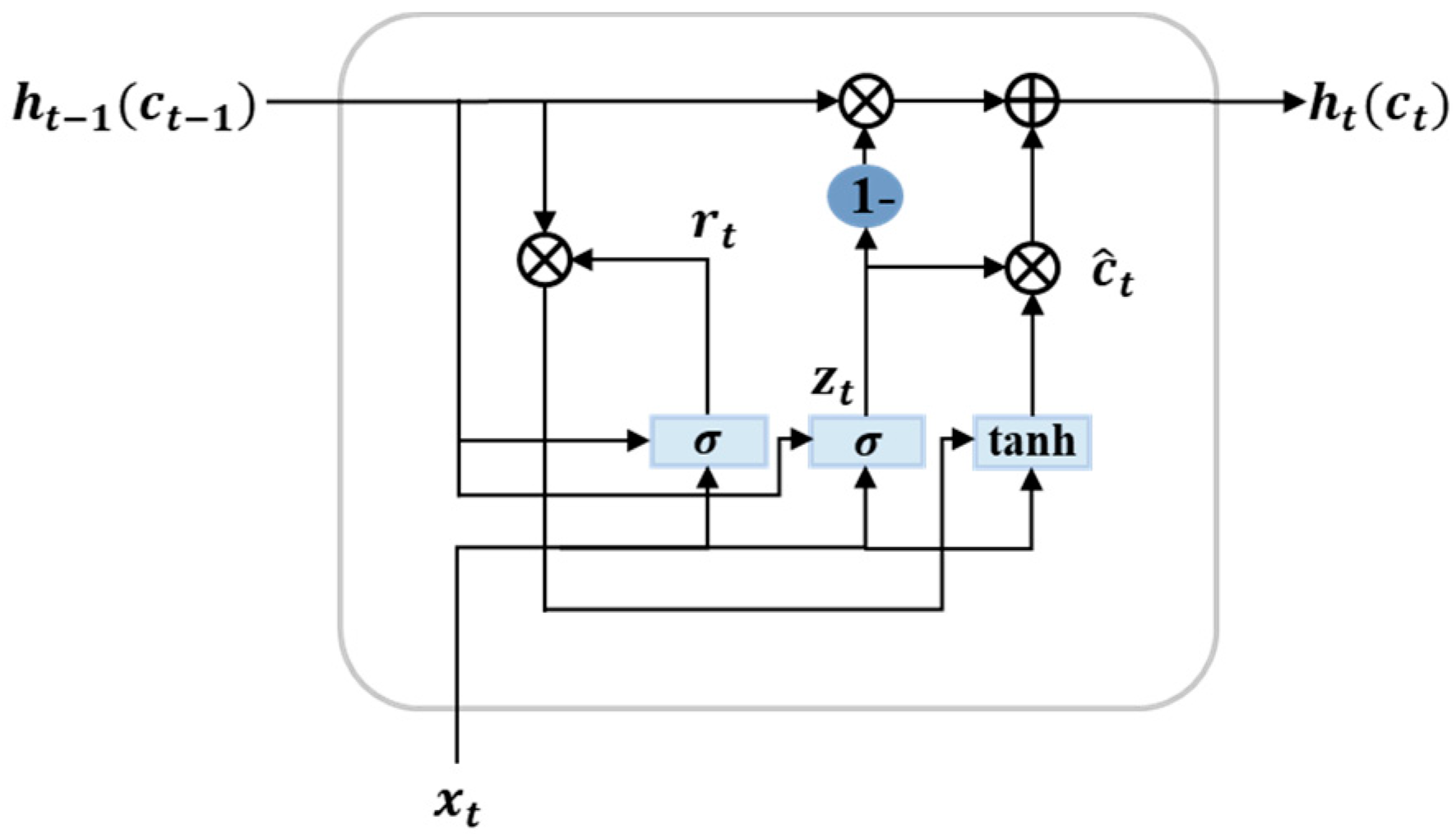
Due to its complex structure, the training process required to develop an LSTM neural network is typically very time-consuming. To speed up this process, a GRU network that is similar to the LSTM network but modified to have a simpler structure has been proposed [10]. Figure 10 shows the general structure of the GRU cell, which consists of two gates: update gate (${\mathrm{z}}_{\mathrm{t}}$) and reset gate (${\mathrm{r}}_{\mathrm{t}}$). Similar to LSTM cells, the hidden state output at time t is computed using the hidden state at time t-1 and the input time series value at time t. The update gate ${\mathrm{z}}_{\mathrm{t}}$ is used to control the degree to which the previous hidden state enters the current input state. The reset gate ${\mathrm{r}}_{\mathrm{t}}$ is used to determine the amount of previous information that is discarded. ${\mathrm{z}}_{\mathrm{t}}$ is the output of the update gate at time t, ${\mathrm{r}}_{\mathrm{t}}$ is the value of the reset gate at time t, $\mathsf{\sigma }$ is the sigmoid activation function, and ${\mathrm{h}}_{\mathrm{t}-1}$ is the hidden state at $\mathrm{t}-1$. ${\mathrm{x}}_{\mathrm{t}}$ is the input vector of the current time. ${\mathrm{W}}_{\mathrm{rx}}$, ${\mathrm{W}}_{\mathrm{rh}}$, and ${\mathrm{b}}_{\mathrm{r}}$ are the corresponding weight matrix and bias vectors. The reset gate output at the current time ${\mathrm{r}}_{\mathrm{t}}$ is bit multiplied by the hidden state at the previous time ${\mathrm{h}}_{\mathrm{t}-1}$. The candidate hidden state is calculated using the result of the operation and the input of the current time. A related operation is performed through the update gate to obtain the hidden state ${\mathrm{h}}_{\mathrm{t}-1}$ of the last moment and the current candidate hidden state ${\mathrm{h}}_{\mathrm{t}}$. The GRU neural network is a time-recursive neural network; therefore, the gate-loop unit can hold relevant information and pass it on to the next unit that fully reflects the long-term historical course of the time series and is thus suitable for the long-term prediction of time series.

5.1.3. SCINet

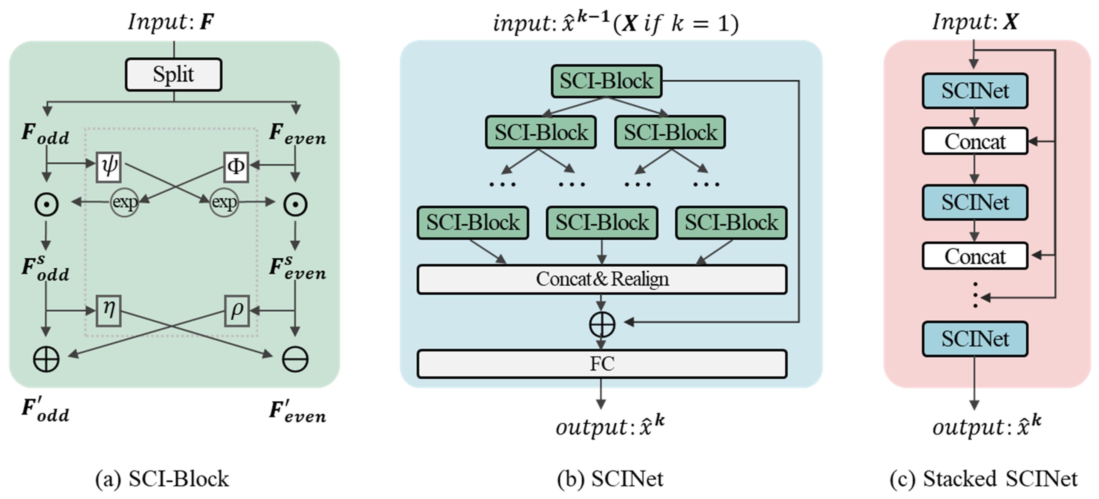
SCINet, proposed by [11], is a binary tree-based deep learning model comprising three levels: SCI-block, SCINet, and stacked SCINet, which captures time dependencies at multiple temporal resolutions to increase the predictability of the original time series. The basic block, SCI-block, decomposes the input data into even and odd sequences. It then processes using different convolution filters to extract homogeneous and heterogeneous information from each part. SCINet arranges the SCI-blocks in a binary tree structure then rearranges the child series. It concatenates all low-resolution elements into a new sequence representation, then adds them to the original time series for prediction. A stacked SCINet is composed of several SCINets with intermediate supervision. SCI-block uses different convolution kernels to extract information from two sequences. It is then used to compensate for information loss, which comprises two steps of interactive learning. The stacked SCINet architecture is shown in Figure 11a. SCINet comprises several SCI-blocks hierarchically arranged using the presented SCI-blocks to obtain the tree structure framework shown in Figure 11b. If the training sample is sufficient, then K SCINet layers can be stacked to achieve better prediction accuracy at the expense of a more complex model architecture, as shown in Figure 11c.

5.2. Classical Statistical Methods

Based on the ARMA model, the ARIMA model includes an additional process of normalizing nonstationary data that satisfies the assumption of stationarity. A normalized time series looks the same at any time point regardless of when it is observed. The three parameters that describe the three main components of the ARIMA model are p, d, and q. Several methods exist for converting a nonstationary time series into a stationary time series; one method involves generating d through differencing. Through the AR model order p, which indicates how many past values must be considered for prediction, and the MA model order q, which considers past prediction errors, the ARIMA model can be generalized to the ARIMA(p,d,q) model. Time series analysis consists of model identification, model estimation, and model testing steps, and it is important to configure a model suitable for each time series data.

In the AR model (Equation (1)), the variable of interest is predicted using the variable’s past values and the AR model is used only for data that shows stationarity. The MA model (Equation (2)) uses past prediction errors in a model similar to a regression model to express the weighted moving average of past prediction errors.

$${\mathrm{y}}_{\mathrm{t}}=\mathrm{c}+{\varnothing }_1{\mathrm{y}}_{\mathrm{t}-1}+{\varnothing }_2{\mathrm{y}}_{\mathrm{t}-2}+\dots +{\varnothing }_{\mathrm{p}}{\mathrm{y}}_{\mathrm{t}-\mathrm{p}}+{\mathsf{\epsilon }}_{\mathrm{t}}$$

(1)

$${\mathrm{y}}_{\mathrm{t}}=\mathrm{c}+{\mathsf{\epsilon }}_{\mathrm{t}}+{\varnothing }_1{\mathsf{\epsilon }}_{\mathrm{t}-1}+{\varnothing }_2{\mathsf{\epsilon }}_{\mathrm{t}-2}+\dots +{\varnothing }_{\mathrm{q}}{\mathsf{\epsilon }}_{\mathrm{t}-\mathrm{q}}$$

(2)

ARIMA model identification determines the difference order d, AR order p, and MA order q, which are judged through an auto correlation function (ACF) and partial auto correlation function (PACF). After identifying the specific models of ARIMA(p,d,q), it is necessary to estimate the selected models and test which model is most suitable. Akaike’s information criterion (AIC), which estimates the quality of a statistical model, was used as the test method in this study (Equation (3)). The AIC is advantageous for comparing different estimated models, where models with a smaller value have higher quality. The established time series model can accurately predict and detect anomalies according to how well the temporal characteristics of specific data are included; thus, it is necessary to identify and test the most suitable prediction model.

$$\mathrm{AIC}=-2\log \left(\mathrm{L}\right)+2\left(\mathrm{p}+\mathrm{q}+\mathrm{k}+1\right)$$

(3)

5.3. Tap Water Quality Prediction Models

In this section, we introduce the statistical and deep learning models used, and describe how their parameters were tuned and selected. All methods described below were implemented in Python using the NumPy, Pandas, and Matplotlib libraries, as well as the Statsmodels, Scikit-learn, Keras, and PyTorch packages for the time series and deep learning methods. All the modelling, data analysis, and visualization were conducted in the environment of Python 3.8.

5.3.1. Architecture of LSTM, GRU, and SCINet Models

The LSTM and GRU model were built using Tensorflow, which is an end-to-end machine learning platform in Python. The TensorFlow framework was selected because of its wide applications in industrial deployment and was used in the study along with Keras. It is helpful for various applications but is notably well-suited for the training and inference of deep neural networks. The LSTM and GRU were actualized with the Keras 2.9.0, TensorFlow version 2.9.1, CUDA version 11.2, and NumPy 1.18.1 libraries. The other libraries used in this study included Numpy version 1.23.1, Matplotlib version 3.5.3, Pandas version 1.4.3, and Scikit-learn version 1.1.1. The SCINet was implemented with PyTorch (https://github.com/cure-lab/SCINet, accessed on 22 August 2022). Deep learning models were trained using Python 3.8 in the following environment: Ubuntu 18.04.6 LTS OS, Intel(R) Xeon(R) Silver 4214R 2.40 GHz CPU, NVIDIA GeForce RTX 3090 (24 GB RAM) GPU, 512 GB RAM.

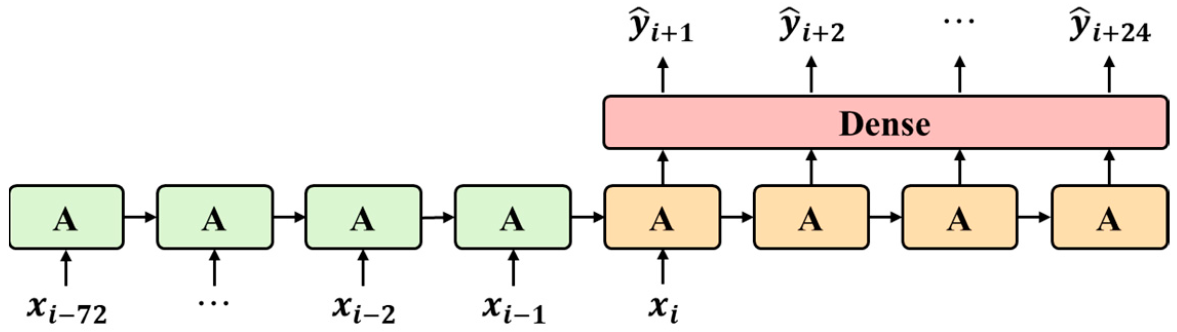
For a fair comparison of the three deep learning models, we maintained all input lengths and used multiple output strategies for multi-step prediction. First, because of the network similarity of LSTM and GRU, the same network architecture was designed for both models (Figure 12), with several network architectures tested using Bayesian optimization. According to the results, water quality predictions in the study area using LSTM and GRU networks containing only one layer were superior to those obtained using multi-layer networks. The proposed LSTM and GRU networks comprised one LSTM and GRU layer and one dense layer. Each LSTM and GRU layer consisted of 128 nodes and a linear function was used for the activation function of the dense layer. For the loss function, the mean squared error was used and the SCINet architecture proposed in Liu, Zeng, Xu, Lai, and Xu [11] was employed. The parameters used for univariate prediction were set as hidden size = 8, stacks = 1, levels = 3, and learning rate = 0.007.

Table 3. Hyperparameters in the Han, Geum, Nakdong, and Seomjin River datasets.

Model Configuration		Han River			Geum River			Nakdong River			Seomjin River
		PH	TB	RC	PH	TB	RC	PH	TB	RC	PH	TB	RC
LSTM	Other parameter	Input node: 128; activation: ReLU; dropout rate: 0.2; loss: mean squared error; optimizer: Adam; learning rate: 0.001; epoch: 200
	Batch size	34	24	39	58	47	32	34	47	39	34	36	39
GRU	Other parameter	Input node: 128; activation: ReLU; dropout rate: 0.2; loss: mean squared error; optimizer: Adam; learning rate: 0.001; epoch: 200
	Batch size	21	56	37	21	56	55	21	39	37	21	39	53
SCINet	Other parameter	Hidden size: 8; stacks: 1; levels: 3; learning rate: 0.007; batch size: 64; dropout: 0.25

presents the best hyperparameters values of three models.

5.3.2. Performance Comparison with the ARIMA Model

Time series analysis techniques are largely divided into univariate and multivariate techniques. The univariate technique assumes that time-dependent variables can be explained only with past data. In the previous correlation analysis, we confirmed that there was no correlation between pH, turbidity, and residual chloride, suggesting that the tap water quality data considered only time variables in the time series analysis. Given that the goal of this study was the temporal prediction of time series data, the univariate technique was considered preferable to the multivariate technique. Thus, we adopted the ARIMA model, which is a widely used univariate technique. Pandas version 1.3.4 and statsmodels version 0.13.2 from the Python 3.8 software package were adopted. Pandas was used to clean data and statsmodels was used to test, determine order, and fit and predict ARIMA. The other libraries for visualization used in this study included matplotlib version 3.5.1 and seaborn version 0.11.2.

We conducted a time series analysis on the hourly data of Korean water purification plants and estimated the time series model using the statistical packages SAS and R. First, by analyzing water quality data over five years from 2017 to 2021 and calculating the ACF and PACF, we estimated the most suitable models. As the water quality data of the 33 large-area water purification plants was nonstationary time series data, we performed first differencing to satisfy the stationarity assumption in the time series analysis before estimating the models. The ARIMA(p,d,q) models were constructed by measuring the correlations between data, where p in AR and q in MA were determined using ACF and PACF.

Both ACF and PACF of the pH water quality indicator in the Goyang water purification plant (Han River basin) were cut off after, at lag 2; thus, ARIMA(2,1,2) was estimated as a tentative model. The PACF value of pH in the Yeoncho water purification plant (Nakdong River basin) approached 0 at a slow rate and was unstable; however, ACF sharply declined at lag 2 after the differencing, indicating the MA(1) process. As such, the ARIMA(0,1,2) model was introduced through the model identification step. In the Byeolryang water purification plant of the Seomjin River basin, ACF and PACF were cut off at lag 2 and lag 1, respectively; therefore, the ARIMA(1,1,2) model was assigned for this plant. Then, using the AIC evaluation criteria, we established a water quality prediction model for the 33 large water purification plants in South Korea according to the time series model identification step based on ACF and PACF values.

In the model diagnosis step, we conducted a residual analysis to examine the correlation among the residuals. First, the model of the water purification plant with the lowest AIC was selected and applied to the water purification plants for each basin. Then, to investigate whether the residuals of the model applied to each basin were white noise processes, we performed a Ljung–Box test [30]. For the Han River basin, the ARIMA(2,1,2) model of the Goyang water purification plant, which had the lowest AIC, was applied to all water purification plants in the basin and the model was diagnosed. The p-values of the chi-squared statistic for pH, turbidity, and residual chloride all had a significance level of 0.05 or above. Hence, the ACF of the residuals showed no significant correlation and the estimated basin model was considered suitable. Accordingly, by testing the suitability of models for each basin, we selected the final tap water quality prediction models for each basin, as shown in

Table 4. Optimal ARIMA model for each basin.

Location	pH	Turbidity	Residual Chloride
Han River	ARIMA(2,1,2)	ARIMA(1,1,2)	ARIMA(2,1,1)
Geum River	ARIMA(1,1,3)	ARIMA(1,1,1)	ARIMA(1,1,3)
Nakdong River	ARIMA(0,1,2)	ARIMA(2,1,4)	ARIMA(1,1,2)
Seomjin River	ARIMA(0,1,2)	ARIMA(2,1,1)	ARIMA(1,1,2)

.

6. Model Performance Evaluation

6.1. Evaluation Method

In this study, we developed four prediction models (LSTM, GRU, SCINet, and ARIMA) and compared their prediction performance. To prevent overfitting, the last five months of data (1 January 2022, to 31 May 2022), which were not used for model training, were used to evaluate the prediction performance. Specifically, we simulated the behavior of the models for new data and applied several indicators and datasets to evaluate model performance in relation to pH, turbidity, and residual chloride prediction. To address the uncertainty of continuously changing water quality predictions, we combined actual tap water quality data sets from multiple regions nationwide, then trained the deep learning models based on approximately five years of data from January 2017 to December 2021. The prediction accuracy of the trained models was verified by repeating the water quality predictions over the next 24 h through the rolling forecasting method, which was performed on the last five months of the dataset.

6.2. Evaluation Metrics

The overall accuracy, MAE, RMSE, and NSE were used as evaluation metrics to assess the effectiveness of the proposed prediction models. MAE and RMSE are advantageous for comparing different estimating models, where smaller values indicate a more suitable model. A model is supposed to be ideal with optimized results if the NSE criterion on the estimated values is very close to 1 or the value of NSE is more than 0.8 [31]. In the following equations, ${\hat{\mathrm{y}}}_{\mathrm{i}}$ indicates the predicted value, ${\mathrm{y}}_{\mathrm{i}}$ indicates the actual value, $\overline{\mathrm{y}}$ is the mean value taken over n, and $\mathrm{n}$ is the number of predicted sample series.

$$\mathrm{Overall}\mathrm{Accuracy}(\%)=\frac{1}{\mathrm{n}}{\sum }_{\mathrm{i}=1}^{\mathrm{n}}\left(1-\frac{\left|{\mathrm{y}}_{\mathrm{i}}-{\hat{\mathrm{y}}}_{\mathrm{i}}\right|}{{\mathrm{y}}_{\mathrm{i}}}\right)$$

(4)

$$\mathrm{MAE}=\frac{1}{\mathrm{n}}{\sum }_{\mathrm{i}=1}^{\mathrm{n}}\left|{\mathrm{y}}_{\mathrm{i}}-{\hat{\mathrm{y}}}_{\mathrm{i}}\right|$$

(5)

$$\mathrm{RMSE}=\sqrt{\frac{{\sum }_{\mathrm{i}=1}^{\mathrm{n}}{\left({\mathrm{y}}_{\mathrm{i}}-{\hat{\mathrm{y}}}_{\mathrm{i}}\right)}^2}{\mathrm{n}}}$$

(6)

$$\mathrm{NSE}=1-\frac{{\sum }_{\mathrm{i}=1}^{\mathrm{n}}{\left({\mathrm{y}}_{\mathrm{i}}-{\hat{\mathrm{y}}}_{\mathrm{i}}\right)}^2}{{\sum }_{\mathrm{i}=1}^{\mathrm{n}}{\left({\mathrm{y}}_{\mathrm{i}}-\overline{\mathrm{y}}\right)}^2}$$

(7)

6.3. Cross-Validation

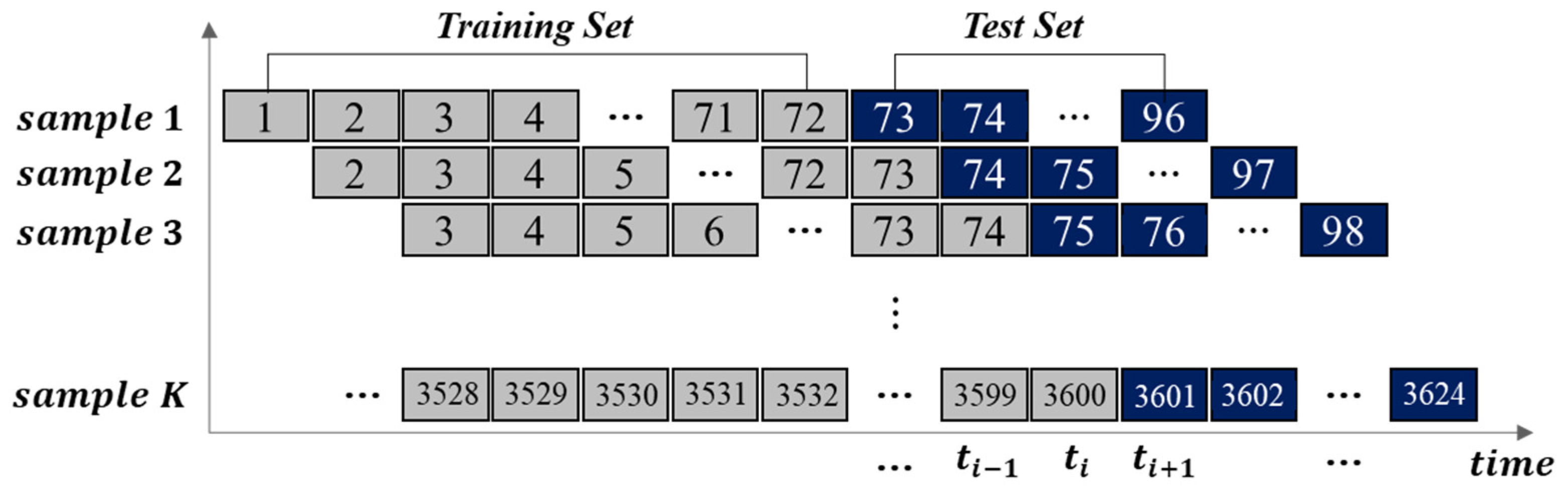
Regarding the experimental method, the first five years of data (January 2017 to December 2021) were used for the training set, and the remaining five months (1 January 2022, to 31 May 2022) were used for model validation. Time series cross-validation generally uses the rolling forecasting method to reconstruct time series data that has correlations between previous and subsequent data. Given a set of time series data, the previous time step is used as the input variable and the next time step is used as the output variable. To avoid overfitting, the rolling window method was used to cross-validate the performance of the model [32]. As shown in Figure 13, we used the fixed rolling window forecasting method, where the amount of data in each cross-validation was equally divided. This method fixed the size of the training and validation data sets in all cross-validation iterations to split the training and test data while preserving the chronologically arranged data.

Figure 14 shows the MAE values for the simulation results of the deep learning models with different time steps and prediction lead times. Each model was run three times for a given combination of time steps and prediction lead times. Through cross-validation, the optimal learning interval of the training set and test set was explored using the most recent 3624 water quality data points from January to May 2022. Considering that the water quality prediction period was one day, the training set size was reduced from 168 h (seven days) to increments of 24 h (one day) to verify the prediction performance. The results indicated that suitability was highest when the training set size was 72 h (three days). Accordingly, we selected 72 and 24 h for the training and test sets, respectively, and set each iteration to roll for 1 h.

6.4. Model Construction and Running Time

In the proposed models, we set the batch size (related to efficient resource usage in the deep learning models) to 20–64 and the epochs (related to the number of times the training data passes through the neural network) to 200. The Adam optimizer was used for optimization, which involves updating the actual parameters in the training process. Mean squared error (MSE), the most commonly used metric, was applied to measure the prediction error rate of the proposed models. Then, for each water quality indicator, we constructed the LSTM, GRU, and SCINet models and trained them to minimize errors by efficiently adjusting the hyperparameters using Bayesian optimization. The parameters used to train the networks are shown in

Table 5. Simulation of hyperparameters using Bayesian optimizer.

Parameters	LSTM	GRU	SCINet
Epochs	100	100	-
	200	200
Batch size = 64, optimizer = Adam, learning rate = 0.001
Accuracy (%) Time (min)	98.75	98.75	99.58
	98.71	98.73	99.55
	35	27	05
	27	25	05
Batch size = 128, optimizer = Adam, learning rate = 0.001
Accuracy (%) Time (min)	98.73	98.79	98.77
	98.72	98.76	98.89
	33	23	08
	24	20	07

, which also reveals that the LSTM and GRU models predicted water quality with nearly identical accuracy. Owing to the complex structure of LSTM neurons without the aid of a GPU, a training cycle with 100 iterations took approximately 30 min. In contrast, GRU had a simple structure and few parameters and took less time to train the model, thus may be the preferred method for short-term water quality predictions. SCINet had the shortest average training cycle at less than 10 min.

6.5. Overall Prediction Accuracy in Major River Basins

In this paper, the water quality prediction was conducted at the 33 large water purification plants of Korea, and the ARIMA model was selected as the baseline model for comparison with the deep learning models. The deep learning model parameters were determined based on trial and error. A comprehensive evaluation of the ARIMA, LSTM, GRU, and SCINet models and the best input scenarios to develop these models for 24 h prediction of water quality were considered for comparison.

Table 6. Overall accuracy evaluation of four model architectures.

Dataset	Indicator	pH				Turbidity				Residual Chloride
	Method	ARIMA	LSTM	GRU	SCINet	ARIMA	LSTM	GRU	SCINet	ARIMA	LSTM	GRU	SCINet
Han River
Goyang		0.99715	0.99281	0.99677	0.99719	0.98477	0.98042	0.98434	0.98719	0.98175	0.98174	0.98398	0.98592
Deokso		0.99735	0.99408	0.99487	0.99728	0.96943	0.96656	0.96879	0.97133	0.97699	0.98065	0.98131	0.98096
Banwol		0.98855	0.98508	0.98725	0.99021	0.97448	0.96857	0.97648	0.97183	0.88134	0.89947	0.91617	0.91870
Seongnam		0.99795	0.98195	0.99649	0.99795	0.90435	0.89575	0.90255	0.91811	0.97942	0.97722	0.98173	0.98351
Songjeon		0.99630	0.99501	0.99621	0.99658	0.93905	0.94128	0.92918	0.95416	0.95604	0.95201	0.84342	0.95865
Suji		0.99739	0.97795	0.97802	0.99748	0.90199	0.90542	0.90691	0.92447	0.94664	0.96040	0.96033	0.96149
Siheung		0.99712	0.98176	0.98499	0.99727	0.95739	0.90197	0.91485	0.96032	0.97480	0.95683	0.97566	0.98025
Wabu		0.99421	0.99378	0.99430	0.99501	0.94281	0.92375	0.93642	0.94623	0.97491	0.98067	0.97963	0.98131
Ilsan		0.99732	0.99161	0.99609	0.99717	0.97388	0.96456	0.97542	0.98011	0.97823	0.97697	0.97912	0.98051
Chungju		0.99231	0.98184	0.99282	0.99364	0.94169	0.93293	0.92548	0.95039	0.94928	0.95354	0.95295	0.95361
Hwangji		0.99660	0.99095	0.99424	0.99702	0.99336	0.96186	0.96387	0.98478	0.98226	0.96071	0.97667	0.98412
Geum River
Gosan		0.99752	0.98970	0.99637	0.99771	0.98707	0.96847	0.97202	0.98703	0.97598	0.98069	0.98072	0.98108
Gongju		0.99886	0.98308	0.99877	0.99894	0.97053	0.96019	0.96550	0.97792	0.97619	0.97714	0.97672	0.98282
Geumsan		0.99811	0.99553	0.99622	0.99809	0.98579	0.98648	0.98689	0.99071	0.96873	0.97041	0.97156	0.97236
Boryeong		0.99211	0.99040	0.99352	0.99591	0.96668	0.97149	0.97171	0.97644	0.97996	0.98066	0.98293	0.98338
Buan		0.99720	0.99646	0.99663	0.99693	0.91718	0.87630	0.86198	0.93233	0.96897	0.98066	0.97166	0.97172
Sanseong		0.99481	0.99389	0.99558	0.99581	0.94637	0.94994	0.95021	0.95995	0.95793	0.95959	0.95926	0.96423
Seokseong		0.98705	0.98603	0.98459	0.99352	0.95065	0.95701	0.95791	0.97192	0.94903	0.95834	0.95849	0.96211
Asan		0.99718	0.98874	0.99658	0.99838	0.96649	0.96965	0.97130	0.97317	0.97105	0.97485	0.97517	0.97603
Cheonan		0.99743	0.99676	0.99740	0.99851	0.98124	0.98108	0.98116	0.98317	0.98004	0.97380	0.97796	0.98036
Cheongju		0.99855	0.98836	0.99090	0.99797	0.90400	0.93815	0.93884	0.93990	0.91801	0.94180	0.94242	0.95701
Nakdong River
Gucheon		0.99538	0.99373	0.99362	0.99479	0.96746	0.97397	0.95964	0.98098	0.93704	0.94804	0.94934	0.95019
Miryang		0.99810	0.99443	0.99571	0.99810	0.96307	0.96014	0.96695	0.97329	0.97659	0.97299	0.97553	0.97674
Bansong		0.99788	0.99710	0.99469	0.99815	0.95958	0.95697	0.94961	0.95831	0.95668	0.95346	0.96087	0.95867
Sacheon		0.99497	0.99483	0.98901	0.99638	0.94955	0.94778	0.93498	0.96190	0.96047	0.96836	0.96693	0.97061
Yangsan		0.99707	0.99387	0.99123	0.99697	0.97905	0.95178	0.96784	0.98221	0.97156	0.97288	0.97249	0.97368
Yeoncho		0.99884	0.99774	0.99667	0.99876	0.89065	0.66796	0.66542	0.91065	0.97453	0.97500	0.97446	0.97658
Unmun		0.99754	0.99688	0.99441	0.99780	0.97116	0.97312	0.97816	0.98062	0.95991	0.96270	0.96112	0.96670
Hakya		0.99805	0.97437	0.99602	0.99769	0.95385	0.96060	0.95747	0.96079	0.95745	0.95546	0.96005	0.96117
Seomjin River
Deokjeong		0.99812	0.99071	0.99716	0.99792	0.97053	0.96247	0.97088	0.97457	0.96917	0.97497	0.97555	0.97590
Donghwa		0.99604	0.98659	0.99198	0.99614	0.99537	0.98720	0.99090	0.99476	0.98204	0.98277	0.98280	0.98437
Byeollyang		0.99886	0.99211	0.99878	0.99868	0.96725	0.97020	0.97592	0.97834	0.98765	0.98611	0.98749	0.98752
Pyeongnim		0.99720	0.99581	0.99261	0.99710	0.96929	0.97500	0.97294	0.98278	0.95703	0.95713	0.96111	0.96322

Note: Overall accuracy is reported as a percentage (%). The best results are shown in bold.

shows the overall accuracy of the rolling prediction results using the five-month test set of water purification plant data from the five major basins of South Korea. SCINet yielded superior prediction performance compared with the other models for all water quality variables. It was found that the prediction accuracy of the LSTM and GRU models was similar in predicting the three water quality indicators. The ARIMA model showed good prediction results for pH. This was likely because the pH water quality data were more stable than the other water quality variables; therefore, the trends could be more accurately predicted.

6.6. Long-Term Forecasting Results

When generating a prediction model, the data selected for input fields play a critical role in the model’s performance. In this study, we considered several best practices when selecting prediction variables and data types for the prediction performance analysis, before we measured the corresponding performance. We selected the top three best practices based on the three water quality variables in Table 6, as follows: for pH prediction, the datasets of the Yeoncho, Cheonan, and Byeolryang water purification plants; for turbidity prediction, those of the Donghwa, Geumsan, and Goyang water purification plants; and for residual chloride, those of the Byeolryang, Goyang, and Dongwha water purification plants. Finally, we compared the results of the various models using MAE, RMSE, and NSE based on the selected best practices (Yeoncho, Donghwa, and Byeolryang water purification plants for pH, turbidity, and residual chloride, respectively).

Table 7. Baseline comparisons under multi-step setting for best practices of time series forecasting tasks.

Methods	Metrics	pH			Turbidity			Residual Chloride
		Horizon			Horizon			Horizon
		6	12	24	6	12	24	6	12	24
ARIMA	MAE	0.0079	0.0095	0.0113	0.0004	0.0005	0.0008	0.0130	0.0137	0.0146
	RMSE	0.0060	0.0073	0.0086	0.0001	0.0002	0.0003	0.0095	0.0099	0.0104
	NSE	0.9957	0.9937	0.9909	0.9783	0.9612	0.9124	0.6236	0.5801	0.5276
LSTM	MAE	0.0490	0.0424	0.0469	0.0008	0.0008	0.0009	0.0113	0.0113	0.0117
	RMSE	0.0505	0.0445	0.0493	0.0009	0.0010	0.0011	0.0151	0.0152	0.0158
	NSE	0.6895	0.6203	0.6255	0.9549	0.9371	0.9076	0.6015	0.5731	0.5343
GRU	MAE	0.0272	0.0271	0.0329	0.0007	0.0007	0.0009	0.0099	0.0102	0.0107
	RMSE	0.0285	0.0288	0.0348	0.0008	0.0009	0.0011	0.0134	0.0139	0.0146
	NSE	0.8758	0.8731	0.8657	0.9443	0.9450	0.8808	0.5099	0.4604	0.4069
SCINet	MAE	0.0068	0.0077	0.0094	0.0002	0.0002	0.0003	0.0095	0.0099	0.0104
	RMSE	0.0087	0.0099	0.0122	0.0004	0.0005	0.0006	0.0130	0.0136	0.0144
	NSE	0.9948	0.9932	0.9894	0.9801	0.9679	0.9485	0.6254	0.5884	0.5394

shows the MAE, RMSE, and NSE values for the three water quality variables. All four models generally showed low values of MAE and RMSE. It can be said that all the developed ARIAM, LSTM, GRU, and SCINet models provided good water quality predictions. However, the SCINet model improved the baseline model for almost every water quality measure, and clearly outperformed the other two models. Compared with the baseline model, the SCINet model consistently improved the predictions for all water quality measures. On average, SCINet reduced the MAE by approximately 0.8% compared with LSTM and 0.4% compared with GRU. GRU showed slightly better performance than LSTM. In 84% of all time series, GRU outperformed LSTM. This shows that the GRU model was better than the LSTM model in capturing nonlinear information. A model is supposed to be ideal with optimized results if the NSE criterion of the estimated values is very close to 1 or the value of NSE is more than 0.8 [31]. For the prediction of pH, the NSE of ARIMA slightly outperformed the SCINet model, but both models showed very similar performance. In the case of the prediction of turbidity and residual chloride, the ARIMA model achieved the second best performance. Overall, the prediction accuracy of the model with a 6-h lead time was higher than that of the model with a 24-h lead time. Therefore, the SCINet model had higher prediction accuracy than the other models, indicating that the model could contribute to improving the short-term prediction accuracy of water quality in Korea, as well as more suitable for long-term water quality predictions in Korea.

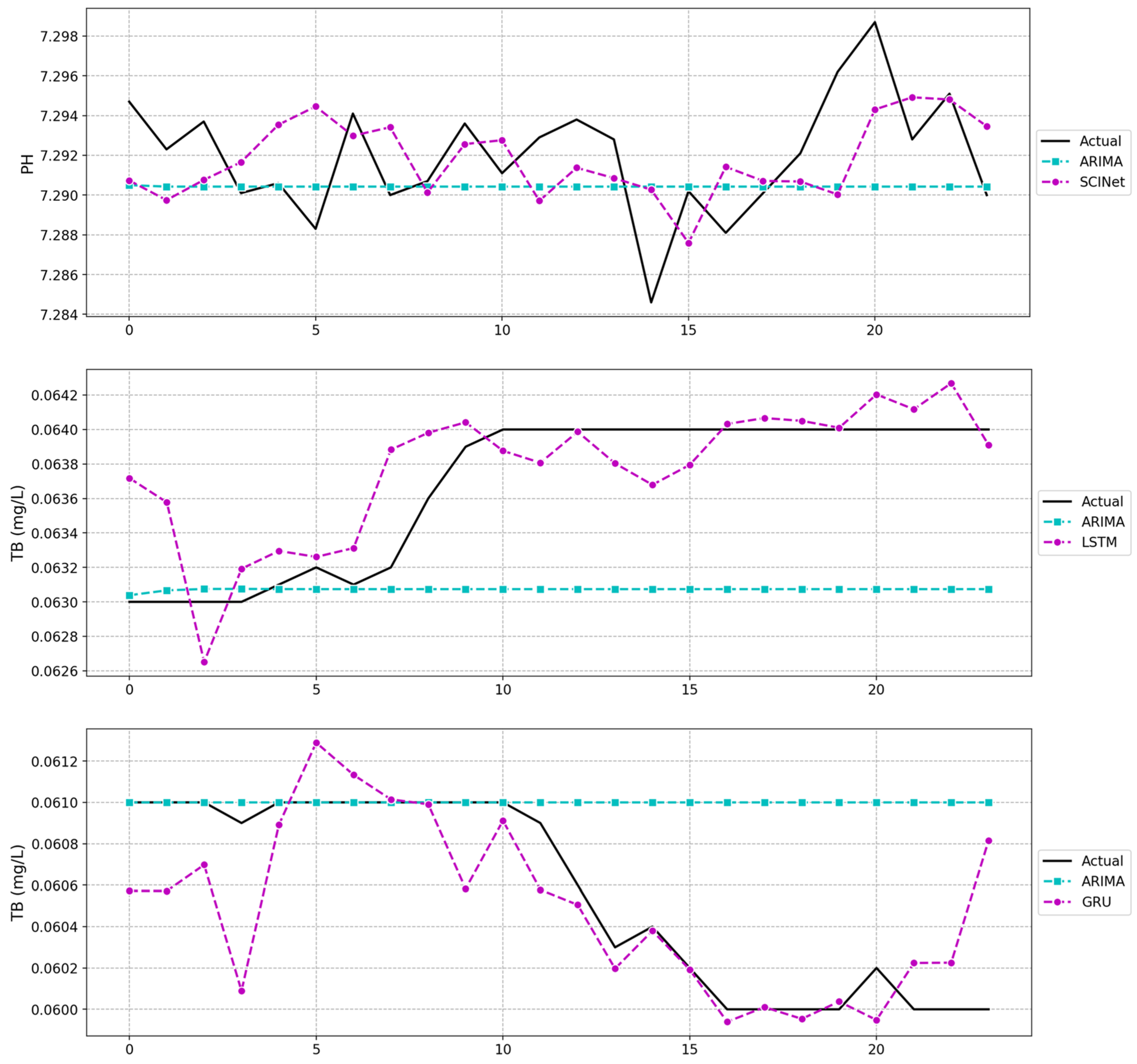
Based on the above results, the prediction results of pH, turbidity, and residual chloride using the best-practice models for each water quality variable are shown in Figure 15. The SCINet model performed better than the other alternatives in water quality prediction. Though this latest deep learning model showed consistently high accuracy in predicting pH, turbidity, and residual chloride values, it also provided significantly higher accuracy in predicting low and peak values. The SCINet model also showed robustness and reliable performance in predicting pH concentrations in different locations. However, the performance of the LSTM and GRU still had considerable variations at different locations (Figure 15a). ARIMA was suitable for analyzing time series data or predicting future data points on a time scale. However, ARIMA did not provide valid results when an increase or decrease trend was predicted (Figure 16). This is because ARIMA only considers time as a predictor variable, making it less effective for complex time series, such as predicting anomalies or pattern changes in water quality data containing abnormalities. The deep learning models showed better performance than the ARIMA in general, as well as in predicting a peak value. As such, it is difficult to apply the ARIMA model to the real-time monitoring environment as it cannot constantly predict changing water quality data. Creating real water quality simulation models is complex because they must consider the influence of physical, chemical, and biological factors and other external environments on water quality. Therefore, deep learning techniques, which can model complex environments and capture nonlinear regularities in water quality data, are more suitable than the ARIMA model for water quality anomaly detection systems.

7. Conclusions

In this study, we proposed a deep learning approach based on five-and-a-half years of actual water quality data collected from multiple water purification plants managed by K-water to enable real-time predictions of tap water quality on a national scale. Due to continuous anomalies in tap water quality, which is directly related to public health and safety, there is a high public distrust of tap water in South Korea. Therefore, a real-time monitoring system is important for promptly identifying continuously changing water quality conditions and pre-diagnosing hazards that could threaten tap water safety. To construct a real-time monitoring system, we divided the water systems in South Korea according to large basins, applied models, and predicted water quality. First, we conducted an in-depth data analysis of pH, turbidity, and residual chloride based on the water quality data of 33 large water purification plants. The results indicated that domestic tap water quality was generally stable, but that South Korea was lacking a clear response system in the event of sensor failure or water quality problems. Accordingly, we developed various deep learning models to predict the three monitoring indicators of drinking tap water quality based on the analysis data. Furthermore, to improve the prediction accuracy of the deep learning models, we used an optimization model that reduced training errors and enhanced model precision. We then verified the accuracy of the proposed method through a time series cross-validation using a five-month-long test set. According to MAE, RMSE, and NSE indicators, the SCINet model yielded the best performance. On average, SCINet reduced MAE by approximately 0.8% compared with LSTM and 0.4% compared with GRU. In summary, the optimal deep learning-based neural network model yielded excellent performance for water quality datasets from various sources. This model architecture can be used to successfully predict constantly changing water quality conditions, which is beneficial for monitoring and managing tap water quality. Moreover, our proposed deep learning-based architecture was highly efficient, effectively capturing time series patterns in the water quality prediction domain and demonstrating huge potential for long input sequences.

The potential of deep learning-based neural network models is fully revealed when trained on large datasets in which complex patterns can be detected. Unlike ARIMA, this approach does not depend on specific assumptions about the data, such as time series stationarity or the existence of data fields. However, these models are difficult to interpret and their behavior is difficult to intuit. Moreover, careful hyperparameter tuning is required to achieve effective results, as well as vast quantities of historical monitoring data to train LSTM- and GRU-based prediction models. Future research should consider deep learning models based on multivariate time series and seek to improve their prediction accuracy through optimization. For the LSTM and GRU models, as the temporal unit of the datasets was 1 h in this study, better performance would be expected when using high-quality data with a higher resolution. The proposed water quality prediction model could effectively contribute to the implementation of a safe tap water quality management plan in South Korea.

References

- National Waterworks Information System. Statistics of Waterworks 2020. Available online: https://www.waternow.go.kr/web/ssdoData?pMENUID=8 (accessed on 10 October 2022).
- Lee, C.W.; Lee, Y.J.; Park, J.S. Determination of the sensor placement for detection water quality problems in water supply systems. J. Korean Soc. Hazard Mitig. 2020, 20, 299–306. [Google Scholar] [CrossRef] [Green Version]
- Ryu, D.; Choi, T. Development of the Smart Device for Real Time Water Quality Monitoring. J. KIECS 2019, 14, 723–728. [Google Scholar] [CrossRef]
- Wang, J.; Zhang, L.; Zhang, W.; Wang, X. Reliable model of reservoir water quality prediction based on improved ARIMA method. Environ. Eng. Sci. 2019, 36, 1041–1048. [Google Scholar] [CrossRef]
- Desye, B.; Belete, B.; Asfaw Gebrezgi, Z.; Terefe Reda, T. Efficiency of treatment plant and drinking water quality assessment from source to household, gondar city, Northwest Ethiopia. J. Environ. Public Health 2021, 2021, 9974064. [Google Scholar] [CrossRef] [PubMed]
- Yi, S.; Ryu, M.; Suh, J.; Kim, S.; Seo, S.; Kim, S.; Jang, S. K-water’s integrated water resources management system (K-HIT, K-water Hydro Intelligent Toolkit). Water Int. 2020, 45, 552–573. [Google Scholar] [CrossRef]
- Zhou, J.; Wang, Y.; Xiao, F.; Wang, Y.; Sun, L. Water quality prediction method based on IGRA and LSTM. Water 2018, 10, 1148. [Google Scholar] [CrossRef] [Green Version]
- Dong, Q.; Lin, Y.; Bi, J.; Yuan, H. An integrated deep neural network approach for large-scale water quality time series prediction. In Proceedings of the 2019 IEEE International Conference on Systems, Man and Cybernetics (SMC), Bari, Italy, 6–9 October 2019; pp. 3537–3542. [Google Scholar]
- Hochreiter, S.; Schmidhuber, J. Long short-term memory. Neural Comput. 1997, 9, 1735–1780. [Google Scholar] [CrossRef]
- Cho, K.; Van Merriënboer, B.; Gulcehre, C.; Bahdanau, D.; Bougares, F.; Schwenk, H.; Bengio, Y. Learning phrase representations using RNN encoder-decoder for statistical machine translation. arXiv 2014, arXiv:1406.1078. [Google Scholar] [CrossRef]
- Liu, M.; Zeng, A.; Xu, Z.; Lai, Q.; Xu, Q. Time series is a special sequence: Forecasting with sample convolution and interaction. arXiv 2021, arXiv:2106.09305. [Google Scholar] [CrossRef]
- Ahmed, U.; Mumtaz, R.; Anwar, H.; Shah, A.A.; Irfan, R.; García-Nieto, J. Efficient water quality prediction using supervised machine learning. Water 2019, 11, 2210. [Google Scholar] [CrossRef]
- Chen, K.; Chen, H.; Zhou, C.; Huang, Y.; Qi, X.; Shen, R.; Liu, F.; Zuo, M.; Zou, X.; Wang, J. Comparative analysis of surface water quality prediction performance and identification of key water parameters using different machine learning models based on big data. Water Res. 2020, 171, 115454. [Google Scholar] [CrossRef] [PubMed]
- El Bilali, A.; Taleb, A. Prediction of irrigation water quality parameters using machine learning models in a semi-arid environment. J. Saudi Soc. Agric. Sci. 2020, 19, 439–451. [Google Scholar] [CrossRef]
- Loos, S.; Shin, C.M.; Sumihar, J.; Kim, K.; Cho, J.; Weerts, A.H. Ensemble data assimilation methods for improving river water quality forecasting accuracy. Water Res. 2020, 171, 115343. [Google Scholar] [CrossRef] [PubMed]
- Solanki, A.; Agrawal, H.; Khare, K. Predictive analysis of water quality parameters using deep learning. Int. J. Comput. Appl. 2015, 125, 0975–8887. [Google Scholar] [CrossRef] [Green Version]
- Singha, S.; Pasupuleti, S.; Singha, S.S.; Singh, R.; Kumar, S. Prediction of groundwater quality using efficient machine learning technique. Chemosphere 2021, 276, 130265. [Google Scholar] [CrossRef]
- Zhang, Y.; Gao, X.; Smith, K.; Inial, G.; Liu, S.; Conil, L.B.; Pan, B. Integrating water quality and operation into prediction of water production in drinking water treatment plants by genetic algorithm enhanced artificial neural network. Water Res. 2019, 164, 114888. [Google Scholar] [CrossRef] [PubMed]
- Liu, P.; Wang, J.; Sangaiah, A.K.; Xie, Y.; Yin, X. Analysis and prediction of water quality using LSTM deep neural networks in IoT environment. Sustainability 2019, 11, 2058. [Google Scholar] [CrossRef] [Green Version]
- Vadiati, M.; Rajabi Yami, Z.; Eskandari, E.; Nakhaei, M.; Kisi, O. Application of artificial intelligence models for prediction of groundwater level fluctuations: Case study (Tehran-Karaj alluvial aquifer). Environ. Monit. Assess. 2022, 194, 619. [Google Scholar] [CrossRef]
- Samani, S.; Vadiati, M.; Azizi, F.; Zamani, E.; Kisi, O. Groundwater Level Simulation Using Soft Computing Methods with Emphasis on Major Meteorological Components. Water Resour. Manag. 2022, 36, 3627–3647. [Google Scholar] [CrossRef]
- Peng, L.; Wu, H.; Gao, M.; Yi, H.; Xiong, Q.; Yang, L.; Cheng, S. TLT: Recurrent fine-tuning transfer learning for water quality long-term prediction. Water Res. 2022, 225, 119171. [Google Scholar] [CrossRef]
- Wu, J.; Zhang, J.; Tan, W.; Sheng, Y.; Zhang, S.; Meng, L.; Zou, X.; Lin, H.; Sun, G.; Guo, P. Prediction of the Total Phosphorus Index Based on ARIMA. In Proceedings of the International Conference on Artificial Intelligence and Security, Qinghai, China, 15–20 July 2022; pp. 333–347. [Google Scholar]
- Zhang, L.; Xin, F. Prediction model of river water quality time series based on ARIMA model. In Proceedings of the International Conference on Geo-Informatics in Sustainable Ecosystem and Society, Handan, China, 21–25 November 2018; pp. 127–133. [Google Scholar]
- Chen, Y.; Zheng, B. What happens after the rare earth crisis: A systematic literature review. Sustainability 2019, 11, 1288. [Google Scholar] [CrossRef] [Green Version]
- Abbas, F.; Feng, D.; Habib, S.; Rahman, U.; Rasool, A.; Yan, Z. Short term residential load forecasting: An improved optimal nonlinear auto regressive (NARX) method with exponential weight decay function. Electronics 2018, 7, 432. [Google Scholar] [CrossRef] [Green Version]
- Lee, J.H.; Song, G.W.; Im, Y.J.; Cho, M.S. Development of Predictive Time-Series Models for Anomaly Detection of Tap-Water Quality. KIISE Trans. Comput. Pract. 2022, 28, 465–473. [Google Scholar] [CrossRef]
- Fischer, T.; Krauss, C. Deep learning with long short-term memory networks for financial market predictions. Eur. J. Oper. Res. 2018, 270, 654–669. [Google Scholar] [CrossRef] [Green Version]
- Zhao, Z.; Chen, W.; Wu, X.; Chen, P.C.; Liu, J. LSTM network: A deep learning approach for short-term traffic forecast. IET Intell. Transp. Syst. 2017, 11, 68–75. [Google Scholar] [CrossRef] [Green Version]
- Box, G.E.; Jenkins, G.M.; Reinsel, G.C.; Ljung, G.M. Time Series Analysis: Forecasting and Control; John Wiley & Sons: Hoboken, NJ, USA, 2015. [Google Scholar]
- Moriasi, D.N.; Gitau, M.W.; Pai, N.; Daggupati, P. Hydrologic and water quality models: Performance measures and evaluation criteria. Trans. ASABE 2015, 58, 1763–1785. [Google Scholar] [CrossRef]
- Shojaei, A.; Flood, I. Univariate modeling of the timings and costs of unknown future project streams: A case study. Int. J. Adv. Syst. Meas. 2018, 11, 36–46. [Google Scholar]
Figure 1.
Proposed framework of the system.
Figure 2.
Map showing sampling stations in the basins of the Han, Geum, Nakdong, and Seomjin Rivers in the Korean Peninsula.
Figure 3.
Descriptive statistics of the water quality parameters analyzed in this study: (a) PH, (b) TB, and (c) RC.
Figure 4.
Spearman correlation coefficients for drinking water quality in the Han River basin.
Figure 5.
Spearman correlation coefficients for drinking water quality in the Geum River basin.
Figure 6.
Spearman correlation coefficients for drinking water quality in the Nakdong River basin.
Figure 7.
Spearman correlation coefficients for drinking water quality in the Seomjin River basin.
Figure 8.
Frequency of water quality anomalies in the Han, Geum, Nakdong, and Seomjin River basins.
Figure 9.
Overall architecture of LSTM network.
Figure 10.
Overall architecture of the GRU network.
Figure 11.
Overall architecture of SCINet (reproduced from ref. [11]).
Figure 12.
Multi-step architecture of LSTM and GRU models using the multi-output strategy.
Figure 13.
Visual representation of the cross-validation methods used for model evaluation based on a fixed window rolling forecast.
Figure 14.
MAE values of (a) PH, (b) TB, and (c) RC, predicted with different prediction lead times and time steps.
Figure 15.
Comparison of actual and predicted (a) PH, (b) TB, and (c) RC values for ARIMA, LSTM, GRU, and SCINet models.
Figure 16.
Comparison of actual and predicted water quality values for ARIMA and deep learning models over a 24-h period.