
Tidal Sediment Supply Maintains Marsh Accretion on the Yangtze Delta despite Rising Sea Levels and Falling Fluvial Sediment Input
Abstract
:1. Introduction
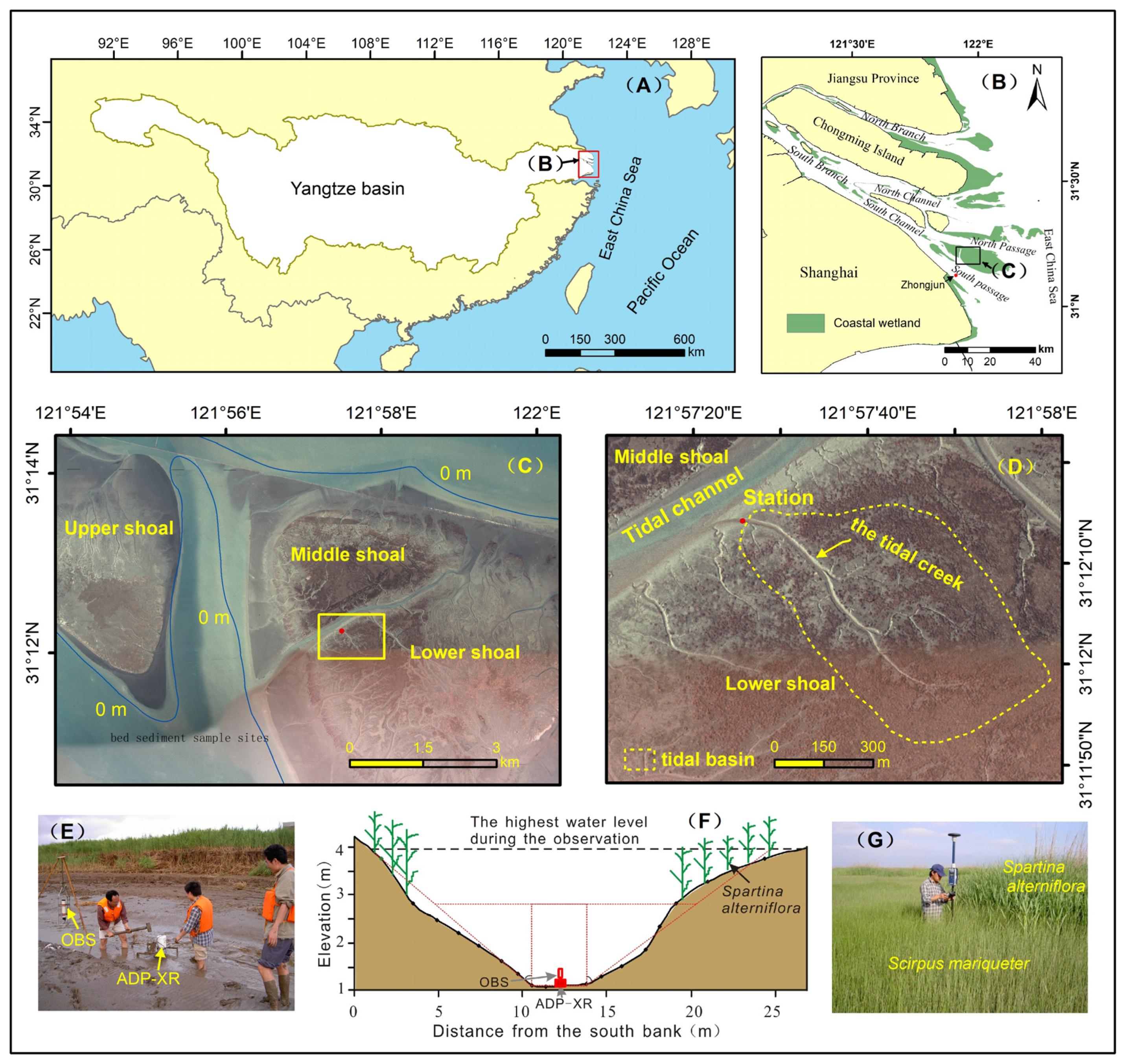
2. Field Setting
3. Materials and Methods
3.1. Field Measurement
3.2. Calibration of SSC and Sediment Transportation
3.3. Tidal Basin Area
4. Results
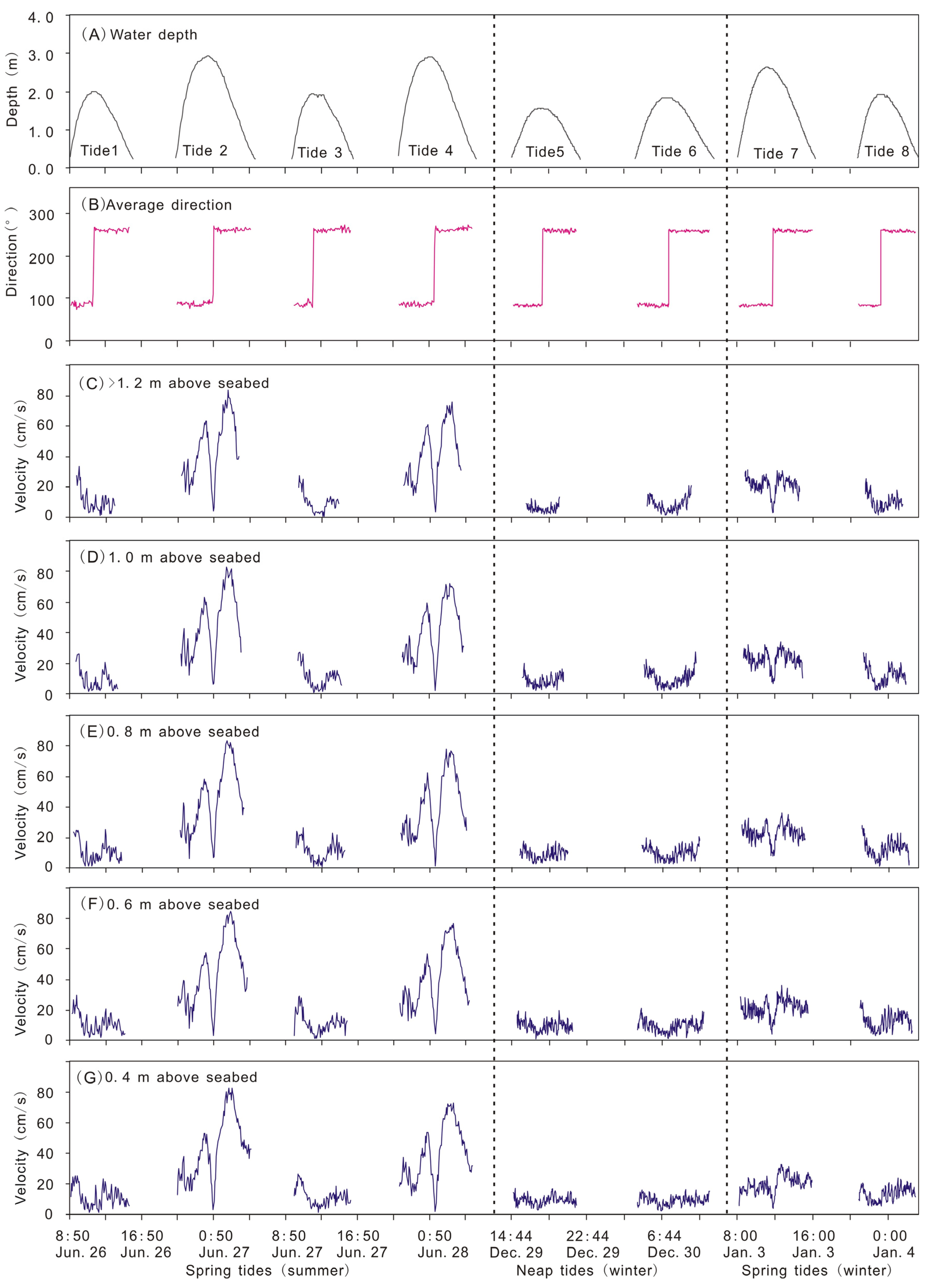
4.1. Tidal Current
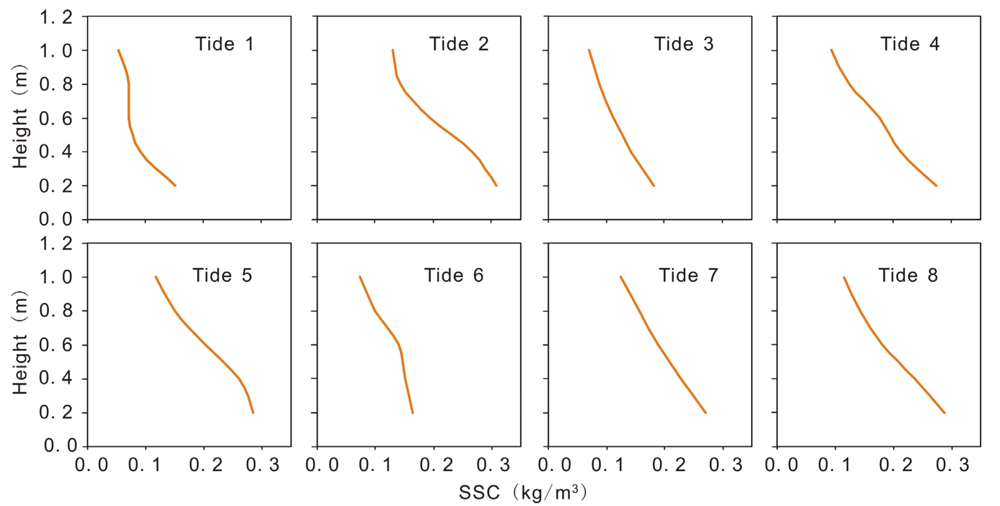
4.2. SSC Variations
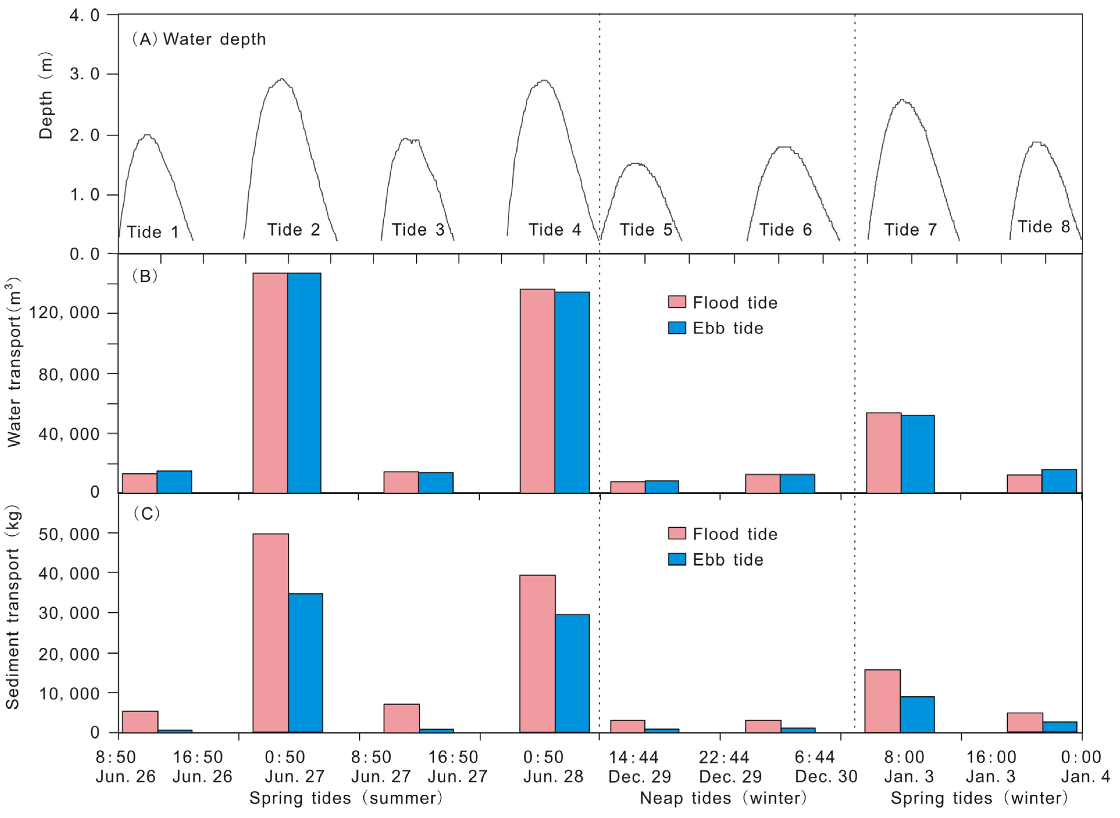
4.3. Sediment Transport in the Tidal Creek
4.4. Accretion Rate in the Tidal Basin
5. Discussion
6. Conclusions
Author Contributions
Funding
Institutional Review Board Statement
Informed Consent Statement
Data Availability Statement
Acknowledgments
Conflicts of Interest
References
- Costanza, R.; d’Arge, R.; de Groot, R.; Farber, S.; Grasso, M.; Hannon, B.; Limburg, K.; Naeem, S.; O’Neill, R.V.; Paruelo, J.; et al. The value of the world’s ecosystem services and natural capital. Nature 1997, 387, 253–260. [Google Scholar] [CrossRef]
- Mitsch, W.J.; Gosselink, J.G. Wetlands, 2nd ed.; Van Nostrand Reinhold: New York, NY, USA, 1993; 722p. [Google Scholar]
- Goodwin, P.; Mehta, A.J.; Zedler, J.B. Coastal wetland restoration: An introduction. J. Coast. Res. SI 2001, 27, 1–6. [Google Scholar]
- Temmerman, S.; Meire, P.; Bouma, T.J.; Herman, P.M.J.; Ysebaert, T.; De Vriend, H.J. Ecosystem-based coastal defence in the face of global change. Nature 2013, 504, 79–83. [Google Scholar] [CrossRef]
- Yang, S.L.; Luo, X.; Temmerman, S.; Kirwan, M.; Bouma, T.; Xu, K.; Zhang, S.; Fan, J.; Shi, B.; Yang, H.; et al. Role of delta-front erosion in sustaining salt marshes under sea-level rise and fluvial sediment decline. Limnol. Oceanogr. 2020, 65, 1990–2009. [Google Scholar] [CrossRef] [Green Version]
- Church, J.A.; White, N.J. Sea-Level Rise from the Late 19th to the Early 21st Century. Surv. Geophys. 2011, 32, 585–602. [Google Scholar] [CrossRef] [Green Version]
- IPCC. Working Group I Fifth Assessment Report; Cambridge Univ. Press: Cambridge, UK, 2013. [Google Scholar]
- Dethier, E.N.; Renshaw, C.E.; Magilligan, F.J. Rapid changes to global river suspended sediment flux by humans. Science 2022, 376, 1447–1452. [Google Scholar] [CrossRef] [PubMed]
- D’Alpaos, A.; Lanzoni, S.; Mudd, S.M.; Fagherazzi, S. Modeling the influence of hydroperiod and vegetation on the cross-sectional formation of tidal channels. Estuar. Coast. Shelf Sci. 2006, 69, 311–324. [Google Scholar] [CrossRef]
- D’Alpaos, A.; Lanzoni, S.; Marani, M.; Bonometto, A.; Cecconi, G.; Rinaldo, A. Spontaneous tidal network formation within a constructed salt marsh: Observations and morphodynamic modelling. Geomorphology 2007, 91, 186–197. [Google Scholar] [CrossRef]
- Vandenbruwaene, W.; Meire, P.; Temmerman, S. Formation and evolution of a tidal channel network within a constructed tidal marsh. Geomorphology 2012, 151–152, 114–125. [Google Scholar] [CrossRef]
- Marani, M.; Belluco, E.; D’Alpaos, A.; Defina, A.; Lanzoni, S.; Rinaldo, A. On the drainage density of tidal networks. Water Resour. Res. 2003, 39, 105–113. [Google Scholar] [CrossRef]
- Wu, X.D.; Gao, S. A morphological analysis of tidal creek network patterns on the Jiuduansha Shoal in the Changjiang Estuary. Acta Oceanol. Sin. 2012, 34, 126–132, (In Chinese with English abstract). [Google Scholar]
- Syvitski, J.P.M.; Vörösmarty, C.J.; Kettner, A.J.; Green, P. Impact of Humans on the Flux of Terrestrial Sediment to the Global Coastal Ocean. Science 2005, 308, 376–380. [Google Scholar] [CrossRef]
- Yang, S.L.; Zhang, J.; Zhu, J.; Smith, J.P.; Dai, S.; Gao, A.; Li, P. Impact of dams on Yangtze River sediment supply to the sea and delta intertidal wetland response. J. Geophys. Res. Atmos. 2005, 110, F03006. [Google Scholar] [CrossRef]
- Nienhuis, J.H.; Ashton, A.D.; Edmonds, D.A.; Hoitink, A.J.F.; Kettner, A.J.; Rowland, J.C.; Törnqvist, T.E. Global-scale human impact on delta morphology has led to net land area gain. Nature 2020, 577, 514–518. [Google Scholar] [CrossRef] [PubMed]
- Farron, S.J.; Hughes, Z.J.; FitzGerald, D.M. Assessing the response of the Great Marsh to sea-level rise: Migration, submersion or survival. Mar. Geol. 2020, 425, 106195. [Google Scholar] [CrossRef]
- Kirwan, M.L.; Megonigal, J.P. Tidal wetland stability in the face of human impacts and sea-level rise. Nature 2013, 504, 53–60. [Google Scholar] [CrossRef] [PubMed]
- Moeslund, J.E.; Arge, L.; Bøcher, P.K.; Nygaard, B.; Svenning, J.-C. Geographically Comprehensive Assessment of Salt-Meadow Vegetation-Elevation Relations Using LiDAR. Wetlands 2011, 31, 471–482. [Google Scholar] [CrossRef]
- Blankespoor, B.; Dasgupta, S.; Laplante, B. Sea-Level Rise and Coastal Wetlands. Ambio 2014, 43, 996–1005. [Google Scholar] [CrossRef] [Green Version]
- Spencer, T.; Schuerch, M.; Nicholls, R.J.; Hinkel, J.; Lincke, D.; Vafeidis, A.; Reef, R.; McFadden, L.; Brown, S. Global coastal wetland change under sea-level rise and related stresses: The DIVA Wetland Change Model. Glob. Planet. Chang. 2016, 139, 15–30. [Google Scholar] [CrossRef] [Green Version]
- Liu, J.; Yang, S.; Zhu, Q.; Zhang, J. Controls on suspended sediment concentration profiles in the shallow and turbid Yangtze Estuary. Cont. Shelf Res. 2014, 90, 96–108. [Google Scholar] [CrossRef]
- Gao, A.; Yang, S.L.; Li, G.; Li, P.; Chen, S.L. Long-Term Morphological Evolution of a Tidal Island as Affected by Natural Factors and Human Activities, the Yangtze Estuary. J. Coast. Res. 2010, 261, 123–131. [Google Scholar] [CrossRef]
- Li, H.; Yang, S.L. Trapping Effect of Tidal Marsh Vegetation on Suspended Sediment, Yangtze Delta. J. Coast. Res. 2009, 254, 915–924. [Google Scholar] [CrossRef]
- Wang, A.-J.; Ye, X.; Du, Y.-F.; Yin, X.-J. Hydrodynamic and Biological Mechanisms for Variations in Near-Bed Suspended Sediment Concentrations in a Spartina alterniflora Marsh—A Case Study of Luoyuan Bay, China. Estuaries Coasts 2017, 40, 1540–1550. [Google Scholar] [CrossRef]
- Yang, S.L.; Du, J.L.; Gao, A.; Li, P.; Li, M.; Zhao, H.Y. Evolution of Jiuduansha Wetland in the Changjiang River Estuary During the Last 50 Years. Sci. Geogr. Sin. 2006, 26, 335–339, (In Chinese with English abstract). [Google Scholar]
- Chen, J.Y.; Li, D.J.; Jin, W.H. Eco-engineering of Jiuduansha Island caused by Pudong international airport construction. Eng. Sci. 2001, 3, 1–8, (In Chinese with English abstract). [Google Scholar]
- Li, B.; Liao, C.H.; Zhang, X.D.; Chen, H.L.; Wang, Q.; Chen, Z.Y.; Gan, X.J.; Wu, J.H.; Zhao, B.; Ma, Z.J.; et al. Spartina alterniflora invasions in the Yangtze River estuary, China: An overview of current status and ecosystem effects. Ecol. Eng. 2009, 35, 511–520. [Google Scholar] [CrossRef]
- Zhang, X.; Xie, R.; Fan, D.; Yang, Z.; Wang, H.; Wu, C.; Yao, Y. Sustained growth of the largest uninhabited alluvial island in the Changjiang Estuary under the drastic reduction of river discharged sediment. Sci. China Earth Sci. 2021, 64, 1687–1697. [Google Scholar] [CrossRef]
- Li, P.; Yang, S.L.; Milliman, J.D.; Xu, K.H.; Qin, W.H.; Wu, C.S.; Chen, Y.P.; Shi, B.W. Spatial, Temporal, and Human-Induced Variations in Suspended Sediment Concentration in the Surface Waters of the Yangtze Estuary and Adjacent Coastal Areas. Estuaries Coasts 2012, 35, 1316–1327. [Google Scholar] [CrossRef] [Green Version]
- Li, S.D.; Zhu, Q.Y.; Yu, Z.Y. Analysis of hydrodynamics around the Hengsha Shoal of the Yangtze Estuary and its adjacent region. J. East China Norm. Univ. (Nat. Sci.) 2013, 4, 25–41, (In Chinese with English abstract). [Google Scholar]
- Chen, J.Y. Report of the Shanghai Coastal Comprehensive Investigation; Shanghai Scientific and Technologic Publisher: Shanghai, China, 1988; pp. 15–40. (In Chinese) [Google Scholar]
- Yang, S. Sedimentation on a Growing Intertidal Island in the Yangtze River Mouth. Estuar. Coast. Shelf Sci. 1999, 49, 401–410. [Google Scholar] [CrossRef]
- Yang, S.L.; Li, P.; Gao, A.; Zhang, J.; Zhang, W.X.; Li, M. Cyclical variability of suspended sediment concentration over a low-energy tidal flat in Jiaozhou Bay, China: Effect of shoaling on wave impact. Geo-Marine Lett. 2007, 27, 345–353. [Google Scholar] [CrossRef]
- Wang, Y.P.; Gao, S.; Li, K.Y. A preliminary study on the suspended sediment concentration measurements using a vessel-mounted ADCP. Oceanol. Limnol. Sin. 1999, 30, 758–763, (In Chinese with English abstract). [Google Scholar]
- Dyer, K.R. Coastal and Estuarine Sediment Dynamics; John Wiley & Sons: Chichester, UK, 1986; 342p. [Google Scholar]
- Wang, A.J.; Ye, X.; Chen, J. Effects of typhoon on sedimentary processes of embayment tidal flat—A case study from the “Fenghuang” typhoon in 2008. Acta Oceanol. Sin. 2009, 31, 77–86, (In Chinese with English abstract). [Google Scholar]
- Yun, C.X. Recent Developments of the Changjiang Estuary; China Ocean Press: Beijing, China, 2004; pp. 1–20. (In Chinese) [Google Scholar]
- Huang, Y.-G.; Yang, H.-F.; Jia, J.-J.; Li, P.; Zhang, W.-X.; Wang, Y.P.; Ding, Y.-F.; Dai, Z.-J.; Shi, B.-W.; Yang, S.-L. Declines in suspended sediment concentration and their geomorphological and biological impacts in the Yangtze River Estuary and adjacent sea. Estuar. Coast. Shelf Sci. 2021, 265, 107708. [Google Scholar] [CrossRef]
- Yang, S.L.; Shi, B.W.; Bouma, T.J.; Ysebaert, T.; Luo, X.X. Wave Attenuation at a Salt Marsh Margin: A Case Study of an Exposed Coast on the Yangtze Estuary. Estuaries Coasts 2011, 35, 169–182. [Google Scholar] [CrossRef]
- Xu, F.M.; Yan, Y.X.; Mao, L.H. Analysis of hydrodynamic on the change of the lower-section of the Jiuduan Sandbank on the Yangtze River estuary. Adv. Water 2002, 13, 166–171, (In Chinese with English abstract). [Google Scholar]
- Chen, W.; Li, J.F.; Jiang, C.J.; Li, Z.H.; Yao, H.Y.; Xu, M. Characteristics of recent morphological evolution of Jiuduansha Shoal in Yangtze Estuary. J. Sediment Res. 2011, 1, 15–21, (In Chinese with English abstract). [Google Scholar]
- Guo, J.Q. Analysis on evolution of landform scouring and silting in the Jiuduansha Nature Reserve. Yangtze River 2011, 42, 119–121. (In Chinese) [Google Scholar] [CrossRef]
- Blum, M.D.; Roberts, H.H. Drowning of the Mississippi Delta due to insufficient sediment supply and global sea-level rise. Nat. Geosci. 2009, 2, 488–491. [Google Scholar] [CrossRef]
- Khojasteh, D.; Glamore, W.; Heimhuber, V.; Felder, S. Sea level rise impacts on estuarine dynamics: A review. Sci. Total Environ. 2021, 780, 146470. [Google Scholar] [CrossRef]


| Season | Tidal Cycle | Maximum Water Depth (m) | Duration (min) | Flow Velocity (cm/s) | Average SSC (kg/m3) | Net Deposition (kg) | Net Sediment Discharge Rates (%) | |||
|---|---|---|---|---|---|---|---|---|---|---|
| Flood | Ebb | Flood | Ebb | Flood | Ebb | |||||
| Summer | Tide 1 | 1.99 | 170 | 255 | 11.7 | 8.9 | 0.365 | 0.034 | 4606 | 85.5 |
| Tide 2 | 2.91 | 255 | 282 | 32.9 | 57.5 | 0.377 | 0.342 | 15,002 | 30.3 | |
| Tide 3 | 1.92 | 145 | 270 | 14.6 | 8.4 | 0.497 | 0.066 | 6145 | 87.1 | |
| Tide 4 | 2.90 | 245 | 280 | 31.4 | 50.5 | 0.310 | 0.290 | 9654 | 24.7 | |
| Winter | Tide 5 | 1.52 | 198 | 240 | 8.2 | 7.4 | 0.466 | 0.097 | 2400 | 74.1 |
| Tide 6 | 1.77 | 214 | 288 | 8.4 | 9.3 | 0.313 | 0.094 | 2149 | 67.4 | |
| Tide 7 | 2.57 | 224 | 274 | 19.3 | 21.6 | 0.379 | 0.221 | 6625 | 42.4 | |
| Tide 8 | 1.86 | 148 | 242 | 10.4 | 12.0 | 0.454 | 0.165 | 2240 | 47.4 | |
Publisher’s Note: MDPI stays neutral with regard to jurisdictional claims in published maps and institutional affiliations. |
© 2022 by the authors. Licensee MDPI, Basel, Switzerland. This article is an open access article distributed under the terms and conditions of the Creative Commons Attribution (CC BY) license (https://creativecommons.org/licenses/by/4.0/).
Share and Cite
Li, P.; Shi, B.; Wu, G.; Zhang, W.; Wang, S.; Li, L.; Kong, L.; Hu, J. Tidal Sediment Supply Maintains Marsh Accretion on the Yangtze Delta despite Rising Sea Levels and Falling Fluvial Sediment Input. Water 2022, 14, 3768. https://doi.org/10.3390/w14223768
Li P, Shi B, Wu G, Zhang W, Wang S, Li L, Kong L, Hu J. Tidal Sediment Supply Maintains Marsh Accretion on the Yangtze Delta despite Rising Sea Levels and Falling Fluvial Sediment Input. Water. 2022; 14(22):3768. https://doi.org/10.3390/w14223768
Chicago/Turabian StyleLi, Peng, Benwei Shi, Guoxiang Wu, Wenxiang Zhang, Sijian Wang, Long Li, Linghao Kong, and Jin Hu. 2022. "Tidal Sediment Supply Maintains Marsh Accretion on the Yangtze Delta despite Rising Sea Levels and Falling Fluvial Sediment Input" Water 14, no. 22: 3768. https://doi.org/10.3390/w14223768