
A GIS-Based Comparative Analysis of Frequency Ratio and Statistical Index Models for Flood Susceptibility Mapping in the Upper Krishna Basin, India


Abstract
:1. Introduction
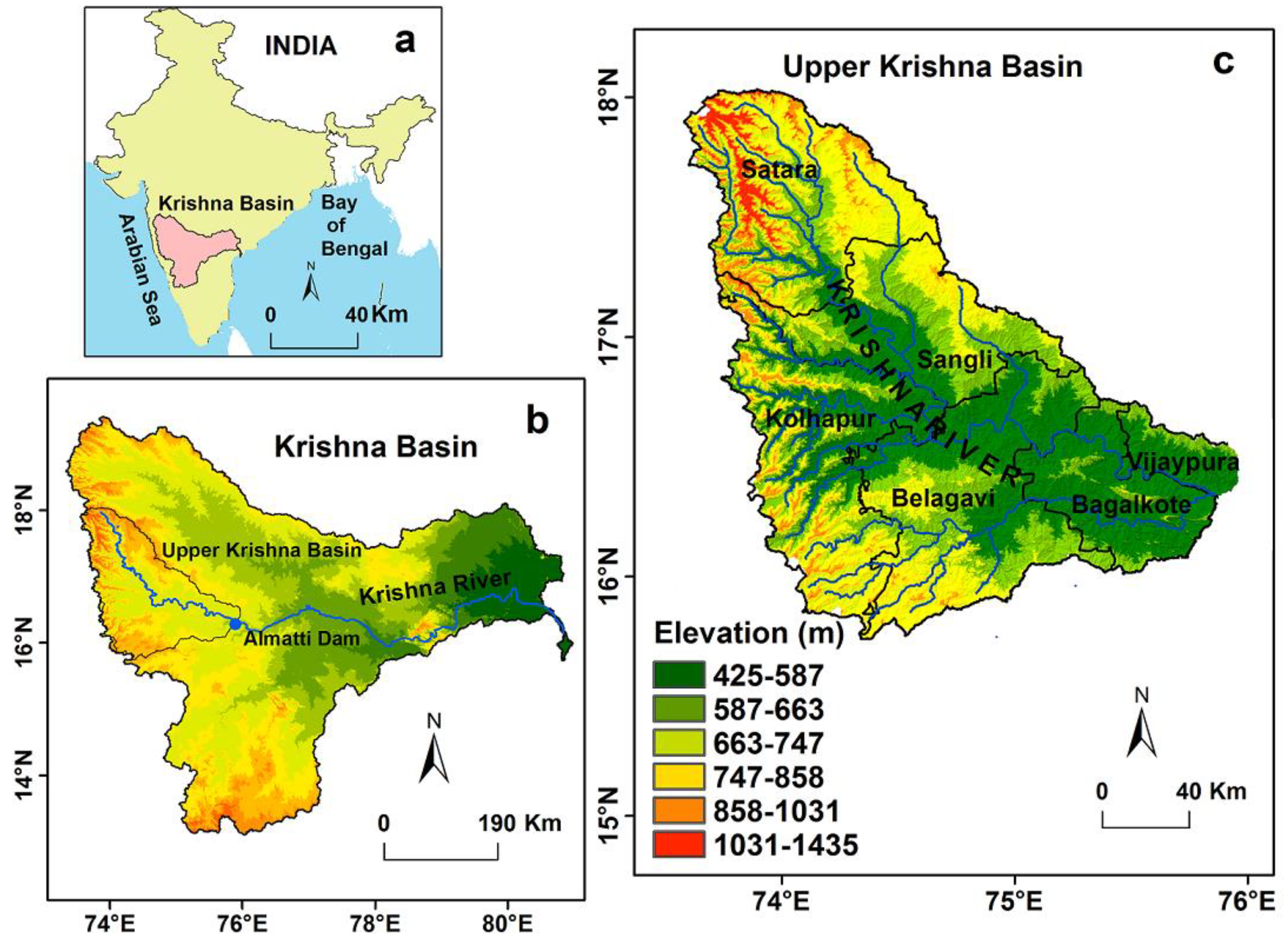
2. Study Area
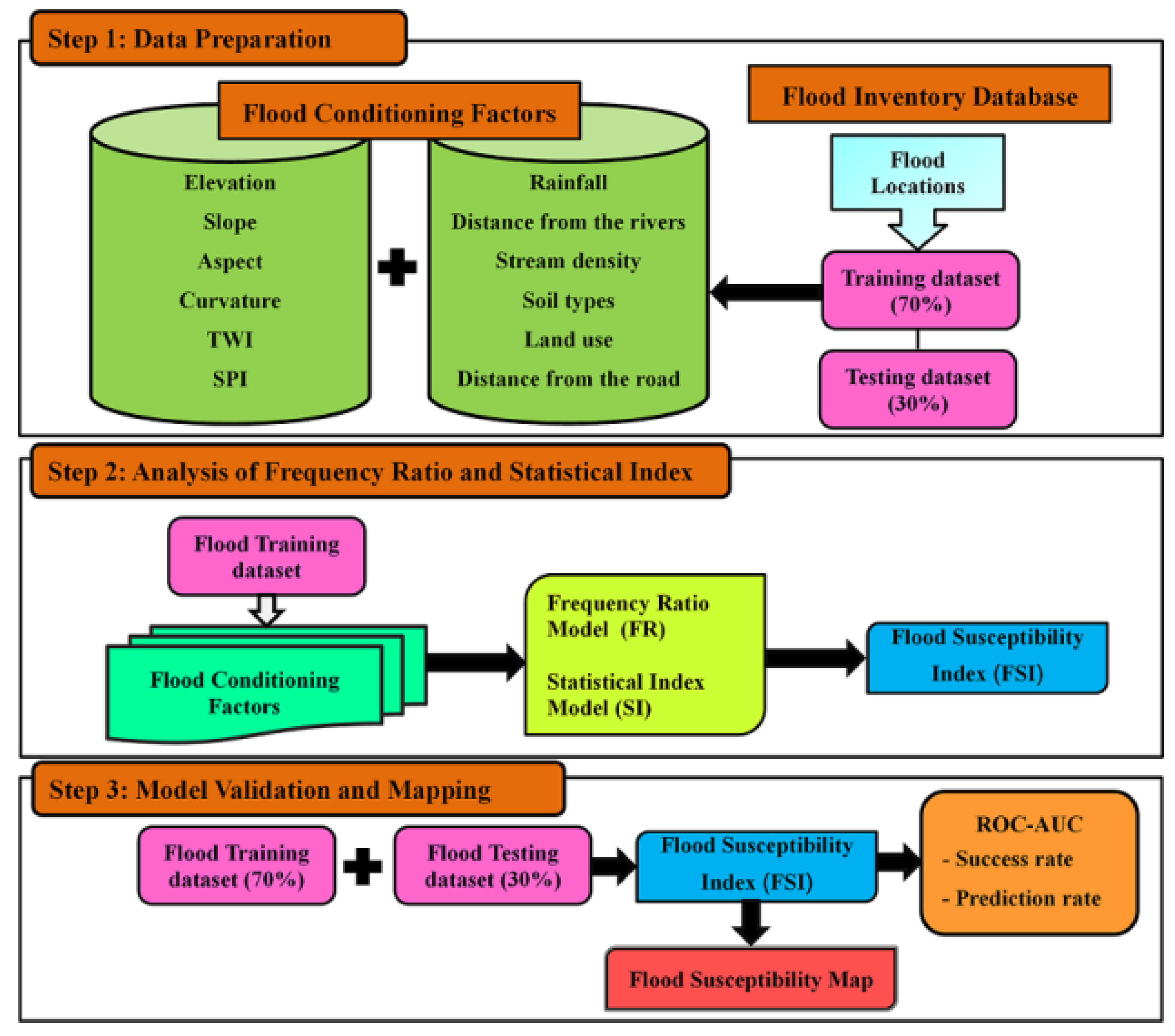
3. Materials and Methods
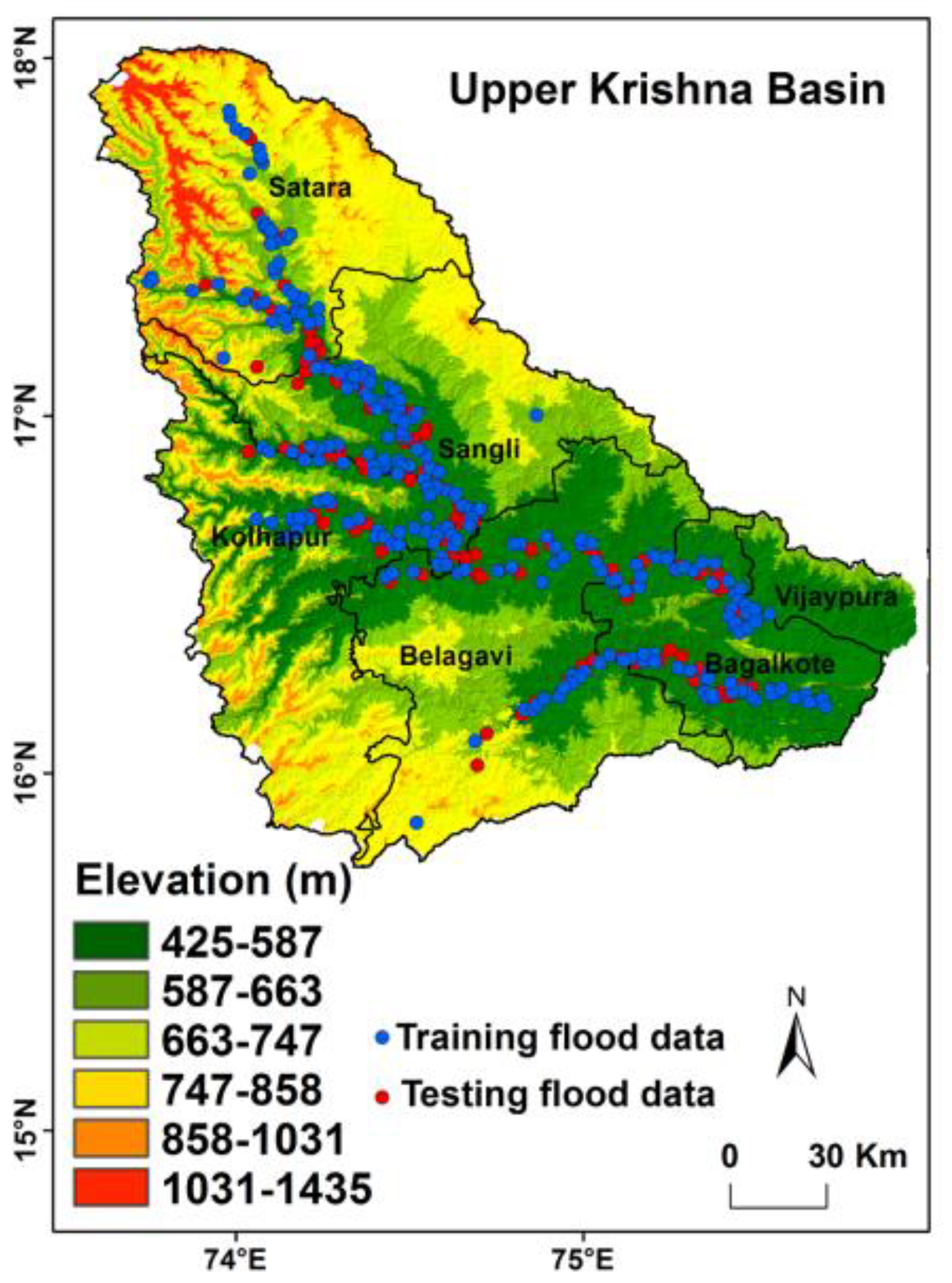
3.1. Flood Location Data
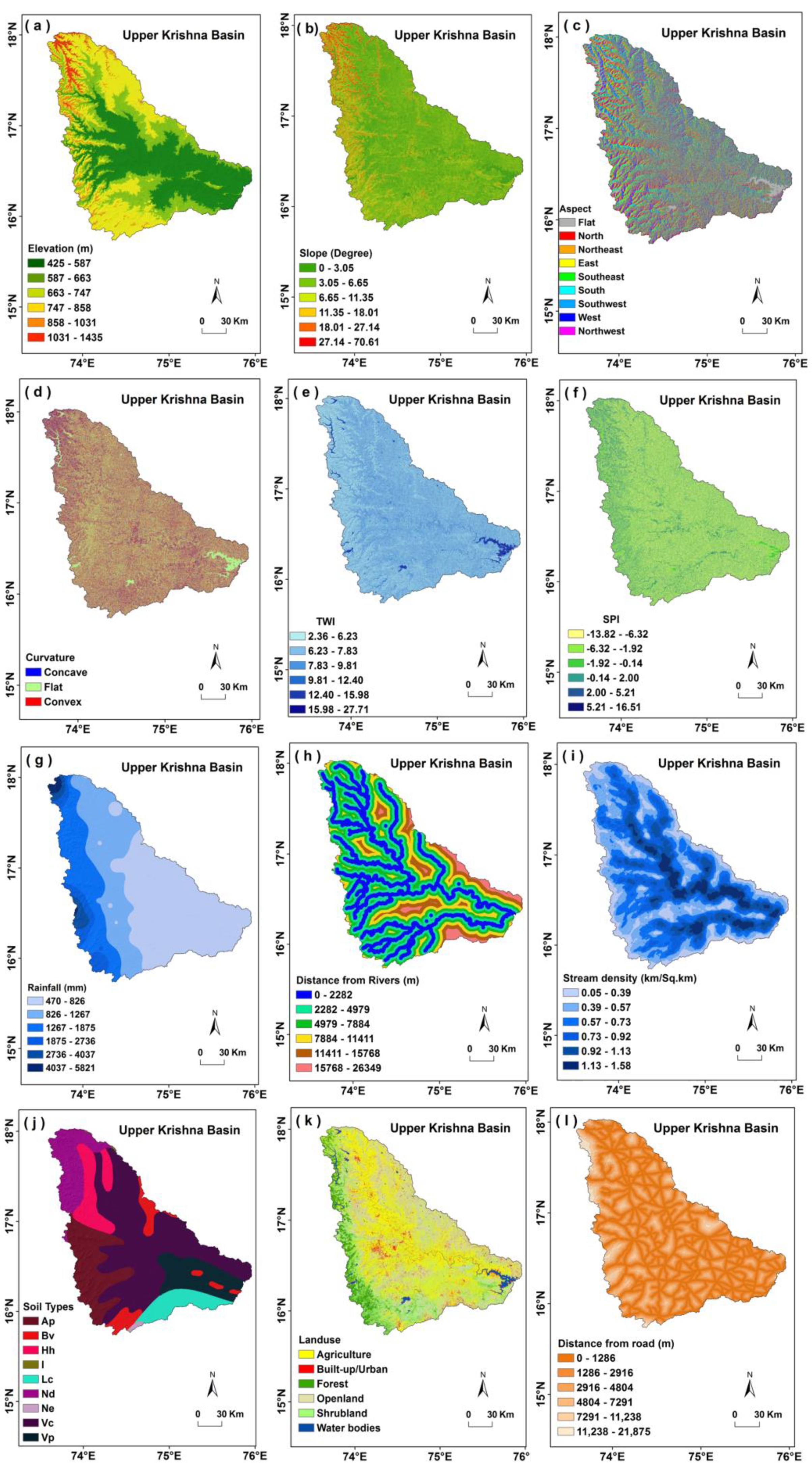
3.2. Flood Controling Factors
3.3. Frequency Ratio (FR) Model
3.4. Statistical Index (SI) Model
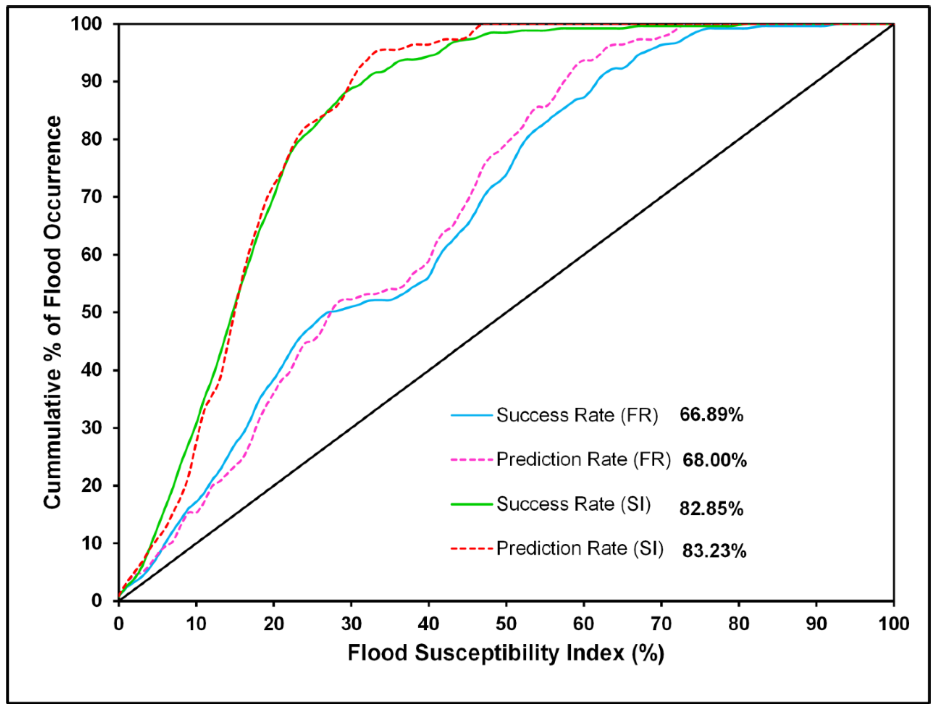
3.5. Models Validation
4. Results and Discussion
4.1. Flood Susceptibility Analysis by the Frequency Ratio Model
4.2. Flood Susceptibility Analysis by the Statistical Index Model
4.3. Flood Susceptibility Model Validation and Comparison
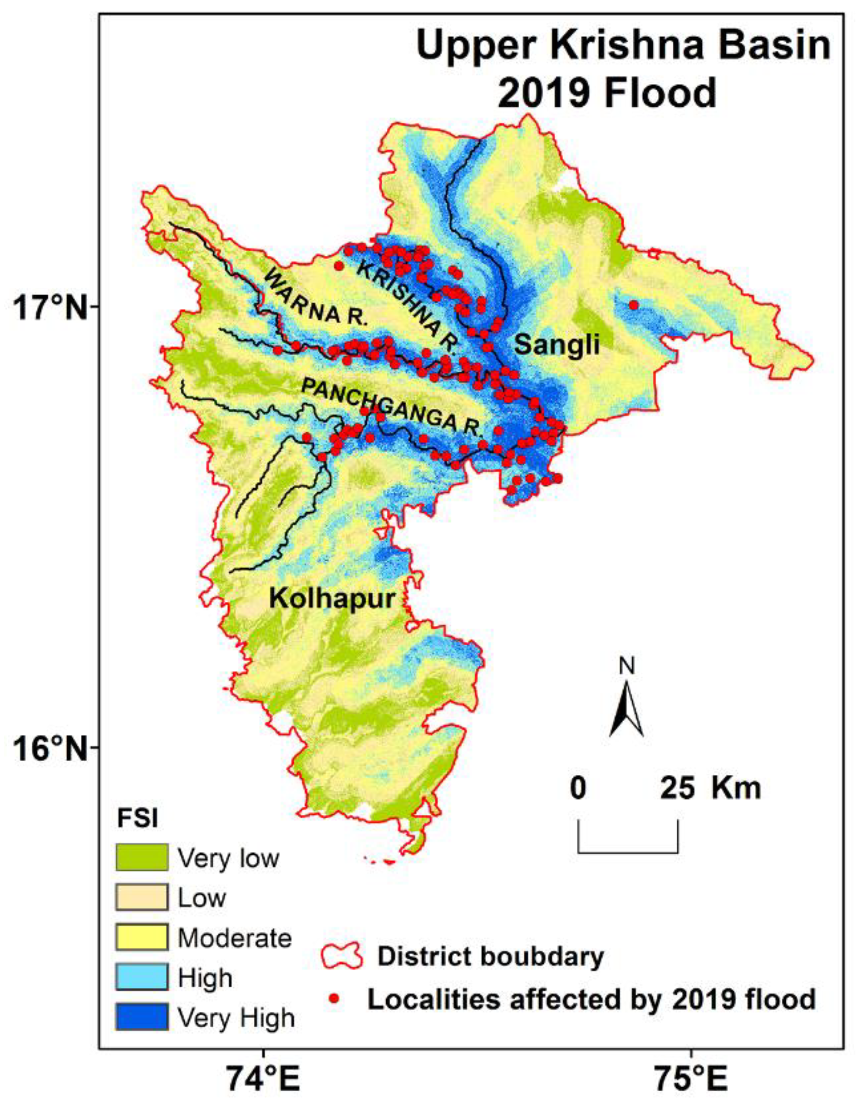
4.4. Application of the Research
5. Conclusions
Author Contributions
Funding
Data Availability Statement
Conflicts of Interest
References
- Youssef, A.M.; Pradhan, B.; Hassan, A.M. Flash flood risk estimation along the St. Katherine road, southern Sinai, Egypt using GIS based morphometry and satellite imagery. Environ. Earth Sci. 2011, 62, 611–623. [Google Scholar] [CrossRef]
- Du, J.; Fang, J.; Xu, W.; Shi, P. Analysis of dry/wet conditions using the standardized precipitation index and its potential usefulness for drought/flood monitoring in Hunan Province China. Stoch. Environ. Res. Risk Assess. 2013, 27, 377–387. [Google Scholar] [CrossRef]
- Yu, J.; Qin, X.; Larsen, O. Joint Monte Carlo and possibilistic simulation for flood damage assessment. Stoch. Environ. Res. Risk Assess. 2013, 27, 725–735. [Google Scholar] [CrossRef]
- Zou, Q.; Zhou, J.; Zhou, C.; Song, L.; Guo, J. Comprehensive flood risk assessment based on set pair analysis-variable fuzzy sets model and fuzzy AHP. Stoch. Environ. Res. Risk Assess. 2013, 27, 525–546. [Google Scholar] [CrossRef]
- Tehrany, M.S.; Shabani, F.; Jebur, M.N.; Hong, H.; Chen, W.; Xie, X. GIS-based spatial prediction of flood prone areas using standalone frequency ratio, logistic regression, weight of evidence and their ensemble techniques. Geomatics. Nat. Hazards Risk 2017, 8, 1538–1561. [Google Scholar] [CrossRef] [Green Version]
- Pawar, U.V. An Analytical Study of Geomorphological, Hydrological, and Meteorological Characteristics of Floods in the Mahi River Basin: Western India. Ph.D. Thesis, Tilak Maharashtra Vidyapeeth, Pune, India, 2019. [Google Scholar]
- Toduse, N.C.; Ungurean, C.; Davidescu, S.; Clinciu, I.; Marin, M.; Nita, M.D.; Davidescu, A. Torrential flood risk assessment and environmentally friendly solutions for small catchments located in the Romania Natura 2000 sites Ciucas, Postavaru and Mare. Sci. Total Environ. 2020, 698, 134271. [Google Scholar] [CrossRef]
- Kazakis, N.; Kougias, I.; Patsialis, T. Assessment of flood hazard areas at a regional scale using an index-based approach and Analytical Hierarchy Process: Application in Rhodope-Evros region, Greece. Sci. Total Environ. 2015, 538, 555–563. [Google Scholar] [CrossRef]
- Wang, Y.; Hong, H.; Chen, W.; Li, S.; Panahi, M.; Khosravi, K.; Shirzadi, A.; Shahabi, H.; Panahi, S.; Costache, R. Flood susceptibility mapping in Dingnan County (China) using adaptive neuro-fuzzy inference system with biogeography based optimization and imperialistic competitive algorithm. J. Environ. Manag. 2019, 247, 712–729. [Google Scholar] [CrossRef]
- Charlton, R.; Fealy, R.; Moore, S.; Sweeney, J.; Murphy, C. Assessing the impact of climate change on water supply and flood hazard in Ireland using statistical downscaling and hydrological modeling techniques. Clim. Chang. 2006, 74, 475–491. [Google Scholar] [CrossRef]
- Pawar, U.V.; Hire, P.S.; Gunjal, R.P.; Patil, A.D. Modeling of magnitude and frequency of floods on the Narmada River: India. Modeling Earth Syst. Environ. 2020, 6, 2505–2516. [Google Scholar] [CrossRef]
- Alfieri, L.; Bisselink, B.; Dottori, F.; Naumann, G.; de Roo, A.; Salamon, P.; Wyser, K.; Feyen, L. Global projections of river flood risk in a warmer world. Earth’s Future 2017, 5, 171–182. [Google Scholar] [CrossRef]
- Pradhan, B. Flood susceptible mapping and risk area delineation using logistic regression, GIS and remote sensing. J. Spat. Hydrol. 2010, 9, 1–18. [Google Scholar]
- Diakakis, M.; Mavroulis, S.; Deligiannakis, G. Floods in Greece: A statistical and spatial approach. Nat. Hazards 2012, 62, 485–500. [Google Scholar] [CrossRef]
- Huang, X.; Tan, H.; Zhou, J.; Yang, T.; Benjamin, A.; Wen, S.W.; Li, S.; Liu, A.; Li, X.; Fen, S.; et al. Flood hazard in Hunan province of China: An economic loss analysis. Nat. Hazards 2008, 47, 65–73. [Google Scholar] [CrossRef]
- Dawson, C.W.; Abrahart, R.J.; Shamseldin, A.Y.; Wilby, R.L. Flood estimation at ungauged sites using artificial neural networks. J. Hydrol. 2006, 319, 391–409. [Google Scholar] [CrossRef] [Green Version]
- Bubeck, P.; Botzen, W.; Aerts, J. A review of risk perceptions and other factors that influence flood mitigation behavior. Risk Anal. 2012, 32, 1481–1495. [Google Scholar] [CrossRef] [Green Version]
- Mandal, S.P.; Chakrabarty, A. Flash flood risk assessment for upper Teesta river basin: Using the hydrological modeling system (HEC-HMS) software. Model. Earth Syst. Environ. 2016, 2, 59. [Google Scholar] [CrossRef] [Green Version]
- Bui, D.T.; Ngo, P.T.T.; Pham, T.D.; Jaafari, A.; Minh, N.Q.; Hoa, P.V.; Samui, P. A novel hybrid approach based on a swarm intelligence optimized extreme learning machine for flash flood susceptibility mapping. Catena 2019, 179, 184–196. [Google Scholar] [CrossRef]
- Bates, P.D. Remote sensing and flood inundation modeling. Hydrol. Process. 2004, 18, 2593–2597. [Google Scholar] [CrossRef]
- Liu, J.F.; Li, J.; Liu, J.; Cao, R.Y. Integrated GIS/AHP-based flood risk assessment: A case study of Huaihe River Basin in China. J. Nat. Disasters 2008, 17, 110–114. [Google Scholar]
- Haq, M.; Akhtar, M.; Muhammad, S.; Paras, S.; Rahmatullah, J. Techniques of Remote Sensing and GIS for flood monitoring and damage assessment: A case study of Sindh Province, Pakistan. Egypt. J. Remote Sens. Space Sci. 2012, 15, 135–141. [Google Scholar] [CrossRef] [Green Version]
- Jaafari, A.; Najafi, A.; Pourghasemi, H.; Rezaeian, J.; Sattarian, A. GIS-based frequency ratio and index of entropy models for landslide susceptibility assessment in the Caspian forest, Northern Iran. Int. J. Environ. Sci. Technol. 2014, 11, 909–926. [Google Scholar] [CrossRef]
- Rahmati, O.; Zeinivand, H.; Besharat, M. Flood hazard zoning in Yasooj region, Iran, using GIS and multi criteria decision analysis. Geomat. Nat. Hazards Risk 2016, 7, 1000–1017. [Google Scholar] [CrossRef] [Green Version]
- Paul, G.C.; Saha, S.; Hembram, T.K. Application of the GIS-based probabilistic models for mapping the flood susceptibility in Bansloi sub-basin of Ganga-Bhagirathi river and their comparison. Remote Sens. Earth Syst. Sci. 2019, 2, 120–146. [Google Scholar] [CrossRef]
- Msabi, M.M.; Makonyo, M. Flood susceptibility mapping using GIS and multi-criteria decision analysis: A case of Dodoma region, central Tanzania. Remote Sens. Appl. Soc. Environ. 2021, 21, 100445. [Google Scholar] [CrossRef]
- Suppawimut, W. GIS-Based Flood Susceptibility Mapping Using Statistical Index and Weighting Factor Models. Environ. Nat. Resour. 2021, 19, 481–493. [Google Scholar] [CrossRef]
- Malczewski, J. GIS-based multicriteria decision analysis: A survey of the literature. Int. J. Geograph. Inform. Sci. 2006, 20, 703–726. [Google Scholar] [CrossRef]
- Hwang, C.L.; Lin, M.J. Group Decision Making under Multiple Criteria: Methods and Applications; Springer: Berlin/Heidelberg, Germany, 2012. [Google Scholar]
- Sarker, S.; Veremyev, A.; Boginski, V.; Singh, A. Critical nodes in river networks. Sci. Rep. 2019, 9, 11178. [Google Scholar] [CrossRef] [Green Version]
- Gao, Y.; Sarker, S.; Sarker, T.; Leta, O.T. Analyzing the critical locations in response of constructed and planned dams on the Mekong River Basin for environmental integrity. Environ. Res. Commun. 2022, 4, 101001. [Google Scholar] [CrossRef]
- Talei, A.; Chua, L.H.C.; Quek, C. A novel application of a neurofuzzy computational technique in event-based rainfall–runoff modeling. Expert Syst. Appl. 2010, 37, 7456–7468. [Google Scholar] [CrossRef]
- Kia, M.B.; Pirasteh, S.; Pradhan, B.; Mahmud, A.R.; Sulaiman, W.N.A.; Moradi, A. An artificial neural network model for flood simulation using GIS: Johor River Basin Malaysia. Environ. Earth Sci. 2012, 67, 251–264. [Google Scholar] [CrossRef]
- Cao, C.; Xu, P.; Wang, Y.; Chen, J.; Zheng, L.; Niu, C. Flash flood hazard susceptibility mapping using frequency ratio and statistical index methods in coalmine subsidence areas. Sustainability 2016, 8, 948. [Google Scholar] [CrossRef]
- Khosravi, K.; Pourghasemi, H.R.; Chapi, K.; Bahri, M. Flash flood susceptibility analysis and its mapping using different bivariate models in Iran: A comparison between Shannon’s entropy, statistical index, and weighting factor models. Environ. Monit. Assess. 2016, 188, 656. [Google Scholar] [CrossRef]
- Samanta, S.; Pal, D.K.; Palsamanta, B. Flood susceptibility analysis through remote sensing, GIS and frequency ratio model. Appl. Water Sci. 2018, 8, 66. [Google Scholar] [CrossRef] [Green Version]
- Tehrany, M.S.; Kumar, L.; Jebur, M.N.; Shabani, F. Evaluating the application of the statistical index method in flood susceptibility mapping and its comparison with frequency ratio and logistic regression methods. Geomat. Nat. Hazards Risk 2019, 10, 79–101. [Google Scholar] [CrossRef] [Green Version]
- Hoang, D.V.; Tran, H.T.; Nguyen, T.T. A GIS-based spatial multi-criteria approach for flash flood risk assessment in the Ngan Sau-Ngan Pho mountainous river basin, North Central of Vietnam. Environ. Nat. Resour. J. 2020, 18, 110–123. [Google Scholar] [CrossRef] [Green Version]
- Khaing, T.W.; Tantanee, S.; Pratoomchai, W.; Mahavik, N. Coupling flood hazard with vulnerability map for flood risk assessment: A case study of Nyaung-U Township in Myanmar. GMSARN Int. J. 2021, 15, 127–138. [Google Scholar]
- Şen, Z. Flood Modelling, Predication and Mitigation; Springer International Publishing: Cham, Switzerland, 2018. [Google Scholar] [CrossRef]
- Shrestha, R.R.; Nestmann, F. Physically based and data-driven models and propagation of input uncertainties in river flood prediction. J. Hydrol. Eng. 2009, 14, 1309–1319. [Google Scholar] [CrossRef]
- Dhar, O.N.; Nandargi, S. Hydrometeorological aspects of floods in India. Nat. Hazards 2003, 28, 1–33. [Google Scholar] [CrossRef]
- Kale, V.S. Monsoon floods in India: A hydro-geomorphic perspective. Flood studies in India. Geol. Soc. India Mem. 1998, 41, 229–256. [Google Scholar]
- Hire, P.S. Geomorphic and Hydrologic studies of Floods in the Tapi Basin. Ph.D. Thesis, University of Pune, Pune, India, 2000. [Google Scholar]
- National Institution For Transforming India (NITI). Report of the Committee Constituted for Formulation of Strategy for Flood Management Works in Entire Country and River Management Activities and Works Related to Border Areas (2021–26); National Institution for Transforming: New Delhi, India, 2021. [Google Scholar]
- Naulin, J.P.; Payrastre, O.; Gaume, E. Spatially distributed flood forecasting in flash flood prone areas: Application to road network supervision in Southern France. J. Hydrol. 2013, 486, 88–99. [Google Scholar] [CrossRef] [Green Version]
- Guo, E.; Zhang, J.; Ren, X.; Zhang, Q.; Sun, Z. Integrated risk assessment of flood disaster based on improved set pair analysis and the variable fuzzy set theory in central Liaoning Province, China. Nat. Hazards 2014, 74, 947–965. [Google Scholar] [CrossRef]
- Ullah, K.; Zhang, J. GIS-based flood hazard mapping using relative frequency ratio method: A case study of Panjkora River Basin, eastern Hindu Kush, Pakistan. PLoS ONE 2020, 15, e0229153. [Google Scholar] [CrossRef] [PubMed]
- Chanapathi, T.; Thatikonda, S.; Raghavan, S. Analysis of rainfall extremes and water yield of Krishna river basin under future climate scenarios. J. Hydrol. Reg. Stud. 2018, 19, 287–306. [Google Scholar] [CrossRef]
- Rakhecha, P.R.; Deshpande, N.R.; Kulkarni, A.K.; Mandal, B.N.; Sangam, R.B. Design Storm Studies for the Upper Krishna River Catchment Upstream of the Almatti dam site. Theor. Appl. Climatol. 1995, 52, 219–229. [Google Scholar] [CrossRef]
- WRD. Integrated State Water Plan for Upper Krishna (k-1) Sub-Basin; WRD: Maharashtra, India, 2015; pp. 1–519. [Google Scholar]
- GOM. Expert Study Committee Report: Floods 2019 (Krishna Basin); GOM: Maharashtra, India, 2020; pp. 1–190. [Google Scholar]
- GOK. Seeking Central Assistance for Relief and Emergency Works Due to Flood and Landslides in Karnataka during August 2019. In Memorandum; GOK: Karnataka, India, 2019; pp. 1–209. [Google Scholar]
- Ali, S.A.; Khatun, R.; Ahmad, A.; Ahmad, S.N. Application of GIS-based analytic hierarchy process and frequency ratio model to flood vulnerable mapping and risk area estimation at Sundarban region, India. Model. Earth Syst. Environ. 2019, 5, 1083–1102. [Google Scholar] [CrossRef]
- Chowdhuri, I.; Pal, S.; Chakrabortty, R. Flood susceptibility mapping by ensemble evidential belief function and binomial logistic regression model on river basin of eastern India. Adv. Space Res. 2020, 65, 1466–1489. [Google Scholar] [CrossRef]
- Vafakhah, M.; Mohammad Hasani Loor, S.; Pourghasemi, H.; Katebikord, A. Comparing performance of random forest and adaptive neuro-fuzzy inference system data mining models for flood susceptibility mapping. Arabian J. Geosci 2020, 13, 11. [Google Scholar] [CrossRef]
- Mahato, S.; Pal, S.; Talukdar, S.; Saha, T.; Mandal, P. Field based index of flood vulnerability (IFV): A new validation technique for flood susceptible models. Geosci. Front. 2021, 12, 101175. [Google Scholar] [CrossRef]
- Hasanuzzaman, M.; Adhikary, P.; Bera, B.; Shit, P. Flood vulnerability assessment using AHP and frequency ratio techniques. In Spatial Modelling of Flood Risk and Flood Hazards; Springer Nature: Cham, Switzerland, 2022; p. 91. [Google Scholar] [CrossRef]
- Pradhan, B.; Tehrany, M.S.; Jebur, M.N. A new semi-automated detection mapping of flood extent from TerraSAR-X satellite image using rule-based classification and Taguchi optimization techniques. IEEE Trans. Geosci. Remote Sens. 2016, 54, 4331–4342. [Google Scholar] [CrossRef]
- Nguyen, V.N.; Yariyan, P.; Amiri, M.; Dang Tran, A.; Pham, T.D.; Do, M.P.; Tien Bui, D. A new modeling approach for spatial prediction of flash flood with biogeography optimized CHAID tree ensemble and remote sensing data. Remote Sens. 2020, 12, 1373. [Google Scholar] [CrossRef]
- Souissi, D.; Zouhri, L.; Hammami, S.; Msaddek, M.H.; Zghibi, A.; Dlala, M. GIS-based MCDM–AHP modeling for flood susceptibility mapping of arid areas, Southeastern Tunisia. Geocarto Int. 2020, 35, 991–1017. [Google Scholar] [CrossRef]
- Bathrellos, G.D.; Skilodimou, H.D.; Soukis, K.; Koskeridou, E. Temporal and spatial analysis of flood occurrences in the drainage basin of Pinios river (Thessaly, Central Greece). Land 2018, 7, 106. [Google Scholar] [CrossRef] [Green Version]
- Young, R.A.; Mutchler, C.K. Effect of slope shape on erosion and runoff. Trans. ASAE 1969, 12, 0231–0233. [Google Scholar] [CrossRef]
- Hudson, P.F.; Kesel, R.H. Channel migration and meander-bend curvature in the lower Mississippi River prior to major human modification. Geology 2000, 28, 531–534. [Google Scholar] [CrossRef]
- Qin, C.Z.; Zhu, A.X.; Pei, T.; Li, B.L.; Scholten, T.; Behrens, T.; Zhou, C.H. An approach to computing topographic wetness index based on maximum downslope gradient. Precis. Agric. 2011, 12, 32–43. [Google Scholar] [CrossRef]
- Jebur, M.N.; Pradhan, B.; Tehrany, M.S. Optimization of landslide conditioning factors using very high-resolution airborne laser scanning (LiDAR) data at catchment scale. Remote Sens. Environ. 2014, 152, 150–165. [Google Scholar] [CrossRef]
- Patil, A.D.; Hire, P.S. Flood hydrometeorological situations associated with monsoon floods on the Par River in western India. Mausam 2021, 71, 687–698. [Google Scholar]
- Pawar, U.; Rathnayake, U. Spatiotemporal rainfall variability and trend analysis over Mahaweli Basin, Sri Lanka. Arab. J. Geosci. 2022, 15, 370–416. [Google Scholar] [CrossRef]
- Pawar, U.; Karunathilaka, P.; Rathnayake, U. Spatio-Temporal Rainfall Variability and Concentration over Sri Lanka. Adv. Meteorol. 2022, 2022, 6456761. [Google Scholar] [CrossRef]
- Shekhar, S.; Pandey, A.C. Delineation of groundwater potential zone in hard rock terrain of India using remote sensing, geographical information system (GIS) and analytic hierarchy process (AHP) techniques. Geocarto. Int. 2015, 30, 402–421. [Google Scholar] [CrossRef]
- Capon, S.J. Flood variability and spatial variation in plant community composition and structure on a large arid floodplain. J. Arid. Environ. 2005, 60, 283–302. [Google Scholar] [CrossRef]
- Chaplot, V.; Poesen, J. Sediment, soil organic carbon and runoff delivery at various spatial scales. Catena 2012, 88, 46–56. [Google Scholar] [CrossRef]
- Hölting, B.; Coldewey, W.G. Surface water infiltration. In Hydrogeology; Springer: Berlin/Heidelberg, Germany, 2019; pp. 33–37. [Google Scholar]
- Chen, Y.; Liu, R.; Barrett, D.; Gao, L.; Zhou, M.; Renzullo, L.; Emelyanova, I. A spatial assessment framework for evaluating flood risk under extreme climates. Sci. Total Environ. 2015, 538, 512–523. [Google Scholar] [CrossRef]
- Youssef, A.M.; Pradhan, B.; Sefry, S.A. Flash flood susceptibility assessment in Jeddah city (Kingdom of Saudi Arabia) using bivariate and multivariate statistical models. Environ. Earth Sci. 2016, 75, 1–16. [Google Scholar] [CrossRef]
- Hammami, S.; Zouhri, L.; Souissi, D.; Souei, A.; Zghibi, A. Application of the GIS based multi-criteria decision analysis and analytical hierarchy process (AHP) in the flood susceptibility mapping (Tunisia). Arab. J. Geosci. 2019, 12, 653. [Google Scholar] [CrossRef]
- Roslee, R.; Tongkul, F.; Mariappan, S.; Simon, N. Flood hazard analysis (FHAn) using multi-criteria evaluation (MCE) in Penampang Area, Sabah Malaysia. ASM Sci. J. 2018, 11, 104–122. [Google Scholar]
- Yalcin, A.; Reis, S.; Aydinoglu, A.C.; Yomralioglu, T. A GIS-based comparative study of frequency ratio, analytical hierarchy process, bivariate statistics and logistic regression methods for landslide susceptibility mapping in Trabzon, NE Turkey. Catena 2011, 85, 274–287. [Google Scholar] [CrossRef]
- Wu, Y.; Li, W.; Wang, Q.; Liu, Q.; Yang, D.; Xing, M.; Pei, Y.; Yan, S. Landslide Susceptibility Assessment Using Frequency Ratio, Statistical Index and Certainty Factor Models for the Gangu County, China. Arab. J. Geosci. 2016, 9, 84. [Google Scholar] [CrossRef]
- Tiwari, A.; Shoab, M.; Dixit, A. GIS-based forest fire susceptibility modeling in Pauri Garhwal, India: A comparative assessment of frequency ratio, analytic hierarchy process and fuzzy modeling techniques. Nat. Hazards 2021, 105, 1189–1230. [Google Scholar] [CrossRef]
- Rehman, A.; Song, J.; Haq, F.; Mahmood, S.; Ahamad, M.I.; Basharat, M.; Sajid, M.; Mehmood, M.S. Multi-Hazard Susceptibility Assessment Using the Analytical Hierarchy Process and Frequency Ratio Techniques in the Northwest Himalayas, Pakistan. Remote Sens. 2022, 14, 554. [Google Scholar] [CrossRef]
- Westen, C.J.V. Statistical Landslide Hazard Analysis. ILWIS 2.1 for Windows Application Guide; ITC Publication: Enschede, The Netherlands, 1997; pp. 73–84. [Google Scholar]
- Ali, S.A.; Parvin, F.; Pham, Q.B.; Vojtek, M.; Vojteková, J.; Costache, R.; Thuy Linh, N.T.; Nguyen, H.Q.; Ahmad, A.; Ghorbani, M.A. GIS-Based Comparative Assessment of Flood Susceptibility Mapping Using Hybrid Multi-Criteria Decision-Making Approach, Naïve Bayes Tree, Bivariate Statistics and Logistic Regression: A Case of Topla Basin, Slovakia. Ecol. Indic. 2020, 117, 106620. [Google Scholar] [CrossRef]
- Rossi, M.; Reichenbach, P. LAND-SE: Software for statistically based landslide susceptibility zonation, version 1.0. Geosci. Model. Dev. 2016, 9, 3533–3543. [Google Scholar] [CrossRef] [Green Version]
- Wahono, B.F.D. Applications of statistical and heuristic methods for landslide susceptibility assessments: A case study in Wadas Lintang Sub District, Wonosobo Regency, Central Java Province, Indonesia. Ph.D. Thesis, Gadjah Mada University, Sleman, Indonesia, 2010; pp. 12–37. [Google Scholar]
- Pimiento, E. Shallow landslide susceptibility: Modelling and validation. Ph.D. Thesis, Lund University, Lund, Sweden, 2010; pp. 25–29. [Google Scholar]
- Silalahi, F.E.S.; Pamela; Arifianti, Y.; Hidayat, F. Landslide susceptibility assessment using frequency ratio model in Bogor, West Java, Indonesia. Geosci. Lett. 2019, 6, 10. [Google Scholar] [CrossRef]
- Jaiswal, R.K.; Mukherjee, S.; Krishnamurthy, J.; Saxena, R. Role of remote sensing and GIS techniques for generation of groundwater prospect zones towards rural development—An approach. Int. J. Remote Sens. 2003, 24, 993–1008. [Google Scholar] [CrossRef]
- Sharif, H.O.; Al-Juaidi, F.H.; Al-Othman, A.; Al-Dousary, I.; Fadda, E.; Jamal-Uddeen, S.; Elhassan, A. Flood hazards in an urbanizing watershed in Riyadh, Saudi Arabia. Geomat. Nat. Hazards Risk 2016, 7, 702–720. [Google Scholar] [CrossRef] [Green Version]
- Dudal, R. Dark Clay Soils of Tropical and Subtropical Regions; FAO Agricultural Development Paper No. 83; FAO: Rome, Italy, 1965. [Google Scholar]
- De Vos, J.H.; Virgo, K.J. Soil structure in vertisols of the Blue Nile clay plains, Sudan. Eur. J. Soil Sci. 1969, 20, 189–206. Available online: https://www.thehindu.com/news/national/other-states/floods-paralyse-kolhapur-sangli-132-lakh-evacuated/article28873771.ece (accessed on 27 October 2022). [CrossRef]


| Flood Conditioning Factors | Data Type | Descriptions | Source |
|---|---|---|---|
| Elevation | Raster grid | Derived from ASTER DEM (30 m × 30 m) using ArcGIS | USGS https://earthexplorer.usgs.gov (accessed on 23 August 2022) |
| Slope | |||
| Aspect | |||
| Curvature | |||
| TWI | |||
| SPI | |||
| Rainfall | Attribute data | Derived from raingauge rainfall data and converted into raster data with 30 m × 30 m cell size | Department of Agriculture, Maharashtra, India Meteorological Department, and Karnataka Sate Natural Disaster Monitoring Center, India |
| Distance from the river | Vector data (Line) | Derived from stream networks of the UKB (30 m × 30 m) using ArcGIS | USGS https://earthexplorer.usgs.gov (accessed on 23 August 2022) |
| Stream density | Raster grid | Derived from ASTER DEM (30 m × 30 m) using fill, flow accumulation, drainage density command in ArcGIS | USGS https://earthexplorer.usgs.gov (accessed on 23 August 2022) |
| Soil types | Vector data (Polygon) | Digital soil map of the world-ESRI shape file | FAO http://www.fao.org (accessed on 22 August) |
| Land use | Raster grid | Landsat 8 OLI/TIRS, 30 m × 30 m | USGS https://earthexplorer.usgs.gov (accessed on 25 August 2022) |
| Distance from the road | Vector data (Line) | Derived from road networks of the district and converted into raster data with 30 m × 30 m cell size | DIVA-GIS https://www.diva-gis.org › gdata (accessed on 23 August 2022) |
| Flood inventory database | Vector data (Point) | Google Earth and Reports | Electronic Media (News), Print Media (Newspaper), Social Media, and Published Reports |
| Factors | Class | No. Pixels | Area (%) | Floods Pixels | Flood (%) | Frequency Ratio (FR) | Stastical Index (SI) |
|---|---|---|---|---|---|---|---|
| Elevation (m) | 425–587 | 13685981 | 37.58 | 225 | 86.87 | 2.31 | 84 |
| 587–663 | 9331587 | 25.62 | 28 | 10.81 | 0.42 | −86 | |
| 663–747 | 6918565 | 19.00 | 5 | 1.93 | 0.10 | −229 | |
| 747–858 | 4221014 | 11.59 | 1 | 0.39 | 0.03 | −340 | |
| 858–1031 | 1703324 | 4.68 | 0 | 0.00 | 0.00 | 0 | |
| 1031–1435 | 559906 | 1.54 | 0 | 0.00 | 0.00 | 0 | |
| Slope (degree) | 0–3.05 | 12859597 | 35.31 | 69 | 26.64 | 0.75 | −28 |
| 3.05–6.65 | 13741170 | 37.73 | 135 | 52.12 | 1.38 | 32 | |
| 6.65–11.35 | 5703779 | 15.66 | 50 | 19.31 | 1.23 | 21 | |
| 11.35–18.01 | 2382527 | 6.54 | 5 | 1.93 | 0.30 | −122 | |
| 18.01–27.14 | 1226979 | 3.37 | 0 | 0.00 | 0.00 | 0 | |
| 27.14–70.61 | 506325 | 1.39 | 0 | 0.00 | 0.00 | 0 | |
| Aspect | Flat | 3989717 | 10.95 | 19 | 7.34 | 0.67 | −40 |
| North | 7311702 | 20.08 | 26 | 10.04 | 0.50 | −69 | |
| Northeast | 3589296 | 9.86 | 25 | 9.65 | 0.98 | −2 | |
| East | 3794366 | 10.42 | 27 | 10.42 | 1.00 | 0 | |
| Southeast | 4130598 | 11.34 | 36 | 13.90 | 1.23 | 20 | |
| South | 3568439 | 9.80 | 25 | 9.65 | 0.99 | −1 | |
| Southwest | 3628161 | 9.96 | 43 | 16.60 | 1.67 | 51 | |
| West | 3274717 | 8.99 | 32 | 12.36 | 1.37 | 32 | |
| Northwest | 3133381 | 8.60 | 26 | 10.04 | 1.17 | 15 | |
| Curvature | Convex | 3903486 | 10.72 | 16 | 6.18 | 0.58 | −55 |
| Flat | 20857583 | 57.27 | 146 | 56.37 | 0.98 | −2 | |
| Concave | 11659308 | 32.01 | 97 | 37.45 | 1.17 | 16 | |
| Topographic Wetness Index (TWI) | 2.36–6.23 | 11479372 | 31.52 | 117 | 45.17 | 1.43 | 36 |
| 6.23–7.83 | 13937655 | 38.27 | 106 | 40.93 | 1.07 | 7 | |
| 7.83–9.81 | 6107429 | 16.77 | 25 | 9.65 | 0.58 | −55 | |
| 9.81–12.40 | 3013928 | 8.28 | 7 | 2.70 | 0.33 | −112 | |
| 12.40–15.98 | 1604271 | 4.40 | 4 | 1.54 | 0.35 | −105 | |
| 15.98–27.71 | 277722 | 0.76 | 0 | 0.00 | 0.00 | 0 | |
| Stream Power Index (SPI) | −13.82–−6.32 | 15348035 | 42.14 | 159 | 61.39 | 1.46 | 38 |
| −6.32–−1.92 | 5347891 | 14.68 | 34 | 13.13 | 0.89 | −11 | |
| −1.92–−0.14 | 8268133 | 22.70 | 48 | 18.53 | 0.82 | −20 | |
| −0.14–2.00 | 4989706 | 13.70 | 13 | 5.02 | 0.37 | −100 | |
| 2.00–5.21 | 2027553 | 5.57 | 5 | 1.93 | 0.35 | −106 | |
| 5.21–16.51 | 439059 | 1.21 | 0 | 0.00 | 0.00 | 0 | |
| Rainfall (mm) | 470–826 | 16998500 | 46.67 | 155 | 59.85 | 1.28 | 25 |
| 826–1267 | 9985786 | 27.42 | 85 | 32.82 | 1.20 | 18 | |
| 1267–1875 | 6621008 | 18.18 | 19 | 7.34 | 0.40 | −91 | |
| 1875–2736 | 1759703 | 4.83 | 0 | 0.00 | 0.00 | 0 | |
| 2736–4037 | 777959 | 2.14 | 0 | 0.00 | 0.00 | 0 | |
| 4037–5821 | 277421 | 0.76 | 0 | 0.00 | 0.00 | 0 | |
| Distance from rivers (m) | 0–2282 | 10494750 | 28.82 | 226 | 87.26 | 3.03 | 111 |
| 2282–4979 | 9609658 | 26.39 | 27 | 10.42 | 0.40 | −93 | |
| 4979–7884 | 7927304 | 21.77 | 3 | 1.16 | 0.05 | −293 | |
| 7884–11,411 | 4973052 | 13.65 | 2 | 0.77 | 0.06 | −287 | |
| 11,411–15,768 | 2584543 | 7.10 | 1 | 0.39 | 0.05 | 0 | |
| 15,768–26,349 | 831070 | 2.28 | 0 | 0.00 | 0.00 | 0 | |
| Stream density (km/sq.km) | 0.05–0.39 | 5594652 | 15.36 | 2 | 0.77 | 0.05 | −299 |
| 0.39–0.57 | 9414604 | 25.85 | 3 | 1.16 | 0.04 | −311 | |
| 0.57–0.73 | 7693109 | 21.12 | 13 | 5.02 | 0.24 | −144 | |
| 0.73–0.92 | 6566155 | 18.03 | 55 | 21.24 | 1.18 | 16 | |
| 0.92–1.13 | 4719547 | 12.96 | 95 | 36.68 | 2.83 | 104 | |
| 1.13–1.58 | 2432310 | 6.68 | 91 | 35.14 | 5.26 | 166 | |
| Soil Types | Ap | 5527500 | 15.18 | 9 | 3.47 | 0.23 | −147 |
| Bv | 1943925 | 5.34 | 1 | 0.39 | 0.07 | −263 | |
| Hh | 3172624 | 8.71 | 35 | 13.51 | 1.55 | 44 | |
| l | 28852 | 0.08 | 0 | 0.00 | 0.00 | 0 | |
| Lc | 2468282 | 6.78 | 1 | 0.39 | 0.06 | −287 | |
| Nd | 3963555 | 10.88 | 6 | 2.32 | 0.21 | −155 | |
| Ne | 120372 | 0.33 | 0 | 0.00 | 0.00 | 0 | |
| Vc | 15251970 | 41.88 | 129 | 49.81 | 1.19 | 17 | |
| Vp | 3943297 | 10.83 | 78 | 30.12 | 2.78 | 102 | |
| Land use | Agriculture | 14170930 | 38.91 | 51 | 19.69 | 0.51 | −68 |
| Built-up/Urban | 1431623 | 3.93 | 136 | 52.51 | 13.36 | 259 | |
| Forest | 2561431 | 7.03 | 0 | 0.00 | 0.00 | 0 | |
| Open Land | 10295513 | 28.27 | 62 | 23.94 | 0.85 | −17 | |
| Shrub Land | 7096236 | 19.49 | 10 | 3.86 | 0.20 | −162 | |
| Water Bodies | 863184 | 2.37 | 0 | 0.00 | 0.00 | 0 | |
| Distance from road (m) | 0–1286 | 12581331 | 34.54 | 101 | 39.00 | 1.13 | 12 |
| 1286–2916 | 11188412 | 30.72 | 92 | 35.52 | 1.16 | 15 | |
| 2916–4804 | 7174183 | 19.70 | 43 | 16.60 | 0.84 | −17 | |
| 4804–7291 | 3823147 | 10.50 | 20 | 7.72 | 0.74 | −31 | |
| 7291–11,238 | 1329214 | 3.65 | 3 | 1.16 | 0.32 | −115 | |
| 11,238–21,875 | 324090 | 0.89 | 0 | 0.00 | 0.00 | 0 |
Publisher’s Note: MDPI stays neutral with regard to jurisdictional claims in published maps and institutional affiliations. |
© 2022 by the authors. Licensee MDPI, Basel, Switzerland. This article is an open access article distributed under the terms and conditions of the Creative Commons Attribution (CC BY) license (https://creativecommons.org/licenses/by/4.0/).
Share and Cite
Pawar, U.; Suppawimut, W.; Muttil, N.; Rathnayake, U. A GIS-Based Comparative Analysis of Frequency Ratio and Statistical Index Models for Flood Susceptibility Mapping in the Upper Krishna Basin, India. Water 2022, 14, 3771. https://doi.org/10.3390/w14223771
Pawar U, Suppawimut W, Muttil N, Rathnayake U. A GIS-Based Comparative Analysis of Frequency Ratio and Statistical Index Models for Flood Susceptibility Mapping in the Upper Krishna Basin, India. Water. 2022; 14(22):3771. https://doi.org/10.3390/w14223771
Chicago/Turabian StylePawar, Uttam, Worawit Suppawimut, Nitin Muttil, and Upaka Rathnayake. 2022. "A GIS-Based Comparative Analysis of Frequency Ratio and Statistical Index Models for Flood Susceptibility Mapping in the Upper Krishna Basin, India" Water 14, no. 22: 3771. https://doi.org/10.3390/w14223771