
The Sensitivity of Meteorological Dynamics to the Variability in Catchment Characteristics


1
Africa Center of Excellence for Water Management, College of Natural and Computational Sciences, Addis Ababa University, Addis Ababa P.O. Box 1176, Ethiopia
2
National Drought Mitigation Center, School of Natural Resources, University of Nebraska-Lincoln, 815 Hardin Hall, 3310 Holdrege St., Lincoln, NE 68583-0749, USA
3
Department of Civil Engineering, Addis Ababa Science and Technology University, Addis Ababa P.O. Box 16417, Ethiopia
4
Department of Hydraulic and Water Resource Engineering, Gondar University, Gondar P.O. Box 196, Ethiopia
*
Author to whom correspondence should be addressed.
Water 2022, 14(22), 3776; https://doi.org/10.3390/w14223776
Submission received: 23 October 2022
/
Revised: 12 November 2022
/
Accepted: 16 November 2022
/
Published: 20 November 2022
(This article belongs to the Special Issue Drought Monitoring and Forecasting at Regional and Global Scale Using Remote Sensing, Ground Observations and Global Climate Datasets)
Abstract
:Evaluating meteorological dynamics is a challenging task due to the variability in hydro-climatic settings. This study is designed to assess the sensitivity of precipitation and temperature dynamics to catchment variability. The effects of catchment size, land use/cover change, and elevation differences on precipitation and temperature variability were considered to achieve the study objective. The variability in meteorological parameters to the catchment characteristics was determined using the coefficient of variation on the climate data tool (CDT). A land use/cover change and terrain analysis was performed on Google Earth Engine (GEE) and ArcGIS. In addition, a correlation analysis was performed to identify the relative influence of each catchment characteristic on the meteorological dynamics. The results of this study showed that the precipitation dynamics were found to be dominantly influenced by the land use/cover change with a correlation of 0.65, followed by the elevation difference with a correlation of −0.47. The maximum and minimum temperature variations, on the other hand, were found to be most affected by the elevation difference, with Pearson correlation coefficients of −0.53 and −0.57, respectively. However, no significant relationship between catchment size and precipitation variability was observed. In general, it is of great importance to understand the relative and combined effects of catchment characteristics on local meteorological dynamics for sustainable water resource management.
1. Introduction
Precipitation and temperature (hereafter referred to as meteorological variables) dynamics are still issues that need to be addressed by the scientific community [1]. The dynamic nature of meteorological variables, mainly precipitation and temperature, makes the challenge more complex. It has been projected that as the planet warms, climate and weather variability will increase. However, the variability in meteorological variables cannot be consistent over time [2,3,4,5]. The inconsistencies of meteorological parameter variability can be caused by catchment characteristics and global climate change. The variation in catchment characteristics such as topography and land use/cover has an impact on the variability in meteorological variables such as precipitation and temperature on a local scale. Evaluating the meteorological variability at the local scale in relation to various watershed characteristics is crucial for sustainable water resource management.
Several studies have been conducted to better understand the relationship between specific catchment characteristics and meteorological variable variability [6,7,8,9]. The authors of [6,10] looked into the relationship between land use/cover change and meteorological variability and found a strong correlation. For example, changes in land cover have an impact on the weather and climate by affecting the movement of energy, water, and greenhouse gases between the land and the atmosphere [11]. While reforestation might provide localized cooling, urban areas are expected to continue warming. According to the authors of [12], inappropriate land use changes are a major cause of climate change. Several studies have also reported a relationship between topography and the variability in meteorological variables. For example, the authors of [13] examined the characteristics of temperature variability with terrain elevation and observed a −0.865 correlation between the temperature change rate and the elevation. This study evaluated the rank of the correlation between elevation, longitude, latitude, topographic position, surface roughness, and temperature variability and found that altitude had the most noticeable effect on temperature variability, followed by latitude and longitude.
Quantifying the spatiotemporal dynamics of meteorological variables with catchment characteristics is of great importance for improved climate projections and sustainable water resource management; thus, this area needs more attention. A few studies have been reported on the individual impacts of land use/cover change on rainfall variability [6,10,12], the relationship between catchment size and rainfall variability [8,14], and the relationship between elevation and rainfall variability [9,14]. Moreover, the effects of watershed characteristics on streamflow variability [15] and the effects of catchment characteristics on predicting the hydrological sensitivity to climate change [16] have also been studied. However, to the best of our knowledge, there has been no research on an investigation of the sensitivity of meteorological dynamics to the relative variability in catchment characteristics. To fill this gap, three catchment characteristics, catchment size, topography, and land use/cover change, were selected in this study, while precipitation and temperature were selected as the meteorological variables based on data availability.
In general, this study attempted to investigate (i) the individual relationships between land use/cover change, topography, and catchment size with precipitation and temperature variations; (ii) the relative impact of these catchment characteristics on temperature and precipitation variability; and (iii) how well the dynamics of meteorological variables correspond to changes in the catchment characteristics in the Baro basin.
2. Methods and Data Description
2.1. Study Area
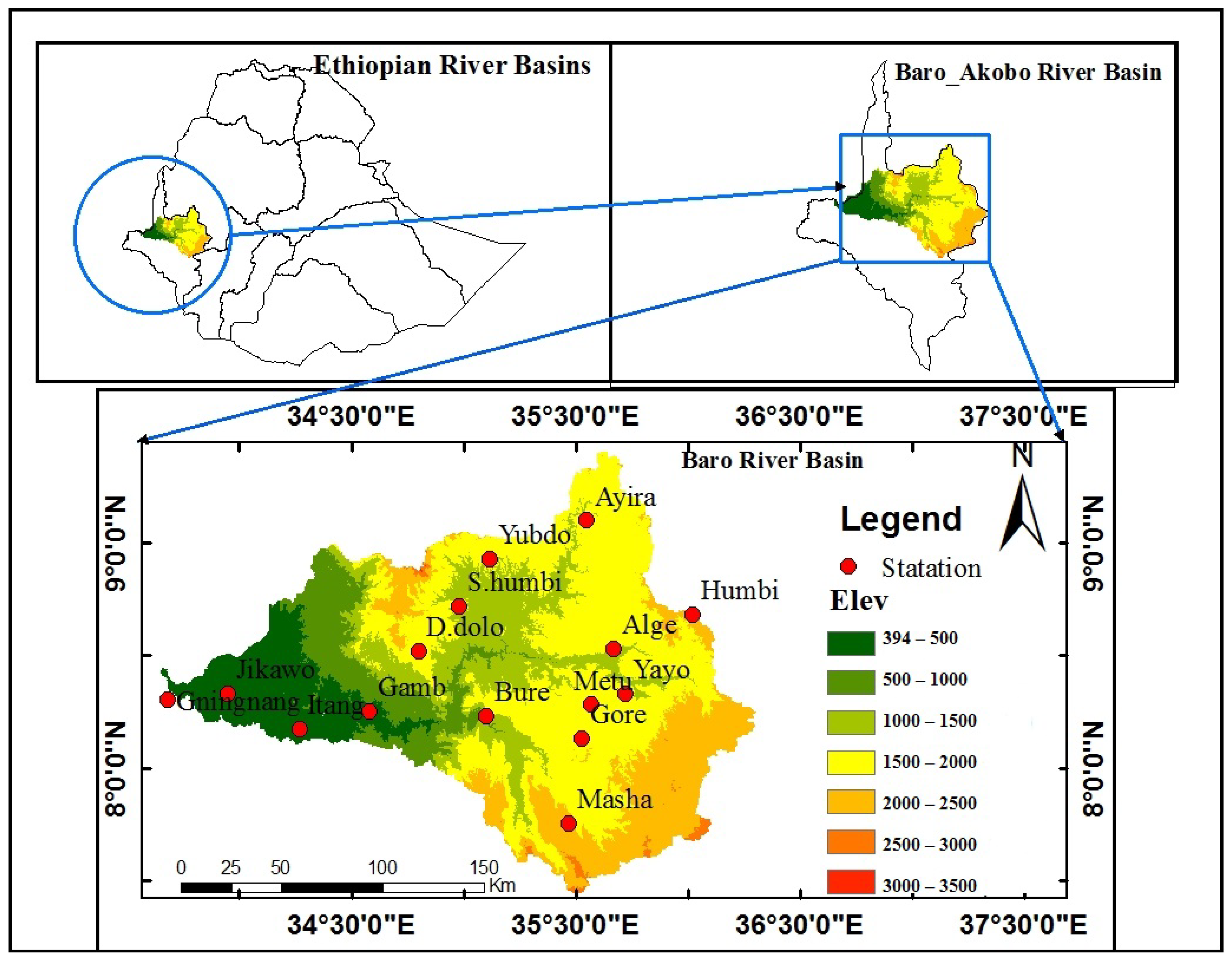
The Baro basin is located in southwest Ethiopia, between the latitudes of 7°24′ and 9°25′ and longitudes of 33°20′ and 36°20′, and spans over 23,000 km2 (Figure 1). The Baro River was created by the confluence of the Birbir and Geba rivers east of Metu in the Oromia region’s Ilu Aba Bora Zone, and it is the greatest tributary, accounting for 83% of the total water flowing into the Sobat River, which is connected to the White Nile in South Sudan. During the rainy season from June to October, the Baro River alone supplies around 14% of Nile water [17].
The basin’s elevation ranges from 3500 m above sea level in the eastern highlands to less than 400 m in the Gambella plain. The eastern part of the basin consists of the hilly upland and falls steeply to the lower plain of the Gambella Region. Due to its wide variations in elevation, there is a significant difference in temperature in the basin, with the maximum and minimum temperatures ranging from 17.7 to 42 °C and 6.4 to 27 °C, respectively [18]. The area shows a mono-modal rainfall pattern, with a single rainfall peak, and from less than 1000 mm in the lower Baro to over 2500 mm. There are two distinct seasons: Bega season (November, December, January, and February) and Kiremt season (May to October) [19].
2.2. Data Sources, Collection, and Analysis
2.2.1. Meteorological Data
Daily meteorological and gridded data for the basin’s selected stations were obtained from the Ethiopian National Meteorological Agency (ENMA) from 2001 to 2018. Those stations were chosen according to their longitudinal representativeness of the basin from upstream to downstream, as well as their basin coverage (Table 1). The first stage of this research was data quality control, which included analyzing the data availability, screening for outliers, performing a homogeneity test, and then filling in the missing data.
The total data availability as a percentage for 18 years from 2001 to 2018 was analyzed. The number of years was fixed based on the fullness of the observed data, and then annual numbers of non-missing values were estimated for each of the stations. Some stations, such as Masha in 2016, Itang in 2015 and 2018, Alge in 2011, Bure in 2008 and 2011, Dembidolo from 2008 to 2011, and Humbi in 2017, have entire years of missing data. It was decided in this scenario to merge those stations with satellite data, where Chirps was chosen in this study. Again, for those stations where the location was important for this study and there were insufficient data, data was extracted from Ethiopian National Meteorological Agency’s (ENMA) NetCDF gridded data. Some researchers found that merging observed station data with satellite rainfall data produced a better estimate than any of the original data [20,21].
The outlier test was applied to the station data, taking into account the target station’s elevation as well as that of nearby stations. The maximum precipitation limit for each station was set to 100 by studying historical data from the station, although at least four neighbors were reviewed for comparison before the outlier was removed. The missing value for the rainfall record outlier was then filled using the inverse distance method. Outlier test findings that were isolated and had significant variances above the mean value of the surrounding stations were also considered suspicious and cross-checked in the analysis. After taking into account all of these criteria, the outliers for each month were examined.
A homogeneity test was also performed for all of the stations in the basin, and the Pettit test was used to detect changes in the data. Homogeneity tests were used to determine whether or not a climate time series was homogeneous over time [22]. Quantile matching was used to adjust some data sets that were not homogeneous [23]. The inverse distance weightage (IDW) approach, which was integrated into the climate data tool, was used to fill in missing data. A minimum of three surrounding stations were used for spatial interpolation. The interpolated data had a direct link with the number of surrounding stations examined for interpolation.
On ArcGIS, the average precipitation over the basin was calculated using the Thiessen polygon method. From the result, it was found that the basin’s average precipitation was 1555 mm. Moreover, thirty years of data showed that the annual rainfall in the basin lies between 300 mm in the lowland and 2500 mm in the highland part of the basin. The Baro river basin receives the maximum monthly rainfall in August and the least in January, but there is no consistent pattern found temporally.
2.2.2. Land Use/Land Cover and Topographic Dataset
The land use and land cover change analysis for the Baro river basin was assessed using the Google Earth Engine cloud computing platform (https://code.earthengine.google.com/ (accessed on 15 June 2022)). Google Earth Engine (GEE) makes the land use and land cover change analysis more manageable, increasing the efficiency and involving less time [24]. An image composition of Landsat 5, 7, and 8 tier 1 TOA reflectance was applied in this analysis. In addition, the forest loss change trend in the basin was estimated using Hansen Global Forest Change v. 1.9 (2000–2021) on the Google Earth Engine cloud computing platform (https://developers.google.com/earth-engine/datasets/catalog/UMD_hansen_global_forest_change_2021_v1_9; (accessed on 12 June 2022)).
The elevation of the earth’s surface in relation to a reference datum was represented digitally by a digital elevation model (DEM). Terrain attributes such as elevation were determined using the DEM in this study for the processing of hydrological and meteorological station locations and watershed outlines on ArcGIS software.
2.2.3. Catchment Dataset
In the upland areas of the basin, 11 catchments of varying sizes ranging from 36 to 7940 km2 were chosen. The catchments were identified in an area where it was assumed that there was homogeneity between them, so that the catchment size would be the only factor taken into consideration for the analysis. This reduced the impact of other catchment characteristics in our analysis, such as land use, land cover, topography, antecedent moisture conditions, and other climatological impacts.
2.3. Methodology
2.3.1. Statistical Analysis
This study used the Climate Data Tool (CDT) version 7.0, R programming, Python, and STATA for the statistical analyses of the meteorological data for the study area. CDT is an open-source R-based program with a simple graphical user interface for analyzing meteorological data. CDT’s main functionalities include station data organization, quality control, and processing; downloading and processing of various satellite rainfall estimates and the reanalysis of data; merging station observations with proxies (satellite rainfall estimates and the reanalysis of temperature products); data extraction from gridded products at any point, for any selected box, and for any administrative boundary; and various analyses and visualizations of stations and gridded data [22,25,26]. The CDT tool was created with the aim of bridging the critical gaps in climate services and applications, particularly in Africa [27,28], which happens due to a challenge in the availability and access of climate data.
2.3.2. Land Use/Cover Change Analysis
Top-of-atmosphere (TOA) reflectance products from Landsat-5 Thematic Mapper (TM), Landsat-7 Enhanced Thematic Mapper Plus (ETM+), and Landsat-8 Operational Land Imager (OLI) were used for land cover change analyses (available online: https://code.earthengine.google.com/ (accessed on 15 June 2022)). Following that, the Landsat datasets covering the study area were imported as image collections into Google Earth Engine (GEE), a cloud-based geospatial analysis tool, for further preprocessing activities.
For land use/cover classification, the random forest (RF) classifier was used. It was trained using 70% of the training data sets that were randomly chosen, and the remaining 30% were used for model validation. RF was chosen because, in comparison to other classifiers, it produces a higher classification accuracy, needs less model training time, and is less sensitive to training samples. Finally, the validation accuracy and kappa accuracy on GEE were used to evaluate the classification model’s overall performance. To understand specifically the relationship between forest change and meteorological variability, the annual forest loss trend for the basin and sub-basin was estimated using the Hansen Global Forest Change v1.9 (2000–2021) (available online: https://developers.google.com/earth-engine/datasets/catalog/UMD_hansen_global_forest_change_2021_v1_9; accessed on 12 June 2022)). The land use/cover change between the periods of 2000, 2018, and 2022 was also estimated on GEE using the following calculations for estimating the LULC change rate:
where R is the LULC change rate, Lt is the land cover type in year t, Lt−1 is the land cover in the most recent time interval, and is the time interval.
2.3.3. Sensitivity Analysis
We used the Pearson correlation coefficient to evaluate the sensitivity of the precipitation and temperature variability to changes in land use/cover, elevation, and catchment size. The Pearson coefficient is known as the best approach for measuring the relationship between variables of interest, as it is based on the method of covariance [29]. It indicates the magnitude of the correlation as well as the direction of the relationship:
where r is the correlation coefficient, n is the number in the given dataset, x is the first variable in the context, and y is the second variable.
3. Results and Discussions
3.1. Relationship between Variability in Rainfall and Topography
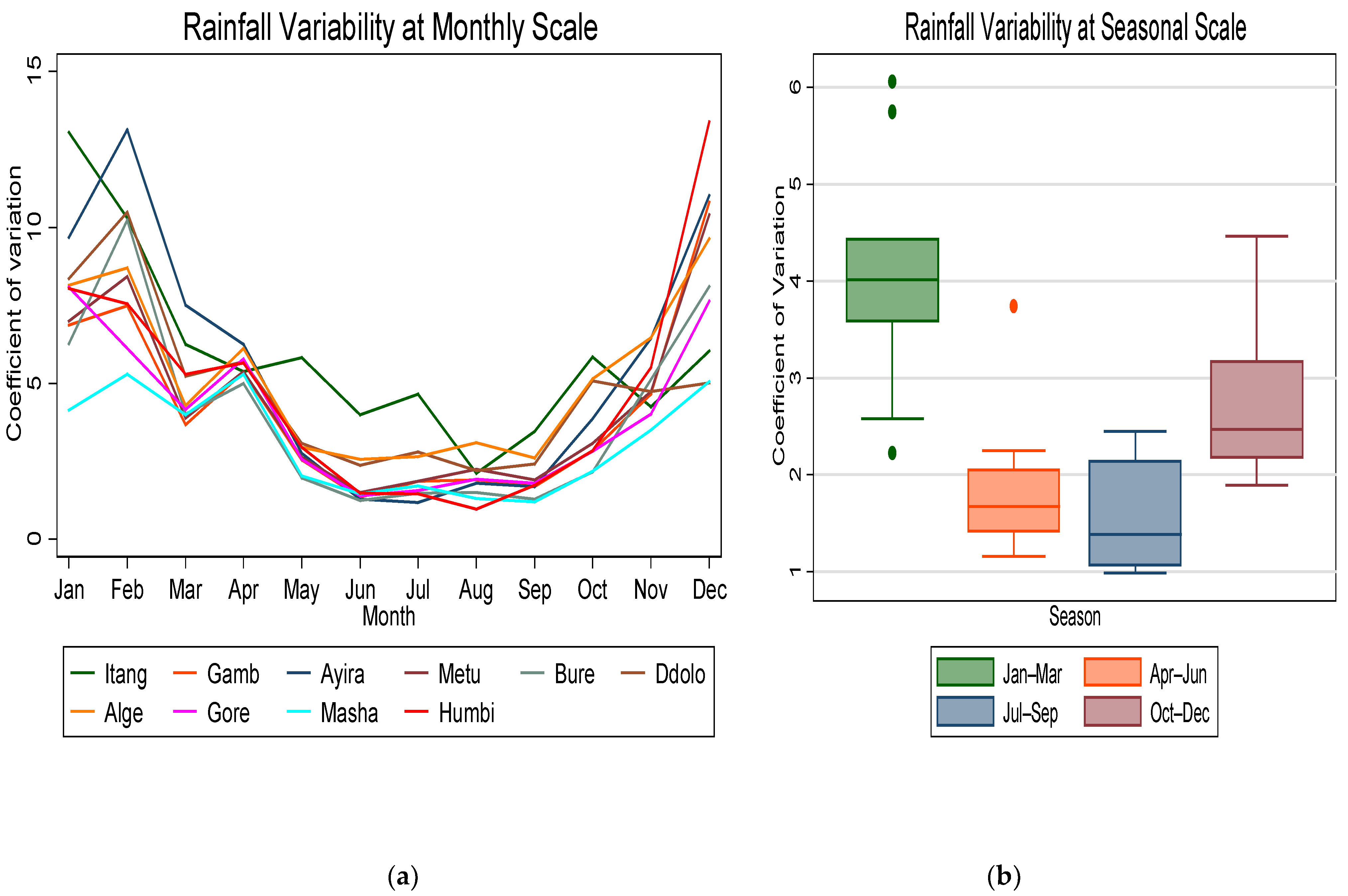
The temporal variability in rainfall in the basin was estimated and compared spatially throughout the basin. The graph below shows that the rainfall variability was highest (Figure 2a) during the dry season, dropped during the Kiremt season, and then rose again starting in September. The highest coefficient of variation (CV) value was noticed in January (13.04), where it decreased to July and August (1.17) and where the minimum value was found. Comparing the variability before and after interpolation, it was found that rainfall data after interpolation has the lowest coefficient of variation (from 0.62 to 3.01), which might have been caused by the interpolation factor. The coefficient of variation value estimated from the observed data prior to interpolation and the observed data merged with the satellite data, on the other hand, gave almost identical estimates for the two variables (from 1.17 to 13.04). Therefore, it is vital to either estimate the variability using observed data prior to interpolation or to use merged rainfall data with satellite data in order to reduce the uncertainty that may occur in the estimation of rainfall variability due to the interpolation of the missing data.
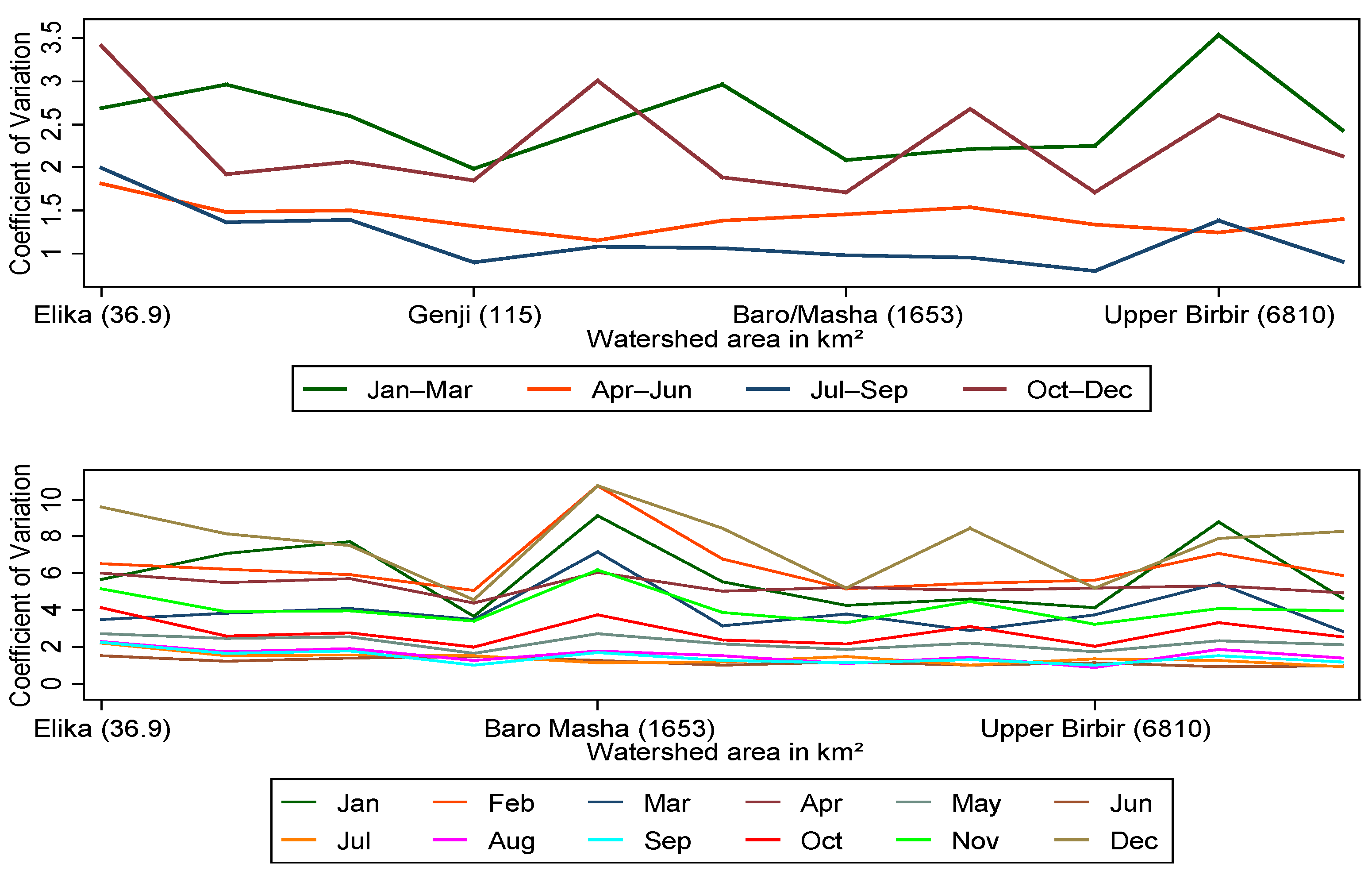
The rainfall variability was also estimated at the seasonal scale, as shown in the figure below (Figure 2b), and it was found that the maximum variation was calculated in the dry season from January to March (5.76), which decreased down in the Kiremt season (1.04). Then, starting from the fourth season (October to December), the trend started to rise again. Overall, regardless of the catchment spatial variability, the temporal variability both at the monthly and seasonal scales of rainfall followed a similar pattern. For all stations, the highest variability in rainfall occurred in January, when it fell during the Kiremt season and then rose again. The graph below (Figure 2) shows the patterns of the spatiotemporal variability in rainfall for selected stations in the basin.
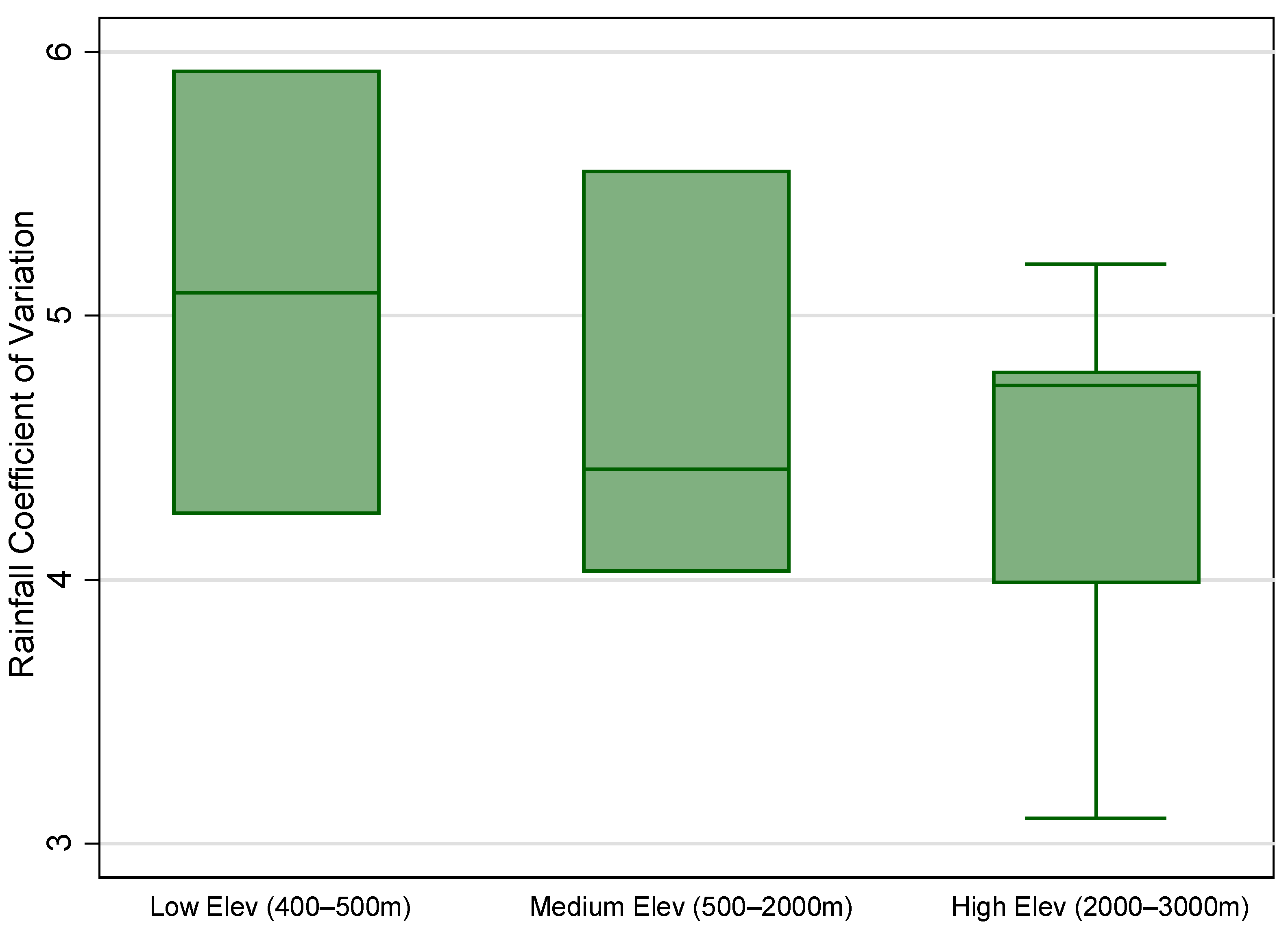
We divided the elevation difference into three groups, lower elevation (400–500 m), medium elevation (500–2000 m), and higher elevation (2000 and above), to clearly show the relationship between rainfall variability and the topographical variation in the study area. Then, a boxplot was developed as shown in Figure 3 below.
As can be seen from Figure 3, the variability in rainfall showed a decrease in the basin with a rise in elevation. The results of this study support the findings of Pendergrass et al., 2017 [30] that climate warming increases rainfall variability. Figure 2a also shows that Itang, the basin’s lowest station at an elevation of 415 m above mean sea level (amsl), had a larger coefficient of variation value (13.01) in January. Furthermore, this figure shows that the precipitation variability was generally stronger at shorter time scales, with the monthly variability being greater than the seasonal variability, for example (see Figure 2a). This result agrees with those reported in [31], the authors of which came to the conclusion that rainfall variability is higher at shorter time scales. Recent studies also show that future global and regional warming increase precipitation variability over a range of time scales [32,33,34].
3.2. Relationship between Variability in Temperature and Topography
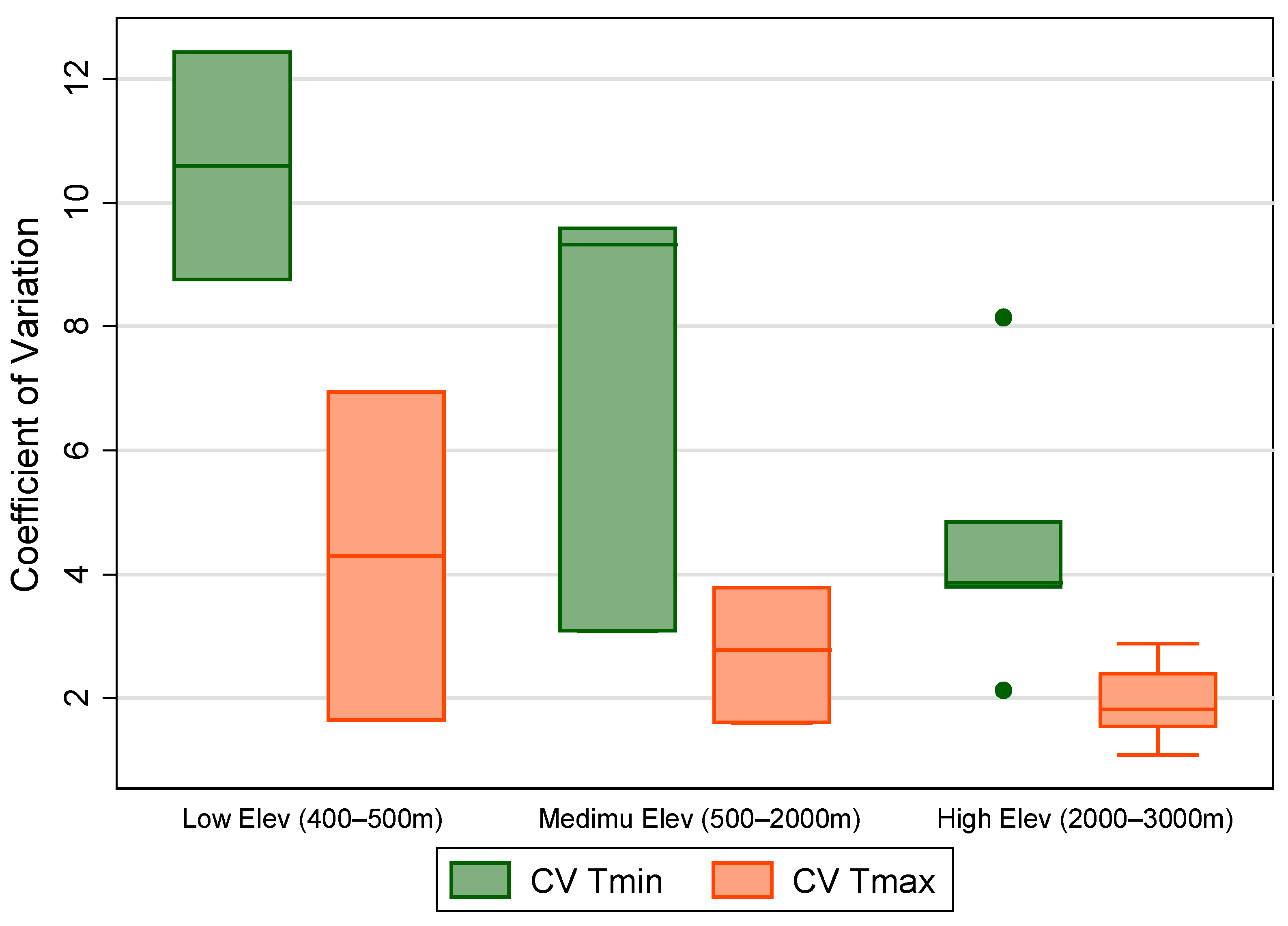
Temperature variation in the basin was also examined to determine its relationship to elevation variation. The elevation of the basin was divided into three categories for this analysis: 400–500 m as low elevation, 500–2000 m as medium elevation, and 2000–3000 m and above as high elevation. Then, we drew a graph to illustrate the relationship between the two, and it was observed that as elevation increased, the variability in the maximum and minimum temperatures decreased (see Figure 4). On the other hand, we observed that the minimum temperature variability was greater (with a coefficient of variation of 12.4 in the lower elevation and 2.6 in the higher elevation) than the maximum temperature variability (with a coefficient of variation of 6.5 in the lower elevation and 1.5 in the higher elevation).
3.3. Relationship between Variability in Rainfall and Catchment Scale
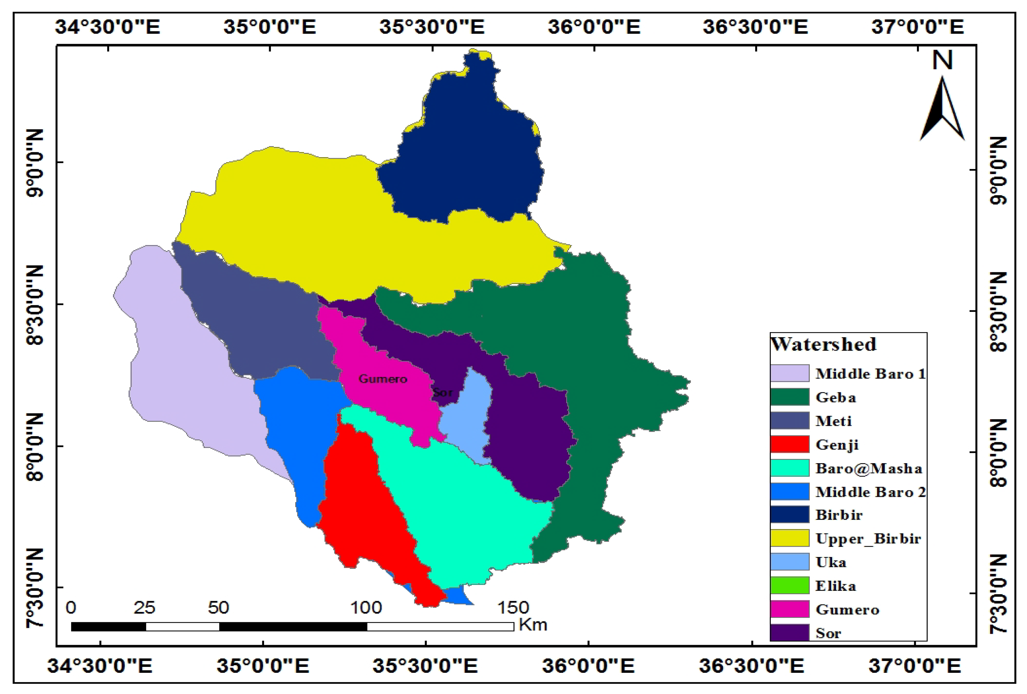
The upper Baro catchment’s watersheds of varying sizes were chosen to explore the relationship between catchment size and rainfall variability. Watersheds were chosen in areas where other variables such as climate and the land use and land cover distribution were expected to be homogeneous in order to minimize their impact on our analysis. As a result, 11 watersheds ranging in size from 36 to 7940 km2 were chosen in the upper Baro, where climatological and land use/cover homogeneity was expected. The areal precipitation for each watershed was then estimated using the Thiessen polygon method. Finally, the average coefficient of variation for each watershed was calculated seasonally and monthly to see if there was a relationship between rainfall variability and catchment size. The map below (see Figure 5) shows the basin’s selected watersheds for this analysis.
The coefficient of variation for each season was used to calculate the rainfall variability in those watersheds, but no clear relationship between rainfall variability and catchment size was found (see Figure 6 below). This finding supports the conclusions reached by the authors of [8,35], who concluded that there was no significant relationship found between precipitation and catchment size based on their analysis. This study goes beyond that, attempting to determine whether the meteorological variability was linked to catchment size; however, no significant relationship was discovered between the two.
3.4. Relationship between the Variability in Meteorological Variables and Land Use/Cover Change
Due to the high population density in the region, the land use/cover of the Baro basin is continually changing [36,37]. According to research conducted in the area, in the Ilu Aba Bora Zone, which contributes to the majority of the Baro basin, 80% of the new agricultural land was converted from forests [38]. For estimating the forest loss change trends in the basin, a time series of annual forest loss was extracted using Google Earth Engine from Hansen Global Forest Change v. 1.9 (2000–2021) (https://developers.google.com/earth-engine/datasets/catalog/UMD_hansen_global_forest_change_2021_v1_9; (accessed on 12 July 2022)). The Hansen global forest change dataset characterizes the forest extent and changes worldwide from 2000 to 2021 using a time-series analysis of high-resolution (30 m) Landsat images. The authors of [39,40] found that the Hansen dataset was effective for performing land cover analyses at the local government level in their studies.
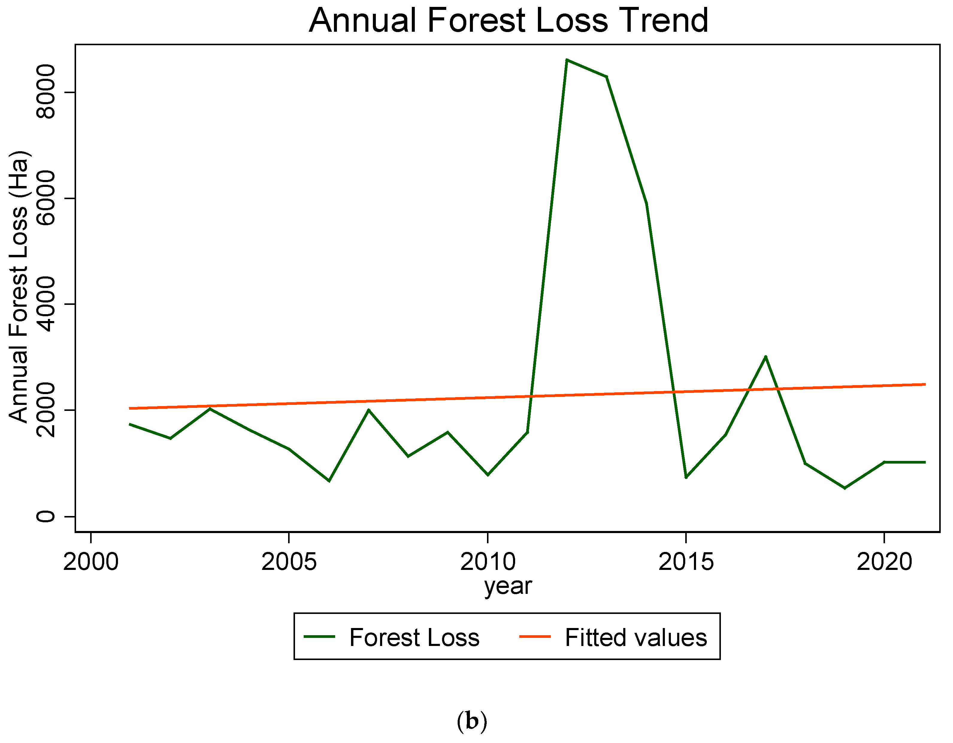
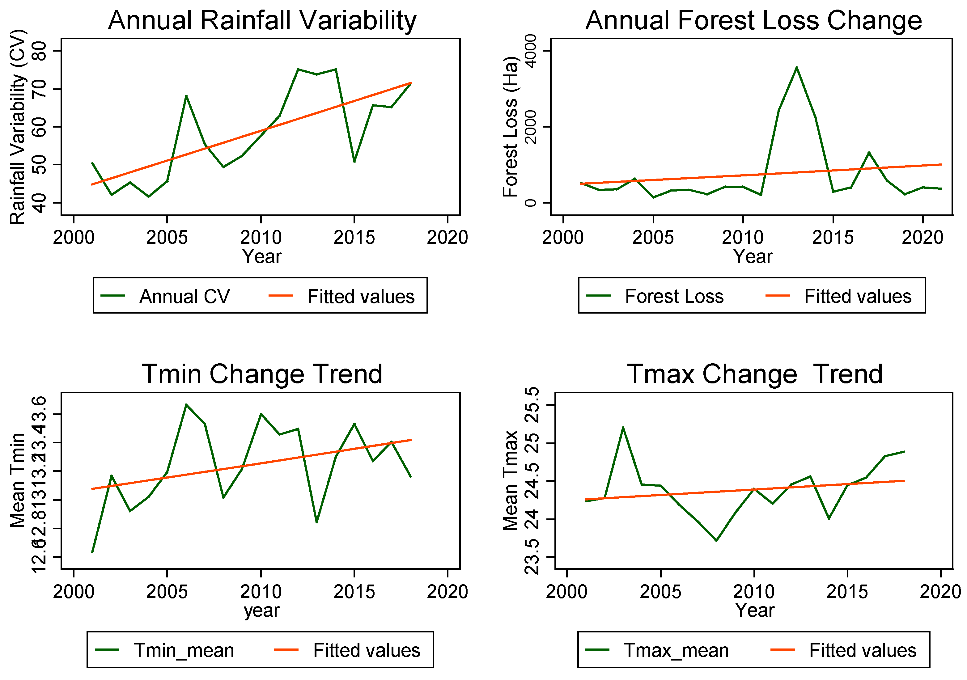
Using the Hansen dataset, it was found that the largest annual forest losses in the Baro river basin happened in 2012, 2013, and 2014, with losses of 8605ha, 8289ha, and 5895ha, respectively, and with an increasing cumulative trend from 2001 to 2021. As a result, the basin lost an average of 2265.04 ha per year, as shown in Figure 7a,b. These data are consistent with the findings of the Global Forest Watch, which conducted a continuous study on Ethiopian deforestation rates and statistics from 2000 to 2021 (https://www.globalforestwatch.org/dashboards/country/ETH; accessed on 8 October 2022).
NDVI imagery was also developed and estimated for the Baro river basin using Landsat 7 and 8 Collection 1 Tier 1 8-Day NDVI Composite, as shown in Figure 8 below, and the NDVI showed an increasing trend with a range of 0.083. However, this does not necessarily imply that open and dense forests are expanding; rather, it means that negligible areas are being converted to bare land. As the authors of [31] indicated, NDVI values between 0.2 and 0.5 indicate sparse vegetation such as shrubs and grasslands, and NDVI values between 0.6 and 0.9 suggest dense forest.
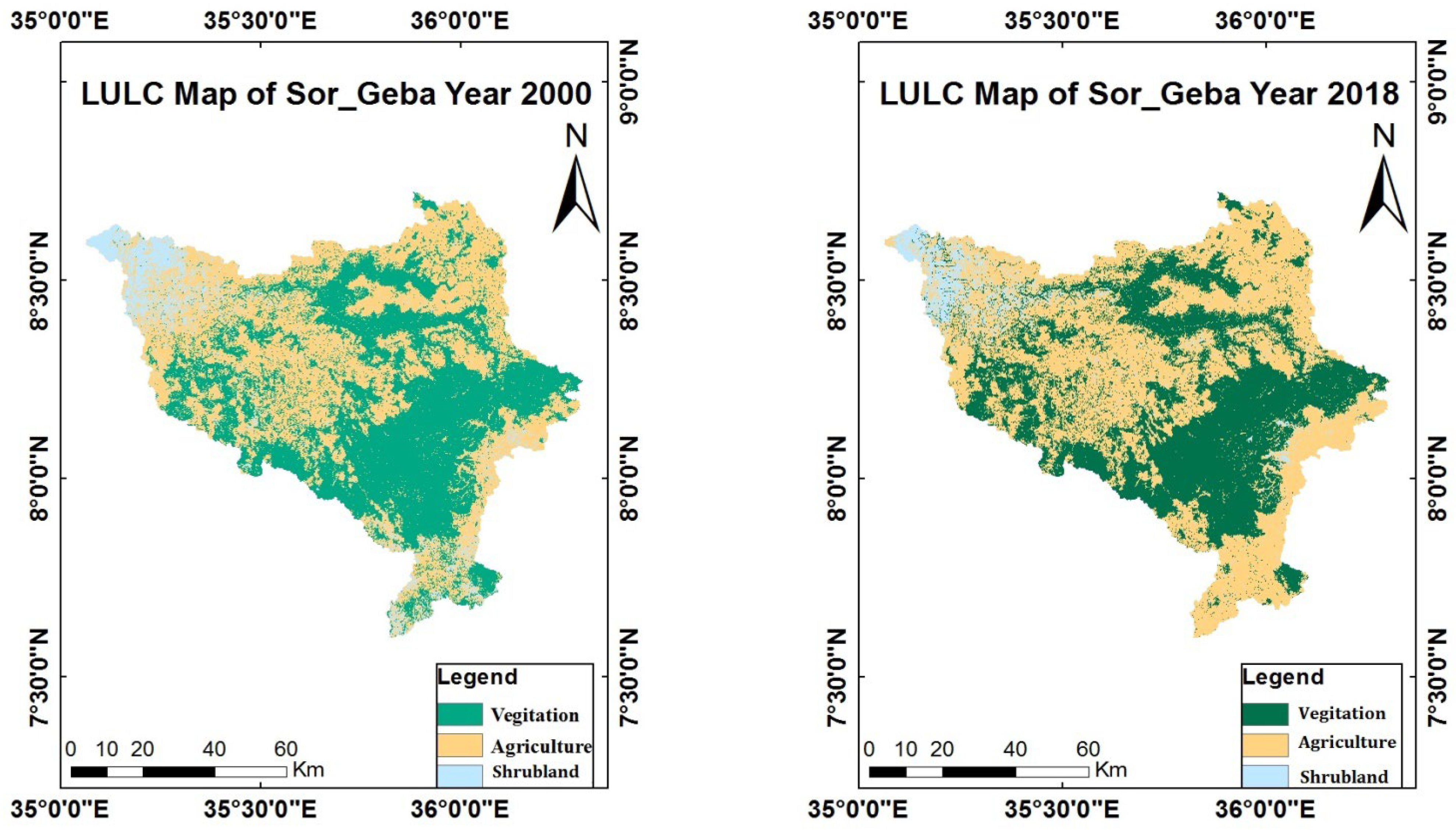
On the other hand, to examine the relationship between rainfall variability and land use/cover changes, the LULC change was estimated for the Sor_Geba catchment, which is located in the upper part of the basin. This catchment was chosen because it is a homogeneous area with consistent climatic and topographic conditions, enabling us to concentrate exclusively on the influence of landcover changes on meteorological variability. The land use/cover change between 2000 and 2018 was determined using Google Earth Engine. According to the findings, between 2000 and 2018, the forest cover decreased from 3656 km2 to 3287 km2, whereas the agricultural land increased from 3653 km2 to 4169 km2. Moreover, shrubland showed a pattern of decrease from 611 km2 to 463 km2 (see Figure 9).
The Hansen global forest change estimates were also used to evaluate the trend in forest degradation for the Sor_Geba catchment, and the years 2012, 2013, and 2014 show an annual maximum loss of 2434, 3568, and 2261 ha, respectively. This equates to an estimated average annual loss of 821.63 hectares in the watershed, with a total increasing trend from 2001 to 2018 and a range of 3241 ha. The results of the analysis are consistent with previous research [41] and the authors of [42] who looked at the overall land use/cover changes in the catchment.
In general, when forest degradation increased in the basin, both rainfall and temperature variability showed an increasing trend. Figure 10 shows that the variability in the maximum temperature, minimum temperature, and rainfall is increasing, indicating that they have a positive correlation with forest loss. This study is supported by the findings of Buba et al., 2020 [43], who looked into the relationship between forest degradation and climate variability in Nigeria. Their evaluation found a positive relationship between forest loss and climate variability (temperature and rainfall variability), with a correlation of 0.58.
3.5. Correlation of Catchment Size, Topography, and Land Use/Cover with Precipitation and Temperature Variability
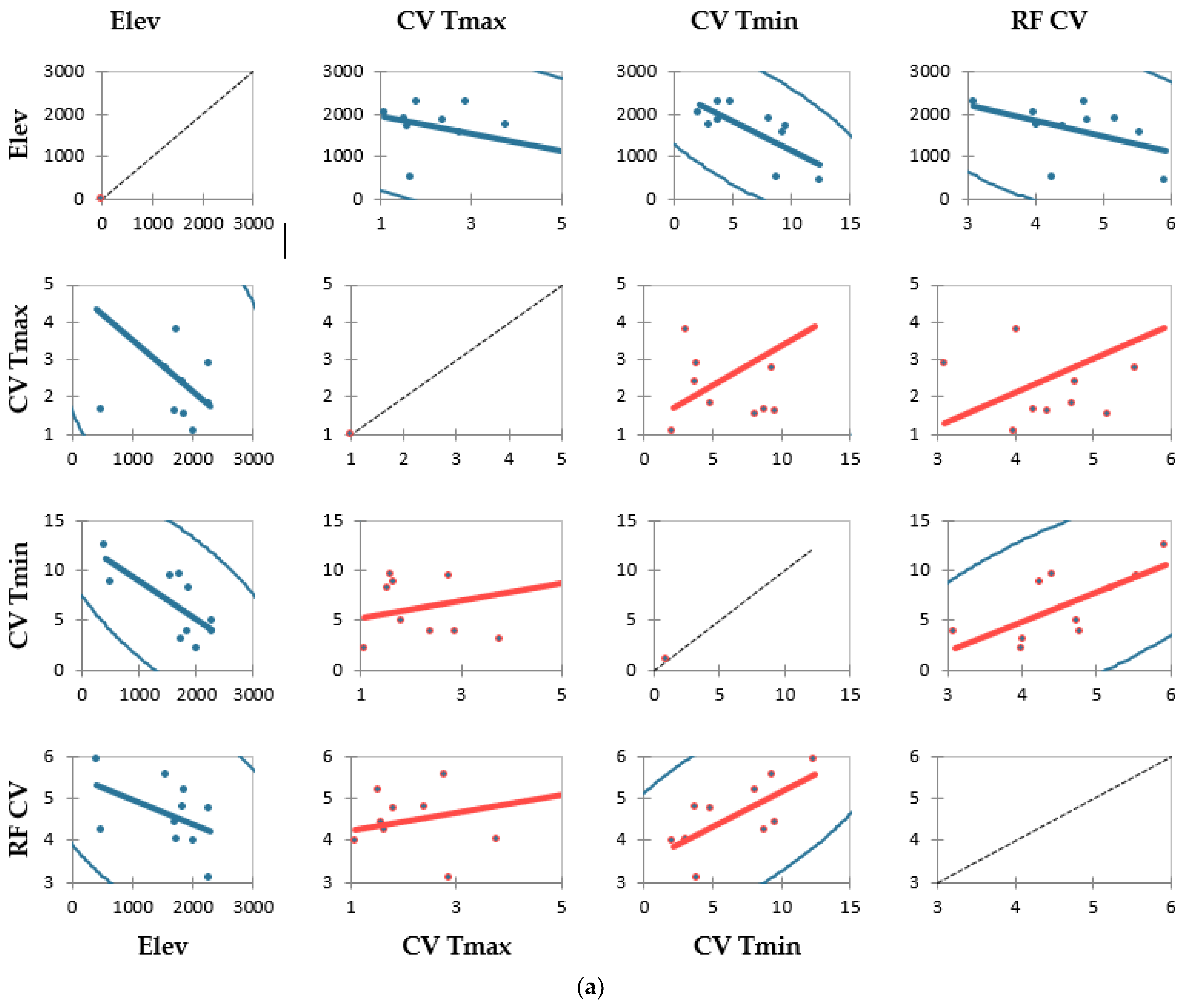
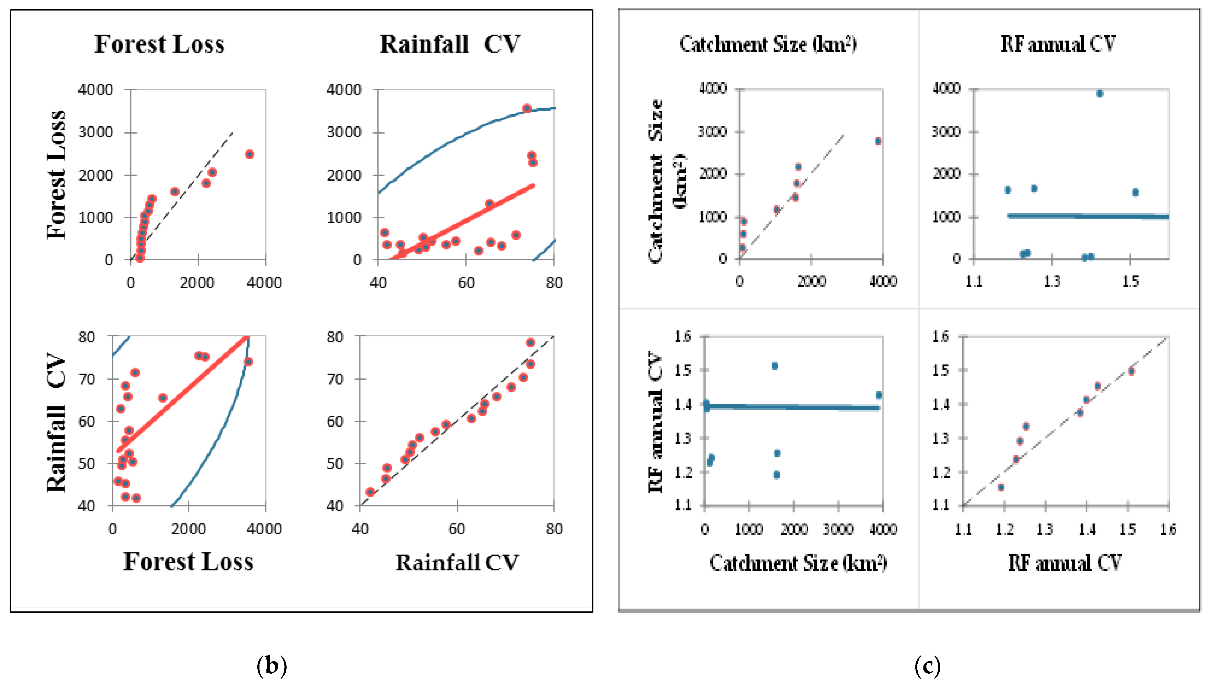
A correlation analysis was carried out to determine which catchment characteristics have the greatest influence on the variability in precipitation and temperature. First, by ranking the area from small (36 km2) to large (7940 km2), the relationship between catchment size and precipitation variability was examined. A correlation of −0.13 was found, indicating a negligible relationship between the two (Figure 11c, Figure 12c and Table 2c).
As shown in Table 2a, the relationship between elevation, rainfall, and temperature variability was also investigated. The Pearson correlation between rainfall variability with elevation, maximum temperature variability with elevation, and minimum temperature variability with elevation was estimated in the analysis and found to be −0.47, −0.72, and −0.53, respectively, with a negative sign indicating an inverse relationship between the two.
Furthermore, for the years 2001 to 2018, a correlation was determined to investigate the relationship between land cover change (represented by forest, which is the main landcover type in the area) and rainfall variability (Table 2b). As a result, a 0.65 correlation with a positive relationship was observed between forest loss and rainfall variability.
Generally, it was found that land use/cover changes and elevation variation were the two most influential factors for the variability in meteorological variables.
4. Conclusions
Several studies have been conducted to assess the impact of climate change and land use/cover change on hydrological processes and catchment characteristics. However, in reverse, the impact of those catchment characteristics on meteorological variable dynamics remains limited. The sensitivity of meteorological variable dynamics to variations in catchment characteristics was investigated in this study, focusing on three catchment characteristics: catchment size, elevation (topographical difference), and land use/cover changes.
Statistical tools were used to assess the variability in rainfall and temperature with these catchment characteristics. Climate data tools, R programming, and STATA were used to assess the variability in rainfall and temperature, while Google Earth Engine was used to assess the changes in land use/cover. After selecting meteorological stations and arranging them longitudinally along river basins, a correlation was developed between elevation changes and the variability in rainfall and temperature.
Watersheds from the basin were selected to study the relationship between catchment size and rainfall variability. Those watersheds were chosen in a region where the climatological and catchment characteristics were assumed to be homogeneous in order to minimize their effects on the analysis of this special topic. The catchment sizes were then arranged from small (36 km2) to large (7940 km2) for a specific time period, and a correlation with rainfall variability was estimated. As a result, no significant relationship between the two was found.
A correlation was also checked between land use/cover changes with precipitation and temperature variability. We found a good correlation between rainfall variability and land use/cover changes (0.65) compared to the correlation between land use/cover changes and temperature variability.
In general, we observed that land use/cover changes had the greatest influence on precipitation variability, followed by elevation variation, whereas elevation variation has the greatest influence on temperature variability. However, no correlation was found between catchment size and precipitation variability. More research is needed to assess the effect of catchment size on meteorological variability, taking into account all other characteristics within the watersheds. It is also desirable to make decisions using full meteorological data rather than filled data, and considerations such as the impact of areal averaging must also be considered.
Only two meteorological variables, precipitation and temperature, were used for the analysis of meteorological variable dynamics in this study, but we urge that future researchers consider other variables, such as wind and humidity, in their analyses. We also recommend more research into such issues, taking into account the impact of combined and relative effects in order to draw a conclusion about the overall sensitivity of meteorological dynamics to changes in catchment characteristics.
Author Contributions
S.M.K., conceptualized the study, conducted data analyses, and wrote the manuscript; T.T., framed the design and participated in review, editing, and supervision; G.T., conceptualized the study, participated in review and editing, and formatted the analyses; and K.E.T., provided software. All authors have read and agreed to the published version of the manuscript.
Funding
This research received no external funding.
Institutional Review Board Statement
Not applicable.
Institutional Consent Statement
Not applicable.
Data Availability Statement
All data models and code generated or used during the paper can be found in the submitted article.
Acknowledgments
This research was financially supported by the Africa Center of Excellence for Water Management (ACEWM) hosted by Addis Ababa University. The authors acknowledge the National Meteorological Agency (NMA) for providing the relevant data.
Conflicts of Interest
The authors declare no conflict of interest.
References
- Patel, A.; Goswami, A.; Dharpure, J.K.; Thamban, M. Rainfall Variability over the Indus, Ganga, and Brahmaputra River Basins: A Spatio-Temporal Characterisation. Quat. Int. 2021, 575–576, 280–294. [Google Scholar] [CrossRef]
- Ringard, J.; Chiriaco, M.; Bastin, S.; Habets, F. Recent Trends in Climate Variability at the Local Scale Using 40 Years of Observations: The Case of the Paris Region of France. Atmos. Chem. Phys. 2019, 19, 13129–13155. [Google Scholar] [CrossRef] [Green Version]
- Tan, X.; Wu, Y.; Liu, B.; Chen, S. Inconsistent Changes in Global Precipitation Seasonality in Seven Precipitation Datasets. Clim. Dyn. 2020, 54, 3091–3108. [Google Scholar] [CrossRef]
- Guntu, R.K.; Agarwal, A. Investigation of Precipitation Variability and Extremes Using Information Theory. Environ. Sci. Proc. 2021, 4, 14. [Google Scholar] [CrossRef]
- Liu, L.; Zhang, X. Effects of Temperature Variability and Extremes on Spring Phenology across the Contiguous United States from 1982 to 2016. Sci. Rep. 2020, 10, 17952. [Google Scholar] [CrossRef]
- Li, J.; Zheng, X.; Zhang, C.; Chen, Y. Impact of Land-Use and Land-Cover Change on Meteorology in the Beijing–Tianjin–Hebei Region from 1990 to 2010. Sustainability 2018, 10, 176. [Google Scholar] [CrossRef] [Green Version]
- Deng, Y.; Wang, S.; Bai, X.; Tian, Y.; Wu, L.; Xiao, J.; Chen, F.; Qian, Q. Relationship among Land Surface Temperature and LUCC, NDVI in Typical Karst Area. Sci. Rep. 2018, 8, 64. [Google Scholar] [CrossRef] [Green Version]
- Wang, H.; Xuan, Y. Spatial Variation of Catchment-Oriented Extreme Rainfall in England and Wales. Atmos. Res. 2022, 266, 105968. [Google Scholar] [CrossRef]
- Sanchez-Moreno, J.F.; Mannaerts, C.M.; Jetten, V. Influence of Topography on Rainfall Variability in Santiago Island, Cape Verde. Int. J. Clim. 2014, 34, 1081–1097. [Google Scholar] [CrossRef]
- Chu, X.L.; Lu, Z.; Wei, D.; Lei, G.P. Effects of Land Use/Cover Change (LUCC) on the Spatiotemporal Variability of Precipitation and Temperature in the Songnen Plain, China. J. Integr. Agric. 2022, 21, 235–248. [Google Scholar] [CrossRef]
- Mora, B.; Herold, M. Land Cover and Change. GOFC-GOLD L. Cover Proj. Off. Newsl. 2015, II, 1–6. [Google Scholar]
- Isabirye, M.; Raju, D.V.; Kitutu, M.; Yemeline, V.; Deckers, J.; Poesen, J. Sugarcane Biomass Production and Renewable Energy; IntechOpen: London, UK, 2013. [Google Scholar]
- Shao, J.; Li, Y.; Ni, J. The Characteristics of Temperature Variability with Terrain, Latitude and Longitude in Sichuan-Chongqing Region. J. Geogr. Sci. 2012, 22, 223–244. [Google Scholar] [CrossRef]
- Aher, S.; Shinde, S.; Gawali, P.; Deshmukh, P.; Venkata, L.B. Spatio-Temporal Analysis and Estimation of Rainfall Variability in and around Upper Godavari River Basin, India. Arab. J. Geosci. 2019, 12, 682. [Google Scholar] [CrossRef]
- Lv, X.; Zuo, Z.; Ni, Y.; Sun, J.; Wang, H. The Effects of Climate and Catchment Characteristic Change on Streamflow in a Typical Tributary of the Yellow River. Sci. Rep. 2019, 9, 14535. [Google Scholar] [CrossRef] [Green Version]
- Köplin, N.; Viviroli, D.; Schadler, B.; Weingartner, R. How Catchment Characteristics Determine Hydrological Sensitivity to Climate Change in a Mountainous Environment. Geophys. Res. Abstr. 2010, 12, 3487. [Google Scholar] [CrossRef]
- Kassa, T. Assessment of Groundwater Potential Zones in Baro Basin Using GIS and Remote Sensing. Master’s Degree, Arba Minch University, Arba Minch, Ethiopia, 2015. [Google Scholar] [CrossRef]
- Kebede, A. An Assessment of Temperature and Precipitation Change Projections Using a Regional and a Global Climate Model for the Baro-Akobo Basin, Nile Basin, Ethiopia. J. Earth Sci. Clim. Chang. 2013, 4, 1–12. [Google Scholar] [CrossRef]
- Alemayehu, T.; Kebede, S.; Liu, L.; Kebede, T. Basin Hydrogeological Characterization Using Remote Sensing, Hydrogeochemical and Isotope Methods (the Case of Baro-Akobo, Eastern Nile, Ethiopia). Environ. Earth Sci. 2017, 76, 466. [Google Scholar] [CrossRef]
- Hu, Q.; Li, Z.; Wang, L.; Huang, Y.; Wang, Y.; Li, L. Rainfall Spatial Estimations: A Review from Spatial Interpolation to Multi-Source Data Merging. Water 2019, 11, 579. [Google Scholar] [CrossRef] [Green Version]
- Tadesse, K.E.; Melesse, A.M.; Abebe, A.; Lakew, H.B.; Paron, P. Evaluation of Global Precipitation Products over Wabi Shebelle River Basin, Ethiopia. Hydrology 2022, 9, 66. [Google Scholar] [CrossRef]
- Dinku, T.; Faniriantsoa, R.; Islam, S.; Nsengiyumva, G. The Climate Data Tool: Enhancing Climate Services Across Africa. Front. Clim. 2022, 3, 1–16. [Google Scholar] [CrossRef]
- Squintu, A.A.; van der Schrier, G.; Brugnara, Y.; Klein Tank, A. Homogenization of Daily ECA & amp; D Temperature Series. Int. J. Climatol. 2019, 39, 1243–1261. [Google Scholar] [CrossRef] [Green Version]
- Noi Phan, T.; Kuch, V.; Lehnert, L.W. Land Cover Classification Using Google Earth Engine and Random Forest Classifier-the Role of Image Composition. Remote Sens. 2020, 12, 2411. [Google Scholar] [CrossRef]
- Dinku, T.; Thomson, M.C.; Cousin, R.; del Corral, J.; Ceccato, P.; Hansen, J.; Connor, S.J. Enhancing National Climate Services (ENACTS) for Development in Africa. Clim. Dev. 2018, 10, 664–672. [Google Scholar] [CrossRef]
- Grossi, A.; Dinku, T. Enhancing National Climate Services: How Systems Thinking Can Accelerate Locally Led Adaptation. One Earth 2022, 5, 74–83. [Google Scholar] [CrossRef]
- Dinku, T.; Block, P.; Sharoff, J.; Hailemariam, K.; Osgood, D.; del Corral, J.; Cousin, R.; Thomson, M.C. Bridging Critical Gaps in Climate Services and Applications in Africa. Earth Perspect. 2014, 1, 15. [Google Scholar] [CrossRef] [Green Version]
- Dinku, T. Challenges with Availability and Quality of Climate Data in Africa; Elsevier Inc.: Amsterdam, The Netherlands, 2019; ISBN 9780128159989. [Google Scholar]
- Meng, M.; Huang, N.; Wu, M.; Pei, J.; Wang, J.; Niu, Z. Vegetation Change in Response to Climate Factors and Human Activities on the Mongolian Plateau. PeerJ 2019, 7, e7735. [Google Scholar] [CrossRef]
- Pendergrass, A.G.; Knutti, R.; Lehner, F.; Deser, C.; Sanderson, B.M. Precipitation Variability Increases in a Warmer Climate. Sci. Rep. 2017, 7, 17966. [Google Scholar] [CrossRef] [Green Version]
- Zhang, W.; Furtado, K.; Wu, P.; Zhou, T.; Chadwick, R.; Marzin, C.; Rostron, J.; Sexton, D. Increasing Precipitation Variability on Daily-to-Multiyear Time Scales in a Warmer World. Sci. Adv. 2021, 7, 1–12. [Google Scholar] [CrossRef]
- Swain, D.L.; Langenbrunner, B.; Neelin, J.D.; Hall, A. Increasing Precipitation Volatility in Twenty-First-Century California. Nat. Clim. Chang. 2018, 8, 427–433. [Google Scholar] [CrossRef]
- Brown, J.R.; Moise, A.F.; Colman, R.A. Projected Increases in Daily to Decadal Variability of Asian-Australian Monsoon Rainfall. Geophys. Res. Lett. 2017, 44, 5683–5690. [Google Scholar] [CrossRef]
- He, C.; Li, T. Does Global Warming Amplify Interannual Climate Variability? Clim. Dyn. 2019, 52, 2667–2684. [Google Scholar] [CrossRef]
- Gallo, E.L.; Meixner, T.; Aoubid, H.; Lohse, K.A.; Brooks, P.D. Combined impact of catchment size, land cover, and precipitation on streamflow and total dissolved nitrogen: A global comparative analysis. Glob. Biogeochem. Cycles 2015, 29, 1109–1121. [Google Scholar] [CrossRef]
- Bayou, W.T.; Wohnlich, S.; Mohammed, M.; Ayenew, T. Application of Hydrograph Analysis Techniques for Estimating Groundwater Contribution in the Sor and Gebba Streams of the Baro-Akobo River Basin, Southwestern Ethiopia. Water 2021, 13, 2006. [Google Scholar] [CrossRef]
- Getu Engida, T.; Nigussie, T.A.; Aneseyee, A.B.; Barnabas, J. Land Use/Land Cover Change Impact on Hydrological Process in the Upper Baro Basin, Ethiopia. Appl. Environ. Soil Sci. 2021, 2021, 6617541. [Google Scholar] [CrossRef]
- Kasaye, B.; Sing, S.N. Farmers’ Willingness to Pay for Community Forestry May. Int. J. Multidiscip. Educ. Res. 2017, 5, 84–105. [Google Scholar]
- Miller, J. Examining the Hansen Global Forest Change (2000–2014) Dataset within an Australian Local Government Area. 2016. University of Southern Quensland. Available online: https://eprints.usq.edu.au/31446/1/Miller_J_Apan (accessed on 6 November 2022).
- Potapov, P.; Hansen, M.C.; Pickens, A.; Hernandez-Serna, A.; Tyukavina, A.; Turubanova, S.; Zalles, V.; Li, X.; Khan, A.; Stolle, F.; et al. The Global 2000–2020 Land Cover and Land Use Change Dataset Derived from the Landsat Archive: First Results. Front. Remote Sens. 2022, 3, 1–22. [Google Scholar] [CrossRef]
- Leite-Filho, A.T.; Soares-Filho, B.S.; Davis, J.L.; Abrahão, G.M.; Börner, J. Deforestation Reduces Rainfall and Agricultural Revenues in the Brazilian Amazon. Nat. Commun. 2021, 12, 2591. [Google Scholar] [CrossRef]
- Hassen, J.M. Understanding the Impact of Land Use and Land Cover Change on Local Hydrology: Implications for Long-Term Planning in the Sore and Geba Watersheds, Southwestern Ethiopia. OALib 2022, 9, 1–16. [Google Scholar] [CrossRef]
- Buba, F.N.; Gajere, E.N.; Ngum, F.F. Assessing the Correlation between Forest Degradation and Climate Variability in the Oluwa Forest Reserve, Ondo State, Nigeria. Am. J. Clim. Chang. 2020, 9, 371–390. [Google Scholar] [CrossRef]
Figure 1.
Study area description showing meteorological station distributions and topographical variation.
Figure 1.
Study area description showing meteorological station distributions and topographical variation.

Figure 2.
Temporal variability in rainfall at (a) monthly and (b) seasonal scales, measured by mean coefficient of variation.
Figure 2.
Temporal variability in rainfall at (a) monthly and (b) seasonal scales, measured by mean coefficient of variation.

Figure 3.
The relationship between elevation variation and rainfall variability.

Figure 4.
Variability in maximum temperature and minimum temperature with elevation, where CV Tmin and CV Tmax represent the coefficients of variation for the minimum and maximum temperature, respectively.
Figure 4.
Variability in maximum temperature and minimum temperature with elevation, where CV Tmin and CV Tmax represent the coefficients of variation for the minimum and maximum temperature, respectively.

Figure 5.
Map showing selected watersheds for analyzing rainfall variability with catchment size.

Figure 6.
Variability in rainfall with catchment size at seasonal and monthly scales.

Figure 7.
(a) Map showing the forest loss distribution in the basin and (b) the annual forest loss trend estimated from the Hansen Global Forest Change Analysis v1.9 (2000–2021) using Google Earth Engine.
Figure 7.
(a) Map showing the forest loss distribution in the basin and (b) the annual forest loss trend estimated from the Hansen Global Forest Change Analysis v1.9 (2000–2021) using Google Earth Engine.


Figure 8.
NDVI time series chart estimated from Landsat 7 and 8 for Baro river basin.

Figure 9.
LULC change map for Sor_Geba catchment between the years 2000 and 2018.

Figure 10.
Comparison of trends showing the annual forest loss, annual rainfall variability, and temperature changes in Sor_Geba catchment, where Tmax_mean and Tmin_mean represent the maximum and minimum annual mean temperatures.
Figure 10.
Comparison of trends showing the annual forest loss, annual rainfall variability, and temperature changes in Sor_Geba catchment, where Tmax_mean and Tmin_mean represent the maximum and minimum annual mean temperatures.

Figure 11.
Scatter plot showing the correlation analyses between (a) elevation and the variability in rainfall, maximum temperature, and minimum temperature, (b) forest loss and rainfall variability, and (c) catchment size and rainfall variability.
Figure 11.
Scatter plot showing the correlation analyses between (a) elevation and the variability in rainfall, maximum temperature, and minimum temperature, (b) forest loss and rainfall variability, and (c) catchment size and rainfall variability.


Figure 12.
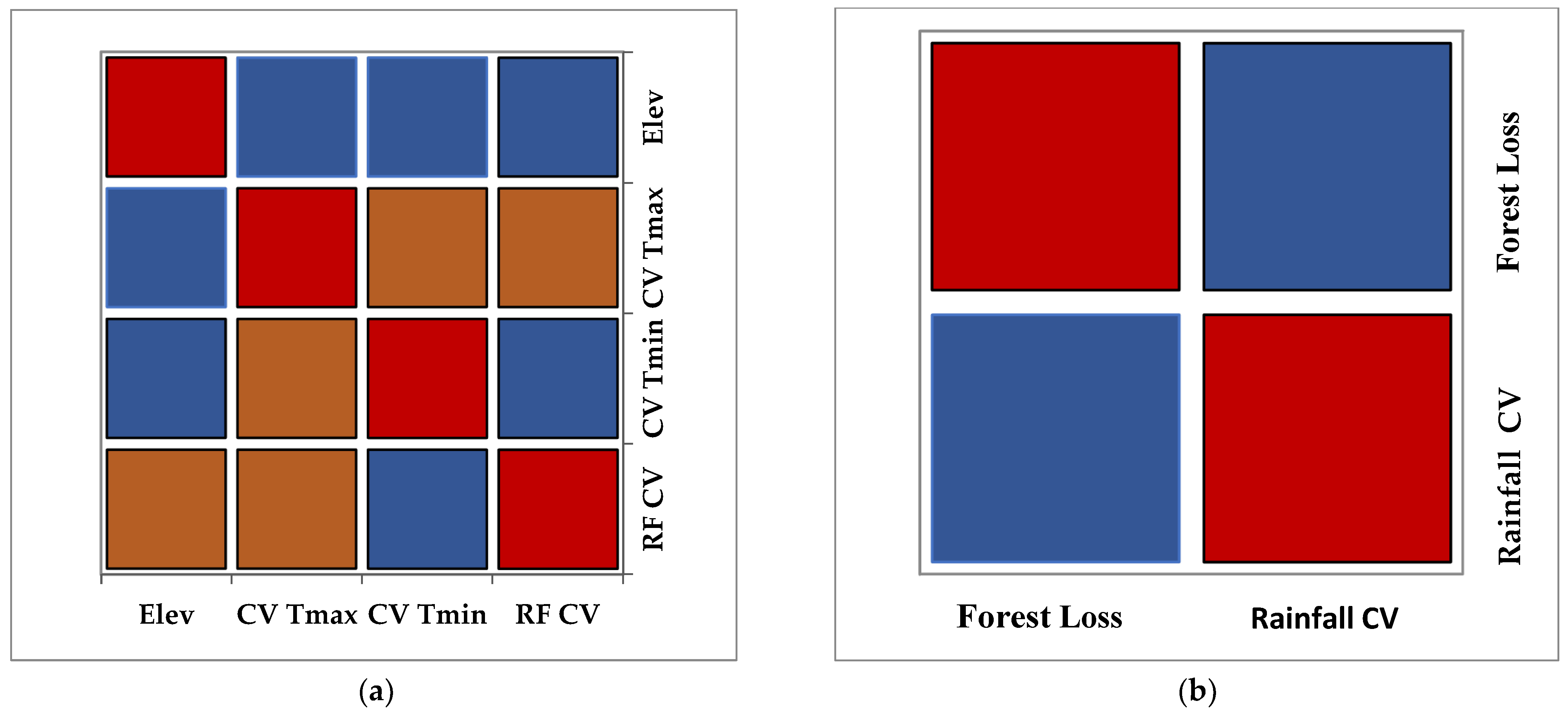
Correlation maps (a) between Elev, CV Tmax, CV Tmin, and RF CV, representing elevation, variability in maximum temperature, variability in minimum temperature, and variability in rainfall, respectively, where variability is measured by the coefficient of variation (CV); (b) between forest loss and annual rainfall variability; and (c) between catchment size (km2) and annual rainfall variability. The red color indicates a perfect match with a correlation of 1, the blue color indicates a high degree of correlation between the variables, followed by the orange color for a moderate degree of correlation, and the white color indicates a negligible relationship between the variables.
Figure 12.
Correlation maps (a) between Elev, CV Tmax, CV Tmin, and RF CV, representing elevation, variability in maximum temperature, variability in minimum temperature, and variability in rainfall, respectively, where variability is measured by the coefficient of variation (CV); (b) between forest loss and annual rainfall variability; and (c) between catchment size (km2) and annual rainfall variability. The red color indicates a perfect match with a correlation of 1, the blue color indicates a high degree of correlation between the variables, followed by the orange color for a moderate degree of correlation, and the white color indicates a negligible relationship between the variables.


Table 1.
Meteorological stations selected in this study.
| Station Name | Latitude | Longitude | Altitude | Data Period |
|---|---|---|---|---|
| Itang | 8.1667 | 34.2667 | 415 | 1980–2016 |
| Gambela | 8.25 | 34.58333 | 500 | 2000–2018 |
| Ayira | 9.1 | 35.55 | 1555 | 1987–2018 |
| Metu | 8.283333 | 35.56667 | 1711 | 1981–2018 |
| Bure | 8.2333 | 35.1 | 1750 | 1980–2018 |
| D.dolo | 8.516667 | 34.8 | 1850 | 1987–2018 |
| Alge | 8.533333 | 35.66667 | 1880 | 1987–2018 |
| Gore | 8.1333 | 35.53333 | 2033 | 1980–2018 |
| Masha | 7.75 | 35.4667 | 2282 | 1980–2018 |
| Humbi | 8.68333 | 36.01667 | 2284 | 1986–2018 |
Table 2.
The correlation analysis between precipitation and temperature with (a) elevation, (b) forest loss, and (c) catchment size, where the abbreviations are the same as defined in Figure 10 above.
Table 2.
The correlation analysis between precipitation and temperature with (a) elevation, (b) forest loss, and (c) catchment size, where the abbreviations are the same as defined in Figure 10 above.
| (a) | ||||
| Variables | Elev | CV Tmax | CV Tmin | RF CV |
| Elev | 1 | −0.533 | −0.723 | −0.471 |
| CV Tmax | −0.533 | 1 | 0.429 | 0.430 |
| CV Tmin | −0.723 | 0.429 | 1 | 0.697 |
| RF CV | −0.471 | 0.430 | 0.697 | 1 |
| (b) | ||||
| Variables | Forest loss | Annual CV | ||
| Forest loss | 1 | 0.65 | ||
| Annual RF CV | 0.65 | 1 | ||
| (c) | ||||
| Variables | Catch. size (km2) | Annual RF CV | ||
| Catch. size (km2) | 1 | −0.13 | ||
| Annual RF CV | −0.13 | 1 | ||
Publisher’s Note: MDPI stays neutral with regard to jurisdictional claims in published maps and institutional affiliations. |
© 2022 by the authors. Licensee MDPI, Basel, Switzerland. This article is an open access article distributed under the terms and conditions of the Creative Commons Attribution (CC BY) license (https://creativecommons.org/licenses/by/4.0/).
Share and Cite
MDPI and ACS Style
Kassaye, S.M.; Tadesse, T.; Tegegne, G.; Tadesse, K.E. The Sensitivity of Meteorological Dynamics to the Variability in Catchment Characteristics. Water 2022, 14, 3776. https://doi.org/10.3390/w14223776
AMA Style
Kassaye SM, Tadesse T, Tegegne G, Tadesse KE. The Sensitivity of Meteorological Dynamics to the Variability in Catchment Characteristics. Water. 2022; 14(22):3776. https://doi.org/10.3390/w14223776
Chicago/Turabian StyleKassaye, Shimelash Molla, Tsegaye Tadesse, Getachew Tegegne, and Kindie Engdaw Tadesse. 2022. "The Sensitivity of Meteorological Dynamics to the Variability in Catchment Characteristics" Water 14, no. 22: 3776. https://doi.org/10.3390/w14223776
Note that from the first issue of 2016, this journal uses article numbers instead of page numbers. See further details here.