
Linking the Community and Metacommunity Perspectives: Biotic Relationships Are Key in Benthic Diatom Ecology

1
Museo Nacional de Ciencias Naturales (CSIC), c/Serrano 115 dpdo., E-28006 Madrid, Spain
2
Instituto Cavanilles de Biodiversidad y Biología Evolutiva, University of Valencia, c/Catedrático José Beltrán 2, E-46980 Paterna, Spain
*
Author to whom correspondence should be addressed.
Water 2022, 14(23), 3805; https://doi.org/10.3390/w14233805
Submission received: 25 October 2022
/
Revised: 14 November 2022
/
Accepted: 19 November 2022
/
Published: 22 November 2022
(This article belongs to the Section Biodiversity and Functionality of Aquatic Ecosystems)
Abstract
:The ecology of benthic diatoms is scarce in diatom reviews, and it seems that the loss of interest in their local ecology (populations–communities) coincides with an increase in metacommunity studies. We include a review of the latter to highlight some unresolved issues. We aim to demonstrate the relevance of local population–community ecology for a better understanding of the metacommunity by addressing gaps such as the relevance of biotic relationships. We analyzed 132 assemblages of benthic diatoms from two neighboring catchments, with varying altitudes, lentic and lotic waters and substrates. Population–community features (e.g., populations’ relative abundance and alpha diversity) and metacommunity descriptors (e.g., beta diversity indices) were related to likely control factors such as space, catchment features, local physico-chemistry and biotic environment. Our results confirm the relevant role of local interactions between diatoms and with the biotic environment as the mechanism in assembly communities. Moreover, abiotic habitat stability enhances alternative assemblages, which are the base of the metacommunity structure, mostly by taxa sorting and mass effects. Our results suggest that in order to better disclose factors controlling metacommunities, we must study their communities at local scales where mechanisms that explain their assemblage occur, as this is the bridge to a better understanding of benthic diatom ecology.
1. Introduction
1.1. Community and Metacommunity of Benthic Diatoms: The Scale
Our purpose is to demonstrate the relevance of local population and community ecology for a better understanding of the metacommunity. Related to this, we highlight the role of biotic relationships as controlling factors which seem to be neglected in metacommunity studies. Take, for example, the case of benthic diatoms (BDs). The emergence and development of BD metacommunity analysis seems to coincide with the preclusion of more locally focused ecological studies (i.e., population and community) on BD. We advocate for a recovery of local ecology approaches, which are necessary to understand that diversity is the outcome of assembly dynamics, as recognized for plankton [1,2]. Thus, we suggest that this approach could be the bridge to a better understanding of the structure and dynamics of metacommunities (Table 1).
The main objectives in the study of BD metacommunities (Table 1) are usually to describe features such as beta diversity (hereafter βD), the underlying explanatory models [30,31] and the variance explained by their possible controlling factors (i.e., variance partitioning techniques; [32]). These BD studies are, with few exceptions, carried out over a large area and with a very different grain and lag (in the sense of [33]; Table 1). It is surprising that BD studies use the same scales as those used in studies of other (larger) aquatic organisms, such as fish [6], and that kilometric distances are considered “fine scale” for BD (e.g., [15]). This occurs even knowing that changes in scale vary the pattern arising from the same metacommunity [30,34] and reduce the possibility of cross-study comparisons [33]. In any case, it seems unquestionable that the effects of the environment as a structurer of the metacommunity are best appreciated when the scale is local and the area covered is smaller [10,12], thus avoiding geographic heterogeneity and barriers that emphasize the spatial component (e.g., [15]), and dispersal effects versus the local environment and mechanisms of interaction.
Therefore, when looking for explanations of the assemblies of BD metacommunities, we should also remember that environmental factors can control BD spatial distribution at very fine scales, for example, within a pond [35] or in a few square meters of a stream [3]. To address these questions regarding the analyzed space, we used intermediate scales compared to those mentioned in Table 1. In Bailey’s terminology [36], these would be a set of sites analyzed at a local scale (microecosystems or local communities with samples separated by less than 2 km) included in a smaller landscape mosaic of an intermediate scale (with a total area of over 3000 km2). This approach can be effective in disentangling mechanisms acting at different organizational levels of BD (populations, communities and metacommunities).
1.2. Drivers of BD Distribution: Environmental Factors, Habitat and Substrate
Environments that are stressful for different taxa (e.g., extreme values of factors, high disturbance) can act as a filter (i.e., only populations of some adapted species can grow in such conditions, and therefore beta diversity will be low). On the contrary, non-stressful environments attain a higher βD thanks to assembly processes due to the interacting species. The combination of species generates alternative communities and, therefore, a greater βD [2,37]. For years, there have been warnings that the idea of limiting factors in phytoplankton prevented a thorough interpretation of possible alternative mechanisms, such as biotic relationships (coexistence and exclusion) in the assembly process [2,38,39]. The relevance of biotic factors, such as the interaction between BD species, as a possible local control was reported decades ago [40,41], and more recently some authors have related them to community composition and spatial distribution [42,43]. However, these interactions have been neglected in BD distribution studies. The larger the area studied, the more likely it is to include environments with extreme values of abiotic factors, such as for conductivity or nutrient concentrations (Table 1), and the metacommunity will then be partly structured by this abiotic environment. In fact, the role of such factors (e.g., nutrients) can be concomitant with other factors, resulting in inconclusive patterns of response [4,23]. Including BD species abundances as potentially relevant environmental factors for other BD populations is a necessary step to elucidate if controlling factors are only abiotic or if they are also biotic. In addition, the effects of herbivores, such as fish and the allelopathic effect of macrophytes, on BD may also determine their community structure [35,44,45,46]. Therefore, biotic factors should not be overlooked in metacommunity studies as they can exert additional local control in BD predictive models at different scales [10,47]. Disentangling the role of biotic relationships as drivers of populations, communities and metacommunities is an important goal of this study. To do so, we focus on an area where local abiotic conditions are neither extreme nor disturbed.
There are other interesting pieces to this puzzle about the causes of BD species distribution that can be addressed from a local–intermediate scale approach and that we analyze in this study: the effect of substrate, habitat and altitude. Many studies have relied on analyses of BD abundances growing on easily quantifiable substrates in terms of surface area, such as rocks and cobbles (Table 1). The issue of substrate influence on organismic growth has been a long-standing topic in diatom ecology [40,48,49,50], but it is far from being solved [51]. Very few studies address the comparison of the metacommunity of stagnant water BD with that of streams (i.e., [52,53]), despite the fact that the physical features of one or the other habitat may affect community connectivity, environmental homogenization or disturbance intensity [52,54]. Altitudinal effects on diatom communities have also been a preferred topic for diatom ecologists for many years [12,15,55], but the results are, as yet, pretty inconclusive [47].
1.3. Goals of This Study
Our main goals in this paper are to disentangle the differences in environmental factors controlling populations, communities and metacommunities of BD and to test the relevance of biotic relationships and the importance of their effects at the local scale. We will delve deeper into these questions using a BD field-based study to establish the main mechanisms and processes of assembly as a “bridge” to better explain the metacommunity structure. In addition, this will provide more information about the ecology of this group of organisms that has been neglected in previous reviews which have mainly focused on planktonic diatoms [40,47,48,49,56,57].
Based on the issues mentioned here, we hypothesized that in a BD landscape of intermediate extension, which favors little variability in the intensity of disturbances (except for the obvious lotic and lentic differences): (i) α diversity will be independent of environmental factors and favored in undisturbed systems; (ii) relationships between BD populations will become very important for the assembly process, with exclusion (overdispersion) being the most relevant; (iii) βD will be higher if environmental stability favors alternative assemblages; and (iv) the metacommunity will be structured mostly by species sorting effects, particularly if we include the biotic factors as an environmental component.
The study was carried out in central Spain (Mediterranean semi-arid climate), thus widening the geographical scope of BD metacommunity knowledge, since the majority of such studies have, so far, been carried out in cold temperate environments (Table 1). We worked in two neighboring catchments with pristine ecosystems within an altitude range of 800 m.
2. Material and Methods
2.1. Field Work
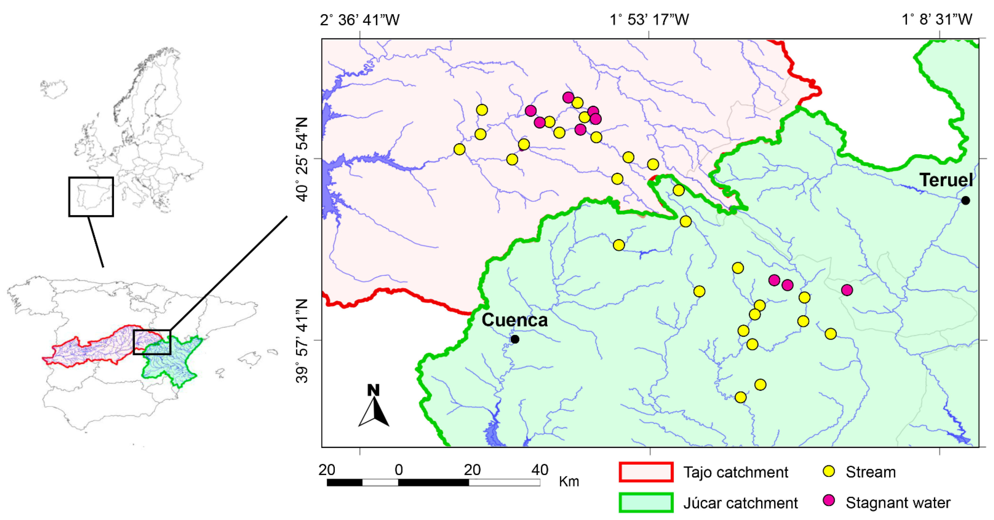
Sampling was carried out in a selected area (3588 km2) in the highest, bordering part of two large catchments (the Júcar and Tajo rivers), a mountainous region of central-eastern Spain called Serranía de Cuenca (Figure 1). The area is largely depopulated (3.5 inhabitants/km2 mostly living in small towns and villages) due to migration to eastern Spanish cities since the 1960s [4]; these trends have not changed recently, and tourism is still scarce (more information on its geography in Supplementary Materials).
The sampling locations were 36 permanent aquatic environments: 9 stagnant water bodies (i.e., lakes including springs, reservoirs and wetlands) and 27 streams (Figure 1; Table 2). Their altitude ranged from 840 masl to 1600 masl (average slopes of 4–20%). These 36 locations were visited once over a couple of weeks in summer (August 2017).
At each of these locations, samples were randomly collected on the different substrates encountered. BDs were sampled by collecting 4 colonized cobbles whose surfaces were around 20 cm2; algal materials were scraped with a brush in a composite sample and preserved in 20 mL of distilled water with 4% formaldehyde. When the substrate was different from that of the paving stones (e.g., submerged macrophyte leaves), a similar colonized surface was sought and BDs were obtained and preserved in the same way. In total, we obtained 132 samples or BD assemblages (Table S1 in Supplementary Materials). The average spacing [33] between the sites in our study was 1.7 km. This discrimination allowed us to carry out analyses both on the total number of assemblages and on sets of them in order to compare the two basins (Júcar vs. Tajo), the different habitats (stagnant water vs. streams) and the different substrates (mineral vs. vegetal). For more details, see Supplementary Materials where more specifications of the studied sites (e.g., sampling location, coordinates, type of habitat and substrate) are presented.
2.2. Data Collection Matrices
Independent variables were compiled in four matrices. Sexagesimal latitudes and longitudes were transformed into decimal data resulting in the “geographical matrix” which enabled us to calculate a matrix of Euclidean distances for further statistical analyses. The SigPac Spanish resource (sigpac.mapama.gob.es/fega/visor/, accessed on 21 October 2022) was used to derive data on the altitude, latitude, longitude, area (ha) and mean slope (%) of the sub-catchment upstream of the sampling site. Moreover, because coarser scales of spatial analyses are usually related to catchment features in stream ecology [58], the surface area of main land use types (rangeland and forests) was estimated and is either reported in absolute (ha) or relative (%) terms. Since the territory is highly depopulated (see Supplementary Materials), croplands are now kept to a minimum and they only barely surround some towns. Therefore, cropland areas were included within rangelands. These catchment features comprised the “catchment matrix”.
In situ measurements and chemical data obtained in the laboratory encompassed the raw “physico-chemical matrix”. Channel cross-section was estimated by planimetry at each sampling station, and the discharge was measured three times at a central point using a FLOW Global Water FP 101 probe. Both measurements enabled us to estimate stream water velocity. Water temperature, dissolved oxygen, pH and conductivity were measured with ODO Yellow Springs and CRISON portable equipment. Chemical analyses using [59] were undertaken shortly after water collection. Nitrogen (nitrate, nitrite and ammonia) and dissolved phosphorus compounds were measured with a Seal analyzer-3, whereas organic carbon (total, TOC hereafter, and dissolved, DOC hereafter) and total nitrogen were measured with TOC-VCSH Shimadzu equipment. Raw samples were digested with strong acids to mineralize all phosphorus forms to render total phosphorus as SRP, which was measured as above. Few data were recorded for silicon, ranging 1.05–2.08 mg Si/L, thus suggesting non-limited diatom growth [60].
The “biological matrix” was constructed with local biological variables which were likely to impinge on BD: presence of riparian arboreal vegetation, presence of herbivory (i.e., the occurrence of fish with a benthic feeding mode), plants as substrate (the details about different specific materials of substrates are provided in Table S1) and evidence of anthropogenic degradation.
BD data were used as dependent matrices. We used a qualitative presence matrix (i.e., presence/absence) to estimate BD richness and frequency of occurrence (i.e., percentage of samples where a taxon was found) and a quantitative matrix with the relative abundance of taxa in each sample. Methods for sample treatment, taxonomical classification and counts were standard and they are explained in the Supplementary Materials file.
Based on these data, statistical analyses could be carried out for the whole or for each catchment (Júcar or Tajo), for each habitat (stagnant water, stream) and for each substrate (mineral, plant).
2.3. Population–Community Structure and Its Control
To establish abiotic environmental controls, and suggest either exclusion or coexistence among diatoms, stepwise linear regression models (F-to-enter = 1) were attempted on relative abundance of main taxa and abiotic variables (catchment and physico-chemical matrices) plus biotic variables (the same relative abundance of the main taxa). We defined the main taxa for each sample set (overall, each catchment, each habitat and each substrate) as those with a relative abundance equal to, or greater than, 50% in a given sample, and that were also found in at least 40% of the samples in any of the sets. Before establishing coexistence or exclusion on the basis of a positive or negative relationship between two species, we checked that they did not have a similar relationship with environmental variables. This allowed us to rule out that the latter relationship was the main reason for their exclusion or coexistence. Stepwise linear regression was performed using the STATISTICA 7.0 software package (StatSoft Inc., Tulsa, OK, USA).
We calculated the alpha diversity (richness, Shannon index and effective number) of each local assemblage (considering all taxa). We expressed the Shannon index based on natural logarithms (nats). We transformed it into the effective number [61] which enabled us to perform ANOVAs comparing the average alpha diversity within each set of samples. We also analyzed the abiotic environmental control on alpha diversity with the same approach as above.
2.4. Metacommunity Structure, Its Control and Spatial Scales
Based on the composition of the assemblages, we calculated several measurements of βD because their information can be complementary, and it also allows us to compare with results from different authors who used different indices. Based on the presence/absence matrix, Jaccard similarity and Harrison indices of βD [62] were calculated using the PAST package [63]. Multiple-site dissimilarity measurements [31,64], i.e., the spatial turnover (species replacement between sites) and nestedness components of Jaccard dissimilarity, were estimated with the Betadiver R-program (on Jaccard’s grounds) in the vegan 2.5–6 package [65]. A nestedness metric based on overlap and decreasing fill (NODF hereafter) was also estimated [64,66]. We also measured βD by taking into account the relative abundance of the taxa [67]: the local (LCBD) and taxa (SCBD) contributions to the quantitative beta diversity. Values were calculated with the beta.div function of the adespatial R-package [68]. Bray–Curtis based ANOSIM was applied to relative abundances of taxa to detect differences in averaged similarity within a set of samples (catchments, habitats and substrates), as mediated by altitude. In order to investigate which taxa contribute the most to the variability in similarity between stagnant and stream waters, we used SIMPER analysis [69]. These analyses were performed using the PAST package [63].
To check the spatial and environmental contributions to BD metacommunity variability, partial RDA (redundancy analysis) for variance partitioning was undertaken following the procedures of [32]. The independent matrices were the spatial (geographical matrix) and environmental ones as reported below (i.e., catchment, physico-chemical and biological matrices). Correlation between environmental variables was calculated to discard collinearity inflation (>80% explained variability to each other). Variance inflation factors were estimated using the vif algorithm from the R vegan package [65]. Finally, the independent components were space and the three environmental matrices separately with their selected variables: physico-chemical (i.e., conductivity and total phosphorus), catchment features (i.e., altitude and the relative area covered by forests) and biological (i.e., substrate type, fish herbivory and riparian canopy). These new matrices were then converted into distance matrices (Euclidean distances) using the varpart program from the vegan package of R [65].
Only those taxa with a relative abundance of more than 3% in more than one sample were included in presence and relative abundance matrices [5]. After being transformed by the Hellinger approach, their Bray–Curtis similarity matrices were calculated and used as dependent matrices in RDA [32]. RDA was separately undertaken for presence and relative abundance as dependent factor.
A complementary analysis to the preceding ones is a spatial correlogram, and this was performed using the adespatial package of R [68]. Spatial autocorrelation was assessed by transforming geographical coordinates into a Euclidean distance matrix. Moran’s I and Mantel correlograms were calculated to detect autocorrelation in BD presence and relative abundance matrices. We used the Mantel correlogram function of the vegan R-package [65], and the number of computed distance classes was chosen to follow Sturge’s rule [32]. In addition, we also performed the same analysis for an environmental matrix including variables without collinearity (see above). Second-order spatial stationary conditions must, at least, be applied to meet the condition that the spatial variability in data is adequately described by the same single spatial correlation function throughout the study area [32]. This was undertaken by using the resid function of R.
3. Results
3.1. Benthic Diatom Assemblages and Their Controlling Factors
We recorded 156 benthic diatom taxa in the studied area (Table S2). The community richness ranged between 3 and 29 taxa. The average richness was higher in the Tajo catchment compared to the Júcar one, and also in stagnant water compared to streams, but no significant difference was found between epiphytic assemblages and epilithic ones (Table 3). The range of Shannon index values of all communities was 0.11–2.77 nats, and the range of effective number was 1.12–15.89. The averaged effective numbers between sets of samples did not reveal significant differences (Table 3). Therefore, diversity of taxa was not enhanced by a certain catchment, habitat or substrate. Taking into account all the assemblages, there were no relationships (p > 0.05) between α diversity metrics and abiotic environmental factors.
Eight taxa made up the most remarkable ones (i.e., dominants and/or cosmopolite; Table 3). Achnanthidium minutissimum, Cocconeis placentula and Gomphonema angustatum were the dominant taxa, with high occurrence in all sets of samples. However, other species seem more exclusive to the catchments, habitats and substrates: Cymbella affinis and Cymbopleura amphicephala mainly occurred in stagnant waters in the Tajo basin, the former mostly appearing epilithically and the latter epiphytically. Cymbella delicatula, Diatoma vulgare and Navicula cryptotenella were mainly observed in streams of the Júcar catchment and on plant substrate.
The linear models of taxa vs. environmental factors (including all BD taxa plus all variables of catchment, physico-chemical and biological matrices) showed that the variability in BD populations was usually better explained by the relationships with other BDs (i.e., exclusion, coexistence) rather than by any environmental factor (Table 4). For example, in stagnant waters, Cymbella minuta was inversely related to Cymbella affinis and Achnanthidium minutissimum, and it was positively related with Epithemia goeppertiana. These three relationships explained 80% of C. minuta relative abundance. In streams, either A. minutissimum or C. placentula happened to be inversely related with a wide array of other taxa, thus showing some exclusion evidence, albeit the explained variability was around 40% (Table 4). Negative relationships mainly occur between species of the same genus and most positive relationships between species of different genera (Table 4). Only a few populations appear to be somewhat related to the environment, and specifically Cymbella cesatii was strongly controlled by oxygen saturation (>50% of its variability; Table 4).
3.2. Metacommunity Structure: Beta Diversity
The large catchments (Júcar and Tajo) shared (Jaccard similarity index) 54% of taxa. Roughly, the same percentage of common taxa was shared between stagnant water bodies and streams. Similarity between communities from different substrate types was analyzed in detail, and the results showed that the filamentous algae substrate shared 47% of taxa with mineral substrate and 48% with macrophytes, and that mineral substrate and macrophytes shared 57% of taxa. When split altitudinally by 200 m ranges, Jaccard index values were also between 47% and 53%.
The Harrison βD was similar in both catchments, whereas that of stagnant waters and mineral substrates were greater than that of streams and epiphytic substrates, respectively (Table 3). The range of the NODF metric was 22.7–29.7, with stagnant water bodies showing the highest value (Table 3). The spatial turnover range was 0.73–0.96, and dissimilarity due to nestedness varied between 0.02 and 0.11 (Table 3). The SCBD and LCBD ranges were 0.000–00.123 and 0.005–00.013, respectively. Only the species contribution (SCBD) to βD was significant.
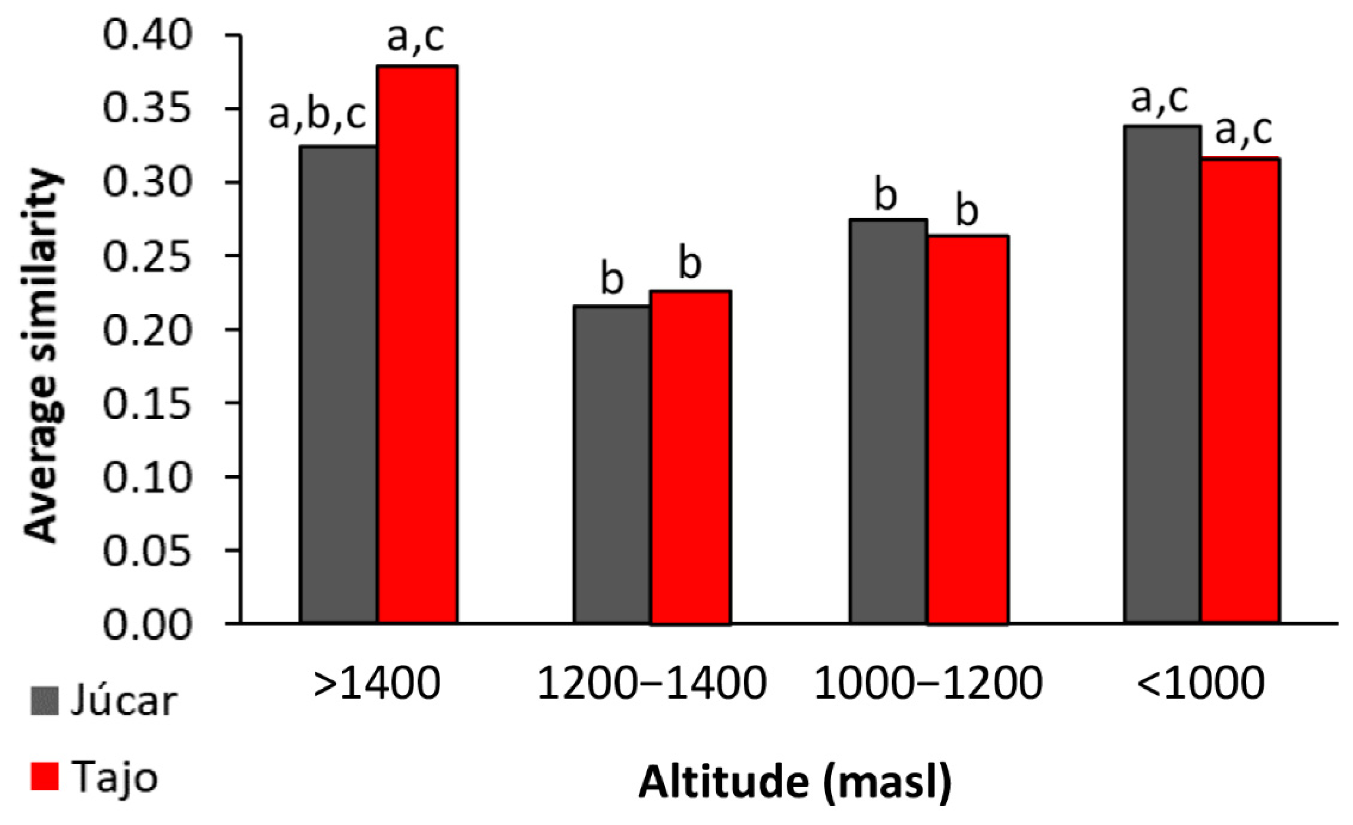
Considering the relative abundances of the taxa, the averaged similarity (ANOSIM, Bray–Curtis index) was slightly higher in the Tajo compared to the Júcar catchment (0.26 ± 0.20 vs. 0.21 ± 0.22; R2 = 0.13, p = 0.0001) and in stagnant waters compared to streams (0.28 ± 0.25 vs. 0.22 ± 0.20; R2 = 0.13, p = 0.02). Differences between substrates were not significant (p = 0.09). There was an altitudinal effect, as at intermediate altitudes (1000–1400 masl) the averaged similarities were lower than those averaged at higher and lower altitude sites (Figure 2). To detect a possible effect of the catchment on this altitudinal pattern, we compared the relative abundance of the eight distributions (two catchments x four altitudinal ranges; Figure 2) which resulted in significant differences (Kruskal–Wallis test: H-Chi2 = 107, p < 0.0001). The Mann–Whitney post hoc pairwise comparisons showed that the mean similarity at intermediate altitudes, regardless of catchment, was lower than at higher altitudes (Figure 2). Seven taxa contributed up to 60% of the dissimilarity between stagnant water and streams in each catchment (Table S3), four of which were common to both catchments: Achnanthidium minutissimum, Cocconeis placentula, Cymbopleura amphicephala and Gomphonema angustatum.
3.3. The Metacommunity: Variance Partition and Spatial Patterns
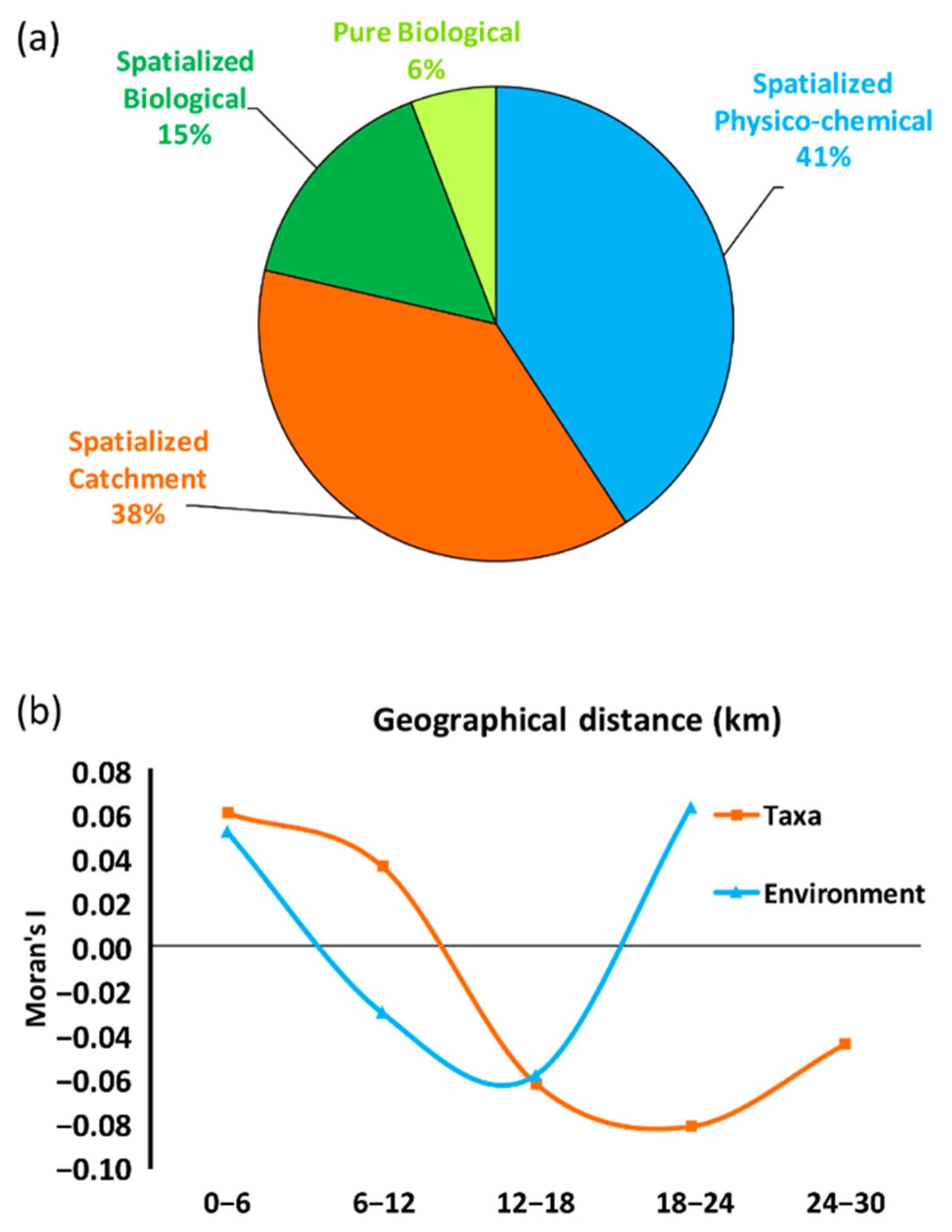
The RDA showed that both spatial and environmental factors explain both the presence and the relative abundance of taxa, and do so with similar efficiency (Table S4). We will, therefore, only detail the results on the relative abundance matrix. Unexplained variance was around 50% (Table 5 and Table S4). The pure environmental component explained at least twice the variance of relative abundance compared to the pure space component (Table 5); the rest was due to the overlap of space with environmental contributions (Figure 3a). When using the three environmental matrices (physico-chemical, catchment and biological matrices), it was the biological matrix (i.e., substrate type, fish herbivory and riparian canopy) that explained some variability independently of space (Figure 3a; Table 5), and pure space did not explain any variance. The relative abundance data, grouped by catchments, habitat or substrate (Table 5), showed less spatial intervention and slightly more variance explained in streams compared to stagnant waters and in the Júcar catchment (with a higher proportion of streams) than in the Tajo, as well as in the epilithic samples for which the highest values of variance explained by the pure biological component were observed.
The geographic variation of the BD community (Mantel’s spatial autocorrelation with Moran’s I coefficient across distance classes) was considerably different whether calculated with the species occurrence matrix or the relative species abundance matrix (Table S5). BD presence only showed autocorrelation (p = 0.028) at the shortest distance classes, and BD relative abundances followed a decreasing curve (Table S5, Figure 3b). When we estimated the autocorrelation pattern of environmental factors used above, a U-shaped pattern appeared (Table S5, Figure 3b).
4. Discussion
4.1. Benthic Diatom Populations–Communities and Their Control Factors
The paucity of BD studies has prevented the species–area relationship from being confirmed so far with a meta-analysis [47]. In fact, the disparity of these values can be seen in Table 1. For example, the richness reported here (with a study area of 3300 km2) is similar to that found in the large area of the Manyame catchment in Zimbabwe (40,000 km2; [14]) or in a smaller region in China (950 km2; [15]). To this hypothetical effect of the area, we should add the effect of the type of habitat that is mainly included in such areas. For example, [53] and ourselves, studying more than twice as many samples from streams as from stagnant water, found 25% richer communities in the latter habitats than in the former. In addition, the Júcar catchment, whose rivers:lakes ratio of samples is three times greater than that of the Tajo catchment, has the lowest richness in its communities. These results would agree with the expected lower richness in highly disturbed locations [37,70].
Furthermore, we wonder whether the type of substrate which is usually sampled should also be taken into account. So far, there is much more data on rock communities than on plants or other mineral substrates (Table 1). Perhaps subtler differences will be found when more data on substrates become available. For the time being, the richness of communities on plants and on minerals according to our results was similar, and this is also inferred from other works (e.g., [71,72,73]). In addition, we have proved that ecological diversity, measured as the effective number of species, was independent of the habitat and substrate, as other studies have also reported for the Shannon index [53,72,73]. Therefore, the fact that the selection of the sampled substrate is certainly biased towards cobbles (Table 1) does not seem to be relevant in establishing the ecological diversity of BD. At the moment, it does not seem to be different from the diversity of assemblages from, for example, plants. This is noteworthy because, otherwise, the effort to obtain the ecological diversity of assemblages from various substrates of an ecosystem would have to be extended, increasing the costs of, for example, water quality assessment. Furthermore, in the intermediate spatial extent studied here, alpha diversity does not appear to reflect changes in any environmental factors. Our first hypothesis, “α diversity will be independent of environmental factors and favored in undisturbed systems”, has been confirmed. In addition, we discovered as a corollary that the variety of habitats, and the intensity of disturbances that are amplified with the area studied, will make it difficult to find a BD species–area relationship.
Our results suggest that interactions between BD populations at the local scale should be taken into account as mechanisms involved in BD assemblage construction. These biotic relationships explain the variability in taxa distribution better than the abiotic environment. One of the main results regarding likely mechanisms implying the exclusion effect (or overdispersed distributions in the sense of [37]) was that of the opposite dominances of Achnanthidium minutissimum and Cocconeis placentula in streams, something which had already been mentioned in the 1970s [40]. More recently, [42] attributed the contrasting distribution of these two populations to a greater dispersal ability of the small A. minutissimum, a mass effect under environmentally sub-optimal conditions, versus C. placentula, which is a larger diatom and is more prone to a clumped distribution. These two dispersive strategies based on their traits allow these species to also be ubiquitous, appearing in different continents and dominant in small areas, such as the one analyzed here, or in other much larger ones ([4]; Table 1). Another mechanism would explain the contrasting distribution of Cymbella affinis and Cymbella minuta in stagnant waters (Table 3), namely, competition between very similar and fast-growing species [74], such as these ones. It has been impossible to find studies on the biology of these Cymbella species that can be related to their overdispersion distributions due to competition. Despite the fact that competition between benthic algae, as a mechanism that would explain their distribution, was suggested at the end of the 1990s [41], interactive mechanisms between BD have been scarcely addressed [43,75]. We have found positive relationships between some taxa such as Cymbella minuta and Epithemia goeppertiana (Table 3); this is possible because these two taxa have very different strategies to take advantage of the low phosphorus concentration [50,76]. In addition, the fact that most of the positive relationships occur between species of different genera, and the negative ones mainly between species of the same genus, would reinforce the idea that mechanisms avoid sharing the niche work. We consider our second hypothesis, “relationships between BD populations will become very important for the assembly process, with exclusion (overdispersion) being the most relevant“, to have been tested. Moreover, we can express another corollary: there is a small set of dominant and ubiquitous species, but they belong to different assemblages as is evident from their preferences for rivers or lakes and their overdispersion distribution in communities. This assemblage design, the coexistence of taxa recorded in the different BD communities, is reminiscent of the species associations recognized for phytoplankton which were related to the environment [77,78]. This would be an interesting avenue to pursue with BD.
4.2. Metacommunity Structure: βD Patterns
The shared BD taxa among different groups of samples was around 50%. This ubiquity of BD was independent to catchments, habitats or substrates. This component of homogeneity in communities results in a low Harrison index and weak nestedness, both indices being lower in streams than in stagnant waters. Therefore, we suggest that at the intermediate scale (two contiguous basins) studied here, it is possible to observe how the water flow homogenizes the environment that BDs inhabit. This result, along with those of [24,79], point to how homogeneous pristine rivers seem to be for diatom distribution when analyzed at these sparsely studied intermediate scales. In addition, a higher homogeneity in BD communities in streams compared to stagnant waters has been observed on other occasions (e.g., [53]), and the cause may be that higher physical connectivity in streams favors dispersion of microorganisms and environment homogenization (e.g., [9,80]).
On the other hand, a high spatial turnover and a negligible value of the nestedness component of dissimilarity means that the βD pattern in our intermediate studied region was almost exclusively caused by species replacement [64]. The spatial turnover component was greater in our study than the value recorded comparing numerous French streams at a larger scale [23]. In addition, the use of relative abundance allows us to highlight that the contribution of species to βD (SBDC) is considerably higher than the local ecological uniqueness contribution (LCBD), the latter being related to the unusual habitat conditions that select only a few taxa [81]. While the range of SCBD at the intermediate spatial scale used here was greater than that of other studies of diatoms over a large regional scale, our range of LCBD was within their reported ranges [19,26,29]. The SCBD reflects the fact, already described here, that there is a small group of dominant species (only seven species are responsible for the dissimilarity) which are also the most ubiquitous and are exclusive of each other (e.g., A. minutissimum and C. placentula), and all other species are rare. This seems to be the BD metacommunity pattern, both at intermediate and large spatial scales such as the one studied by [19]. Therefore, the mechanisms underlying this pattern, supported by the above analysis of population controlling factors and compositions of communities, seems to be biotic interactions between BDs in the assembly process instead of a selective environment factor acting as a filter for main populations. The assembly process as a mechanism of main species sorting is reflected in the high turnover and rare species following a mass effect or a stochastic distribution. As the replacement pattern predominates between BD communities, the maintenance of their biodiversity involves the conservation of communities of different localities with a criterion of floristic complementarity [26,31].
When looking at βD at different altitudes, we found other possible evidence that higher environmental stability implies greater beta diversity as a result of the assembly process: the highest βD occurs among the communities at intermediate altitudes. Despite the reduced altitudinal range (840–1600 masl) studied here, the climatic gradient could be considered a driver of altitudinal variation in βD [47] because temperature was one of the few local environmental factors explaining variance in some BD populations. At headwaters, or higher altitude, climate acts as a filter, while downstream, or at lower altitudes, high pollution or anthropic degradation would be another filter (nitrogen being the other somewhat significant factor for populations).
Therefore, we consider our third hypothesis (i.e., βD will be higher if environmental stability favors alternative assemblages), linking stability to the possibility that assemblage processes lead to different communities by combining a set of species, to be proven. Even in a small–intermediate area with little altitudinal variation, we detected lower βD in lotic habitats compared to lentic habitats and at more disturbed altitudes. Further studies on BD are needed to understand the relationship between all the different βD metrics and their underlying explanatory mechanisms and processes [9,43,82,83,84]. For the time being, to unravel the βD components [67] of BD metacommunities the use of pre-existing databases could be of interest (Table 1).
4.3. The Metacommunity: Variance Partition and Spatial Patterns
Presence and relative abundance were explained by both space and environment, as reported by other studies (Table 1). Relatively high unexplained variability often occurs in many metacommunity studies as a result of overlooked factors, stochasticity, interactions with unconsidered taxa, etc. [26,85]. Presence and relative abundance both showed similar good results (Table S4) and are therefore recommended for the monitoring of BD metacommunities [26,47]. Pure environment, without space overlap, explained double the variance compared to pure space (Table 5; Figure 3a). The importance of environmental factors for diatom metacommunities has already been emphasized by [10]. Ref. [12] suggested that it is in small areas, such as those used in this study, where more variability purely explained by the environment is experienced, because geographical features in larger extents may mask it. Related to this, pure space did not explain the variance, or explained very little variance in the Serranía of Cuenca area. In a slightly larger area, pure space was found to be significant ([5]; Table 1), but the author suggested that this spatial variance was due to a spatial gradient of land use attributes. In our study, landscape or catchment variables, such as land use, were already included in environmental matrices, and therefore our result concerning structuring due strictly to space clearly shows the dispersive capabilities of BD populations. To our knowledge (Table 1), this is the smallest extent to which pure space explained some, albeit little, variance in BD. We verified that it is in streams where metacommunity structure was better explained, especially by the environment, as was also observed by [10]. When treating space together with physico-chemical, catchment and biological matrices separately, the biological variables (i.e., riparian canopy, substrate types and fish herbivory) were the ones that purely explained the variance. This fact highlights that biological relationships at the local scale are important in the structuring of the metacommunity [10]. All these results encourage the inclusion of more biotic variables, such as the presence of bacteria, other benthic algae or macroinvertebrates strongly linked to BD growth [43,86] or the three-dimensional mode of their community [87]. We should test whether the addition of new local biotic variables, relevant to the growth of BD, help us to understand the drivers in the structuring of their metacommunity.
The weak effect of space versus environment suggests that the BD metacommunities studied here arise largely from species sorting, and from species sorting plus mass effect processes [30,34,85], as inferred from the above βD analysis and as expected in small areas [47], confirming our fourth hypothesis. In conclusion, we found that local interspecific relationships, or the process of community assembly, were the mechanisms explaining βD (i.e., we highlight the relevance of interspecific biotic relationships) and that BD relationships with local biological conditions shape the metacommunity structure and explain its construction pattern.
In addition, the above conclusions on the relevance of local factors structuring communities and the metacommunity was reinforced when disentangling the patch structure over different spatial scales. An initial positive value of autocorrelation at the smallest scale (less than six kilometers) was followed by significant negative values at larger scales, tens of kilometers, as detected by [6] in a fragmented French river. The correlogram of the environment also showed similar positive values at the finest spatial scale, confirming that the environment structures the spatial patterns of the BD at this scale (zone of influence, sensu [88]).
Finally, we would like to draw attention to the fact that both the metacommunity archetypes (species sorting, species sorting plus mass effect) and the scale of interaction with the environment have been described not only for small but also for large extents and coarser scales [4,16] addressing similar goals about the spatial ecology of BD (Table 1). This may be a serious inconsistency that has long been detected in both geography and ecology [89,90] and may prevent cross-comparison of studies [33]. In short, we need to understand the environmental factors acting at the microscopic scale as determinants of organismal ecology (e.g., inside the biofilm; [43]), the local factors of the environment where BD assembly occurs and the community develops [57] and at a broader scale the environmental patterns defining macroecological rules [91]. Based on the confirmation of our fourth hypothesis, we encourage the analysis of the local communities’ drivers to understand the metacommunity structure.
5. Conclusions
As in an experimental design in which almost all conditions are set to analyze the variability in a variable in depth, we wanted to show, with the use of an intermediate spatial extent and the inclusion of many biotic variables, that biotic relationships occur that explain the presence of populations and the organisation of communities that ultimately structure the metacommunity. As a result of the implementation of conservation directives and concerns about global change, there are a large number of quantitative BD datasets available worldwide that could be a very good basis for (following our recommendation) achieving a better understanding of BD ecology. Some conclusions of our work, due to their relevance in applied ecology, should be tested in more environments, e.g., the indifference of assembled BD to different substrates and the poor response of diversity indices to environmental changes. Finally, we call for future work on the analysis of the relationships that structure communities (populations with their biotic and abiotic environment) at local scales as a basis for understanding the mechanisms underlying environmentally explained variance in metacommunity structure.
Supplementary Materials
The following supporting information can be downloaded at: https://www.mdpi.com/article/10.3390/w14233805/s1, Figure S1: Clusters of contiguous sites calculated on the taxa matrix; Table S1: 132 samples. Description of the substrate in the samples; Table S2: Taxa and taxa codes; Table S3: Benthic diatoms taxa which contribute more to dissimilarities between samples. SIMPER results; Table S4: RDA results about variance explained by space and environment. Dependent variables were presence and relative abundance of benthic diatoms taxa (BD); Table S5: Spatial autocorrelograms (Moran’s I) of taxa and environment. References [92,93,94,95,96,97,98,99,100,101,102] are cited in the Supplementary Materials.
Author Contributions
Conceptualization: C.R. and M.Á.-C.; Methodology: C.R. and M.Á.-C.; Formal analysis: C.R. and M.Á.-C.; Investigation resources: C.R. and M.Á.-C.; Writing-original draft preparation: C.R. and M.Á.-C.; Writing-Review and editing: C.R. All authors have read and agreed to the published version of the manuscript.
Funding
This research received no external funding.
Institutional Review Board Statement
Not applicable.
Informed Consent Statement
Not applicable.
Data Availability Statement
Data are available from the RODERIC Digital Repository: https://hdl.handle.net/10550/75666. Accessed on 21 October 2022.
Acknowledgments
Matilde Segura advised us on taxonomic determinations, Eric Puche and Daniel Sheerin helped us to obtain a better editing of the manuscript. This study is dedicated to the seminal scholars of diatom ecology: Robert Wilhelm Kolbe, Bela Jeno Cholnoky and Ruth Marie Patrick.
Conflicts of Interest
The authors declare no conflict of interest.
References
- Rojo, C.; Rodrigo, M.A.; Álvarez-Cobelas, M. Plankton diversity as an outcome of the assembly process. SIL Proc. 1922–2010 2006, 29, 1906–1908. [Google Scholar] [CrossRef]
- Rojo, C. Community assembly: Perspectives from phytoplankton’s studies. Hydrobiologia 2021, 848, 31–52. [Google Scholar] [CrossRef]
- Passy, S.I. Spatial paradigms of lotic diatom distribution: A landscape ecology perspective. J. Phycol. 2001, 37, 370–378. [Google Scholar] [CrossRef]
- Potapova, M.G.; Charles, D.F. Benthic diatoms in USA rivers: Distributions along spatial and environmental gradients. J. Biogeogr. 2002, 29, 167–187. [Google Scholar] [CrossRef]
- Passy, S. Community analysis in stream biomonitoring: What we measure and what we don’t. Environ. Monit. Assess. 2007, 127, 409–417. [Google Scholar] [CrossRef]
- Grenouillet, G.; Brosse, S.; Tudesque, L.; Lek, S.; Baraillé, Y.; Loot, G. Concordance among stream communities and spatial autocorrelation along a fragmented gradient. Divers. Distrib. 2008, 14, 592–603. [Google Scholar] [CrossRef]
- Soininen, J. The ecological characteristics of idiosyncratic and nested diatoms. Protist 2008, 159, 65–72. [Google Scholar] [CrossRef]
- Urrea, G.; Sabater, S. Epilithic diatom assemblages and their relationship to environmental characteristics in an agricultural watershed (Guadiana River, SW Spain). Ecol. Indic. 2009, 9, 693–703. [Google Scholar] [CrossRef]
- Soininen, J.; Kongas, P. Analysis of nestedness in freshwater communities—Patterns across taxa and trophic levels. Freshw. Sci. 2012, 31, 1145–1155. [Google Scholar] [CrossRef]
- Göthe, E.; Angeler, D.G.; Gottschalk, S.; Löfgren, S.; Sandin, L. The influence of environmental, biotic and spatial factors on diatom metacommunity structure in Swedish headwater streams. PLoS ONE 2013, 8, e72237. [Google Scholar] [CrossRef]
- Tornés, E.; Ruhí, A. Flow intermittency decreases nestedness and specialization of diatom communities in Mediterranean rivers. Freshw. Biol. 2013, 58, 2555–2566. [Google Scholar] [CrossRef]
- Bottin, M.; Soininen, J.; Ferrol, M.; Tison-Rosebery, J. Do spatial patterns of benthic diatom communities vary across regions and years? Freshw. Sci. 2014, 33, 402–416. [Google Scholar] [CrossRef]
- Winegardner, A.; Beisner, B.; Legendre, P.; Gregory-Eaves, I. Are the landscape-level drivers of water column and surface sediment diatoms different? Freshw. Biol. 2015, 60, 267–281. [Google Scholar] [CrossRef]
- Bere, T.; Mangadze, T.; Mwedzi, T. Variation partitioning of diatom taxa data matrices: Understanding the influence of multiple factors on benthic diatom communities in tropical streams. Sci. Total Environ. 2016, 566-567, 1604–1613. [Google Scholar] [CrossRef]
- Dong, X.; Li, B.; He, F.; Gu, Y.; Sun, M.; Zhang, H.; Tan, L.; Xiao, W.; Liu, S.; Cai, Q. Flow directionality, mountain barriers and functional traits determine diatom metacommunity structuring of high mountain streams. Sci. Rep. 2016, 6, 24711. [Google Scholar] [CrossRef] [Green Version]
- Soininen, J.; Jamoneau, A.; Rosebery, J.; Passy, S.I. Global patterns and drivers of taxa and trait composition in diatoms. Global Ecol. Biogeogr. 2016, 25, 940–950. [Google Scholar] [CrossRef]
- Virtanen, L.K.; Soininen, J. Temporal variation in community–environment relationships and stream classifications in benthic diatoms: Implications for bioassessment. Limnologica 2016, 58, 11–19. [Google Scholar] [CrossRef]
- Heino, J.; Soininen, J.; Alahuhta, J.; Lappalainen, J.; Virtanen, R. Metacommunity ecology meets biogeography: Effects of geographical region, spatial dynamics and environmental filtering on community structure in aquatic organisms. Oecologia 2017, 183, 121–137. [Google Scholar] [CrossRef] [Green Version]
- Vilmi, A.; Karjalainen, S.M.; Heino, J. Ecological uniqueness of stream and lake diatom communities shows different macroecological patterns. Divers. Distrib. 2017, 23, 1042–1053. [Google Scholar] [CrossRef] [Green Version]
- Teittinen, A.; Wang, J.; Strömgård, S.; Soininen, J. Local and geographical factors jointly drive elevational patterns in three microbial groups across subarctic ponds. Global Ecol. Biogeogr. 2017, 26, 973–982. [Google Scholar] [CrossRef]
- Virta, L.; Soininen, J. Distribution patterns of epilithic diatoms along climatic, spatial and physicochemical variables in the Baltic Sea. Helgoland Mar. Res. 2017, 71, 16. [Google Scholar] [CrossRef]
- Winegardner, A.; Legendre, P.; Beisner, B.E.; Gregory-Eaves, I. Diatom diversity patterns over the past c. 150 years across the conterminous United States of America: Identifying mechanisms behind beta diversity. Global Ecol. Biogeogr. 2017, 26, 1303–1315. [Google Scholar] [CrossRef]
- Jamoneau, A.; Passy, S.I.; Soininen, J.; Leboucher, T.; Tison-Rosebery, J. Beta diversity of diatom taxa and ecological guilds: Response to environmental and spatial mechanisms along the stream watercourse. Freshw. Biol. 2018, 63, 62–73. [Google Scholar] [CrossRef] [Green Version]
- Jyrkänkallio-Mikkola, J.; Heino, J.; Soininen, J. Beta diversity of stream diatoms at two hierarchical spatial scales: Implications for biomonitoring. Freshw. Biol. 2016, 61, 239–250. [Google Scholar] [CrossRef]
- Passy, S.I.; Larson, C.A.; Jamoneau, A.; Budnick, W. Biogeographical patterns of species richness and abundance distribution in stream diatoms are driven by climate and water chemistry. Am. Nat. 2018, 192, 605–617. [Google Scholar] [CrossRef] [Green Version]
- Szabó, B.; Lengyel, E.; Padisák, J.; Stenger-Kovács, C. Benthic diatom metacommunity across small freshwater lakes: Driving mechanisms, β-diversity and ecological uniqueness. Hydrobiologia 2019, 828, 183–198. [Google Scholar] [CrossRef]
- Rodríguez-Alcalá, O.; Blanco, S.; García-Girón, J.; Jeppesen, E.; Irvine, K.; Nõges, P.; Nõges, T.; Gross, E.M.; Bécares, E. Beta diversity of stream diatoms at two hierarchical spatial scales: Implications for biomonitoring. Sci. Total Environ. 2020, 61, 239–250. [Google Scholar] [CrossRef]
- González-Trujillo, J.D.; Pedraza-Garzón, E.; Donato-Rondon, J.C.; Sabater, S. Ecoregional Characteristics Drive the Distribution Patterns of Neotropical Stream Diatoms. J. Phycol. 2020, 56, 1053–1065. [Google Scholar] [CrossRef]
- Stoof-Leichsenring, K.R.; Dulias, K.; Biskaborn, B.K.; Pestryakova, L.A.; Herzschuh, U. Lake-depth related pattern of genetic and morphological diatom diversity in boreal Lake Bolshoe Toko, Eastern Siberia. PLoS ONE 2020, 15, e0230284. [Google Scholar] [CrossRef] [Green Version]
- Leibold, M.A.; Holyoak, M.; Mouquet, N.; Amarasekare, P.; Chase, J.M.; Hoopes, M.F.; Holt, R.D.; Shurin, J.B.; Law, R.; Tilman, D.; et al. The metacommunity concept: A framework for multi-scale community ecology. Ecol. Lett. 2004, 7, 601–613. [Google Scholar] [CrossRef]
- Baselga, A. The relationship between species replacement, dissimilarity derived from nestedness, and nestednes. Global Ecol. Biogeogr. 2012, 21, 1223–1232. [Google Scholar] [CrossRef]
- Borcard, D.; Gillet, F.; Legendre, P. Numerical Ecology with R, 2nd ed.; Springer International Publishing: Cham, Switzerland, 2018. [Google Scholar] [CrossRef]
- Dungan, J.L.; Perry, J.N.; Dale, M.R.T.; Legendre, P.; Citron-Pousty, S.; Fortin, M.-J.; Jakomulska, A.; Miriti, M.; Rosenberg, M.S. A balanced view of scale in spatial statistical analysis. Ecography 2002, 25, 626–640. [Google Scholar] [CrossRef] [Green Version]
- Cottenie, K. Integrating environmental and spatial processes in ecological community dynamics. Ecol. Lett. 2005, 8, 1175–1182. [Google Scholar] [CrossRef]
- Rojo, C.; Mosquera, Z.; Álvarez-Cobelas, M.; Segura, M. Microalgal and cyanobacterial communities on charophytes: A metacommunity perspective. Fund. Appl. Limnol. 2017, 190, 97–115. [Google Scholar] [CrossRef]
- Bailey, R.G. Ecosystem Geography: From Ecoregions to Sites; Springer Science & Business: New York, NY, USA, 2009. [Google Scholar]
- Weiher, E.; Keddy, P. Ecological Assembly Rules: Perspectives, Advances, Retreats; Cambridge University Press: Cambridge, UK, 1999. [Google Scholar]
- Chorus, I.; Spijkerman, E. What Colin Reynolds could tell us about nutrient limitation, N:P ratios and eutrophication control. Hydrobiologia 2021, 848, 95–111. [Google Scholar] [CrossRef]
- Naselli-Flores, L.; Dokulil, M.T.; Elliott, J.A.; Padisák, J. New, old and evergreen frontiers in freshwater phytoplankton ecology: The legacy of Colin, S. Reynolds. Hydrobiologia 2021, 848, 1–6. [Google Scholar] [CrossRef]
- Patrick, R.M. Ecology of freshwater diatoms and diatom communities. In The Biology of Diatoms; Werner, D., Ed.; Blackwell Scientific Publications: Oxford, UK, 1977; pp. 284–332. [Google Scholar]
- McCormick, P.V. Resource competition and taxa coexistence in freshwater benthic communities. In Algal Ecology—Freshwater Benthic Ecosystems; Stevenson, R.J., Bothwell, M.L., Lowe, R.L., Eds.; Academic Press: London, UK, 1996; pp. 229–252. [Google Scholar]
- Tang, T.; Wu, N.; Li, F.; Fu, X.; Cai, Q. Disentangling the roles of spatial and environmental variables in shaping benthic algal communities in rivers of central and northern China. Aquat Ecol. 2013, 47, 453–466. [Google Scholar] [CrossRef]
- Romaní, A.M.; Guasch, H.; Balaguer, M.D. Aquatic Biofilms: Ecology, Water Quality and Wastewater Treatment; Caister Academic Press: Norfolk, UK, 2016. [Google Scholar] [CrossRef] [Green Version]
- Tall, L.; Cloutier, L.; Cattaneo, A. Grazer-diatom size relationships in an epiphytic community. Limnol. Oceanogr. 2006, 51, 1211–1216. [Google Scholar] [CrossRef]
- Passy, S.I. Diatom ecological guilds display distinct and predictable behavior along nutrient and disturbance gradients in running waters. Aquat. Bot. 2007, 86, 171–178. [Google Scholar] [CrossRef]
- Rojo, C.; Segura, M.; Rodrigo, M.A. The allelopathic capacity of submerged macrophytes shapes the microalgal communities from a recently restored coastal wetland. Ecol. Eng. 2013, 58, 149–155. [Google Scholar] [CrossRef]
- Soininen, J.; Teittinen, A. Fifteen important questions in the spatial ecology of diatoms. Freshw. Biol. 2019, 64, 2071–2083. [Google Scholar] [CrossRef] [Green Version]
- Kolbe, R.W. Grundlinien einer allgemeinen Ökologie der Diatomeen. In Ergebnisse der Biologie, 8; Von Fritsch, K., Goldschmidt, R., Ruhland, W., Eds.; Verlag von Julius Springer: Berlin, Germany, 1932; pp. 221–348. [Google Scholar]
- Cholnoky, B.J. Okologie der Diatomeen in Binnengewässern; J. Cramer: Lehre, Germany, 1968; p. 699. [Google Scholar]
- Burkholder, J.M. Interactions of benthic algae with their substrata. In Algal Ecology—Freshwater Benthic Ecosystems; Stevenson, R.J., Bothwell, M.L., Lowe, R.L., Eds.; Academic Press: London, UK, 1996; pp. 253–297. [Google Scholar]
- Letáková, M.; Fránková, M.; Poulíčková, A. Ecology and applications of freshwater epiphytic diatoms—Review. Cryptogamie Algol. 2018, 39, 3–22. [Google Scholar] [CrossRef]
- Soininen, J.; Weckström, J. Diatom community structure along environmental and spatial gradients in lakes and streams. Fund. Appl. Limnol. 2009, 174, 205–213. [Google Scholar] [CrossRef]
- Kahlert, M.; Gottschalk, S. Differences in benthic diatom communities between streams and lakes in Sweden and implications for ecological assessment. Freshw. Sci. 2014, 33, 655–669. [Google Scholar] [CrossRef]
- Liu, J.; Soininen, J.; Han, B.-P.; Declerck, S.A.J. Effects of connectivity, dispersal directionality and functional traits on the metacommunity structure of river benthic diatoms. J. Biogeogr. 2013, 40, 2238–2248. [Google Scholar] [CrossRef]
- Mereschkowsky, C. Diatomées du Tibet; Imperial Russkoe Geograficheskoe Obshchestvo: St. Petersburg, Russia, 1906. [Google Scholar]
- Cantonati, M.; Lowe, R.L. Lake benthic algae: Toward an understanding of their ecology. Freshw. Sci. 2014, 33, 475–486. [Google Scholar] [CrossRef]
- Poulíčková, A.; Manoylov, K. Ecology of freshwater diatoms—Current trends and applications. In Diatoms: Fundamentals and Applications; Seckbach, J., Gordon, R., Eds.; Scrivener Publishing LLC: Beverly, MA, USA, 2019; pp. 289–309. [Google Scholar]
- Johnson, L.; Richards, C.; Host, G.; Arthur, J. Landscape influences on water chemistry in Midwestern stream ecosystems. Freshw. Biol. 1997, 37, 193–208. [Google Scholar] [CrossRef]
- APHA. Standard Methods for the Examination of Water and Wastewater, 21st ed.; American Public Health Association/American Water Works Association/Water Environment Federation: Wasington, DC, USA, 2005. [Google Scholar]
- Carrick, H.J.; Lowe, R.L. Nutrient limitation of benthic algae in Lake Michigan: The role of silica. J. Phycol. 2007, 43, 228–234. [Google Scholar] [CrossRef]
- Jost, L.; DeVries, P.; Walla, T.; Greeney, H.; Chao, A.; Ricotta, C. Partitioning diversity for conservation analyses. Divers. Distrib. 2010, 16, 65–76. [Google Scholar] [CrossRef]
- Koleff, P.; Gaston, K.J.; Lennon, J.J. Measuring beta diversity for presence-absence data. J. Ecol. 2003, 72, 367–382. [Google Scholar] [CrossRef] [Green Version]
- Hammer, Ø.; Harper, D.A.T.; Ryan, P.D. PAST: Paleontological Statistics Software Package for education and data analysis. Palaeontol. Electron. 2001, 4, 1–9. [Google Scholar]
- Baselga, A. Partitioning the turnover and nestedness components of beta diversity. Global Ecol. Biogeogr. 2010, 19, 134–143. [Google Scholar] [CrossRef]
- Oksanen, J.; Blanchet, F.G.; Friendly, M.; Kindt, R.; Legendre, P.; McGlinn, D.; Minchin, P.R.; O’Hara, R.B.; Simpson, G.L.; Solymos, P.; et al. Vegan: Community Ecology Package; R Package Version 2.5-6. 2019. Available online: https://cran.r-project.org/web/packages/vegan/index.html (accessed on 21 October 2022).
- Almeida-Neto, M.; Guimarães, P.; Guimarães, P.R.; Loyola, R.D.; Ulrich, W. A consistent metric for nestedness analysis in ecological systems: Reconciling concept and measurement. Oikos 2008, 117, 1227–1239. [Google Scholar] [CrossRef]
- Legendre, P.; De Cáceres, M. Beta diversity as the variance of community data: Dissimilarity coefficients and partitioning. Ecol. Lett. 2013, 16, 951–963. [Google Scholar] [CrossRef]
- Dray, S.; Bauman, D.; Blanchet, G.; Borcard, D.; Clappe, S.; Guenard, G.; Jombart, T.; Larocque, G.; Legendre, P.; Madi, N.; et al. Adespatial: Multivariate Multiscale Spatial Analysis; R Package Version 0.3-8. 2020. Available online: https://github.com/sdray/adespatial (accessed on 21 October 2022).
- Clarke, K.R. Non-parametric multivariate analysis of changes in community structure. Aust. J. Ecol. 1993, 18, 117–143. [Google Scholar] [CrossRef]
- Connell, J.H. Diversity in Tropical Rain Forests and Coral Reefs: High diversity of trees and corals is maintained only in a nonequilibrium state. Science 1978, 199, 1302–1310. [Google Scholar] [CrossRef] [Green Version]
- Ivanov, P.; Kirilova, E. Benthic diatom assemblages from different substrates of the Iskar River, Bulgaria. In Eighteenth International Diatom Symposium 2004; Witkowski, A., Ed.; Biopress Limited: Bristol, UK, 2006; pp. 107–124. [Google Scholar]
- Mendes, T.; Almeida, S.F.P.; Feio, M.J. Assessment of rivers using diatoms: Effect of substrate and evaluation method. Fund. Appl. Limnol. 2012, 179, 267–279. [Google Scholar] [CrossRef]
- Wojtal, A.; Sobczyk, L. The influence of substrates and physicochemical factors on the composition of diatom communities in karst springs and their applicability in water-quality assessment. Hydrobiologia 2012, 695, 97–108. [Google Scholar] [CrossRef] [Green Version]
- Lürling, M. Grazing resistance in phytoplankton. Hydrobiologia 2021, 848, 237–249. [Google Scholar] [CrossRef]
- Heino, J.; Soininen, J. Assembly rules and community models for unicellular organisms: Patterns in diatoms of boreal streams. Freshw. Biol. 2005, 50, 567–577. [Google Scholar] [CrossRef]
- Cantonati, M.; Scola, S.; Angeli, N.; Guella, G.; Frassanito, R. Environmental controls of epilithic diatom depth distribution in an oligotrophic lake characterised by marked water-level fluctuations. Eur. J. Phycol. 2009, 44, 15–29. [Google Scholar] [CrossRef]
- Padisák, J.; Reynolds, C.S. Selection of phytoplankton associations in Lake Balaton, Hungary, in response to eutrophication and restoration measures, with special reference to the cyanoprokaryotes. Hydrobiologia 1998, 384, 41–53. [Google Scholar] [CrossRef]
- Reynolds, C.S.; Dokulil, M.T.; Padisák, J. The Trophic Spectrum Revisited—Developments in Hydrobiology 150; Springer: Dordrecht, The Netherlands, 2000. [Google Scholar]
- Hollingsworth, E.K.; Vis, M.L. The spatial heterogeneity of diatoms in eight southeastern Ohio streams: How far does a single riffle reach? Hydrobiologia 2010, 651, 173–184. [Google Scholar] [CrossRef]
- Heino, J.; Melo, A.S.; Siqueira, T.; Soininen, J.; Valanko, S.; Bini, L.M. Metacommunity organisation, spatial extent and dispersal in aquatic systems: Patterns, processes and prospects. Freshw. Biol. 2015, 60, 845–869. [Google Scholar] [CrossRef]
- Heino, J.; Grönroos, M. Exploring species and site contributions to beta diversity in stream insect communities. Oecologia 2017, 183, 151–160. [Google Scholar] [CrossRef] [Green Version]
- Leibold, M.A.; Mikkelson, G.M. Coherence, species turnover, and boundary clumping: Elements of metacommunity structure. Oikos 2002, 97, 237–250. [Google Scholar] [CrossRef] [Green Version]
- Ulrich, W.; Almeida-Neto, M.; Gotelli, N.J. A consumer’s guide to nestedness analysis. Oikos 2009, 118, 3–17. [Google Scholar] [CrossRef]
- Podani, J.; Schmera, D. A new conceptual and methodological framework for exploring and explaining patterns in presence-absence data. Oikos 2011, 120, 1625–1638. [Google Scholar] [CrossRef]
- Leibold, M.A.; Chase, J.M. Metacommunity Ecology; Princeton University Press: Princeton, NJ, USA, 2018. [Google Scholar]
- Hagerthey, S.E.; Defew, E.C.; Paterson, D.M. Influence of Corophium volutator and Hydrobia ulvae on intertidal benthic diatom assemblages under different nutrient and temperature regimes. Mar. Ecol. Prog. Ser. 2002, 245, 47–59. [Google Scholar] [CrossRef]
- Murdock, J.N.; Dodds, W.K. Linking benthic algal biomass to stream substratum topography. J. Phycol. 2007, 43, 449–460. [Google Scholar] [CrossRef]
- Legendre, P.; Fortin, M.J. Spatial pattern and ecological analysis. Vegetatio 1989, 80, 107–138. [Google Scholar] [CrossRef]
- Gehlke, C.E.; Biehl, K. Certain effects of grouping upon the size of the correlation coefficient in census tract material. J. Am. Stat. Assoc. 1934, 29, 169–170. [Google Scholar] [CrossRef]
- Jelinski, J.G.; Wu, D.E. The modifiable areal unit problem and implications for landscape ecology. Landscape Ecol. 1996, 11, 129–140. [Google Scholar] [CrossRef]
- Dickey, J.R.; Swenie, R.A.; Turner, S.C.; Winfrey, C.C.; Yaffar, D.; Padukone, A.; Beals, K.K.; Sheldon, K.S.; Kivlin, S.N. The Utility of Macroecological Rules for Microbial Biogeography. Front. Ecol. Evol. 2021, 9, 633155. [Google Scholar] [CrossRef]
- Aemet. Atlas Climático Ibérico. Temperatura del aire y Precipitación (1971–2000); Agencia Estatal de Meteorología: Madrid, Spain, 2011. [Google Scholar]
- Soil Survey Staff. Soil Taxonomy: A basic System of Soil Classification for making and interpreting Soil Surveys, 2nd ed.; Handbook 436; Natural Resources Conservation Service. U.S. Department of Agriculture: Washington, DC, USA, 1999.
- Guerra, M.A. Fuentes y manantiales de la Serranía conquense; Diputación de Cuenca: Cuenca, Spain, 1999; 241p. [Google Scholar]
- Cava, L.E. La Serranía alta de Cuenca. Evolución de los usos del suelo y problemática socioterritorial; Universidad Internacional Menéndez Pelayo y Programa LEADER Serranía de Cuenca: Cuenca, Spain, 1994; 588p. [Google Scholar]
- Álvarez-Cobelas, M.; Rojo, C.; Sánchez-Carrillo, S. Nutrient export from largely pristine catchments (Serranía de Cuenca, Central Spain). Bol. Geol. Min. 2020, 131, 559–580. [Google Scholar] [CrossRef]
- Mayoral, O. Estudio Florístico y Aportaciones a la Conservación del alto Cabriel (Cuenca). Doctoral Thesis, University of Valencia, Valencia, Spain, 2011; 554p. [Google Scholar]
- Buil, J.R.; Fernández Yuste, A.; Lozano, J.; Nicolás, I. Datos sobre la distribución de peces en los ríos de la provincia de Cuenca. Ecología 1987, 1, 231–245. [Google Scholar]
- González Guerrero, P. Novedades biológicas en algas de Cuenca. Anales Jard. Bot. Madrid 1940, 1, 107–139. [Google Scholar]
- Blanco, S.; Álvarez, I.; Cejudo, C. A test on different aspects of diatom processing techniques. J. Appl. Phycol. 2008, 20, 445–450. [Google Scholar] [CrossRef]
- Krammer, K.; Lange-Bertalot, H. Bacillariophyceae 1. Teil: Naviculaceae; 2. Teil: Bacillariaceae, Epithemiaceae, Surirellaceae; 3. Teil: Centrales, Fragilariaceae, Eunotiaceae; 4. Teil: Achnanthaceae. Kritische Ergänzungen zu Navicula (Lineolatae) und Gomphonema; G. Fischer Verlag: Frankfurt am Main, Germany, 1986–1991. [Google Scholar]
- Jackson, D.A.; Walker, S.C.; Poos, M.S. Cluster analysis of fish community data: “New” tools for determining meaningful groupings of sites and taxa assemblages. Am. Fish. Soc. Symp. 2010, 73, 503–527. [Google Scholar]
Figure 1.
Map of the study area, showing the 36 sampling locations in the higher part of two catchments (Júcar and Tajo rivers; Spain). Stagnant water and stream locations are indicated in different colors. Coordinates and more information on these locations are provided in Table 1 and Table S1 of Supplementary Materials.

Figure 2.
ANOSIM (on Bray–Curtis index) comparisons of BD taxa relative abundances regarding altitudinal patterns vs. large catchments of the Serranía de Cuenca (Spain) in summer 2017. The coefficient of variation ranged from 95 to 120; error bars are not included because they complicate the figure. Mann–Whitney pairwise comparisons (Bonferroni corrected, p < 0.001) are indicated by lower-case letters.

Figure 3.
(a) Spatial and environmental (catchment, physico-chemical and biological matrices) contributions to BD metacommunity variability, calculated on relative abundance of taxa. Unexplained variance was 51%; the distribution of the variance explained is plotted. (b) Moran’s I spatial autocorrelation coefficients of the environmental and the relative abundance of BD taxa. Eight distance geographical classes (from 0 to 46 km, with each class being 6 km) were analyzed; only statistically significant coefficients at p < 0.05 are plotted.


Table 1.
Main results reported for metacommunity analyses of benthic diatom (BD) communities worldwide. The lag or spacing (km) was estimated as the square root of geographical extent scaled by the number of sampled sites. ANOSIM: ANOVA of similarities; CCA: canonical correspondence analysis; DBMEM: distance-based Moran’s eigenvector maps; DCA: detrended correspondence analysis; DBRDA: distance-based RDA; LCBD: local contribution to beta diversity; LM: lineal model; MRM: multiple regression model; NMDS: non-metric multidimensional scaling; PCNM: principal coordinates of neighbor matrices; RDA: redundancy analysis; SAD: species abundance distribution; SCBD: species contribution to beta diversity.
| Site | Area Extent, km2; (Spacing, km); [Altitude, masl] | Substrate; (Water Trophic Status) | Dependent Variable (Number of Taxa) | Statistics Used | Concluding Remarks | Reference |
|---|---|---|---|---|---|---|
| White Creek (NY, USA) | 1.6 × 10⁻⁵ (4.9 × 10⁻⁵) | Cobble (-) | Taxa relative abundances (41) | Moran’s correlograms on dominant species; CCA on spatial features and current velocity and taxa | Patch length and width of BDA were >3.1 × 0.5–1 m; space explained much lower variability in diatom distribution than current velocity | [3] |
| USA (whole country) | 8.1 × 10⁶ (3.2) | Soft sediment and stone (whole range) | Taxa absolute abundances (433) | RDA on spatial and environmental factors and taxa | The environment plays the most important role in structuring stream BDA, but spatial factors also explain some variation in diatom distribution, especially at the more coarse scale (i.e., continental) | [4] |
| Mesta river (Bulgaria) | 5.0 × 10³ (6.5) | Cobble (whole range) | Taxa relative abundances | RDAs on environmental, temporal and spatial factors and taxa | All three independent matrices explain variability in BDA | [5] |
| River Viaur (France) | 1.5 × 10³ (3.0) [150–1090] | Cobble | Taxa relative abundances (196) | Mantel correlograms | BDA are spatially autocorrelated; man-made barriers are important for fragmentation of BDA | [6] |
| Finland (whole country) | 3.4 × 10⁵ (5.5) | Cobble (whole range) | Richness of taxa (248) | Nestedness and partial Mantel tests on environmental and spatial factors | Idiosyncratic species show faster turnover and are more widely distributed than nested species | [7] |
| Guadiana basin (Spain) | 6.8 × 10⁴ (1.1) [550–1000] | Cobble (whole range) | Taxa relative abundances (248) | CCAs on environmental, temporal and spatial factors and taxa | Environmental factors mostly structure BDA, but purely spatial control also takes place | [8] |
| Two Finland catchments | (-) | Cobble (whole range) | Richness of taxa | MRM regressions of taxa nestedness on environmental and spatial factors | Nestedness mostly adheres to the local environment, but a minor variability can be attributed to the geographical longitude | [9] |
| Dalälven catchment (Sweden) | 1.4 × 10⁴ (3.9) [146–631] | Cobble | Taxa absolute abundances (186) | RDAs on PCNMs and taxa | Environmental factors mostly structure BDA | [10] |
| 122 stream sites at NE Spain | 3.2 × 10⁴ (1.5) | Cobble (whole range) | Richness and nestedness | LM of taxa richness and ß diversity on local features | BDA inhabiting hydrologically stable rivers present a higher level of order in spatial pattern and a proportion of specialist taxa than communities in intermittent streams | [11] |
| France (whole country) | 5.5 × 10⁵ (0.5) [0–500] | Cobble (whole range) | Taxa relative abundances (1091) | MRM of taxa and environmental factors; Mantel correlograms | Environmental factors mostly structure BDA, but purely spatial control also takes place. Some ecoregions are neatly separated on account of geographical barriers | [12] |
| USA (whole country) | 8.1 × 10⁶ (6.1) | Sediment and water column (whole range) | Taxa relative abundances | RDAs of taxa on environmental and spatial data; co-inertial analysis | Water column and sediment assemblages are congruent and correlated regarding drivers of community composition | [13] |
| Manyame catchment (Zimbabwe) | 4.4 × 10⁴ (10.1) | Cobble (polluted water) | Taxa relative abundances (156) | CCA of hydromorphological factors and organic and heavy metal pollution and taxa | Hydromorphology and pollution partly explained the matrix of relative abundances of BD | [14] |
| Canshang Erhai N. N. Reserve (China) | 9.5 × 10² (0.5) | Cobble (pristine water) | Taxa absolute abundances (149) | RDAs on PCNMs and taxa | Mountain barriers limit dispersal, which occurs through corridor streams | [15] |
| Six data sets worldwide | [1400–4100] | Cobble | Taxa and T-type richness | NMDS and RDAs of Diatom taxa and T-types on environmental and spatial factors | Taxa composition discriminated the geographical regions better, while T-type composition detected the environmental gradients better | [16] |
| Four southern Finland catchments | (-) | Cobble (eutrophic water) | Taxa relative abundances | ANOSIM, DCA and Mantel tests on environmental, spatial and temporal factors and taxa | Three-yearly temporal variation is negligible in the diatom–environment relationship | [17] |
| Three northern Finland catchments | 6.4 × 10⁴ (5.6) | Cobble (near-pristine water) | Taxa relative abundances | PCA to define metacommunities visually; RDAs on environmental and spatial factors and taxa; MEM on taxa; beta diversity assessment on taxa occurrence | Basin identity was a slightly better predictor of BDA than local environment; beta diversity of regions is high | [18] |
| Southern half of Finland | (-) | Cobble (whole range) | Taxa absolute abundances | Richness, LCBD, SCBD; DBMEMs, RDAs, spatial autocorrelation of beta diversity; landscape features as independent variables | While richness and beta diversity of streams are related to the regional environment, those of lakes are related to spatial measurements; differential hydrological connectivity is the key factor of these diatom variables | [19] |
| 146 subarctic ponds (Finland and Norway) | [10–1080] | Cobble | Richness | LM and RDAs of richness and beta diversity on local features, a terrestrial vegetation index and elevation | Richness and beta diversity are mainly determined by local factors, loosely linked to elevation | [20] |
| Finland Baltic coast | (-) | Cobble | Richness (230) | RDAs of taxa richness on environmental and spatial factors | Richness primarily regulated by local factors, while climatic and spatial variables have little impact on richness | [21] |
| 169 (for genus) and 52 (for species) USA lakes | (-) | Sediment | ß diversity (LCBD) before 1850 and in 2007 | LM of genus and species beta diversity on environmental and spatial factors | Beta diversity does not appear to have changed in the last 150 years; temporal beta diversity was related to land cover changes in watersheds | [22] |
| France (whole country) | 5.5 × 10⁵ (0.5) [0–500] | Cobble (whole range) | ß diversity on diatom presence | Partial Mantel tests on environment and beta diversity matrices | Environmental filtering is more important to beta diversity than space, which gains importance in middle and lower parts of catchments | [23] |
| 21 catchments in SW Finland | 1.7 × 10⁵ (4.0) | Cobble (whole range) | Richness (347) | RDAs on environmental and spatial factors and taxa | Biogeographical variation of BDA results from the interplay of local, catchment and climatic variables, but also it is likely that dispersal limitation plays a role | [24] |
| USA and Finland (whole countries) | 8.1 × 10⁶ (5.4) [0–2448] and 3.4 × 10⁵ (5.8) [0–302] | Cobble (whole range) | Richness and distribution of absolute abundance | LM of taxa richness and SAD on climatic and chemical features | The spatial patterns of richness and abundance defined primarily by the covariance of climate and chemistry with space | [25] |
| 38 Carpathian lakes (Hungary) | [73–311] | Reed, stone, mud | ß diversity (LCBD, SCBD) and relative abundance | LM and RDAs of dependent variables on spatial and environmental heterogeneity | Spatial and environmental variables affect diatom features | [26] |
| 34 lakes in whole of Europe | (-) | Reed (whole range) | Richness | RDAs of beta diversity on environmental and spatial factors | Taxa richness is mainly due to environmental factors | [27] |
| 26 streams in the Orinoco catchment (Colombia) | 4.0 × 10⁴ (7.7) [300–3400] | Cobble and other rocks (whole range) | Taxa and trait relative abundances (297) | ANOSIM of BDA in ecoregions; RDAs on environmental, spatial and historical factors and taxa and traits | Constraints on taxa occurrence and dispersal, as well as legacies of historical events, explain contemporary distribution of diatoms in the area | [28] |
| Lake Bolshoe Toko (Yakutia, Russia) | 8.3 × 101 (0.5) [903] | (-) | DNA and morphological taxa relative abundances | Estimation of alpha and beta diversity (LCBD and SCBD); RDAs on vertical space and morphotaxa and DNA taxa | Genetic diversity was higher than morphodiversity; alpha and beta diversity responded differently to lake depth | [29] |
Table 2.
Sampling locations in Serranía de Cuenca (2017). Catchments, coordinates and type of habitat (S: stagnant waters, F: flowing waters) are shown.
Table 2.
Sampling locations in Serranía de Cuenca (2017). Catchments, coordinates and type of habitat (S: stagnant waters, F: flowing waters) are shown.
| Location Name | Lat. (Decim.) | Long. (Decim.) | Habitat |
|---|---|---|---|
| Júcar Catchment | |||
| Algarra river at Algarra | 40.000389 | 1.440572 | F |
| Cabriel river at Alcalá de la Vega | 40.031719 | 1.514378 | F |
| Cabriel river at Boniches | 39.983250 | 1.641311 | F |
| Cabriel river at Salvacañete | 40.097005 | 1.508172 | F |
| Cabriel river at Villar del Humo | 39.840572 | 1.663689 | F |
| Cabriel springs | 40.235075 | 1.554969 | S |
| Guadarroyo river upstream Valdemoro Sierra | 40.104069 | 1.754736 | F |
| Júcar river at Huélamo | 40.279128 | 1.814058 | F |
| Júcar river at Uña | 40.221797 | 1.978241 | F |
| Júcar river close to its spring | 40.364077 | 1.829153 | F |
| La Toba reservoir | 40.211447 | 1.922105 | S |
| Laguna river downstream Laguna del Marquesado | 40.169611 | 1.672333 | F |
| Marquesado lake | 40.187522 | 1.666727 | S |
| Mayor river downstream Cañete | 40.010319 | 1.657928 | F |
| Mayor river upstream Cañete | 40.053000 | 1.631094 | F |
| Tejadillos river at Cañete | 40.066125 | 1.623122 | F |
| Uña lake | 40.224167 | 1.977777 | S |
| Valdemoro Sierra spring and cascade | 40.078117 | 1.776656 | F |
| Vencherque river at Villar del Humo | 40.053000 | 1.631094 | F |
| Tajo Catchment | |||
| Alcantud river downstream Alcantud | 40.512253 | 2.329152 | F |
| Beteta wetland | 40.566338 | 2.072000 | S |
| Cuervo river at Solán de Cabras | 40.512906 | 2.127116 | F |
| Cuervo river at the spring | 40.428511 | 1.889386 | F |
| Cuervo river at Vega del Codorno | 40.422828 | 1.913333 | F |
| Cuervo river upstream Santa María | 40.499953 | 2.035769 | F |
| El Tobar lake | 40.545714 | 2.048944 | S |
| El Tobar lake spring | 40.546547 | 2.044671 | S |
| Escabas river at Tejadillos | 40.394575 | 1.983691 | F |
| Escabas river downstream Cañamares | 40.447552 | 2.247922 | F |
| Escabas river downstream Fuertescusa | 40.468480 | 2.222775 | F |
| Escabas river upstream Guadiela junction | 40.447552 | 2.247922 | F |
| Guadiela river at Beteta | 40.576058 | 2.043937 | F |
| Guadiela river upstream La Ruidera reservoir | 40.509641 | 2.323303 | F |
| Guadiela river upstream Puente Vadillos | 40.532544 | 2.149589 | F |
| La Ruidera reservoir | 40.478502 | 2.376797 | S |
| La Tosca reservoir | 40.517600 | 2.058514 | S |
| Masegar creek at El Tobar | 40.551572 | 2.063969 | F |
| Molino de Chincha reservoir | 40.538200 | 2.161030 | S |
Table 3.
Alpha diversity indices, maximal relative abundances and percentage of occurrence (in brackets) of main taxa and beta diversity features of benthic diatom taxa in the water sites within the study area (Serranía de Cuenca) during summer. Results obtained for total samples and on subsets of samples based on catchment, habitat or substrate types. Only species attaining relative abundances greater than 50% in a single community, and occurrences higher than 40% for a given group of samples, are listed as main taxa. Abbreviations: SD: standard deviation; probability (p) of Mann–Whitney test; NODF: nestedness metric based on overlap and decreasing fill. * Not comparable values due to the lower number of sites.
| Overall | Catchments | Habitats | Substrates | ||||
|---|---|---|---|---|---|---|---|
| Júcar | Tajo | Stagnant w. | Streams | Epilithic | Epiphytic | ||
| Number of samples | 132 | 69 | 63 | 24 | 108 | 44 | 88 |
| α diversity indices | |||||||
| Richness range | 3–29 | 3–22 | 5–29 | 6–29 | 3–26 | 6–27 | 3–29 |
| Average | 12.7 | 10.8 | 14.8 | 15.5 | 12.1 | 12.5 | 12.9 |
| SD | 5.0 | 4.1 | 5.2 | 5.7 | 4.7 | 5.6 | 4.8 |
| p | 0.0001 | 0.0004 | 0.4283 | ||||
| Shannon index range | 0.11–2.77 | 0.12–2.28 | 0.14–2.77 | 0.64–2.32 | 0.11–2.77 | 0.64–2.77 | 0.11–2.28 |
| Effective number range | 1.12–15.89 | 1.12–9.78 | 1.15–15.89 | 1.91–10.13 | 1.12–15.89 | 1.89–15.89 | 1.12–9.78 |
| Average | 4.23 | 3.98 | 4.51 | 4.17 | 4.25 | 4.59 | 4.06 |
| SD | 2.21 | 1.85 | 2.52 | 2.17 | 2.22 | 2.72 | 1.89 |
| p | 0.172 | 0.961 | 0.193 | ||||
| Main taxa | |||||||
| Achnanthidium minutissimum | 76 (73%) | 76 (63%) | 70 (84%) | 76 (79%) | 70 (71%) | 69 (64%) | 76 (77%) |
| Cocconeis placentula | 91 (67%) | 91 (76%) | 63 (59%) | 19 (58%) | 91 (69%) | 80 (64%) | 91 (69%) |
| Cymbella affinis | 64 (60%) | 42 (54%) | 64 (67%) | 64 (50%) | 42 (63%) | 64 (55%) | 38 (63%) |
| Cymbella delicatula | 64 (34%) | 64 (24%) | 54 (46%) | 29 (38%) | 64 (33%) | 42 (34%) | 64 (34%) |
| Cymbopleura amphicephala | 61 (53%) | 38 (38%) | 61 (84%) | 61 (79%) | 0 (0%) | 46 (55%) | 61 (63%) |
| Diatoma vulgaris | 98 (46%) | 98 (44%) | 22 (49%) | 4 (29%) | 98 (50%) | 22 (36%) | 98 (51%) |
| Gomphonema angustatum | 50 (77%) | 49 (75%) | 50 (81%) | 46 (75%) | 50 (78%) | 49 (77%) | 50 (77%) |
| Navicula cryptotenella | 55 (42%) | 55 (47%) | 32 (37%) | 1 (21%) | 55 (46%) | 39 (36%) | 55 (44%) |
| β diversity indices | |||||||
| Harrison index | 0.09 | 0.13 | 0.12 | 0.2 | 0.09 | 0.18 | 0.11 |
| NODF (nestedness) | 26.3 | 23.9 | 26.1 | 29.7 | 27.5 | 22.7 | 25.6 |
| Spatial turnover | 0.96 | 0.94 | 0.9 | 0.73 * | 0.95 | 0.9 | 0.93 |
| Dissimilarity due to nestedness | 0.02 | 0.03 | 0.05 | 0.11 * | 0.02 | 0.04 | 0.03 |
Table 4.
Factors (environmental and diatom populations) related to the main taxa of benthic diatom taxa living in the water sites within the study area (Serranía de Cuenca) during summer, as estimated through stepwise multiple regression (p < 0.05). In each section, relationships with abiotic factors are mentioned first, followed by relationships between diatoms.
| Dependent Variable | Independent Variables | Slope | p | Adj R2 | N |
|---|---|---|---|---|---|
| Taxa In Stagnant Waters | |||||
| Cymbella minuta | Nitrate | 0.247 | 0.040 | 0.25 | 14 |
| Achnanthidium minutissimum | Epithemia goeppertiana | −1.101 | 0.008 | 0.31 | 24 |
| Rhopalodia gibba | −1.079 | 0.025 | |||
| Epithemia goeppertiana | 1.221 | 0.000 | |||
| Cymbella affinis | Cymbella minuta | −1.203 | 0.000 | 0.77 | 24 |
| Achnanthidium minutissimum | −0.146 | 0.034 | |||
| Epithemia goeppertiana | 0.857 | 0.000 | |||
| Cymbella minuta | Cymbella affinis | −0.587 | 0.000 | 0.8 | 24 |
| Achnanthidium minutissimum | −0.109 | 0.023 | |||
| Epithemia goeppertiana | Cymbella minuta | 0.807 | 0.000 | 0.82 | 24 |
| Cymbella affinis | 0.567 | 0.000 | |||
| TAXA IN STREAMS | |||||
| Achnanthidium minutissimum | pH | −0.364 | 0.000 | 0.17 | 73 |
| Cocconeis placentula | pH | 0.388 | 0.001 | 0.28 | 73 |
| Water temperature | −0.036 | 0.000 | |||
| Cymbella affinis | Water temperature | 0.008 | 0.006 | 0.16 | 73 |
| Nitrite | −1.575 | 0.016 | |||
| Cymbella cesatii | % Oxygen | 0.004 | 0.000 | 0.51 | 73 |
| Cymbella helvetica | Water temperature | 0.003 | 0.019 | 0.11 | 73 |
| Stream velocity | −0.060 | 0.018 | |||
| Cymbopleura amphicephala | Water temperature | 0.008 | 0.011 | 0.15 | 73 |
| DIN | −0.060 | 0.011 | |||
| Fragilaria dilatata | Ammonia | −0.386 | 0.002 | 0.23 | 73 |
| Melosira varians | Ammonia | 2.172 | 0.000 | 0.25 | 73 |
| Navicula cryptotenella | pH | 0.247 | 0.000 | 0.25 | 73 |
| Substrate type | 0.011 | 0.016 | |||
| Fish herbivory | −0.083 | 0.002 | |||
| POC | −0.219 | 0.015 | |||
| Achnanthidiium minutissimum | Melosira varians | −0.385 | 0.000 | 0.40 | 108 |
| Diatoma vulgaris | −0.446 | 0.000 | |||
| Gomphonema angustatum | −0.586 | 0.000 | |||
| Gyrosigma attenuatum | −0.586 | 0.005 | |||
| Cymbella cesatii | −0.448 | 0.002 | |||
| Ulnaria ulna | −1.121 | 0.005 | |||
| Cymbella helvetica | −1.401 | 0.007 | |||
| Cocconeis placentula | Achnanthidium minutissimum | −0.577 | 0.000 | 0.44 | 108 |
| Melosira varians | −0.514 | 0.000 | |||
| Cymbella cesatii | −0.562 | 0.001 | |||
| Diatoma vulgaris | −0.469 | 0.002 | |||
| Gyrosigma attenuatum | −0.699 | 0.005 | |||
| Fragilaria dilatata | −1.149 | 0.006 | |||
| Cymbella delicatula | −0.580 | 0.005 | |||
| Navicula cryptotenella | −0.531 | 0.008 | |||
| Cymbella affinis | Gomphonema angustatum | 0.211 | 0.002 | 0.13 | 108 |
| Fragilaria delicatissima | Ulnaria ulna | 0.627 | 0.000 | 0.32 | 108 |
| Fragilaria dilatata | Gomphonema angustatum | 0.145 | 0.000 | 0.14 | 108 |
| Cymbella helvetica | 0.334 | 0.013 | |||
| Gomphonema angustatum | Fragilaria dilatata | 0.801 | 0.000 | 0.2 | 108 |
| Ellerbeckia arenaria | 0.471 | 0.029 | |||
| Cymbella affinis | 0.343 | 0.004 | |||
| Ulnaria ulna | Fragilaria delicatissima | 0.545 | 0.000 | 0.37 | 108 |
| Cymbella affinis | 0.080 | 0.039 | |||
| Achnanthidium minutissimum | −0.037 | 0.018 | |||
Table 5.
Spatial and environmental relative contribution (%) to total explained variation of relative abundance of benthic diatom taxa. RDA results correspond to overall samples and different sets of samples and performed on spatial and environmental factors or on spatial and three environmental matrices (physico-chemical, catchment and biological). Pure means without interaction with other matrices. Only statistically significant results (p < 0.05) are shown.
| TAXA | Overall | Júcar Catchment | Tajo Catchment | Stagnant Water Bodies | Streams | Epilithic | Epiphytic |
|---|---|---|---|---|---|---|---|
| Number of Samples | 132 | 69 | 63 | 24 | 108 | 44 | 88 |
| Two Independent Matrices | |||||||
| Spatialized Environment | 47 | 49 | 37 | 33 | 48 | 45 | 51 |
| Pure Space | 3 | 2 | 0 | 0 | 3 | 0 | 3 |
| Pure Environment | 6 | 6 | 6 | 1 | 9 | 6 | 7 |
| Unexplained | 51 | 48 | 62 | 68 | 49 | 55 | 49 |
| Four Independent Matrices | |||||||
| Spatialized Physico-chemical | 42 | 44 | 31 | 34 | 40 | 39 | 43 |
| Spatialized Catchment | 39 | 45 | 31 | 34 | 39 | 35 | 40 |
| Spatialized Biological | 16 | 25 | 18 | 22 | 11 | 14 | 18 |
| Pure Biological | 6 | 9 | 7 | 8 | 4 | 14 | 6 |
| Unexplained | 52 | 46 | 62 | 58 | 54 | 47 | 50 |
Publisher’s Note: MDPI stays neutral with regard to jurisdictional claims in published maps and institutional affiliations. |
© 2022 by the authors. Licensee MDPI, Basel, Switzerland. This article is an open access article distributed under the terms and conditions of the Creative Commons Attribution (CC BY) license (https://creativecommons.org/licenses/by/4.0/).
Share and Cite
MDPI and ACS Style
Álvarez-Cobelas, M.; Rojo, C. Linking the Community and Metacommunity Perspectives: Biotic Relationships Are Key in Benthic Diatom Ecology. Water 2022, 14, 3805. https://doi.org/10.3390/w14233805
AMA Style
Álvarez-Cobelas M, Rojo C. Linking the Community and Metacommunity Perspectives: Biotic Relationships Are Key in Benthic Diatom Ecology. Water. 2022; 14(23):3805. https://doi.org/10.3390/w14233805
Chicago/Turabian StyleÁlvarez-Cobelas, Miguel, and Carmen Rojo. 2022. "Linking the Community and Metacommunity Perspectives: Biotic Relationships Are Key in Benthic Diatom Ecology" Water 14, no. 23: 3805. https://doi.org/10.3390/w14233805
Note that from the first issue of 2016, this journal uses article numbers instead of page numbers. See further details here.