
Marine Habitat Mapping Using Bathymetric LiDAR Data: A Case Study from Bonne Bay, Newfoundland


1
WSP Environment and Infrastructure Canada Limited, Ottawa, ON K2E 7L5, Canada
2
WSP Environment and Infrastructure Canada Limited, Halifax, NS B3B 1Z4, Canada
3
Geodesy and Geomatics Engineering Department, University of New Brunswick, Fredericton, NB E3B 5A3, Canada
4
Fisheries and Oceans Canada, St. John’s, NL A1C 5X1, Canada
*
Author to whom correspondence should be addressed.
Water 2022, 14(23), 3809; https://doi.org/10.3390/w14233809
Submission received: 12 October 2022
/
Revised: 11 November 2022
/
Accepted: 20 November 2022
/
Published: 23 November 2022
(This article belongs to the Section Biodiversity and Functionality of Aquatic Ecosystems)
Abstract
:Marine habitats provide various benefits to the environment and humans. In this regard, an accurate marine habitat map is an important component of effective marine management. Newfoundland’s coastal area is covered by different marine habitats, which should be correctly mapped using advanced technologies, such as remote sensing methods. In this study, bathymetric Light Detection and Ranging (LiDAR) data were applied to accurately discriminate different habitat types in Bonne Bay, Newfoundland. To this end, the LiDAR intensity image was employed along with an object-based Random Forest (RF) algorithm. Two types of habitat classifications were produced: a two-class map (i.e., Vegetation and Non-Vegetation) and a five-class map (i.e., Eelgrass, Macroalgae, Rockweed, Fine Sediment, and Gravel/Cobble). It was observed that the accuracies of the produced habitat maps were reasonable considering the existing challenges, such as the error of the LiDAR data and lacking enough in situ samples for some of the classes such as macroalgae. The overall classification accuracies for the two-class and five-class maps were 87% and 80%, respectively, indicating the high capability of the developed machine learning model for future marine habitat mapping studies. The results also showed that Eelgrass, Fine Sediment, Gravel/Cobble, Macroalgae, and Rockweed cover 22.4% (3.66 km2), 51.4% (8.39 km2), 13.5% (2.21 km2), 6.9% (1.12 km2), and 5.8% (0.95 km2) of the study area, respectively.
1. Introduction
Marine habitats have many benefits to the environment and humans. For example, they provide shelter and food for various aquatic species [1,2,3,4]. Moreover, the fishing and tourism and transportation industries largely benefit from marine ecosystems [5,6,7]. Despite the importance of marine habitats, they are significantly threatened by natural and anthropogenic activities, such as climate change, shipping, and extensive fishing [8,9,10]. Thus, it is necessary to use advanced and practical tools for mapping and monitoring these habitats.
Various remote sensing systems, such as optical satellites, bathymetric Light Detection and Ranging (LiDAR), Sound Navigation And Ranging (SONAR), and drones, provide valuable geospatial datasets to facilitate marine habitat studies over large and remote ocean environments with a minimum cost and over a minimal amount of time [1,2,3,4,11]. For example, airborne bathymetric LiDAR systems have widely been applied to classify marine habitats due to their ability to generate high-density point cloud data over relatively deep-water bodies compared to other airborne and spaceborne remote sensing systems, such as multispectral and Synthetic Aperture Radar (SAR) sensors [7,12,13,14,15]. LiDARs are active systems and have their own source of illumination. Thus, they can operate during both day and night times. Bathymetric LiDAR systems transmit laser pulses, usually in the green and blue ranges of the spectrum (e.g., wavelength = 530 nm), to the water bodies (e.g., oceans) and measure the distance and intensity. The derived distance and intensity values can later be applied to bathymetric mapping and for classifying different marine habitat types, respectively. It should be noted that the main difference between the bathymetric and terrestrial LiDAR systems is the fact that the first one uses green and blue electromagnetic pulses, but the second one uses the red and infrared pulses. This is because blue and green lights have a higher penetration into water and can see the bottom of the water up to a specific depths (e.g., 20 m in inland water bodies) [2]. Bathymetric LiDAR pulses can be attenuated in water due to several water quality parameters, such as sediment, turbidity, and color [16].
Multiple studies have so far employed bathymetric LiDAR data for marine habitat mapping. For instance, the authors of [17] used an airborne bathymetric lidar system at Lake Banook, Nova Scotia to study the limitations of the lidar sensor for the application of monitoring submerged aquatic vegetation (SAV) distribution and biomass. Through their project, several products, such as a Digital Surface Model (DSM), a lidar reflectance grid, a Digital Terrain Model (DTM), and an aerial orthophoto were collected. They classified the aquatic vegetation and normalized the reflectance data and aerial photographs for depth. The authors of [18] also measured the area, height, and biomass of macroalga, and Ascophyllum nodosum using topo-bathymetric LiDAR data in southwestern Nova Scotia, Canada. The comparison of LiDAR-derived seabed elevations with ground-truth data collected using a survey grade Global Navigation Satellite System (GNSS) system showed that the low tide survey data had a positive bias of 15 cm possibly because the seaweed was lying over the surface. Despite the suspended canopy, which reduced the lidar point density, the data collected at high tide did not show this change. Moreover, the authors of [19] developed a novel method to map seagrasses, and their spatial distribution and extent using full waveform topo-bathymetric LiDAR data in Corsica, France. The data were analyzed to generate a seagrass meadows map with a classification accuracy of 86%. Furthermore, the seagrass height was extracted, allowing for the assessment of the structural complexity and the quantification of the ecosystem services.
Along with remote sensing data, it is important to develop a robust algorithm to produce an accurate habitat map. For example, machine learning models have shown promising results in identifying marine habitat types using LiDAR data [11,13,20,21]. So far, many studies have developed various machine learning algorithms for mapping marine habitats. For instance, the authors of [15] applied a decision tree algorithm to classify marine habitat features using a combination of LiDAR point cloud data, reflectance, and bathymetry images. They reported that they could produce a habitat map with a classification accuracy of 70%. Moreover, the authors of [21] produced a habitat map derived from a decision tree classifier and LiDAR data over a coastal area in Australia. They took the advantage of hydrodynamic features derived from numerical models (e.g., current speed and wave height) to boost the final classification accuracy derived from LiDAR features. They considered several classes, such as invertebrates, coral, seagrass, algae, and no-epibenthos areas, and obtained a classification accuracy of 90%. Finally, the authors of [20] produced 3D marine habitat maps using high-resolution LiDAR data over several coastal areas in France. They employed a combination of waveform, elevation, and intensity features within a Random Forest (RF) classifier to obtain an average accuracy of around 90%.
Newfoundland’s offshore area contains various marine habitats that need to be effectively monitored. In this study, in situ data along with a supervised classification algorithm were employed to produce an accurate habitat map over the Bonne Bay area in Newfoundland. It is expected to use a similar approach to map marine habitats in other offshore areas in the near future.
2. Study Areas and Datasets
2.1. Study Area
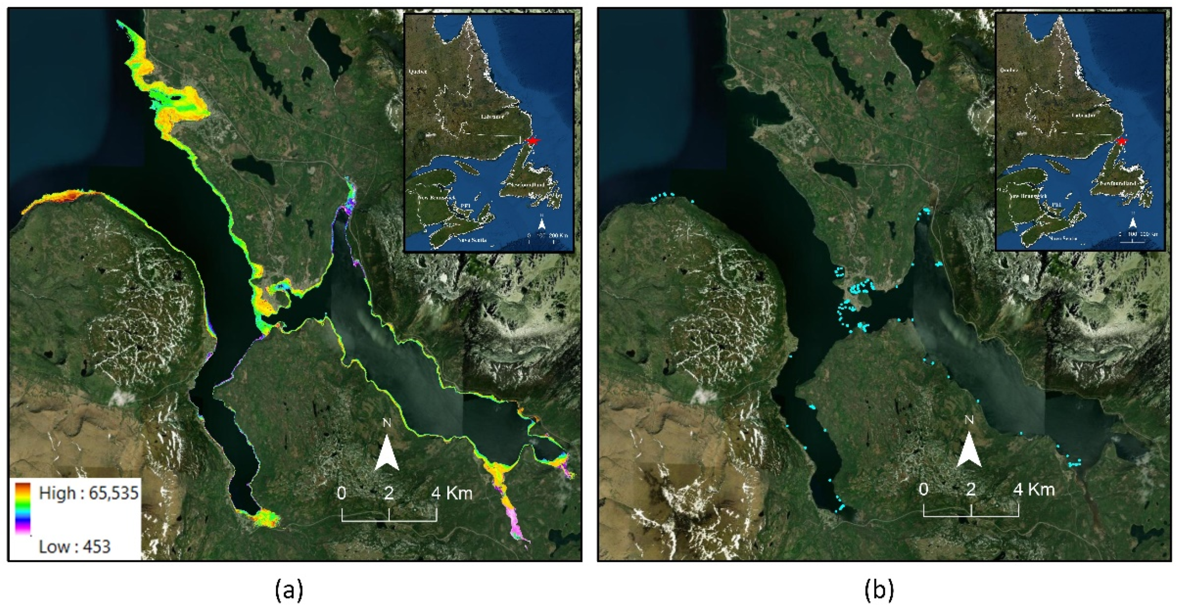
The study area is Bonne Bay (Figure 1a), located on the western side of Newfoundland, Canada (central geographical latitude and longitude are 49°33′ N and 57°55′ W, respectively). Bonne Bay is generally a deep bay with steep nearshore slopes surrounded by steep mountains. It is composed of east and south arms. The east arm comprises an inner basin with a more than 230 m depth, partially separated by a shallow sill (approximately 12 m deep) from the outer bay. The south arm is a shallower basin with a depth of roughly 55 m, fully opening to the Gulf of St. Lawrence [22].
2.2. Field Data
In situ data were collected and provided by Fisheries and Oceans Canada (DFO). Figure 1b demonstrates the distribution of the in situ samples over the study area, and Table 1 provides more information about the number of samples for different marine habitat types. All of the samples were classified based on two different categories: Category 1 had two classes of Vegetation and Non-Vegetation; Category 2 had four classes of Eelgrass, Macroalgae, Fine Sediment, and Gravel/Cobble. Thus, two habitat maps based on Category 1 and Category 2 were produced for this study area.
It is worth noting that after analyzing LiDAR data and investigating high-resolution Google Earth imagery, it was observed that rockweeds could also be identified in the LiDAR data with a high level of accuracy. Thus, Rockweed was also added to the available classes, and several samples for this class were identified by visual interpretation.
2.3. LiDAR Data
The bathymetric LiDAR data were collected by the Canadian Hydrographic Service (CHS). The positional and sounding accuracies of the data have been reported to be 0.1 m and 0.25 m, respectively. Figure 1c illustrates the coverage of the LiDAR data over the water bodies of the study area.
3. Methodology
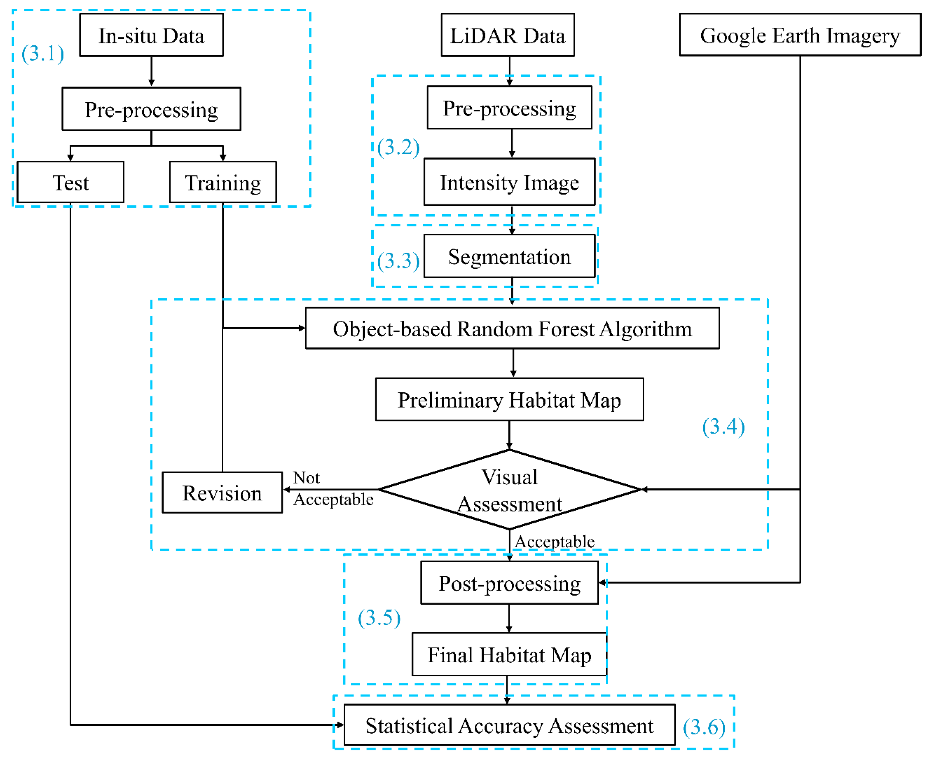
The flowchart of the method to produce the marine habitat map of Bonne Bay using the LiDAR data is illustrated in Figure 2. The detail of each step is also provided below. It should be noted that this flowchart was used to develop two different models to produce two habitat maps based on the Category 1 and Category 2 classes (see Table 1).
3.1. Field Data Preprocessing
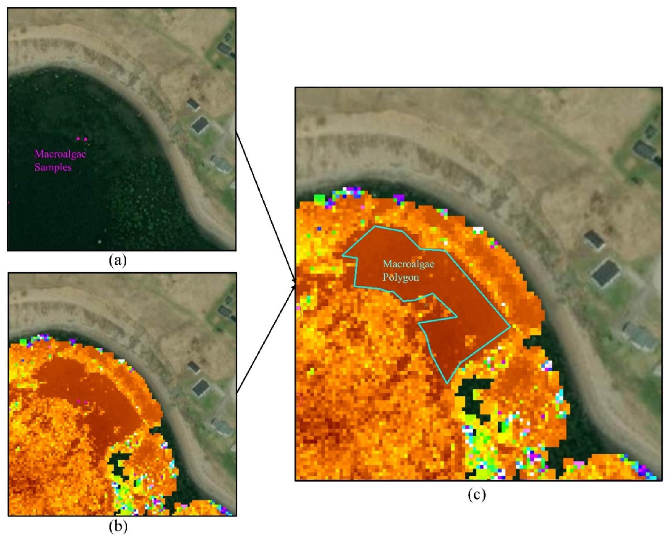
The field samples, which were point-based GPS locations of different habitat types, were inserted into ArcGIS and were converted to polygons where it was possible to do so. To this end, high-resolution Google Earth imagery and the LiDAR intensity product were used. Through this process, the boundary of each homogeneous habitat type at each sample location was delineated. Figure 3 illustrates this procedure for creating a polygon of macroalgae. As it is clear, the intensity values for a macroalgae area were very similar, and they were higher than those of the surrounding pixels. Thus, they belonged to a specific habitat type. By converting field point-based samples to polygons, the number of samples was increased. Finally, all of the polygons were randomly divided into training (70%) and test (30%) data. The training and test polygons were, respectively used for training the machine learning algorithm (see Section 3.4) and an accuracy assessment of the produced marine habitat map (see Section 3.6).
3.2. LiDAR Data Preprocessing
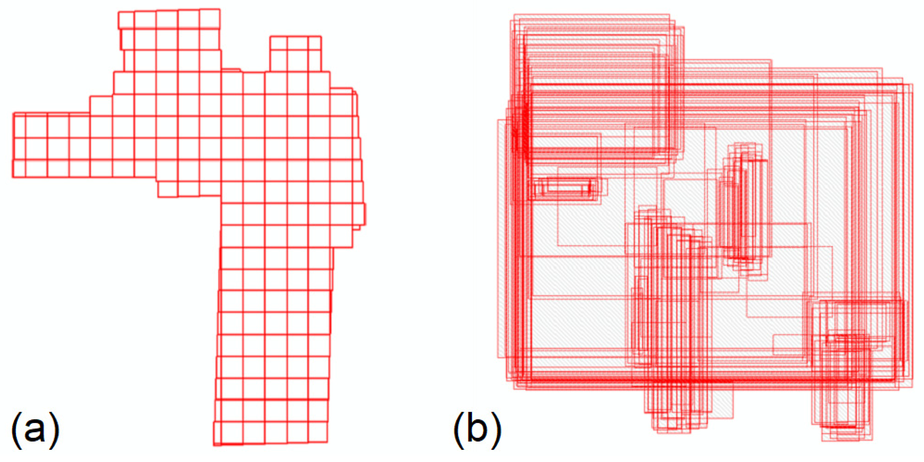
The LiDAR data were provided as three separate groups of LASer (LAS) files: S1, S2, and S3. S1 contained 92 LAS files, while S2 and S3 contained 76 LAS files. The S1 dataset was collected with the LiDAR sensor’s topographic (red) laser, and the other two were collected with the sensor’s bathymetric (green) laser. These two different lasers require different energetic outputs (as penetrating the water column requires more laser energy than penetrating air). The standard post-processing of a LiDAR survey includes the normalization of the returning laser waveforms between the green and red lasers, as well as between the flight lines, and thus, the amplitude of the reflected pulse (i.e., intensity) is consistent and normalized across the entire survey area. After normalization, the waveforms are converted into points, and they are then tiled in a consistent grid format (Figure 4a) that is ready for converting to a raster. The LAS files provided for this study have not undergone these standard post-processing steps, and because the different laser returns were provided separately (S1 vs. S2–S3), flight line artifacts remain throughout the datasets, and the LAS files were not arranged in a consistent grid format (Figure 4b).
In this study, steps were taken to mitigate the lack of standard post-processing during the raster generation process. While this amplitude normalization is not required to derive consistent elevations across a LiDAR survey, it is necessary to produce consistent intensity values across the survey area. For this reason, all three sets of LAS files provided were processed together to produce the Digital Elevation Model (DEM). All LiDAR products were gridded at a spatial resolution of 2 m using a linear interpolation to preserve the integrity of the data while minimizing the data gaps (Figure 5). To remove the land, a mask was made based on land elevation. Through iterative visual analysis, the geomorphic coastline was determined to be roughly 1.8 m in elevation. A buffer of 20 cm elevation was added to this value, and so land over 2 m elevation was removed, and the results were visually checked to ensure no pertinent data were being removed.
To produce the critically important intensity models, the S1 LAS files (a result of the topographic red laser) were processed as one dataset, and the S2–S3 LAS files (results of the bathymetric green laser) were processed as another dataset. Flightline artifacts permeate the intensity dataset (Figure 6), resulting in differing intensity values across homogeneous ground features. Attempts were made to normalize the intensity between the flight lines by comparing the mean intensity of a homogeneous patch of seabed under a flight line divide and applying the mean difference as a linear equation. However, the difference in intensity values varied across the survey area; thus, any corrections in one area enhanced the issues in another area. For this reason, a subsequent analysis was performed using uncorrected gridded intensity data, and separate S1 and S2–S3 intensity raster data.
3.3. Segmentation
It is widely reported that object-based classification methods are more accurate than pixel-based techniques are [8,9,13]. Considering this fact, an object-based classification model was developed in this study to obtain accurate marine habitat maps from the study area. The first step in an object-based image analysis is implementing a segmentation algorithm. In this study, the LiDAR intensity product with a spatial resolution of 2 m was used to segment the study area within the eCognition software package. eCognition provides many toolboxes to implement segmentation and classification, and it usually provides better classification results compared to those produced from commonly used software packages such as ArcGIS and ENVI. In this study, the multiresolution segmentation algorithm available in eCognition was employed. This algorithm merges spectrally similar pixels into segments (objects) with various sizes based on several tuning parameters, such as scale, shape, and compactness [23]. For example, the scale parameter, which is the most important tuning parameter of the multiresolution segmentation algorithm, defines the maximum standard deviation of the homogeneity of the pixels. In this study, the optimum values of these three parameters were selected based on several trial and errors. Finally, the values of 150, 0.4, and 0.5 were selected for the scale, shape, and compactness, respectively.
3.4. Classification
In this study, an RF algorithm was applied to classify the marine habitats. RF had proved higher accuracies compared to other commonly used classification techniques for various applications [24,25]. RF includes a group of decision trees. The final label of a pixel/object is defined based on the votes of the decision trees [26,27]. RF contains two important tuning parameters (i.e., depth and minimum sample number), the optimal values of which should be selected to obtain a high classification accuracy. The depth and minimum sample number, respectively, determine the number of nodes in each tree and the minimum number of samples per node in each tree. In this study, the optimal values of these two parameters were selected based on several trial-and-error attempts, and finally, twenty and five were selected for them, respectively. It should be noted that since object-based image analysis was used in this study, the RF algorithm was applied to the objects produced from the segmentation algorithm. As discussed before, 70% of the field samples were applied to train the RF algorithm. The result of the RF algorithm was the preliminary habitat map which was visually investigated to ensure the accuracy is acceptable. If the result was not satisfactory, the algorithm was refined (e.g., by changing the tuning parameters of the algorithm) to obtain a suitable map.
3.5. Post-Processing
The post-processing step was performed by manually removing any errors and refining the boundaries of some of the classes to improve the produced habitat maps. For example, the maps were compared with the Google Earth imagery near coastlines to see if the aquatic vegetation (e.g., rockweeds) was correctly identified and the errors were removed where it was possible. Moreover, while the machine learning results were acceptable in most parts of the study area, there were several shallow rivers and estuaries where the classification appeared to underestimate the amount of eelgrass. These areas, such as Lomond River, Southeast Arm, and Horseback Brook’s estuary, are environments with significant and complex patches of eelgrass. Many of these eelgrass areas were visually identified in both the imagery and the LiDAR intensity data. After post-processing, the final marine habitat maps were produced.
3.6. Accuracy Assessment
The accuracy of the produced habitat map was assessed using the test data (i.e., 30% of the independent field samples) to obtain the classification accuracy level. To this end, the confusion matrix of the classification was generated, and several accuracy indices, such as overall accuracy, kappa coefficient, and producer and user accuracies were evaluated. It is worth noting that the statistical accuracy assessment was performed before and after the post-processing step to evaluate the accuracies of both developed RF model and the final refined habitat map, respectively.
4. Results and Discussion
The method described in Section 3 was applied to produce two marine habitat maps based on the classes described in Table 1: a two-class habitat map (Category 1) and a five-class habitat map (Category 2). In the following two subsections, the corresponding maps and the accuracy levels are provided.
4.1. Two-Class Habitat Map (Category-1)
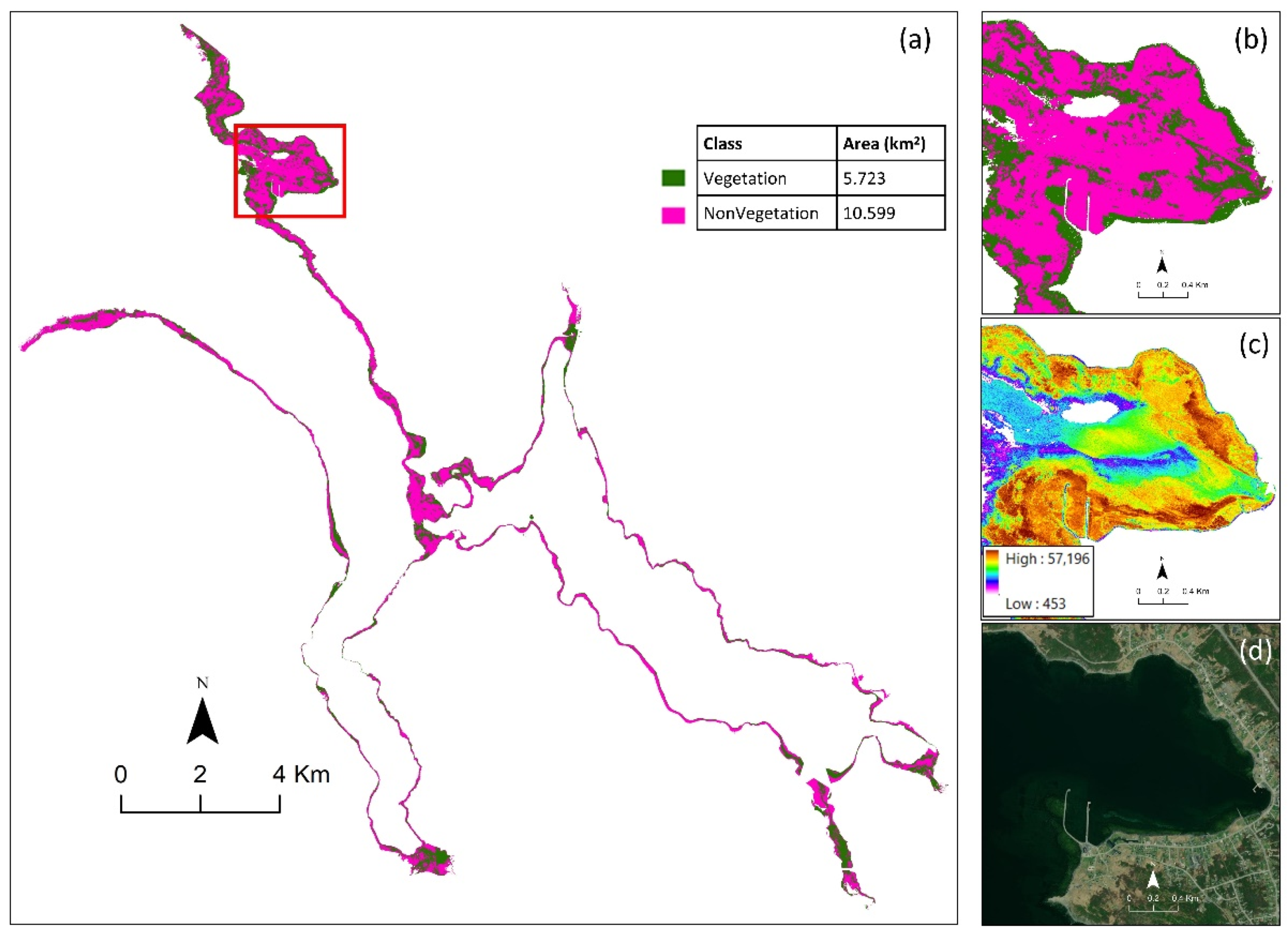
Figure 7 shows the classified habitat map based on the Category 1 classes obtained from the object-based RF algorithm. First, the accuracy of this map was visually investigated by comparing it with high-resolution Google Earth images and LiDAR intensity products. The identified areas had a good correlation with the real Vegetation and Non-Vegetation areas. The areas of the classes were also calculated, and the results are reported in Figure 7. Vegetation and Non-vegetation cover approximately 5.7 km2 (35%) and 10.6 km2 (65%) of the study area, respectively.
The accuracy of the produced habitat map based on the Category 1 classes was also assessed using the confusion matrix, where the results are provided in Table 2. The overall accuracy was 87%, indicating the high potential of the developed technique for discriminating the Vegetation and Non-Vegetation classes in Bonne Bay. This level of overall accuracy simply means that if we randomly select 100 points pixels of 2 × 2 m considering both classes, 87 of them would be accurately identified within the produced map.
The producer and user accuracies along with the omission and commission errors for each class of Vegetation and Non-Vegetation are also provided in Table 2. The producer accuracies for both classes and user accuracy for the Vegetation class were high (between 85% and 92%). However, the user accuracy of the non-Vegetation class was relatively low (~79%). This means that there were some Vegetation samples that were wrongly classified as the Non-Vegetation class (high commission error). This can be easily seen in the confusion matrix where 690 pixels of Vegetation (out of 3255 pixels) were incorrectly classified as Non-Vegetation.
The accuracy assessment of the classification model for the two-class habitat mapping was also assessed before post-processing, and it was observed that post-processing did not significantly affect the accuracy assessment. In this case, the overall accuracy and kappa coefficient were 87% and 0.69, respectively.
4.2. Five-Class Habitat Map (Category-2)
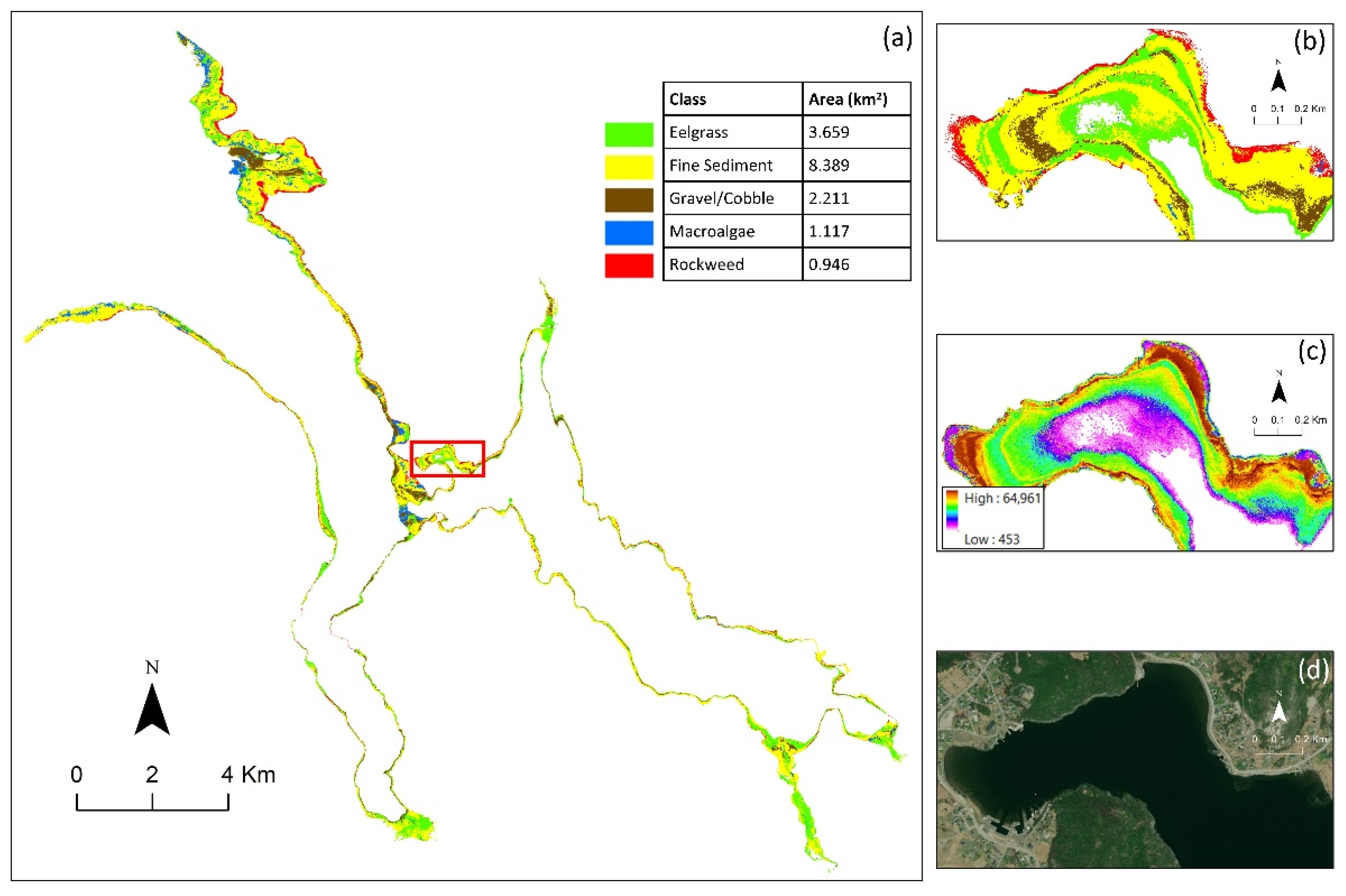
Figure 8 illustrates the habitat map based on the Category 2 classes. First, the accuracy of this map was visually assessed using high-resolution Google Earth images and the LiDAR intensity product, and it was observed that the map was visually accurate. The areas of the classes were also calculated from this map (see Figure 8). The results showed that the Fine Sediment class had the highest coverage (8.4 km2). The smallest coverage also belonged to the Rockweed and Macroalgae classes, which cover 0.95 km2 (5.8%) and 1.1 km2 (6.8%) of the study area, respectively.
The confusion matrix of the five-class habitat map, which shows the overall accuracy and class accuracies, is provided in Table 3. The overall accuracy and kappa coefficients were 80% and 0.7, respectively, which were reasonable considering that there were several challenges during this project. Overall, based on both producer and user accuracies, Rockweed had the highest accuracies (producer accuracy = 88%, user accuracy = 99%), which was followed by Gravel/Cobble (producer accuracy = 74%, user accuracy = 85%) and Eelgrass (producer accuracy = 86%, user accuracy = 64%). For example, 3958 pixels of the in situ Rockweed samples (out of 4492 pixels) were correctly classified as Rockweed. The lowest accuracies (highest commission and omission errors) were observed for the Macroalgae class (producer accuracy = 44%, user accuracy = 58%). The main reason for this was that a large portion of the Macroalgae samples (95 pixels out of 226 pixels) were wrongly classified as Fine Sediment. There was also some confusion between this class with the Rockweed class, where 31 pixels of Macroalgae were incorrectly classified as Rockweed. Another high confusion was also observed between Fine Sediment and other classes. For instance, 378 in situ pixels of the Fine Sediment (27%) were wrongly classified as Eelgrass. Overall, there was an overestimation of Fine Sediment because there were many in situ samples from other classes which were incorrectly classified as Fine Sediment.
The accuracy assessment of the classification model for the five-class habitat mapping was also assessed before post-processing. In this case, the overall accuracy and kappa coefficient were 76% and 0.68, respectively. Thus, the post-processing step slightly improved the classification result of the five-class habitat map.
4.3. Limitations and Suggestions
In this project, LiDAR data along with a machine learning model were applied to classify the marine habitats in Bonne Bay, Newfoundland. The results showed the potential of the proposed method for habitat classification in other marine areas. Below, the main limitations of the project along with several suggestions are provided to improve the results in future works.
As discussed in Section 2.3, although several efforts were made to remove the errors of the LiDAR raw data, some of these errors could not be resolved through the post-processing steps. This would negatively affect the results of any studies which utilize similar datasets.
Although the collected in situ data were beneficial to obtain reasonable habitat maps, more samples are required to develop a more accurate and robust machine learning model. For example, the number of samples of the Macroalgae class was very low. In fact, this was one of the main reasons for the low accuracy of this class in the produced map (see Figure 8 and Table 3). Overall, a higher number of samples provides a higher classification accuracy in a machine learning model.
One approach to improve the classification results is by utilizing other types of remote sensing datasets, such as very high resolution optical satellites and drone imagery. These imageries would provide valuable information about marine habitats, especially over shallower water areas. Additionally, high-resolution satellite images are very beneficial when the objective is mapping and changing the analysis of marine habitats at regional and global scales.
5. Conclusions
Marine habitats provide many services to both the marine ecosystem and humans, and therefore, they should be accurately monitored using advanced technologies. In this regard, airborne bathymetric LiDAR systems have great advantages for oceanographic applications, such as bathymetric mapping and marine habitat classification. Bathymetric LiDAR pulses can penetrate into water and can identify different marine habitats based on the intensity values. This study used bathymetric LiDAR data to accurately discriminate five habitat types of Eelgrasses, Macroalgae, Rockweed, Fine Sediment, and Gravel/Cobble using LiDAR intensity data. It was observed that LiDAR data has a great potential to discriminate the Vegetation from the Non-Vegetation classes in marine environments. For example, the overall classification accuracy for distinguishing these two classes was 87%. Moreover, the accuracy of the five-class habitat map was reasonably accurate (overall accuracy = 80%). It was concluded that the LiDAR data could identify the Rockweed class with the highest accuracy (e.g., producer and user accuracies were 88% and 99%, respectively). However, the accuracy of identifying the Macroalgae class was relatively low. The main reason for this was the lack of in situ data for this class in our study. Additionally, Macroalgae is usually found in deeper water compared to other aquatic vegetation species, and thus, it can be identified with a lower accuracy using LiDAR data. In summary, lacking enough in situ samples for some of the classes and the errors of the LiDAR data were the main limitations of this study to obtain a better classification accuracy. Therefore, future studies should employ more balanced in situ data and very high resolution satellite and drone imagery along with better LiDAR data to achieve a more classification accuracy. Finally, the proposed method should be applied to other study areas to investigate its robustness at different conditions. In this regard, the effects of water quality and climate conditions on the LiDAR pulses, and consequently, on the classification results could be investigated further.
Author Contributions
Conceptualization, M.A.; Data curation, M.A., C.M. and S.M.; Formal analysis, M.A., C.M. and S.M.; Funding acquisition, M.A. and M.G.; Investigation, M.A. and C.M.; Methodology, M.A. and C.M.; Resources, M.A.; Software, M.A. and C.M.; Supervision, M.A.; Validation, M.A. and C.M.; Visualization, M.A. and C.M.; Writing—original draft, M.A., C.M. and A.S.; Writing—review and editing, M.A., C.M., A.S., S.M. and M.G. All authors have read and agreed to the published version of the manuscript.
Funding
This research received no external funding.
Data Availability Statement
Not applicable.
Acknowledgments
The authors thank David Forsey, Philip Sargent, and Kyle Matheson from Fisheries and Oceans Canada (NAFC, St. John’s, NL, Canada) for their valuable input during the project.
Conflicts of Interest
The authors declare no conflict of interest.
References
- Amani, M.; Ghorbanian, A.; Asgarimehr, M.; Yekkehkhany, B.; Moghimi, A.; Jin, S.; Naboureh, A.; Mohseni, F.; Mahdavi, S.; Layegh, N. Remote Sensing Systems for Ocean: A Review (Part 1: Passive Systems). IEEE J. Sel. Top. Appl. Earth Obs. Remote Sens. 2022, 15, 210–234. [Google Scholar] [CrossRef]
- Amani, M.; Mohseni, F.; Layegh, N.F.; Nazari, M.E.; Fatolazadeh, F.; Salehi, A.; Ahmadi, S.A.; Ebrahimy, H.; Ghorbanian, A.; Jin, S.; et al. Remote Sensing Systems for Ocean: A Review (Part 2: Active Systems). IEEE J. Sel. Top. Appl. Earth Obs. Remote Sens. 2022, 15, 1421–1453. [Google Scholar] [CrossRef]
- Amani, M.; Moghimi, A.; Mirmazloumi, S.M.; Ranjgar, B.; Ghorbanian, A.; Ojaghi, S.; Ebrahimy, H.; Naboureh, A.; Nazari, M.E.; Mahdavi, S.; et al. Ocean Remote Sensing Techniques and Applications: A Review (Part I). Water 2022, 14, 3400. [Google Scholar] [CrossRef]
- Amani, M.; Mehravar, S.; Asiyabi, R.M.; Moghimi, A.; Ghorbanian, A.; Ahmadi, S.A.; Ebrahimy, H.; Moghaddam, S.H.A.; Naboureh, A.; Ranjgar, B.; et al. Ocean Remote Sensing Techniques and Applications: A Review (Part II). Water 2022, 14, 3401. [Google Scholar] [CrossRef]
- Custodio, M.; Moulaert, I.; Asselman, J.; van der Biest, K.; van de Pol, L.; Drouillon, M.; Lucas, S.H.; Taelman, S.E.; Everaert, G. Prioritizing ecosystem services for marine management through stakeholder engagement. Ocean Coast. Manag. 2022, 225, 106228. [Google Scholar] [CrossRef]
- Oliveira; Silva, L.O.; Resende, M.; Galhardas, H.; Manquinho, V.; Lynce, I. DeepData: Machine learning in the marine ecosystems. Expert Syst. Appl. 2022, 206, 117841. [Google Scholar] [CrossRef]
- Wedding, L.; Friedlander, A.; McGranaghan, M.; Yost, R.; Monaco, M. Using bathymetric lidar to define nearshore benthic habitat complexity: Implications for management of reef fish assemblages in Hawaii. Remote Sens. Environ. 2008, 112, 4159–4165. [Google Scholar] [CrossRef]
- Copertino, M.S.; Creed, J.C.; Lanari, M.O.; Magalhães, K.; Barros, K.; Lana, P.C.; Sordo, L.; Horta, P.A. Seagrass and Submerged Aquatic Vegetation (VAS) Habitats off the Coast of Brazil: State of knowledge, conservation and main threats. Braz. J. Oceanogr. 2016, 64, 53–80. [Google Scholar] [CrossRef]
- Janauer, G.A. Aquatic Vegetation in River Floodplains: Climate Change Effects, River Restoration and Ecohydrology Aspects. Clim. Chang. Inferences Paleoclim. Reg. Asp. 2012, 149–155. [Google Scholar] [CrossRef]
- Trebilco, R.; Fleming, A.; Hobday, A.J.; Melbourne-Thomas, J.; Meyer, A.; McDonald, J.; Pecl, G.T. Warming world, changing ocean: Mitigation and adaptation to support resilient marine systems. Rev. Fish Biol. Fish. 2021, 32, 39–63. [Google Scholar] [CrossRef]
- White, E.; Amani, M.; Mohseni, F. Coral Reef Mapping Using Remote Sensing Techniques and a Supervised Classification Algorithm. Adv. Environ. Eng. Res. 2021, 2, 1. [Google Scholar] [CrossRef]
- Amani, M.; Macdonald, C.; Mahdavi, S.; Gullage, M.; So, J. Aquatic Vegetation Mapping Using Machine Learning Algorithms And Bathymetric Lidar Data: A Case Study From Newfoundland, Canada. J. Ocean Technol. 2021, 16, 76–94. [Google Scholar]
- Collin, A.; Archambault, P.; Long, B. Predicting species diversity of benthic communities within turbid nearshore using full-waveform bathymetric LiDAR and machine learners. PLoS ONE 2011, 6, 21265. [Google Scholar] [CrossRef] [Green Version]
- Chust, G.; Grande, M.; Galparsoro, I.; Uriarte, A.; Borja, Á. Capabilities of the bathymetric Hawk Eye LiDAR for coastal habitat mapping: A case study within a Basque estuary. Estuar. Coast. Shelf Sci. 2010, 89, 200–213. [Google Scholar] [CrossRef]
- Zavalas, R.; Ierodiaconou, D.; Ryan, D.; Rattray, A.; Monk, J. Habitat classification of temperate marine macroalgal communities using bathymetric LiDAR. Remote Sens. 2014, 6, 2154–2175. [Google Scholar] [CrossRef] [Green Version]
- Mohseni, F.; Saba, F.; Mirmazloumi, S.M.; Amani, M.; Mokhtarzade, M.; Jamali, S.; Mahdavi, S. Ocean water quality monitoring using remote sensing techniques: A review. Mar. Environ. Res. 2022, 180, 105701. [Google Scholar] [CrossRef]
- Webster, T.; McGuigan, K.; Collins, K.; Crowell, N.; MacDonald, C. Evaluating a Topo-Bathymetric Lidar Sensor to Map Submerged Aquatic Vegetation in Lake Banook. Technical Report, Applied Geomatics Research Group, NSCC Middleton, NS. Available online: https://agrg.cogs.nscc.ca/dl/reports/2015/2015_Topo-Bathymetric_Lidar_to_Map_SAV_Lake_Banook.pdf (accessed on 11 November 2022).
- Webster, T.; MacDonald, C.; McGuigan, K.; Crowell, N.; Lauzon-Guay, J.S.; Collins, K. Calculating macroalgal height and biomass using bathymetric LiDAR and a comparison with surface area derived from satellite data in Nova Scotia, Canada. Bot. Mar. 2020, 63, 43–59. [Google Scholar] [CrossRef]
- Letard, M.; Collin, A.; Lague, D.; Corpetti, T.; Pastol, Y.; Ekelund, A.; Costa, S. Towards 3D mapping of seagrass meadows with topo-bathymetric lidar full waveform processing. In Proceedings of the 2021 IEEE International Geoscience and Remote Sensing Symposium IGARSS, Brussels, Belgium, 11–16 July 2021; pp. 8069–8072. [Google Scholar]
- Letard, M.; Collin, A.; Corpetti, T.; Lague, D.; Pastol, Y.; Ekelund, A. Classification of Land-Water Continuum Habitats Using Exclusively Airborne Topobathymetric Lidar Green Waveforms and Infrared Intensity Point Clouds. Remote Sens. 2022, 14, 341. [Google Scholar] [CrossRef]
- Smith, G.; Yesilnacar, E.; Jiang, J.; Taylor, C. Marine habitat mapping incorporating both derivatives of LiDAR data and hydrodynamic conditions. J. Mar. Sci. Eng. 2015, 3, 492–508. [Google Scholar] [CrossRef] [Green Version]
- Quijón, P.A.; Snelgrove, P.V.R. Predation regulation of sedimentary faunal structure: Potential effects of a fishery-induced switch in predators in a Newfoundland sub-Arctic fjord. Oecologia 2005, 144, 125–136. [Google Scholar] [CrossRef]
- Baatz, M.; Schape, A. Multiresolution Segmentation: An Optimization Approach for High Quality Multi-Scale Image Segmentation. In Proceedings of the Angewandte Geographische Informations Verarbeitung XII; Wichmann Verlag: Karlsruhe, Germany, 2000; pp. 12–23. [Google Scholar]
- Amani, M.; Salehi, B.; Mahdavi, S.; Granger, J.; Brisco, B. Wetland classification in Newfoundland and Labrador using multi-source SAR and optical data integration. GISci. Remote Sens. 2017, 54, 779–796. [Google Scholar] [CrossRef]
- Mahdavi, S.; Salehi, B.; Amani, M.; Granger, J.E.; Brisco, B.; Huang, W.; Hanson, A. Object-Based Classification of Wetlands in Newfoundland and Labrador Using Multi-Temporal PolSAR Data. Can. J. Remote Sens. 2017, 43, 432–450. [Google Scholar] [CrossRef]
- Belgiu, M.; Drăguţ, L. Random forest in remote sensing: A review of applications and future directions. ISPRS J. Photogramm. Remote Sens. 2016, 114, 24–31. [Google Scholar] [CrossRef]
- Sheykhmousa, M.; Mahdianpari, M.; Ghanbari, H.; Mohammadimanesh, F.; Ghamisi, P.; Homayouni, S. Support Vector Machine Versus Random Forest for Remote Sensing Image Classification: A Meta-Analysis and Systematic Review. IEEE J. Sel. Top. Appl. Earth Obs. Remote Sens. 2020, 13, 6308–6325. [Google Scholar] [CrossRef]
Figure 1.
(a) Coverage of the LiDAR data (the image shows the intensity values), (b) distribution of the in situ samples over the study area. The red star indicates the location of the study area (i.e., Bonne Bay in Newfoundland, Canada).
Figure 1.
(a) Coverage of the LiDAR data (the image shows the intensity values), (b) distribution of the in situ samples over the study area. The red star indicates the location of the study area (i.e., Bonne Bay in Newfoundland, Canada).

Figure 2.
The flowchart of the classification model for marine habitat mapping.

Figure 3.
The procedure of converting the in situ sample points to the GIS polygons: (a) two in situ samples of Macroalgae overlaid on the high-resolution Google Earth imagery; (b) the same region in the LiDAR intensity image; (c) the generated polygon for these two samples in the ArcGIS software.
Figure 3.
The procedure of converting the in situ sample points to the GIS polygons: (a) two in situ samples of Macroalgae overlaid on the high-resolution Google Earth imagery; (b) the same region in the LiDAR intensity image; (c) the generated polygon for these two samples in the ArcGIS software.

Figure 4.
(a) A typical LAS dataset after undergoing standard post-processing; (b) the LAS dataset produced from each of the S1, S2, and S3 groups of LAS files provided from CHS.
Figure 4.
(a) A typical LAS dataset after undergoing standard post-processing; (b) the LAS dataset produced from each of the S1, S2, and S3 groups of LAS files provided from CHS.

Figure 5.
(a,b) show 1 m elevation data for S2–S3 datasets, while (c,d) shows the same data but gridded at 2 m to minimize data gaps.
Figure 5.
(a,b) show 1 m elevation data for S2–S3 datasets, while (c,d) shows the same data but gridded at 2 m to minimize data gaps.

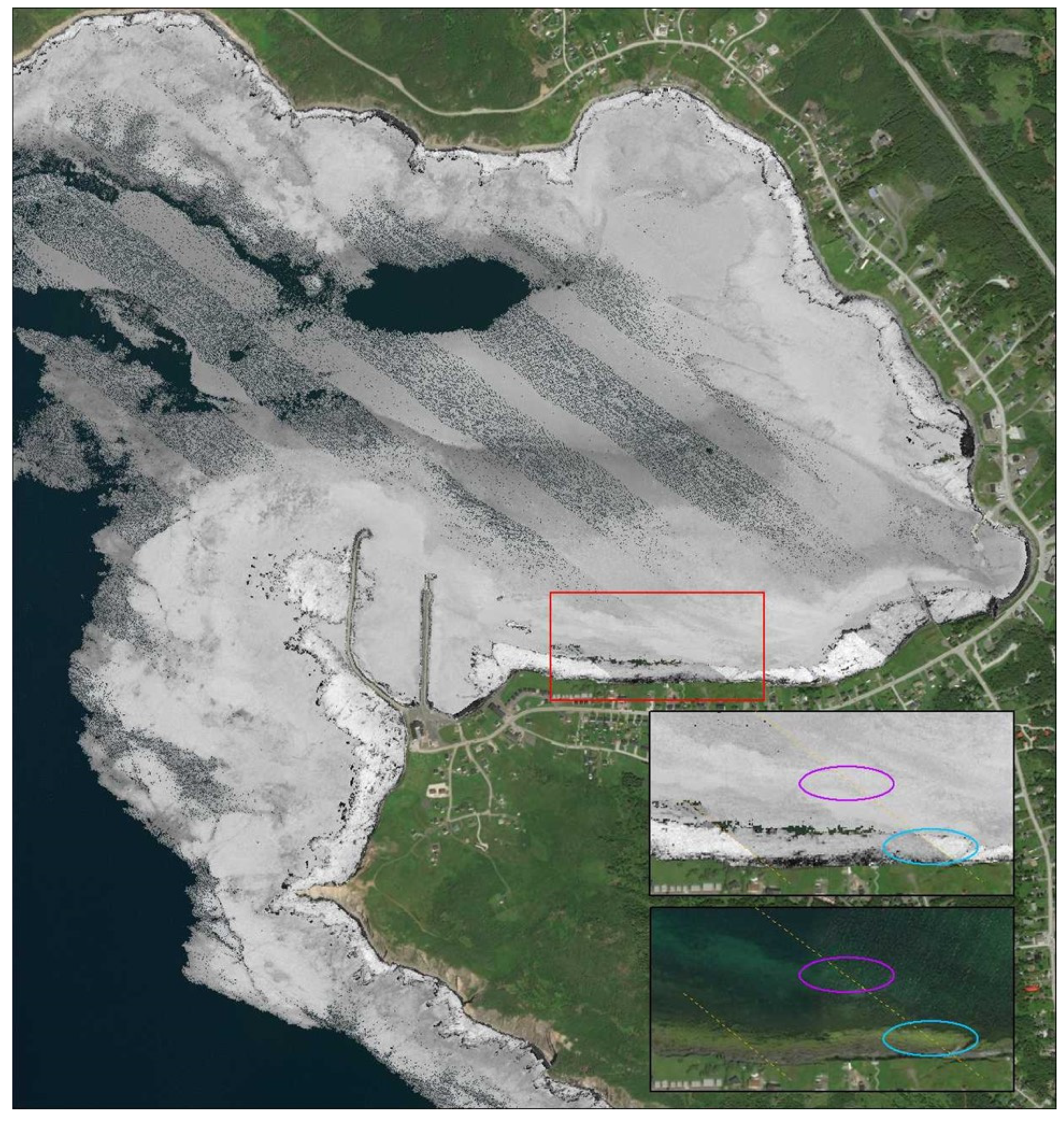
Figure 6.
Flightline artifacts (striping) can be seen throughout the 2 m intensity data. The insets (red box) show the differing intensities between flight lines for homogeneous ground features such as rockweed (blue ellipse) and sediment (purple ellipse).
Figure 6.
Flightline artifacts (striping) can be seen throughout the 2 m intensity data. The insets (red box) show the differing intensities between flight lines for homogeneous ground features such as rockweed (blue ellipse) and sediment (purple ellipse).

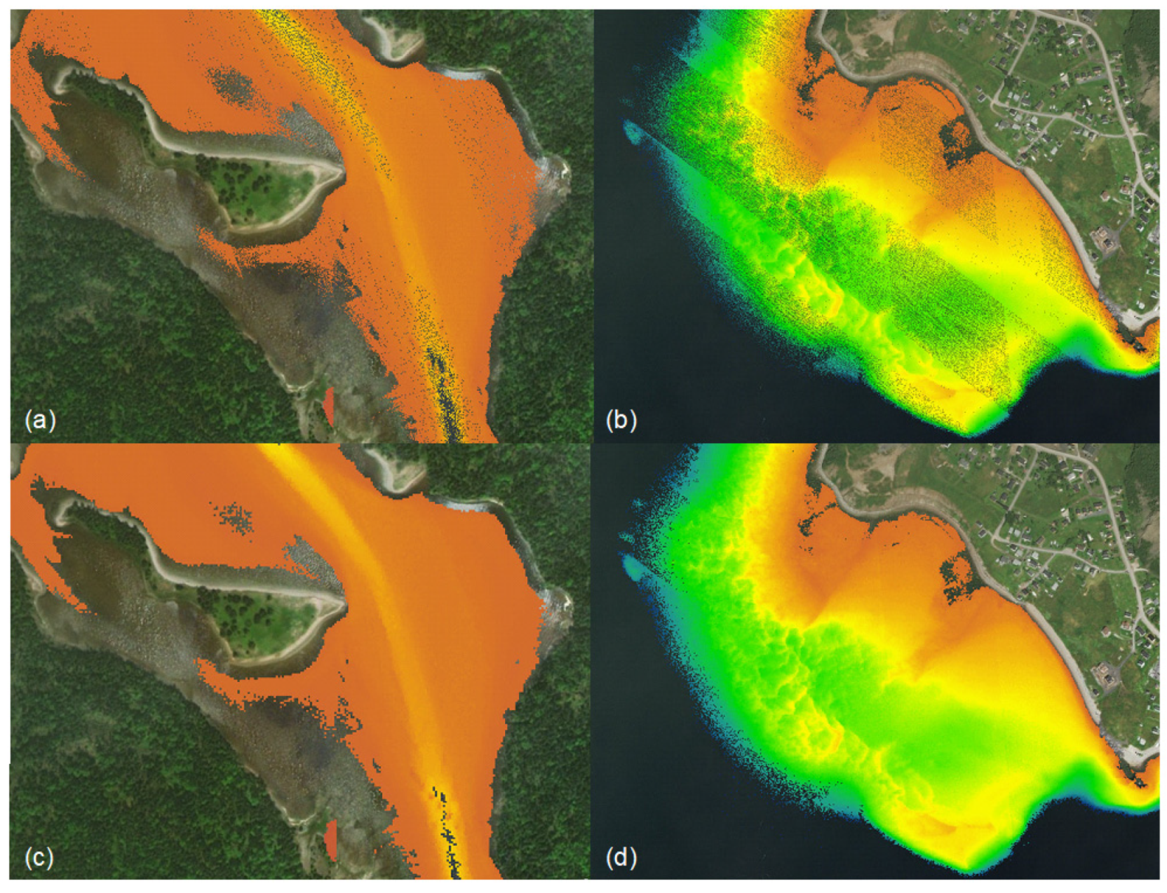
Figure 7.
(a) Habitat map of Bonne Bay based on the Category 1 classes. (b) A zoomed area (red boundary in (a)) from the map along with the (c) LiDAR intensity image and (d) very high-resolution Google Earth imagery to demonstrate the visual accuracy of the map.
Figure 7.
(a) Habitat map of Bonne Bay based on the Category 1 classes. (b) A zoomed area (red boundary in (a)) from the map along with the (c) LiDAR intensity image and (d) very high-resolution Google Earth imagery to demonstrate the visual accuracy of the map.

Figure 8.
(a) Habitat map of Bonne Bay based on the Category-2 classes. (b) A zoomed area (red boundary in (a)) from the map along with the (c) LiDAR intensity image and (d) very high-resolution Google Earth imagery to demonstrate the visual accuracy of the map.
Figure 8.
(a) Habitat map of Bonne Bay based on the Category-2 classes. (b) A zoomed area (red boundary in (a)) from the map along with the (c) LiDAR intensity image and (d) very high-resolution Google Earth imagery to demonstrate the visual accuracy of the map.


Table 1.
The number of in situ samples for different habitat types.
| Category 1 | Category 2 | Number of Samples |
|---|---|---|
| Vegetation | Eelgrass | 27 |
| Macroalgae | 10 | |
| Rockweed * | 8 | |
| Non-Vegetation | Fine Sediment | 53 |
| Gravel/Cobble | 36 |
Note: * The samples for the Rockweed class were identified by visual interpretation of the high-resolution Google Earth imagery.
Table 2.
Confusion matrix of the classification based on the Category 1 classes.
| In Situ Data | ||||||
|---|---|---|---|---|---|---|
| Vegetation | Non-Vegetation | Total | User Accuracy (%) | Commission Error (%) | ||
| Classified | Vegetation | 4925 | 444 | 5369 | 91.7 | 8.3 |
| Non-Vegetation | 690 | 2565 | 3255 | 78.8 | 21.2 | |
| Total | 5615 | 3009 | 8624 | |||
| Producer Accuracy (%) | 87.7 | 85.24 | Overall Accuracy = 87% | |||
| Omission Error (%) | 12.3 | 14.76 | Kappa Coefficient = 0.71 | |||
Table 3.
Confusion matrix of the classification based on the Category 2 classes.
| In situ Data | |||||||||
|---|---|---|---|---|---|---|---|---|---|
| Eelgrass | Gravel/Cobble | Fine Sediment | Macroalgae | Rockweed | Total | User Accuracy (%) | Commission Error (%) | ||
| Classified | Eelgrass | 774 | 55 | 378 | 0 | 0 | 1207 | 64.1 | 35.9 |
| Gravel/Cobble | 44 | 1175 | 159 | 0 | 5 | 1383 | 85.0 | 15.0 | |
| Fine Sediment | 78 | 355 | 876 | 95 | 468 | 1872 | 46.8 | 53.2 | |
| Macroalgae | 1 | 2 | 9 | 100 | 61 | 173 | 57.8 | 42.2 | |
| Rockweed | 0 | 0 | 0 | 31 | 3958 | 3989 | 99.2 | 0.8 | |
| Total | 897 | 1587 | 1422 | 226 | 4492 | 8624 | |||
| Producer Accuracy (%) | 86.3 | 74.0 | 61.6 | 44.2 | 88.1 | Overall Accuracy = 80% | |||
| Omission Error (%) | 13.7 | 26.0 | 38.4 | 55.8 | 11.9 | Kappa Coefficient = 0.7 | |||
Publisher’s Note: MDPI stays neutral with regard to jurisdictional claims in published maps and institutional affiliations. |
© 2022 by the authors. Licensee MDPI, Basel, Switzerland. This article is an open access article distributed under the terms and conditions of the Creative Commons Attribution (CC BY) license (https://creativecommons.org/licenses/by/4.0/).
Share and Cite
MDPI and ACS Style
Amani, M.; Macdonald, C.; Salehi, A.; Mahdavi, S.; Gullage, M. Marine Habitat Mapping Using Bathymetric LiDAR Data: A Case Study from Bonne Bay, Newfoundland. Water 2022, 14, 3809. https://doi.org/10.3390/w14233809
AMA Style
Amani M, Macdonald C, Salehi A, Mahdavi S, Gullage M. Marine Habitat Mapping Using Bathymetric LiDAR Data: A Case Study from Bonne Bay, Newfoundland. Water. 2022; 14(23):3809. https://doi.org/10.3390/w14233809
Chicago/Turabian StyleAmani, Meisam, Candace Macdonald, Abbas Salehi, Sahel Mahdavi, and Mardi Gullage. 2022. "Marine Habitat Mapping Using Bathymetric LiDAR Data: A Case Study from Bonne Bay, Newfoundland" Water 14, no. 23: 3809. https://doi.org/10.3390/w14233809
Note that from the first issue of 2016, this journal uses article numbers instead of page numbers. See further details here.