Inundation Characteristics of Solitary Waves According to Revetment Type

Abstract

Wave absorbers installed in front of revetments are effective in reducing wave overtopping and inundation caused by periodic waves. The wave absorbers’ mechanism of reducing wave overtopping and inundation caused by long-period waves such as tsunamis and storm surges is not clearly understood. This study conducted a physical modeling test and numerical analysis based on a large eddy simulation model using in-house code to examine the characteristics of wave overtopping and inundation according to the revetment type for solitary waves. In a vertical revetment (VR), the dominant vertical velocity of the solitary wave cannot bend at a right angle during overtopping, causing flow separation to occur at the crest, which leads to increased drag and vorticity. In a wave absorbing revetment (WAR), the flow cross-sectional area decreases along the slope of the wave absorber, causing the flow velocity of the solitary wave to increase and the horizontal velocity to be dominant during the overtopping and inundation process. In contrast with the general wave overtopping characteristics of periodic waves, the maximum overtopping water surface elevation in front of the vertical wall is higher in a VR than in a WAR. However, the order of maximum inundation heights reverses as the wave propagates inland.

1. Introduction

The 2004 Indian Ocean earthquake of magnitude 9.1 and the related tsunami resulted in the most severe casualties from an earthquake recorded to date. In 10 countries across South Asia and East Africa, the disaster resulted in over 283,100 deaths, 14,100 missing, and 1,126,900 displaced people. Most of the deaths were due to the inundation process caused by wave overtopping from the tsunami. Additionally, the Fukushima nuclear plant was damaged by the 9.1-magnitude 2011 Tohoku earthquake and tsunami. As the tsunami inundated the Fukushima nuclear plant, emergency generators and coolant intake pumps became unusable, leading to a meltdown and explosions, thus exposing the surrounding area to radiation. The plant is still in the process of restoration and does not have a definite restoration timeline. The International Atomic Energy Agency designated this as a Level 7 (major) accident, which is the highest risk designation on the International Nuclear and Radiological Event Scale and is the same as that of the 1986 Chernobyl disaster.

The direct damage by a tsunami is caused by a process that leads to shockwaves, run-up, wave overtopping, and inundation. Hence, researchers have actively studied shoaling and run-up by applying solitary waves or tsunami-like waves rather than tsunamis in coastal areas [1,2,3,4,5,6]. There have also been numerous theoretical [7], experimental [6], and numerical [8,9,10,11,12,13] studies on the overtopping of tsunami-like waves or solitary waves formed from run-up.

Most studies on tsunami inundation involve physical modeling tests and numerical analysis applied to coastal cities or fringing reefs. Rueben et al. [14] conducted a representative study by considering coastal cities, built a 1/50-scale model of the town of Seaside, Oregon, USA, in a large tank, and reported that macro-roughness introduced by elements such as structures and houses reduces the bore speed by 40% when a tsunami-like wave passes over them. Additionally, Shin et al. [15] and Park et al. [16] conducted a numerical analysis by applying the experimental conditions of Rueben et al. [14]; as in the experiment, the maximum momentum flux occurred near the shoreline and decreased as it moved inland. Shin et al. [15] represented the coastal city three-dimensionally in a 3D large eddy simulation (LES) model based on the Navier–Stokes (NS) equation, which can analyze a two-phase flow. Park et al. [16] used COULWAVE [17,18,19], a depth-integrated numerical model based on the Boussinesq equation that can account for the bottom-stress-driven turbulence effect, to study the inundation height, flow velocity, and momentum flux according to the coefficient of friction. Prasetyo et al. [20] used a 1/250-scale physical model, 2D nonlinear shallow-water equation model, and quasi-three-dimensional model and found that the effects of macro-roughness on tsunami inundation in the town of Onagawa, Miyagi Prefecture, Japan, when the 2011 Tohoku tsunami passed, were similar to those reported in previous studies. Yasuda et al. [21] recognized the necessity to accurately predict tsunami inundation and compared and reviewed various numerical model results with the 1/250-scale physical modeling results of Prasetyo et al. [20]. They experimented with a 1/250-scale model and confirmed that, in a complex urban area such as the town of Onagawa, the resolution of the topographic data is an important parameter in the inundation analysis and suggested a topographic resolution of 1 cm intervals as a sufficient condition by considering the computational cost and accuracy.

Revetments and levees are constructed on coasts to protect life and property (land and structures) from ocean forces such as waves and tides. Initially, nearly vertical impermeable structures such as stone walls were installed on coasts to protect the foundation from ocean forces. Recently, however, with the development of various wave-absorbing blocks, wave dissipation methods have also been applied to protect the coasts from wave overtopping. As for recent research trends on wave overtopping, various studies are considering the response to climate change, eco-friendliness, and advanced technology. Wave overtopping studies using physical modeling test considered introducing artificial coral reefs to existing structures, providing eco-friendly and biological advances to improve climate change resilience [22,23]. Various retrofitting structures (diffraction pillars, reef breakwaters, vegetation, and recurve walls) were investigated to reduce wave overtopping [24,25], considering climate change resilience. In addition, Dong et al. analyzed wave impact pressure and overturning moment generated from the wave impact force by applying a retrofitting recurve wall to evaluate the safety of the structure and wave overtopping reduction of the structure with retrofitting [26]. Furthermore, studies were conducted to quantify the wave-by-wave overtopping volume [27] and to analyze the spatial distribution of the overtopping discharge behind the structure [28]. For the numerical modeling, as the utility of the smoothed particle hydrodynamics model has recently increased in the field of coastal marine engineering, it is being applied to the calculation of wave overtopping, impact, and runoff [29,30]. However, most wave overtopping studies have focused on periodic waves; even the EurOtop guideline, which contains numerous research results on wave overtopping, has limited information on the reduction effects of the wave dissipation methods in wave overtopping and inundation of bores and long-period waves such as tsunamis [31,32].

Lee et al. [33] conducted physical modeling and numerical analysis of the overtopping of solitary waves in vertical revetments (VRs) and wave-absorbing revetments (WARs). They demonstrated that for a high wave, the overtopping rate of the VR was less than that of the WAR, owing to the effect of the wave absorber. However, they reported that under the condition $\epsilon \left(A/h\right)<0.272$, the overtopping rate of the WAR was greater than that of the VR (here, $A$ is the solitary wave amplitude and $h$ is the depth). For such a VR or WAR, overtopping of the solitary wave leads to land inundation. Unfortunately, as Lee et al. [33] measured the overtopping rate in a tank installed on land, their findings have many limitations in the understanding of the inundation characteristics of solitary waves. Since phenomena such as run-up, wave overtopping, and flooding that occur in the coast directly affect property damage, it is necessary to clearly analyze the characteristics of inundation in the land area according to the revetment type.

In this study, the inundation of solitary waves in VR and WAR was analyzed using experimental and numerical methods. First, VR and WAR were installed in separate experimental tanks; the water surface elevation was measured when the solitary wave entered the tank, and the inundation characteristics on the land area were examined. We simulated the spatiotemporal wave field, flow field, and vortex field during the overtopping and inundation of the solitary waves in a numerical wave tank (NWT) with the same specifications as the experimental tank. Finally, we performed an in-depth analysis of the influence of hydraulic characteristics related to solitary wave overtopping and inundation on the inundation height and distance.

2. Overview of Physical Modeling Test

2.1. Physical Modeling Facility

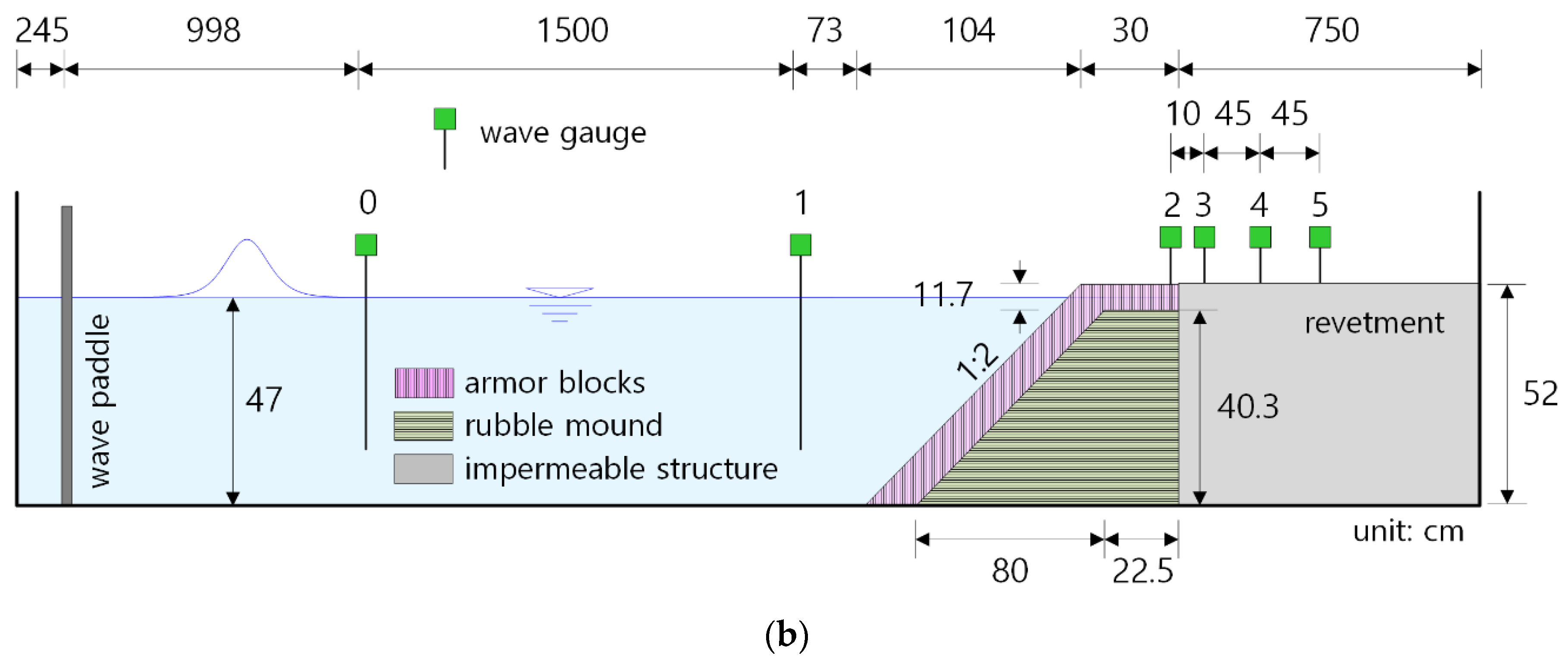
To investigate the characteristics of coastal inundation caused by solitary wave overtopping, we conducted a physical modeling test in a 2D wave flume, as shown in Figure 1a. A revetment was installed in a wave flume of 37 m length, 0.6 m width, and 1 m height. The sea area, including the wave maker, was 29.5 m, and the land area was 7.5 m. As shown in Figure 1a, a VR consisting of a vertical wall with a height of 52 cm was installed at a point 27.05 m away from the wave maker at a depth ($h$) of 47 cm in the wave flume. This impermeable revetment was made of waterproof plywood; the average roughness of the painted revetment surface was 0.56 mm (measured using 0918 Surface Roughness Tester from Hanchen). The WAR in Figure 1b consists of a rubble mound with a 1:2 slope, 0.46 porosity, and 2.2 g/ea average weight and is placed at the front of an impermeable vertical wall; the armor blocks on top form a double layer of tetrapods (TTPs) with 0.5 porosity and 368 g/ea average weight.

2.2. Free-Surface Tracking

In this experiment, the water surface elevation was measured at 50 Hz using six capacitance-type wave gauges (WGs). As shown in Figure 1, to set the incident wave and measure the reflected wave, WG0 was installed 998 cm away from the wave paddle, and WG1 was installed 207 cm away from the vertical wall. To measure the run-up height during solitary wave overtopping, WG2 was placed at a point 0.5 cm from the vertical wall. Further, in the experiment utilizing the WAR, a steel cage was installed to prevent interference between the armor blocks and rubble mound. To investigate the inundation process of solitary waves in the land area, WG3 to WG5 were installed 10 cm, 55 cm, and 100 cm away from the vertical wall toward the land, respectively. Owing to the nature of the capacitance-type WGs, it was not possible to measure water surface elevation changes of 0.5 cm or less in the land area.

2.3. Incident Wave Conditions

Table 1. Experimental conditions used in this study.

Run	$\mathit{h}$ (cm)	${\mathit{A}}_{\mathbf{0}} \mathbf{\left(}\mathbf{cm}\mathbf{\right)}$	${\mathit{L}}_{\mathit{e}} \mathbf{\left(}\mathbf{cm}\mathbf{\right)}$	$\mathit{\epsilon }$$\mathbf{(}{\mathit{A}}_{\mathbf{0}}\mathbf{/}\mathit{h}\mathbf{)}$	${\mathit{A}}_{\mathbf{0}}\mathbf{/}{\mathit{F}}_{\mathit{b}}$	${\mathit{A}}_{\mathbf{0}}\mathbf{/}{\mathit{L}}_{\mathit{e}}$
1	47	4.4	654.31	0.09	0.88	0.007
2		5.4	587.92	0.12	1.08	0.009
3		6.3	544.31	0.13	1.26	0.012
4		7.2	509.15	0.15	1.44	0.014
5		8.2	477.1	0.18	1.64	0.017
6		10	427.77	0.21	2	0.023
7		12.3	389.55	0.26	2.46	0.032
8		14.5	358.78	0.31	2.9	0.040
9		16.5	336.33	0.35	3.3	0.049
10		18.7	315.93	0.4	3.74	0.059
11		21.5	294.64	0.46	4.3	0.073

shows the incident conditions of the solitary waves applied in the physical modeling test. The incident wave height of the solitary wave ($A_0$) signifies the maximum water surface elevation (${\eta }_{max}$) at the time the waveform was measured by WG0. The 11 values of $A_0$ ranged from 4.4 to 21.5 cm. Accordingly, the relative wave height $\epsilon \left(A_0/h\right)$, which indicates the ratio of wave height to depth, varied from 0.09 to 0.46, and the ratio $A_0/F_b$ between the revetment crest height ($F_b)$ and $A_0$ varied from 0.88 to 4.3. The effective wavelength corresponding to 95% of the volume of the solitary wave waveform ($L_e$) was 294.64–654.31 cm, and the wave steepness ($A_0/L_e$) was 0.007–0.073. Here, $L_e$ can be obtained from the approximation theory of Dean and Dalrymple [34] as follows:

$$L_e=\frac{4.24h}{\sqrt{\epsilon }},$$

(1)

where $\epsilon$ is relative wave height ($=A_0/h$).

To create solitary waves from a piston-type wave maker with a stroke of ±0.55 m installed in the wave flume, the position signal ($X\left(t\right)$) of the wave paddle is needed. In this study, $X\left(t\right)$ was set [35] using Equation (2). To obtain the target wave height at WG0, a calibration process was conducted through repeated wave generation.

$$X\left(t\right)=\frac{2Ah \tanh \left(\frac{t}{2}\sqrt{\frac{3gA\left(A+h\right)}{h^2\left(A+h\right)}}\right)}{h\sqrt{\frac{3A}{h^2\left(A+h\right)}\left\{h+A\left[1-{\tanh }^2\left(\frac{t}{2}\sqrt{\frac{3gA\left(A+h\right)}{h^2\left(A+h\right)}}\right)\right]\right\}}},$$

(2)

where $A$ is the solitary wave amplitude and $g$ is the gravitational acceleration.

3. Experimental Results

3.1. Water Surface Elevation Distribution

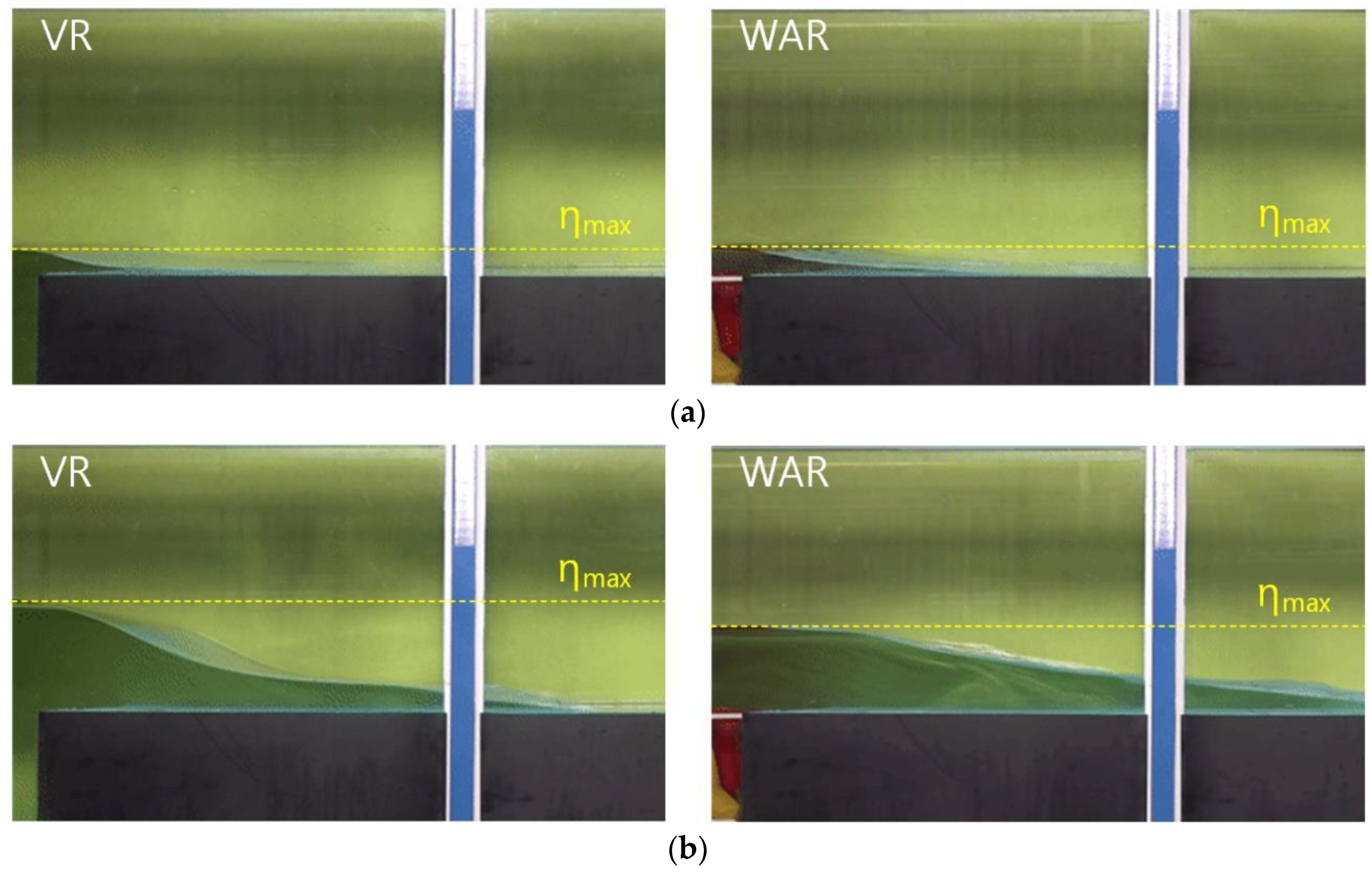
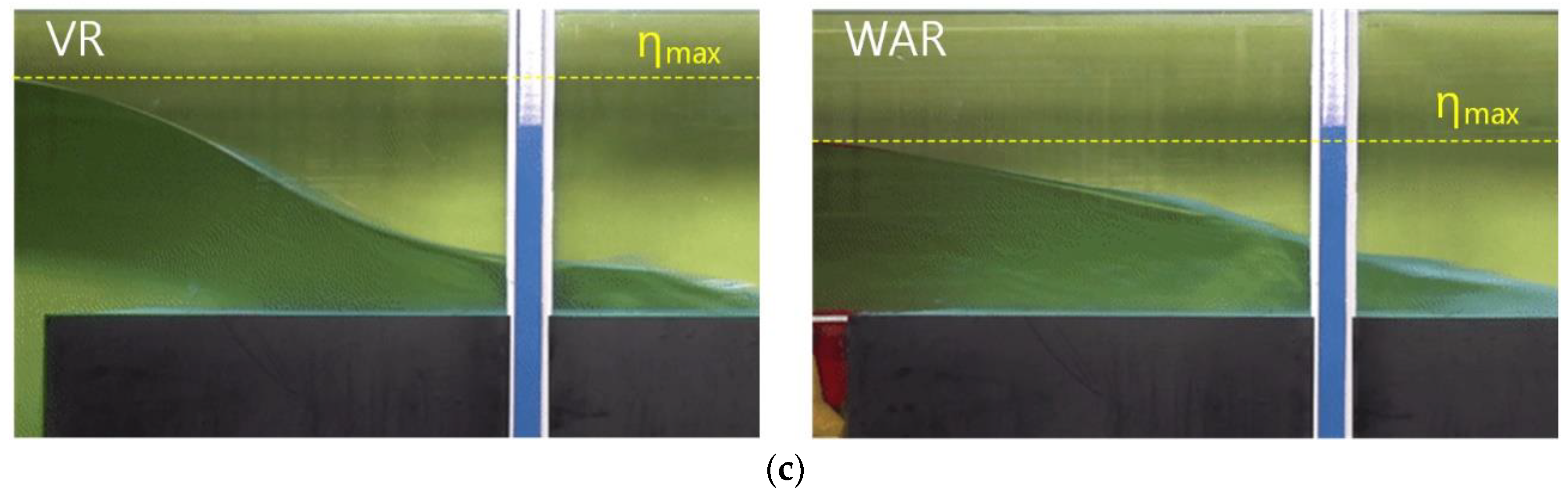
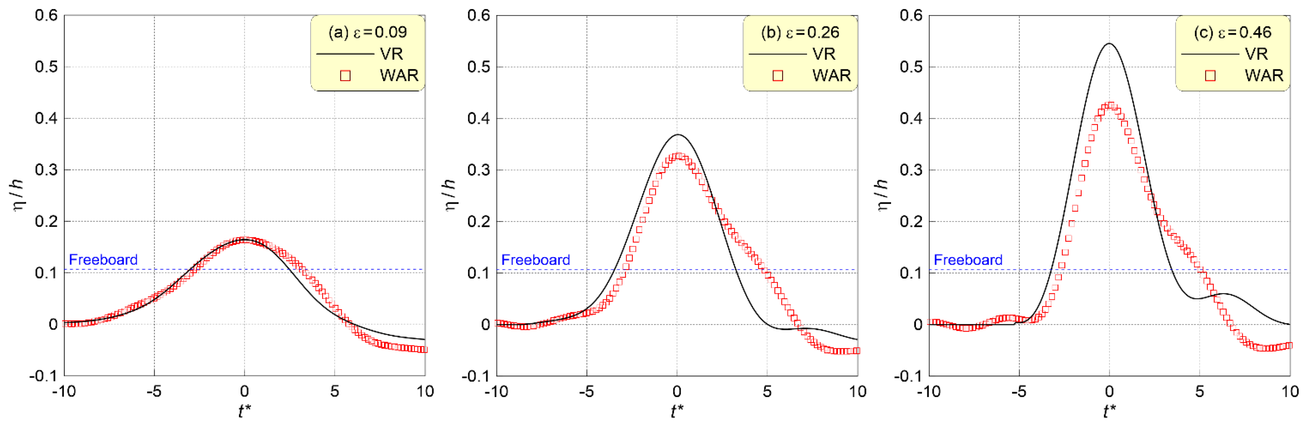
Figure 2 shows the overtopping and inundation of the solitary wave when the maximum water surface elevation (${\eta }_{max}$) occurs in front of the VR and WAR. Figure 3 shows the time waveforms measured at WG2 in front of the vertical wall in the overtopping and inundation process of the solitary wave. The maximum water surface elevation measured at WG2 during overtopping is shown in

Table A1. Maximum overtopping heights at the front of vertical wall (WG2).

Run	${\mathit{A}}_{\mathbf{0}} \mathbf{\left(}\mathbf{cm}\mathbf{\right)}$	$\mathit{\epsilon }$$\mathbf{(}{\mathit{A}}_{\mathbf{0}}\mathbf{/}\mathit{h}\mathbf{)}$	${\mathit{\eta }}_{\mathbf{m}\mathbf{a}\mathbf{x}}^{\mathbf{V}\mathbf{R}} \mathbf{\left(}\mathbf{cm}\mathbf{\right)}$	${\mathit{\eta }}_{\mathbf{m}\mathbf{a}\mathbf{x}}^{\mathbf{WAR}} \mathbf{\left(}\mathbf{cm}\mathbf{\right)}$	${\mathit{\eta }}_{\mathbf{m}\mathbf{a}\mathbf{x}}^{\mathbf{V}\mathbf{R}}\mathbf{/}\mathit{h}$	${\mathit{\eta }}_{\mathbf{m}\mathbf{a}\mathbf{x}}^{\mathbf{WAR}}\mathbf{/}\mathit{h}$	${\mathit{\eta }}_{\mathbf{m}\mathbf{a}\mathbf{x}}^{\mathbf{V}\mathbf{R}}\mathbf{/}{\mathit{A}}_{\mathbf{0}}$	${\mathit{\eta }}_{\mathbf{m}\mathbf{a}\mathbf{x}}^{\mathbf{WAR}}\mathbf{/}{\mathit{A}}_{\mathbf{0}}$	${\mathit{\eta }}_{\mathbf{m}\mathbf{a}\mathbf{x}}^{\mathbf{WAR}}\mathbf{/}{\mathit{\eta }}_{\mathbf{m}\mathbf{a}\mathbf{x}}^{\mathbf{V}\mathbf{R}}$
1	4.4	0.09	7.73	7.71	0.16	0.16	1.76	1.75	1.00
2	5.4	0.12	9.09	8.80	0.19	0.19	1.68	1.63	0.97
3	6.3	0.13	10.33	9.95	0.22	0.21	1.65	1.59	0.96
4	7.2	0.15	11.52	10.98	0.25	0.23	1.60	1.52	0.95
5	8.2	0.18	12.72	11.99	0.27	0.26	1.55	1.46	0.94
6	10	0.21	15.08	14.30	0.32	0.30	1.51	1.43	0.95
7	12.3	0.26	17.32	15.37	0.37	0.33	1.41	1.25	0.89
8	14.5	0.31	19.40	16.35	0.41	0.35	1.34	1.13	0.84
9	16.5	0.35	21.56	17.63	0.46	0.38	1.31	1.07	0.82
10	18.7	0.4	23.63	18.84	0.50	0.40	1.26	1.01	0.80
11	21.5	0.46	25.63	20.02	0.55	0.43	1.19	0.93	0.78

in the Appendix A.

The representative experimental conditions shown in Figure 2 and Figure 3 are Run-1 ($A_0=4.4 \mathrm{cm}$, $\epsilon =0.09$), Run-7 ($A_0=12.3 \mathrm{cm}$, $\epsilon =0.26$), and Run-11 ($A_0=21.5 \mathrm{cm}$, $\epsilon =0.46$). The vertical axis in Figure 3 is a dimensionless water surface elevation ($\eta /h$) calculated as the water surface displacement ($\eta$) divided by the water depth ($h$); its horizontal axis is the dimensionless time ($t^{*}=\left(t-t_2\right){\left(g/h\right)}^{1/2}$; $t_2$ is the time at which the maximum water surface elevation occurs at WG2).

Overtopping of the solitary waves was observed in Run-7 and Run-11 under the condition $A_0>F_b$, for which overtopping was expected to occur. As evidenced in Figure 2a and Figure 3a, overtopping occurs in both the VR and WAR even under the $A_0<F_b$ condition of Run-1. At the maximum water surface elevation during overtopping, the difference between the two maximum water surface elevations in Figure 2a, where $\epsilon$ is the smallest, is not large. However, as $\epsilon$ increases, the difference between the maximum water surface elevations at the VR and WAR increases. Lee et al. [33] analyzed the main cause of this trend through experiments and numerical analysis, which can be explained as follows.

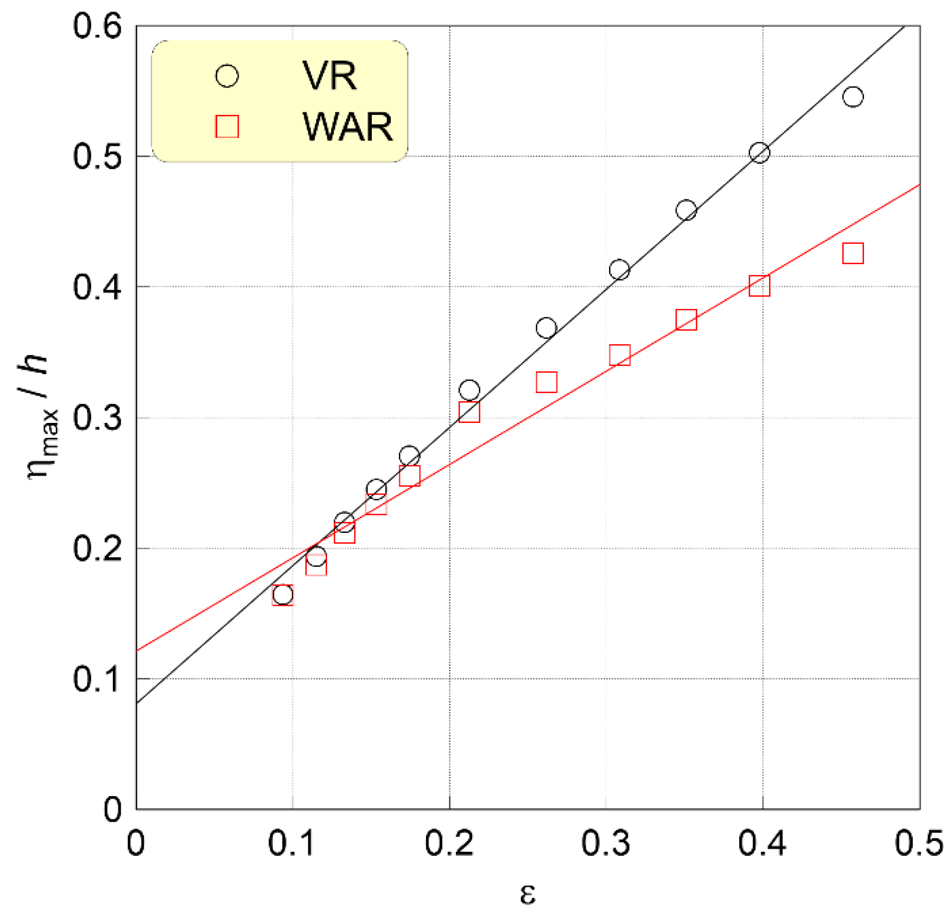
At the VR, because of a sharp decrease in the flow cross-sectional area, the horizontal velocity of the solitary wave is converted to vertical velocity, and overtopping occurs as the water surface elevation rises. Because the effective wavelength shortens as $\epsilon$ increases, the vertical velocity develops further, and the water surface elevation rises substantially during overtopping. Conversely, at the WAR, the flow cross-sectional area gradually decreases along the inclined wave absorber in front of the vertical wall. Thus, for the solitary wave passing through the inclined wave absorber, the horizontal and vertical velocities both develop along the slope, and the horizontal velocity becomes dominant above the crest. As a result, the rise in water surface elevation during solitary wave overtopping at the WAR does not exceed that at the VR; this trend is shown in Figure 4, which compares the dimensionless maximum water surface elevation (${\eta }_{\max }/h$) measured at WG2 in front of the vertical wall. Figure 4 shows a clear trend where ${\eta }_{\max }/h$ increases as $\epsilon$ increases, and the gradient is steeper at the VR than at the WAR. When $\epsilon$ is small, ${\eta }_{\max }/h$ at the VR and WAR does not show a difference, but the difference in ${\eta }_{\max }/h$ increases as $\epsilon$ increases.

Generally, for periodic waves, WAR has a smaller overtopping discharge than VR [36]. Baldock et al. [9] classified volume flux and freeboard as the factors significantly influencing wave overtopping. In a previous study by Lee et al. [33], the solitary wave showed a stronger flow property than the wave in the section with a small $\epsilon$. Thus, the wave overtopping discharge in WAR was higher than that in VR. The analysis of not only maximum water surface but also wave overtopping velocity is essential for the overtopping and flooding analysis, and the results related to this will be described in Section 5.

3.2. Water Surface Elevation Distribution in Land Area

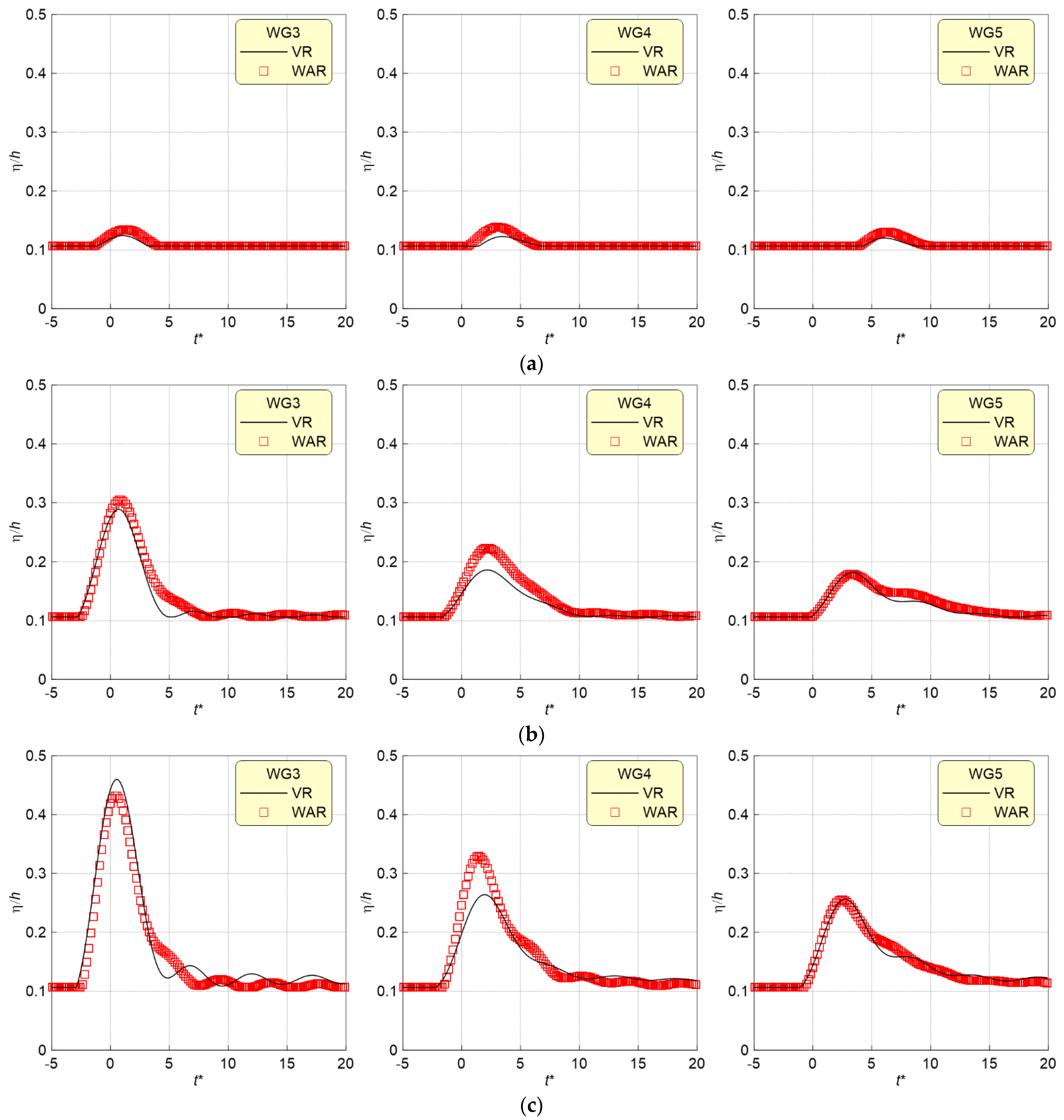
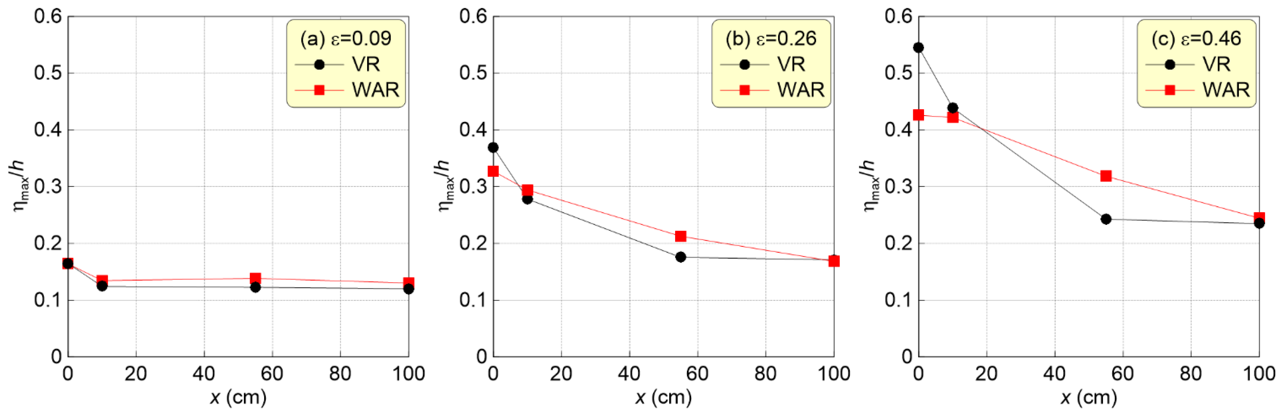
Figure 5 shows the time distribution of the water surface elevations measured at WG3, WG4, and WG5 installed in the land area when the solitary wave passes. Figure 6 shows the spatial distributions of the dimensionless maximum water surface elevations at WG2, WG3, WG4, and WG5. The representative experimental conditions of Run-1 ($A_0=4.4 \mathrm{cm}$, $\epsilon =0.09$), Run-7 ($A_0=12.3 \mathrm{cm}$, $\epsilon =0.26$), and Run-11 ($A_0=21.5 \mathrm{cm}$, $\epsilon =0.46$) are shown in (a), (b), and (c), respectively.

Figure 5 and Figure 6 show the phenomena where during solitary wave overtopping, the maximum water surface elevation decreases with increasing distance from the revetment, and this trend intensifies with an increase in $\epsilon$. In Figure 4, the maximum water surface elevation measured at WG2 in front of the vertical wall is high at the VR, although the maximum water surface elevation of WG3 located 10 cm from the revetment in Figure 5 does not show a large difference. In addition, the maximum water surface elevation for the WAR at WG4, 55 cm from the revetment, was measured to be higher than that at the VR. At WG5, 100 cm away from the revetment, the difference in the maximum water surface elevation between the VR and WAR decreased. As depicted in Figure 6, during overtopping at WG2 ($x=0 \mathrm{cm}$) in front of the revetment, ${\eta }_{\max }/h$ increased as $\epsilon$ increased, but at WG3 ($x=10 \mathrm{cm}$), the difference in ${\eta }_{\max }/h$ was not large. Additionally, at WG4 ($x=55 \mathrm{cm}$), ${\eta }_{\max }/h$ at the WAR was larger than that at the VR, and at WG5 ($x=100 \mathrm{cm}$), ${\eta }_{\max }/h$ again became similar for the VR and WAR. The previous study by Lee et al. [33] showed no difference in wave overtopping with revetment type. Thus, the maximum water surface elevation during overtopping differed marginally with the revetment type at the front; however, the difference did not increase as the wave propagated to the land area. As mentioned, because vertical velocity was dominant in VR when overtopping, maximum water surface elevation (WG3) was higher. In WAR, horizontal flow velocity was dominant to proceed with the inundation; thus, the decrease in maximum water surface elevation was smaller than in VR. In practice, the superposition of incident and reflected waves increases the maximum water surface elevation of WG3, and it is relatively low in WAR due to energy loss in front of the structure because the reflection is lower in WAR than in VR [32].

3.3. Maximum Inundation Height

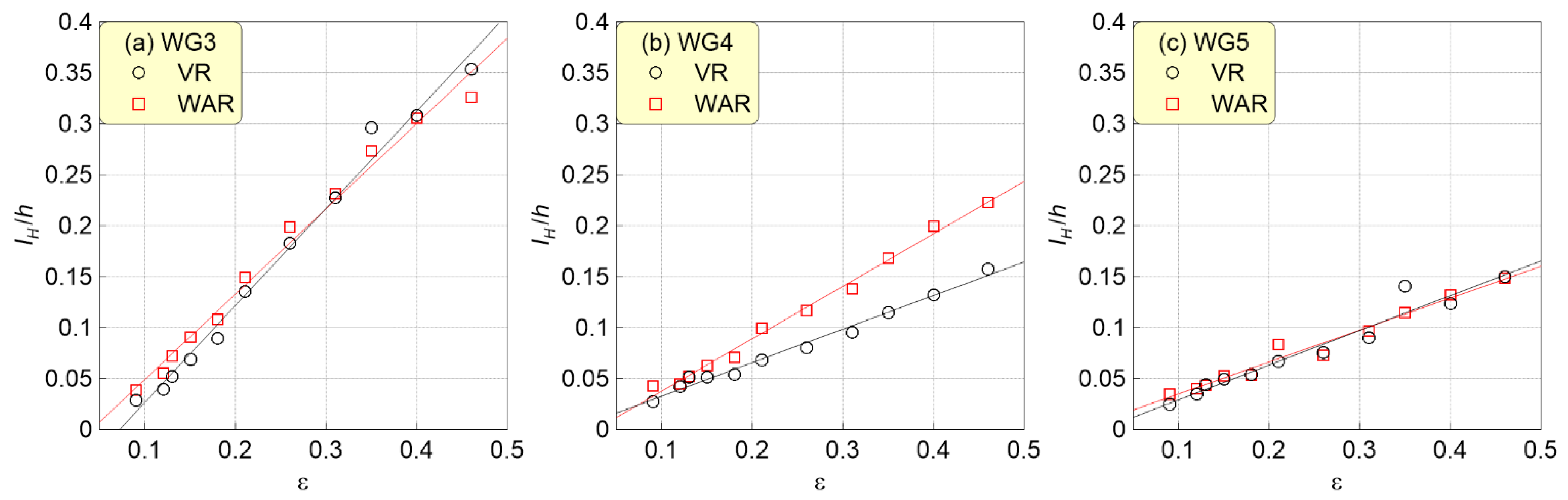
The maximum inundation height ($I_H$) is based on the surface of the land area; the freeboard ($F_b$) of the revetment is subtracted from the maximum water surface elevation (${\eta }_{max}$) of the solitary wave and then nondimensionalized through $h$; the results are shown in Figure 7. The maximum inundation heights measured at WG3, WG4, and WG5 through the physical modeling test are recorded in

Table A2. Maximum inundation heights at WG3 ($x/h=0.21$).

Run	${\mathit{A}}_{\mathbf{0}} \mathbf{\left(}\mathbf{cm}\mathbf{\right)}$	$\mathit{\epsilon }$$\mathbf{(}{\mathit{A}}_{\mathbf{0}}\mathbf{/}\mathit{h}\mathbf{)}$	${\mathit{D}}_{\mathit{H}}^{\mathbf{V}\mathbf{R}} \mathbf{\left(}\mathbf{cm}\mathbf{\right)}$	${\mathit{D}}_{\mathit{H}}^{\mathbf{WAR}} \mathbf{\left(}\mathbf{cm}\mathbf{\right)}$	${\mathit{D}}_{\mathit{H}}^{\mathbf{V}\mathbf{R}}\mathbf{/}\mathit{h}$	${\mathit{D}}_{\mathit{H}}^{\mathbf{WAR}}\mathbf{/}\mathit{h}$	${\mathit{D}}_{\mathit{H}}^{\mathbf{V}\mathbf{R}}\mathbf{/}{\mathit{A}}_{\mathbf{0}}$	${\mathit{D}}_{\mathit{H}}^{\mathbf{WAR}}\mathbf{/}{\mathit{A}}_{\mathbf{0}}$	${\mathit{D}}_{\mathit{H}}^{\mathbf{WAR}}\mathbf{/}{\mathit{D}}_{\mathit{H}}^{\mathbf{V}\mathbf{R}}$
1	4.4	0.09	1.34	1.82	0.03	0.04	0.31	0.41	1.36
2	5.4	0.12	1.85	2.58	0.04	0.05	0.34	0.48	1.39
3	6.3	0.13	2.43	3.37	0.05	0.07	0.39	0.54	1.38
4	7.2	0.15	3.21	4.25	0.07	0.09	0.45	0.59	1.32
5	8.2	0.18	4.18	5.07	0.09	0.11	0.51	0.62	1.21
6	10	0.21	6.35	7.03	0.14	0.15	0.64	0.70	1.11
7	12.3	0.26	8.57	9.33	0.18	0.20	0.70	0.76	1.09
8	14.5	0.31	10.67	10.88	0.23	0.23	0.74	0.75	1.02
9	16.5	0.35	13.91	12.85	0.30	0.27	0.84	0.78	0.92
10	18.7	0.4	14.48	14.34	0.31	0.31	0.77	0.77	0.99
11	21.5	0.46	16.61	15.33	0.35	0.33	0.77	0.71	0.92

,

Table A3. Maximum inundation heights at WG4 ($x/h=1.17$).

Run	${\mathit{A}}_{\mathbf{0}} \mathbf{\left(}\mathbf{cm}\mathbf{\right)}$	$\mathit{\epsilon }$$\mathbf{(}{\mathit{A}}_{\mathbf{0}}\mathbf{/}\mathit{h}\mathbf{)}$	${\mathit{D}}_{\mathit{H}}^{\mathbf{V}\mathbf{R}} \mathbf{\left(}\mathbf{cm}\mathbf{\right)}$	${\mathit{D}}_{\mathit{H}}^{\mathbf{WAR}} \mathbf{\left(}\mathbf{cm}\mathbf{\right)}$	${\mathit{D}}_{\mathit{H}}^{\mathbf{V}\mathbf{R}}\mathbf{/}\mathit{h}$	${\mathit{D}}_{\mathit{H}}^{\mathbf{WAR}}\mathbf{/}\mathit{h}$	${\mathit{D}}_{\mathit{H}}^{\mathbf{V}\mathbf{R}}\mathbf{/}{\mathit{A}}_{\mathbf{0}}$	${\mathit{D}}_{\mathit{H}}^{\mathbf{WAR}}\mathbf{/}{\mathit{A}}_{\mathbf{0}}$	${\mathit{D}}_{\mathit{H}}^{\mathbf{WAR}}\mathbf{/}{\mathit{D}}_{\mathit{H}}^{\mathbf{V}\mathbf{R}}$
1	4.4	0.09	1.27	2.01	0.03	0.04	0.29	0.46	1.59
2	5.4	0.12	1.97	2.10	0.04	0.04	0.36	0.39	1.07
3	6.3	0.13	2.42	2.44	0.05	0.05	0.39	0.39	1.01
4	7.2	0.15	2.41	2.95	0.05	0.06	0.34	0.41	1.22
5	8.2	0.18	2.55	3.31	0.05	0.07	0.31	0.40	1.30
6	10	0.21	3.20	4.67	0.07	0.10	0.32	0.47	1.46
7	12.3	0.26	3.75	5.49	0.08	0.12	0.30	0.45	1.47
8	14.5	0.31	4.47	6.49	0.10	0.14	0.31	0.45	1.45
9	16.5	0.35	5.38	7.89	0.11	0.17	0.33	0.48	1.47
10	18.7	0.4	6.21	9.37	0.13	0.20	0.33	0.50	1.51
11	21.5	0.46	7.41	10.46	0.16	0.22	0.34	0.49	1.41

and

Table A4. Maximum inundation heights at WG5 ($x/h=2.13$).

Run	${\mathit{A}}_{\mathbf{0}} \mathbf{\left(}\mathbf{cm}\mathbf{\right)}$	$\mathit{\epsilon }$$\mathbf{(}{\mathit{A}}_{\mathbf{0}}\mathbf{/}\mathit{h}\mathbf{)}$	${\mathit{D}}_{\mathit{H}}^{\mathbf{V}\mathbf{R}} \mathbf{\left(}\mathbf{cm}\mathbf{\right)}$	${\mathit{D}}_{\mathit{H}}^{\mathbf{WAR}} \mathbf{\left(}\mathbf{cm}\mathbf{\right)}$	${\mathit{D}}_{\mathit{H}}^{\mathbf{V}\mathbf{R}}\mathbf{/}\mathit{h}$	${\mathit{D}}_{\mathit{H}}^{\mathbf{WAR}}\mathbf{/}\mathit{h}$	${\mathit{D}}_{\mathit{H}}^{\mathbf{V}\mathbf{R}}\mathbf{/}{\mathit{A}}_{\mathbf{0}}$	${\mathit{D}}_{\mathit{H}}^{\mathbf{WAR}}\mathbf{/}{\mathit{A}}_{\mathbf{0}}$	${\mathit{D}}_{\mathit{H}}^{\mathbf{WAR}}\mathbf{/}{\mathit{D}}_{\mathit{H}}^{\mathbf{V}\mathbf{R}}$
1	4.4	0.09	1.15	1.62	0.02	0.03	0.26	0.37	1.42
2	5.4	0.12	1.62	1.89	0.03	0.04	0.30	0.35	1.17
3	6.3	0.13	2.06	2.03	0.04	0.04	0.33	0.32	0.98
4	7.2	0.15	2.32	2.46	0.05	0.05	0.32	0.34	1.06
5	8.2	0.18	2.52	2.51	0.05	0.05	0.31	0.31	1.00
6	10	0.21	3.11	3.92	0.07	0.08	0.31	0.39	1.26
7	12.3	0.26	3.55	3.41	0.08	0.07	0.29	0.28	0.96
8	14.5	0.31	4.23	4.55	0.09	0.10	0.29	0.31	1.07
9	16.5	0.35	6.62	5.39	0.14	0.11	0.40	0.33	0.82
10	18.7	0.4	5.79	6.21	0.12	0.13	0.31	0.33	1.07
11	21.5	0.46	7.04	6.99	0.15	0.15	0.33	0.33	0.99

in the Appendix A.

Figure 7 shows an increasing trend of the dimensionless maximum inundation height ($I_H/h$) with an increase in $\epsilon$. At WG4 in (b), characteristics contrary to those of the maximum water surface elevation at the front of the revetment in Figure 4 are observed. In other words, at WG4, which is $x/h=1.17$ from the shoreline, where the water surface gradient is steep, as shown in Figure 2, $I_H/h$ is greater at the VR than at the WAR, and as $\epsilon$ increases, the water surface gradient steepens, thus increasing the difference. Moreover, at WG5 ($x/h=2.13$) in (c), $I_H/h$ does not differ greatly between VR and WAR, and there is no clear trend. At WG3 ($x/h=0.21$) in (a), $I_H/h$ is larger at the WAR when $\epsilon <0.3$ and larger at the VR when $\epsilon >0.3$.

Hence, it is difficult to analyze the inundation characteristics at the VR and WAR based on only the water surface elevation data of solitary waves obtained through physical modeling tests. Accordingly, this study investigated the inundation process of solitary waves by simulating the wave fields and flow fields using an NWT.

4. Numerical Methodology

4.1. Numerical Model

This study conducted a numerical analysis to examine the infiltration characteristics of solitary waves at the VR and WAR and analyze the effect on overtopping and inundation of the wave absorber in front of the revetment. The NWT [33] used for numerical analysis was improved by implementing a dynamic eddy viscosity model [37,38] and continuum surface force model [39] using the N–S equation model modified based on the porous body model (PBM) and LES [40]. In addition, Lee et al. [33] proposed a wave generation method for solitary waves to simulate solitary wave overtopping in the NWT. Details of the numerical analysis technique of the numerical model used in this study are available in the previous reports by Lee et al. [33,41].

4.1.1. Governing Equations

In LES, the spatially filtered continuity and modified N–S momentum equations, including the PBM for a viscous and incompressible fluid with constant density, are given as:

$$\frac{\partial \left({\gamma }_i{v}_i\right)}{\partial x_i}=q^{*},$$

(3)

$${\gamma }_v\frac{\partial v_i}{\partial t}+\frac{\partial \left(v_i{\gamma }_j{v}_j\right)}{\partial x_j}=-\frac{{\gamma }_v}{\rho }\frac{\partial p}{\partial x_i}+\frac{\partial }{\partial x_j}{\gamma }_j{\nu }_T\left(\frac{\partial v_i}{\partial x_j}+\frac{\partial v_j}{\partial x_i}\right)+S_i-Q_i-R_i-G_i-E_i,$$

(4)

where $v_i$ represents the horizontal and vertical velocity components; $x_i$ is the Cartesian coordinate system, with the $x$-axis as the direction of wave propagation and $z$-axis pointing vertically upward; $t$ denotes the time; ${\gamma }_v$ and ${\gamma }_i$ are the volume and surface porosities, respectively; $\rho$ is the fluid density; $p$ is the fluid pressure; ${\nu }_T$ is the sum of the kinematic viscosity coefficient ($\nu$) and eddy viscosity coefficient (${\nu }_t$); $S_i$ is the surface tension force; $R_i$ is the fluid resistance term for a porous media; $G_i$ is the gravitational acceleration term ($={\gamma }_{v}g$); $E_i$ is the wave energy damping term ($=-\beta w$, where $\beta$ is the damping factor equal to $0$, except for the added damping zones) for the vertical velocity only; $Q_i$ refers to the wave source terms ($=\frac{2\nu }{3}\frac{\partial q^{*}}{\partial x_i}$); $q^{*}$ is the flux density according to the grid sizes required to generate waves only at the source position $x=x_s$, defined as:

$$q^{*}=\{\begin{array}{cc}q\left(z,t\right)/\mathsf{\Delta }{x}_s& x=x_s\\ 0& x\ne x_s\end{array},$$

(5)

where $q$ is the raw flux density; and $\mathsf{\Delta }{x}_s$ is the horizontal grid size at the source position ($x_s$).

A numerical simulation of the fluid flow on a free surface requires not only solutions of the governing equations (continuity and momentum equations) but also the special treatment of the free surface (i.e., tracking of the fluid interface). $F$ denotes the volume of fluid (VOF) in each cell [42], which can be expressed in terms of fluid conservation by applying an assumption of fluid incompressibility and a function volume based on the PBM, as follows:

$${\gamma }_v\frac{\partial F}{\partial t}+\frac{\partial \left({\gamma }_i{v}_{i}F\right)}{\partial x_i}=Fq \ast ,$$

(6)

where $F$ is the VOF function. In the numerical simulation, each cell was assigned as one of the following three types based on the VOF function value: fluid cell ($F=1$), empty cell ($F=0$), and free-surface cell ($0<F<1$).

4.1.2. Solution Techniques

A staggered grid is used for computational discretization, where the velocity components are stored at the cell face, and other variables, including the pressure, wave source function, and VOF function, are defined at the cell center. The governing equations are converted to a system of algebraic equations using the finite difference method (FDM). For the discretization of the N–S momentum equation (Equation (4)), we use the forward difference approximation for the time derivative terms, the combination of the central difference method and upwind method for the convection term, and the central difference approximation for the other terms including the pressure gradient and stress. The finite difference approximations of Equation (4) can be written as follows:

$$v_i^{n+1}=v_i^n+\frac{\mathsf{\Delta }t}{{\gamma }_v}\left\{\left(A_i+V_i+S_i+O_i\right)-\frac{1}{\rho }\frac{p_{i+1}^{n+1}-p_i^{n+1}}{\frac{1}{2}\left(\mathsf{\Delta }{x}_{i+1}+\mathsf{\Delta }{x}_i\right)}\right\},$$

(7)

where $A_i$ represents the advection term; $V_i$ is the viscosity term; $S_i$ is the source term; $O_i$ denotes the additional terms in Equation (4); and $\mathsf{\Delta }t$ is the time increment.

From the discretized Equation (7), the new water particle velocity $v_i^{n+1}$ can be calculated explicitly using the initial conditions or velocities and the pressure at the previous time level $n$. However, the new velocities obtained using the above momentum equations do not generally satisfy the continuity equation (Equation (3)) in a control volume (cell), i.e., the pressure in each cell has to be controlled for the velocity to satisfy the continuity equation. Hence, an iterative calculation is required for the pressure at each cell. We adopted the SOLA scheme, also called the highly simplified marker and cell technique, proposed by Hirt and Nichols [42], to compute the correction component for the pressure at each cell, $\Delta p$. The SOLA scheme is conceptually simple and easy to implement because it uses an iterative successive over-relaxation method instead of a matrix solver.

By using the correction component for pressure, all water particle velocities at each cell are updated as follows:

$${}_{}{}^{m+1}v^{n+1}={}_{}{}^{m}v^n+\frac{1}{\rho }\frac{\mathsf{\Delta }t}{\mathsf{\Delta }{x}_i}\left({}^m\Delta p^{n+1}\right),$$

(8)

where the superscript $m$ denotes the number of iterations at each time step. After the velocity components and pressure have been calculated, the new free-surface configuration is computed using the advection equation of the VOF function (Equation (6)), which is solved by using the donor–acceptor method [42].

4.1.3. Fluid Resistance

Based on the modified N–S momentum equation (Equation (4)), the fluid resistance for a flow through a porous media $R_i$ is expressed as:

$$R_i=\left[C_L\frac{\nu {\left(1-{\gamma }_i\right)}^2}{{\gamma }_i^3{d}_{50}^2}+C_T\frac{\left(1-{\gamma }_i\right)}{{\gamma }_i^3{d}_{50}}\sqrt{{\left({\gamma }_i{v}_i\right)}^2+{\left({\gamma }_j{v}_j\right)}^2}\right]{\gamma }_i{v}_i+C_I\left(1-{\gamma }_i\right)\frac{\partial \left({\gamma }_i{v}_i\right)}{\partial t},$$

(9)

where $C_L$ is the coefficient of laminar resistance; $C_T$ is the coefficient of turbulent resistance; $C_M$ is the coefficient of inertia; and $d_{50}$ is the median grain size of the porous media.

The fluid resistances include the frictional resistance forces due to laminar flow (viscous effect) [43], frictional resistance forces due to turbulent flow (turbulence effect) [44], and inertial resistance force suggested in [45].

4.1.4. Turbulence Model

To determine the eddy viscosity (${\nu }_t$), the simple Smagorinsky subgrid-scale model [46] is adopted as follows:

$${\nu }_t={\left(C_s\mathsf{\Delta }\right)}^2{\left\{2{\left(\frac{\partial v_i}{\partial x_i}\right)}^2+2{\left(\frac{\partial v_j}{\partial x_j}\right)}^2+{\left(\frac{\partial v_i}{\partial x_j}+\frac{\partial v_j}{\partial x_i}\right)}^2\right\}}^{1/2},$$

(10)

where $C_s$ is the Smagorinsky’s constant; and $\Delta$ is the filter length-scale considered as the square root of the computational grid area.

In the eddy viscosity model, $C_s$ should be applied differently depending on the flow characteristics; however, a fixed value is often used in numerical models with LES [40,47]. The appropriate $C_s$ can be calculated through the dynamic modeling procedure suggested by Germano et al. [37] and Lilly [38]. The dynamic modeling procedure expresses the physical quantity included in the analytical grid as functions of time and space. This procedure does not require prior designation of unknown $C_s$ or fine-tuning and can accurately predict laminar flow and asymptotic behavior near walls.

4.1.5. Boundary Conditions

Two free-surface boundary conditions (i.e., normal and tangential stress conditions) were used to create the time-marching scheme of free-surface motion. The normal stress condition was imposed as a boundary condition for pressure. The pressure point defined at the center of a cell generally differs from the actual location on the free surface. Therefore, the pressure at the center of the surface cell was evaluated using linear interpolation or extrapolation between the pressure on the free surface and that on the adjacent fluid cell. The tangential boundary condition was imposed by assuming the same velocities outside the fluid domain as those inside (zero gradient boundary condition on the free surface). Furthermore, the velocities at the interfaces between the surface and empty cells were determined such that the continuity equation was satisfied.

The impermeable and non-slip conditions were applied to the normal and tangential directions with respect to the bottom and surface of the impermeable structure, respectively. In addition, at the offshore boundary of the NWT, the radiation condition (open boundary) in which the change in a physical quantity ($\varphi$), such as the velocity or VOF function, becomes $0$, was expressed as follows:

$$\frac{\partial \varphi }{\partial t}\pm \frac{\partial \varphi }{\partial x_i}=0.$$

(11)

An NWT using the FDM undergoes a discretization process based on a rectangular grid system. In this procedure, because the sloped or circular structure must be processed in stages, distortion occurs in the surface grid of the structure. To mitigate this problem, Lee et al. [48] proposed a reasonable boundary based on the method of Petit et al. [49] for creating a circular pipe through polygons. Lee et al. [13] investigated an impermeable sloped beach by applying a reasonable boundary to a 3D NWT. Hur et al. [50] and Lee et al. [41] extended this further to investigate not only impermeable sloped structures but also permeable sloped surfaces in a 3D NWT. This study processed the sloped surface of the permeable wave absorber of WAR using a reasonable boundary.

4.1.6. Stability Conditions

In computational fluid dynamics, the stability of the calculation, which is related to the convergence of the numerical solution, is critical. To ensure the stability of the calculation, the Courant–Friedrichs–Lewy (CFL) condition and diffusive limit (DL) condition were imposed to determine the $\mathsf{\Delta }t$. The CFL and DL conditions can be expressed as follows:

$$\mathsf{\Delta }t<\mathsf{\kappa }\cdot \min \left(\frac{\mathsf{\Delta }{x}_i}{{\left|v_i\right|}_{\max }}, \frac{\mathsf{\Delta }{x}_j}{{\left|v_j\right|}_{\max }}\right),$$

(12)

$$\mathsf{\Delta }t<\frac{1}{2}{\left[v\left(\frac{1}{\mathsf{\Delta }{x}_i^2+\mathsf{\Delta }{x}_j^2}\right)\right]}^{-1},$$

(13)

where $\mathsf{\Delta }{x}_i$ and ${\left|v_i\right|}_{\max }$ are the grid size and maximum velocity in the $x_i$ direction; $\mathsf{\kappa }$ is the weight coefficient, which is set as $\mathsf{\kappa }=0.5$ in most cases; and $\mathsf{\Delta }t=1/1000 \mathrm{s}$ is used as the initial time increment, after which $\mathsf{\Delta }t$ is adjusted automatically at the time of each calculation to satisfy the CFL and DL conditions.

4.2. NWT Setup

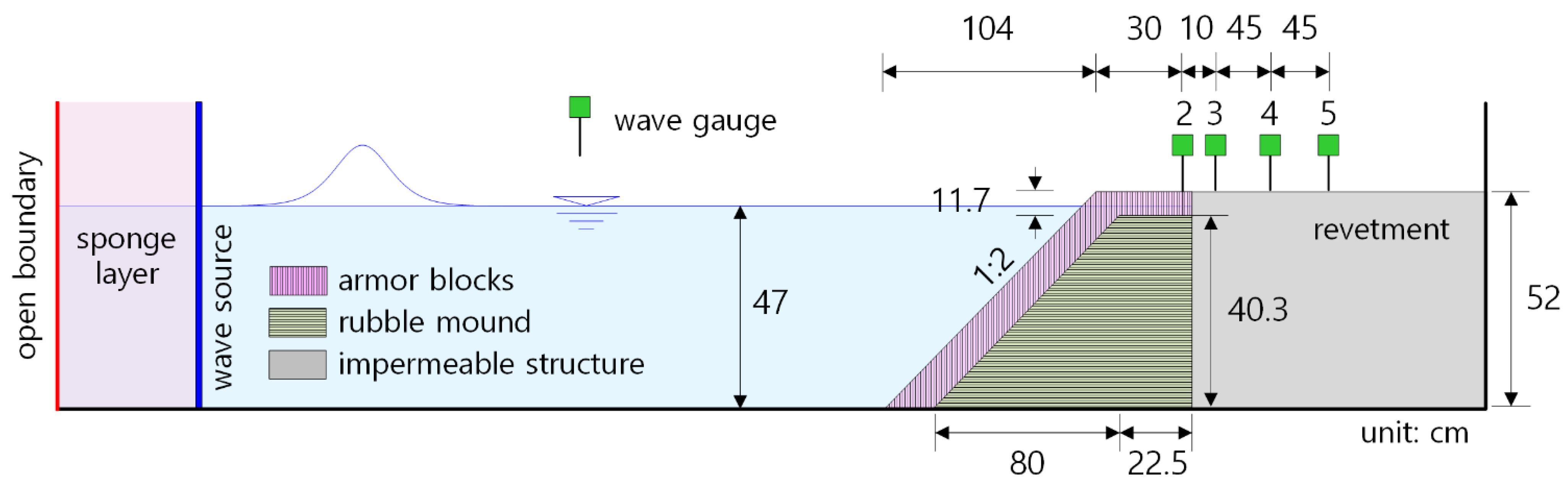
In this numerical analysis, an NWT was constructed with the same specifications as the experimental tank, as shown in Figure 8. We applied the same specifications for the VR and WAR in the NWT as used in the experiment. For the WAR, the volumetric porosity (${\gamma }_v$) and average particle diameter ($d_{50}$) of the rubble mound were 0.46 and 1.62 cm, respectively; ${\gamma }_v$ of the wave absorbing blocks, which were TTPs, was 0.5; and the characteristic length ($l_c$) of 5.43 cm obtained from Equation (14) was applied to $d_{50}$. In the NWT, a wave-generating source was installed at the same position as the wave maker in the experimental tank, and a sponge layer and an open boundary were placed in the open sea.

$$l_c={\left(\frac{W}{{\gamma }_s}\right)}^{1/3},$$

(14)

where $W$ is the weight of the TTP blocks, and ${\gamma }_s$ is the unit weight of plain concrete.

4.3. Wave Generation and Verification

4.3.1. Wave Generation Conditions

The non-reflected wave generation system proposed by Brorsen and Larsen [51] has twice the generation intensity because waves propagate in both directions ($\pm x$ directions). When long-period waves, such as solitary waves, are generated in an NWT of limited length, the target waveform cannot be accurately generated because reflected waves can be introduced as wave sources during wave generation. For the stable generation of solitary waves in an NWT, the wave generation intensity ($\zeta$) of Ohyama and Nadaoka [52], which can remove the influence of the reflected waves, was introduced as follows:

$$q\left(z,t\right)=2U_i\zeta ,$$

(15)

where $U_i$ is the horizontal velocity based on the wave theory; $\zeta$ is the intensity factor ($=\frac{{\eta }_i+h}{{\eta }_s+h}$; ${\eta }_s$ is the water surface elevation at the source position; and ${\eta }_i$ is the theoretical water surface elevation). The constant “$2$” accounts for the two waves propagating to the left and right sides in the NWT.

In this study, eleven different solitary waves were generated at the wave source in the NWT, with the specified water surface elevation and velocity based on an approximation theory [34]. The following formulae for the water surface elevation and horizontal velocity are substituted into the expression for the flux density of the wave source:

$${\eta }_i\left(x,t\right)=A_0{\mathrm{sech}}^2\left[\sqrt{\frac{3A_0}{4h^3}}\left(x-Ct\right)\right],$$

(16)

$$U_i\left(x,z,t\right)=\frac{\eta }{A_0}\left\{\epsilon +3{\epsilon }^2\left[\frac{1}{6}-\frac{1}{2}{\left(\frac{z}{h}\right)}^2\right]\right\}-{\left(\frac{\eta }{A_0}\right)}^2\left\{{\epsilon }^2\left[\frac{7}{4}-\frac{9}{4}{\left(\frac{z}{h}\right)}^2\right]\right\},l_c={\left(\frac{W}{{\gamma }_s}\right)}^{1/3},$$

(17)

$$W_i\left( x,z, t\right)=C\sqrt{3\epsilon }\frac{z}{h}\frac{\eta }{A_0}\tanh \left[k\left(x-Ct\right)\right]\left\{1+\frac{1}{2}\epsilon \left[1-7\frac{\eta }{A_0}-{\left(\frac{z}{h}\right)}^2\left(1-3\frac{\eta }{A_0}\right)\right]\right\},$$

(18)

where ${\eta }_i\left(x,t\right)$ is the solitary waveform based on the Boussinesq assumption; $\sqrt{\frac{3A_0}{4h^3}}$ is the effective wavenumber; and $C$ is the wave celerity ($=\sqrt{gh}\left(1+\frac{A_0}{2h}\right)$).

4.3.2. Grid Resolution Test

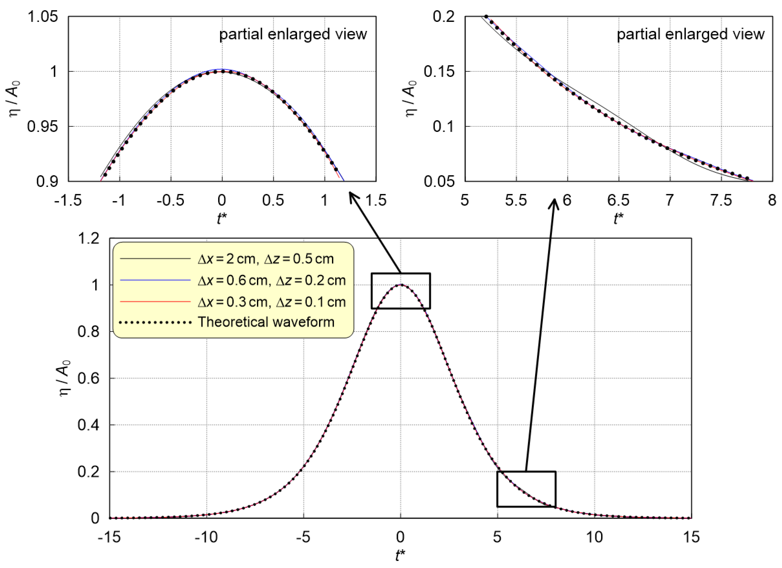
To verify the accuracy of the numerical analysis according to the grid resolution used for the NWT, solitary waves were generated by considering three grid sizes. We conducted a grid resolution test for the Run-1 condition in Table 1 ($A_0=4.4 \mathrm{cm}$, $\epsilon =0.09$), which is the smallest wave height. The three grid resolutions were tested by applying the maximum (Test-1), minimum (Test-2), and half (Test-3) grid sizes applied for the NWT, which are shown in

Table 2. Grid sizes used for resolution test.

Test	$\mathbf{\Delta }\mathit{x} \mathbf{\left(}\mathbf{cm}\mathbf{\right)}$	$\mathbf{\Delta }\mathit{z} \mathbf{\left(}\mathbf{cm}\mathbf{\right)}$	${\mathit{L}}_{\mathit{e}}\mathbf{/}\mathbf{\Delta }\mathit{x}$	${\mathit{A}}_{\mathbf{0}}/\mathbf{\Delta }\mathit{z}$	$\mathbf{\Delta }\mathit{z}\mathbf{/}\mathbf{\Delta }\mathit{x}$
1	2	0.5	327.2	8.8	1/4
2	0.6	0.2	3271.6	22.0	1/3
3	0.3	0.1	6543.1	44.0	1/3

.

Figure 9 shows the incident waveforms of the solitary waves generated with each of the three grid resolutions applied for the NWT. For all grid resolution conditions, the approximate waveforms reported by Dean and Dalrymple [34] were reproduced very accurately. First, at the wave crest sections, Test-3 ($\Delta x=0.3 \mathrm{cm}$, $\Delta x=0.1 \mathrm{cm}$), which had the finest grid resolution, showed the greatest consistency with the theoretical waveform, whereas Test-1 ($\Delta x=2 \mathrm{cm}$, $\Delta x=0.5 \mathrm{cm}$), which had a relatively coarse grid resolution, slightly overestimated the waveform distribution, and Test-2 ($\Delta x=0.6 \mathrm{cm}$, $\Delta x=0.2 \mathrm{cm}$) slightly overestimated the wave height. In the waveform distribution where the water surface elevation of the solitary wave was decreasing, there was slight oscillation for the coarse resolution of Test-1, whereas the results of Test-2 and Test-3 were nearly identical to the theoretical waveform.

Because the numerical error reduces as the precision of the grid resolution increases, solitary waves close to the theoretical waveform can be generated in the NWT. However, indiscriminately increasing the NWT grid resolution can cause the computational load to become excessively large. Accordingly, after comprehensively evaluating the grid resolution test results, we divided the analysis area of the NWT into a grid with 2 cm intervals horizontally and 0.5 cm intervals vertically. In addition, near the structures and still water surface elevation where the fluid motion was active, horizontal and vertical grid sizes of 0.6 cm and 0.2 cm were used to minimize the free-surface distortion and numerical diffusion. In addition, we gradually downscaled the grid by placing a relaxation layer in the transition from coarse grid resolution to medium grid resolution.

4.3.3. NWT Verification

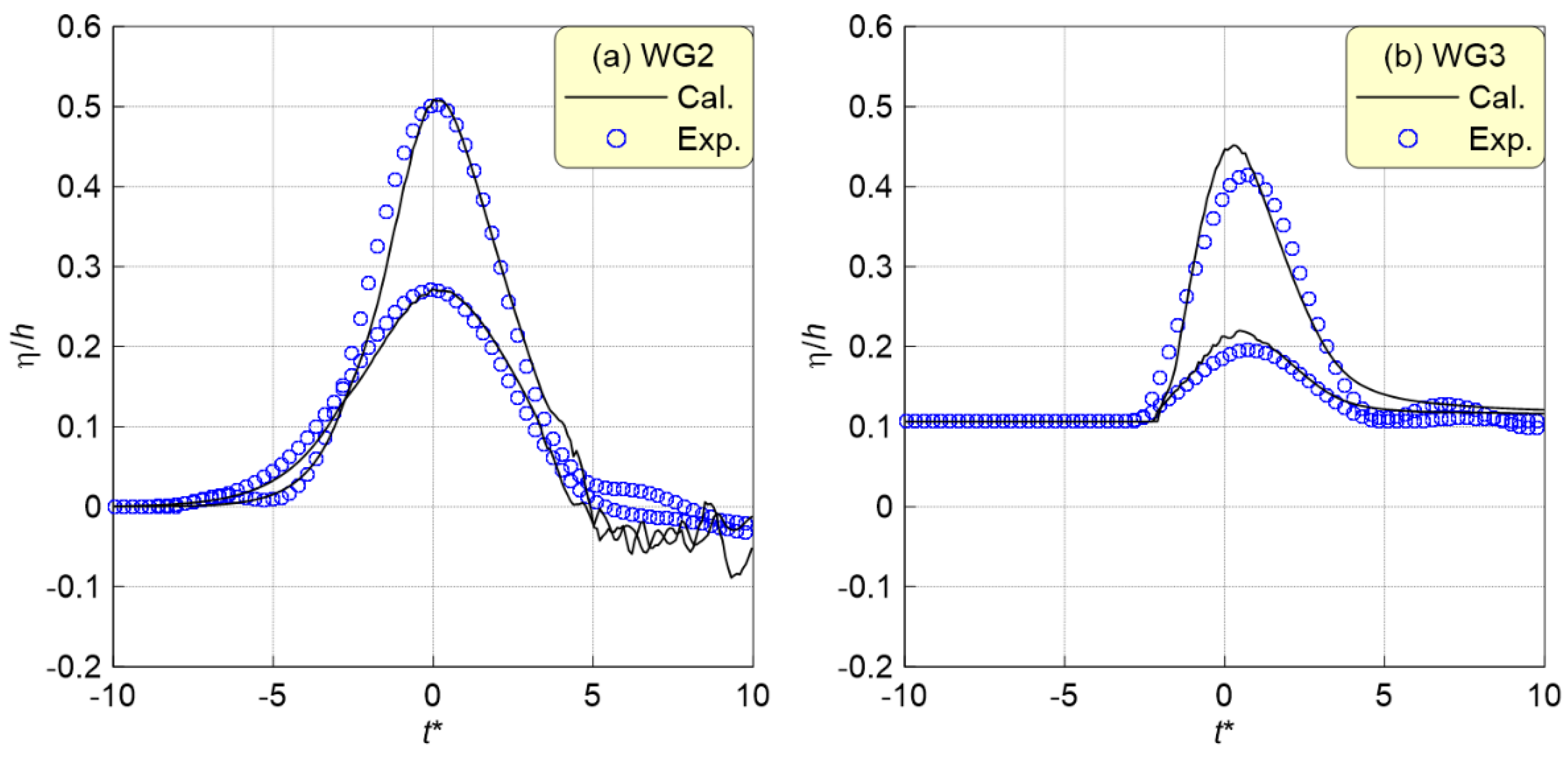
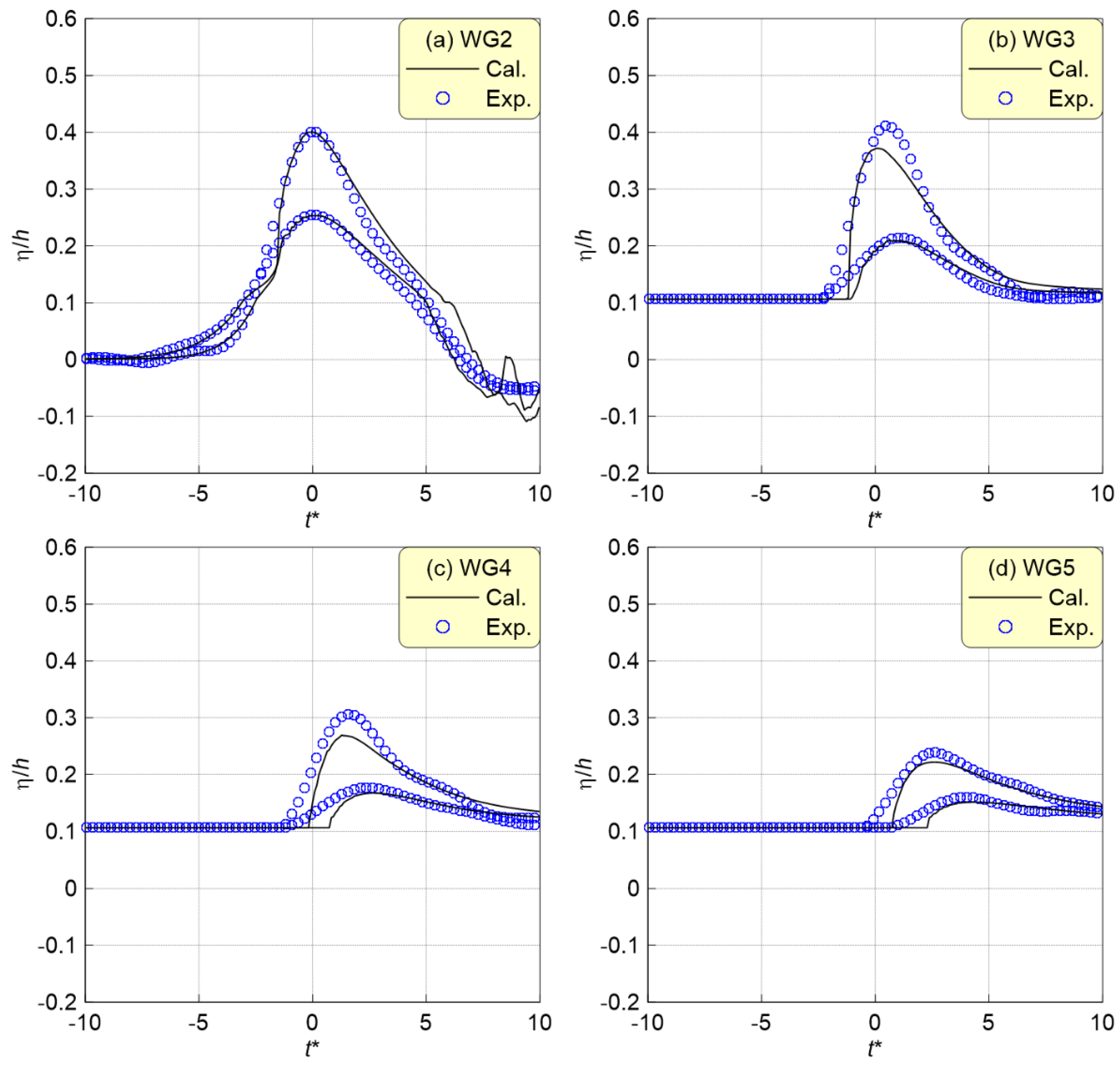
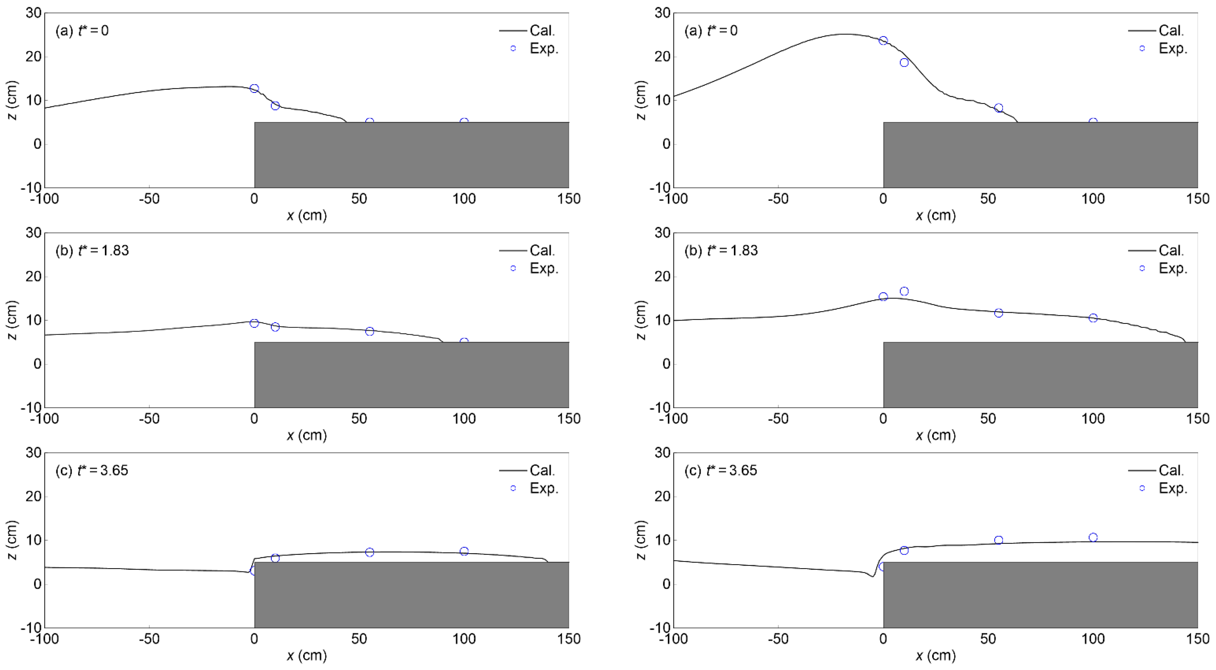
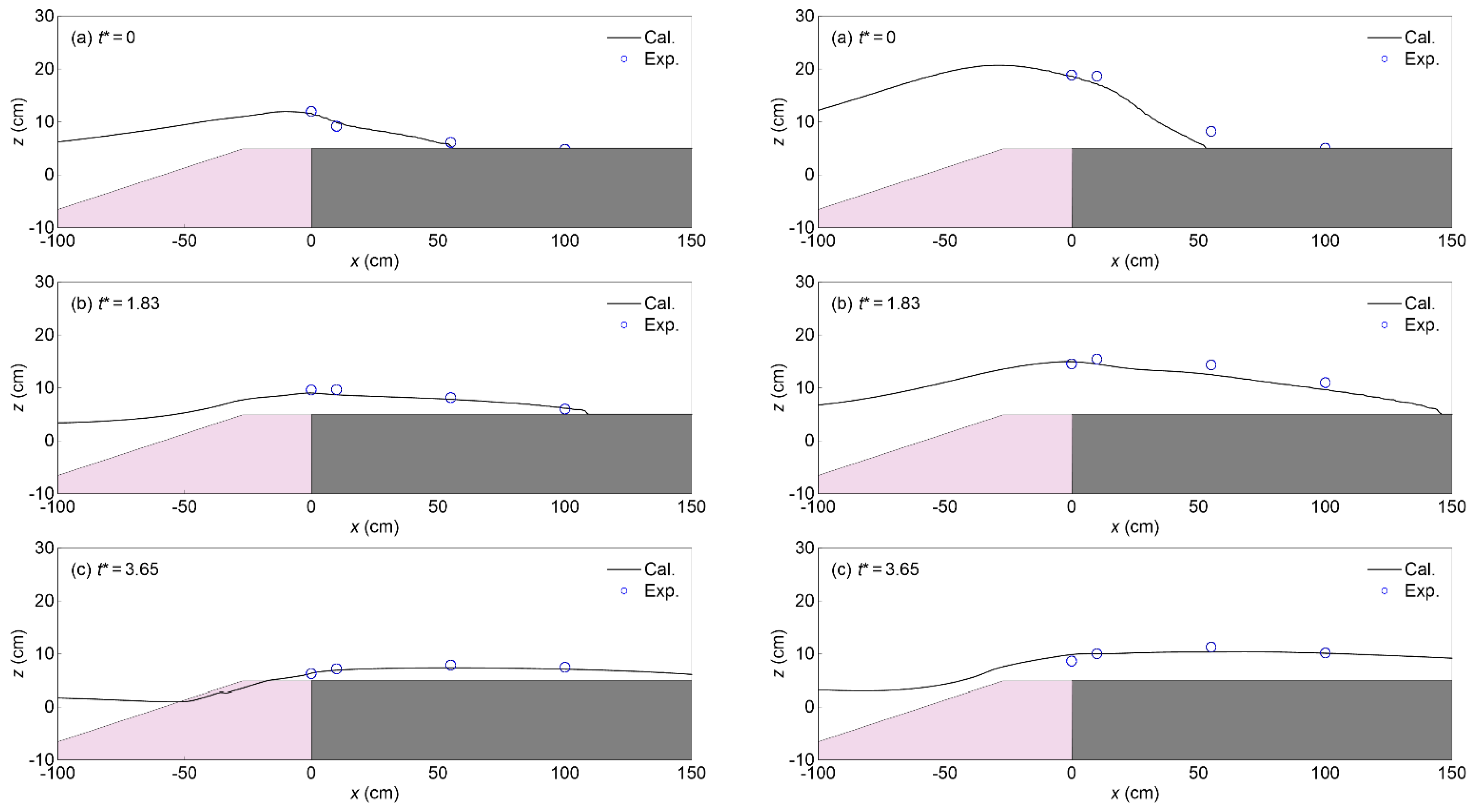
To verify the calculation accuracy of the NWT and validity of the analysis results, the water surface elevation distributions in front of the vertical wall and in the land area, measured in the physical modeling test, are compared in Figure 10, Figure 11, Figure 12 and Figure 13. Figure 10 and Figure 11 show the water surface elevation time distributions in the land area for the solitary wave conditions Run-4 ($A_0=8.2 \mathrm{cm}$, $\epsilon =0.18$) and Run-10 ($A_0=18.7 \mathrm{cm}$, $\epsilon =0.4$), and Figure 12 and Figure 13 show the spatial waveforms. Figure 10 and Figure 12 show the results for the VR, and Figure 11 and Figure 13 show the results for the WAR. The water surface elevation of the NWT is estimated as shown in Equation (19) by using the VOF function ($0\le F\le 1$).

$$\eta \left(t\right)={{\displaystyle \sum }}_{k=2}^{k=k_{max}-1}{F}_k{\mathsf{\Delta }\mathrm{z}}_k-h,$$

(19)

where $k=1$ and $k=k_{max}$ are the bottom and top boundaries of the NWT, respectively, and $\Delta z$ is the vertical grid size.

For the VR (Figure 10), the calculated values of the NWT reproduce the overall water surface elevation distributions accurately at WG3–WG5 in the land area, as well as the peak water surface elevation at WG2 directly in front of the vertical wall, during overtopping under the Run-4 and Run-10 conditions. For the WAR (Figure 11), the calculated water surface elevations in the NWT slightly underestimate the peak values at WG3, WG4, and WG5 in the land area. In addition, the NWT appropriately represents the water level distribution in the wave overtopping and inundation processes at WG2, as shown in Figure 10 and Figure 11a; however, an error resulted due to slight oscillations in water surface as the overtopping proceeded from the front of the revetment. Regarding the spatial distributions of the free water surface shown in Figure 12 and Figure 13, the NWT accurately reproduces the processes leading to inundation in the land area, including solitary wave overtopping, for the VR and WAR.

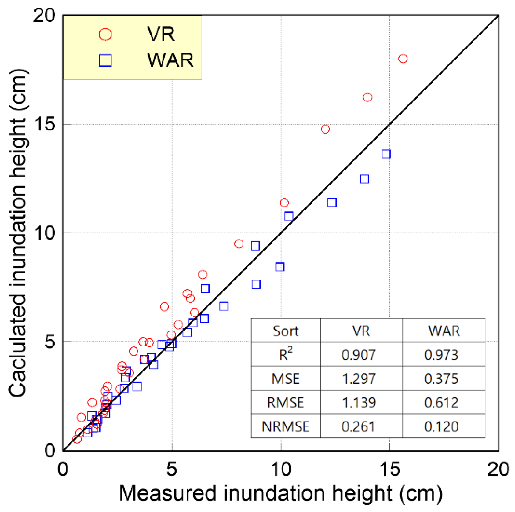
To evaluate the numerical accuracy of the NWT used in the solitary wave overtopping and inundation analysis according to the revetment type, this study used R-squared (R²), mean square error (MSE), root mean square error (RMSE), and normalized root mean square error (NRMSE), which are shown in Figure 14. The values of R², MSE, RMSE, and NRMSE are calculated as follows:

$${\mathrm{R}}^2=1-\frac{{\displaystyle \sum }{\left({\Omega }_i^{exp}-{\Omega }_i^{cal}\right)}^2}{{\displaystyle \sum }{\left({\Omega }_i^{exp}-\overline{{\Omega }^{exp}}\right)}^2},$$

(20)

$$\mathrm{MSE}=\frac{1}{N}{\displaystyle \sum }_{i=1}^N{\left({\Omega }_i^{exp}-{\Omega }_i^{cal}\right)}^2,$$

(21)

$$\mathrm{RMSE}=\sqrt{\frac{1}{N}{\displaystyle \sum }_{i=1}^N{\left({\Omega }_i^{exp}-{\Omega }_i^{cal}\right)}^2},$$

(22)

$$\mathrm{NRMSE}=\sqrt{\frac{{{\displaystyle \sum }}_{i=1}^N{\left({\Omega }_i^{exp}-{\Omega }_i^{cal}\right)}^2}{{{\displaystyle \sum }}_{i=1}^N{\left({\Omega }_i^{exp}\right)}^2}},$$

(23)

where ${\Omega }_i^{exp}$ is the measured value; ${\Omega }_i^{cal}$ is the calculated value; $\overline{{\Omega }^{exp}}$ is the mean value of ${\Omega }_i^{exp}$; and $N$ is the number of data points.

At WG3, WG4, and WG5, the calculated values from the NWT and measured values from the physical modeling test were compared at the maximum inundation height under 11 solitary wave conditions. The experimental values were slightly underestimated for the VR, whereas they tended to be overestimated for the WAR. Overall, the inundation height prediction accuracy was slightly higher for the WAR than for the VR based on the evaluations of R², MSE, RMSE, and NRMSE. Nevertheless, the accuracy of inundation analysis for the VR was considered to be at a reliable level.

Based on the above qualitative and quantitative verifications, we confirmed the validity and effectiveness of the NWT used in this study. Thus, we judged the solitary wave overtopping and inundation simulations in the NWT according to the revetment type as reliable.

5. Numerical Analysis Results

5.1. Wave Field and Flow Field

5.1.1. Overtopping and Inundation Process

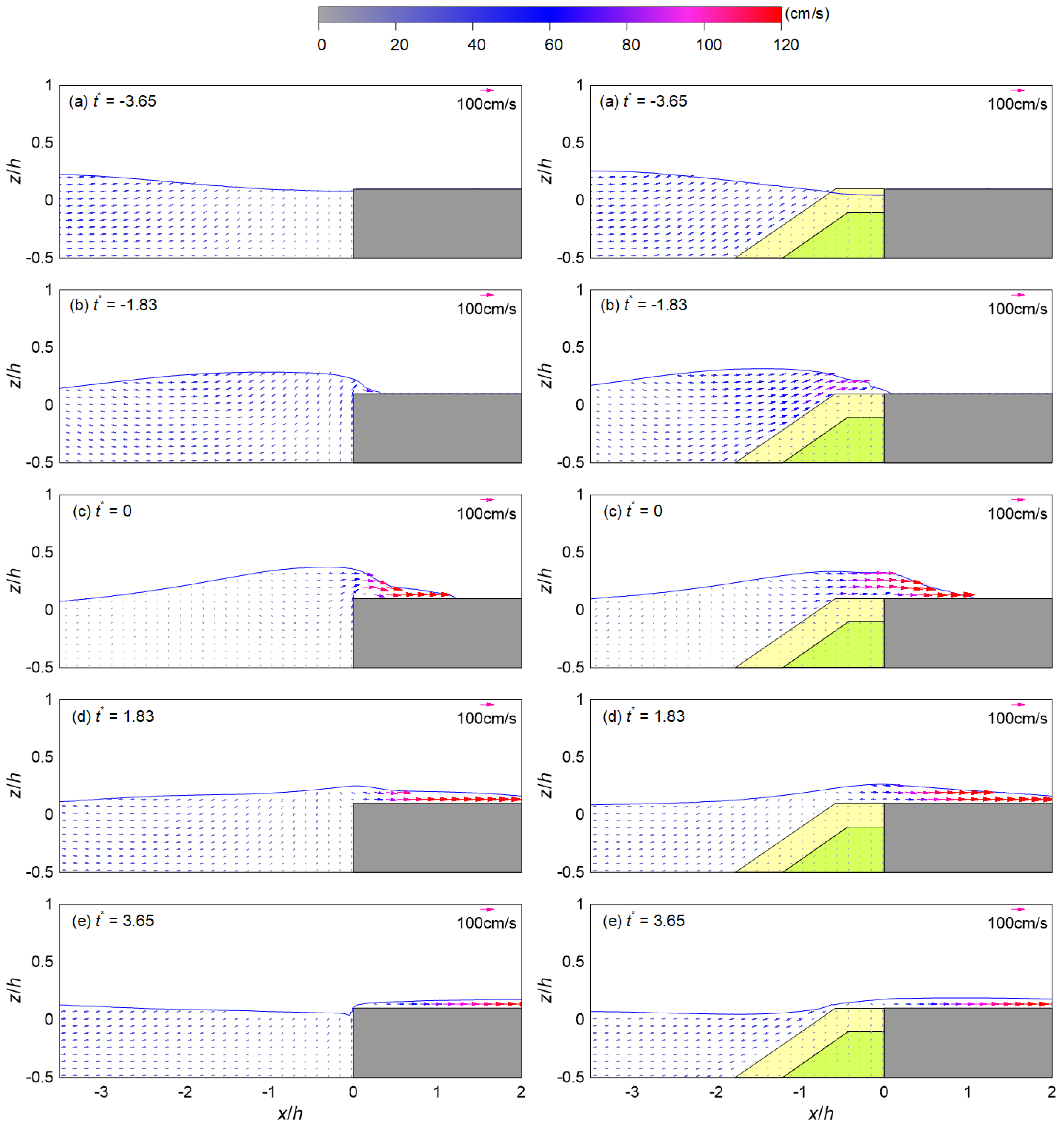
To compare the wave field and flow field changes in the solitary wave overtopping and inundation process at the VR and WAR, the representative incident conditions of Run-7 ($A_0=12.3 \mathrm{cm}$, $\epsilon =0.26$) are shown in Figure 15. In Figure 15c, $t^{*}=0$ indicates the moment the maximum water surface elevation occurs in front of the impermeable vertical wall at $x/h=0$; the wave and flow fields are shown at $\mathsf{\Delta }{t}^{*}=1.83$ intervals based on (c). The horizontal and vertical distances ($x$,$z$) are nondimensionalized using the depth $h$. In addition, the magnitude of the flow velocity can be determined from the vector scale and color scale.

In the results of the WAR shown on the right of Figure 15b, the flow cross-sectional area was reduced due to the wave absorber, causing the flow velocity of the solitary wave to significantly develop along the slope and the horizontal velocity to become dominant during the overtopping. The VR does not have a wave absorber. In the VR results on the left in Figure 15a, the horizontal velocity of the solitary wave is rapidly converted to vertical velocity owing to the blocking of the impermeable vertical wall, causing the water surface elevation to rise and overtopping to begin, as shown in Figure 15b. Additionally, for the VR on the left in Figure 15c, at the point where the maximum water surface elevation occurs at the edge of the vertical wall, flow separation occurs at the revetment crest because the solitary wave flow cannot bend by 90°. In contrast, for the WAR on the right of Figure 15, the flow passing through the wave absorber to the upper section is weak, and flow separation does not occur at the edge of the vertical wall because the horizontal flow is dominant above the crest.

5.1.2. Flow Field Distribution

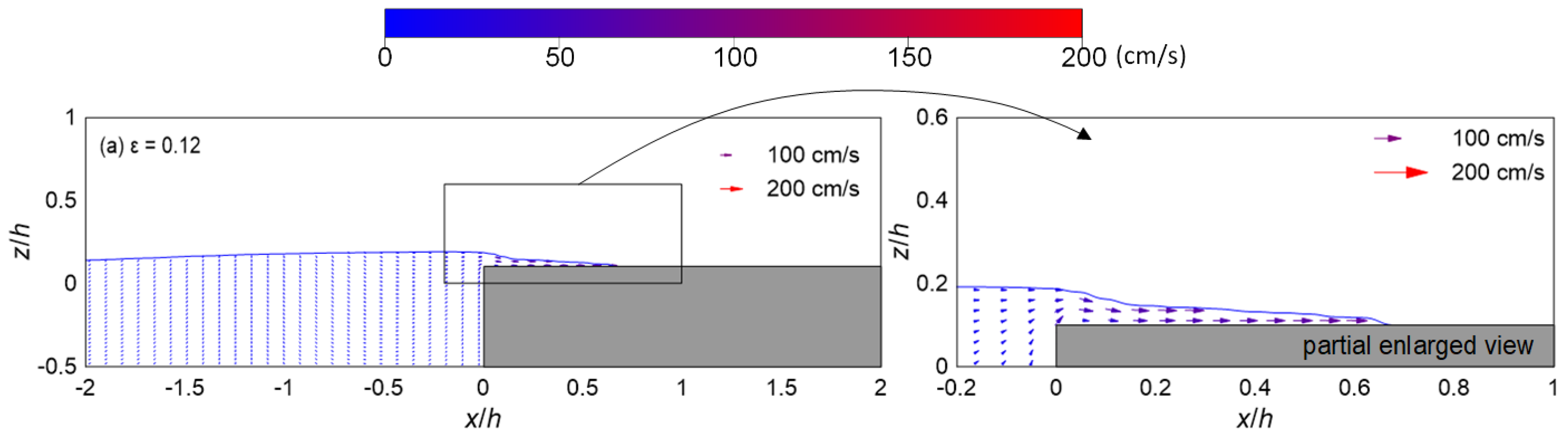
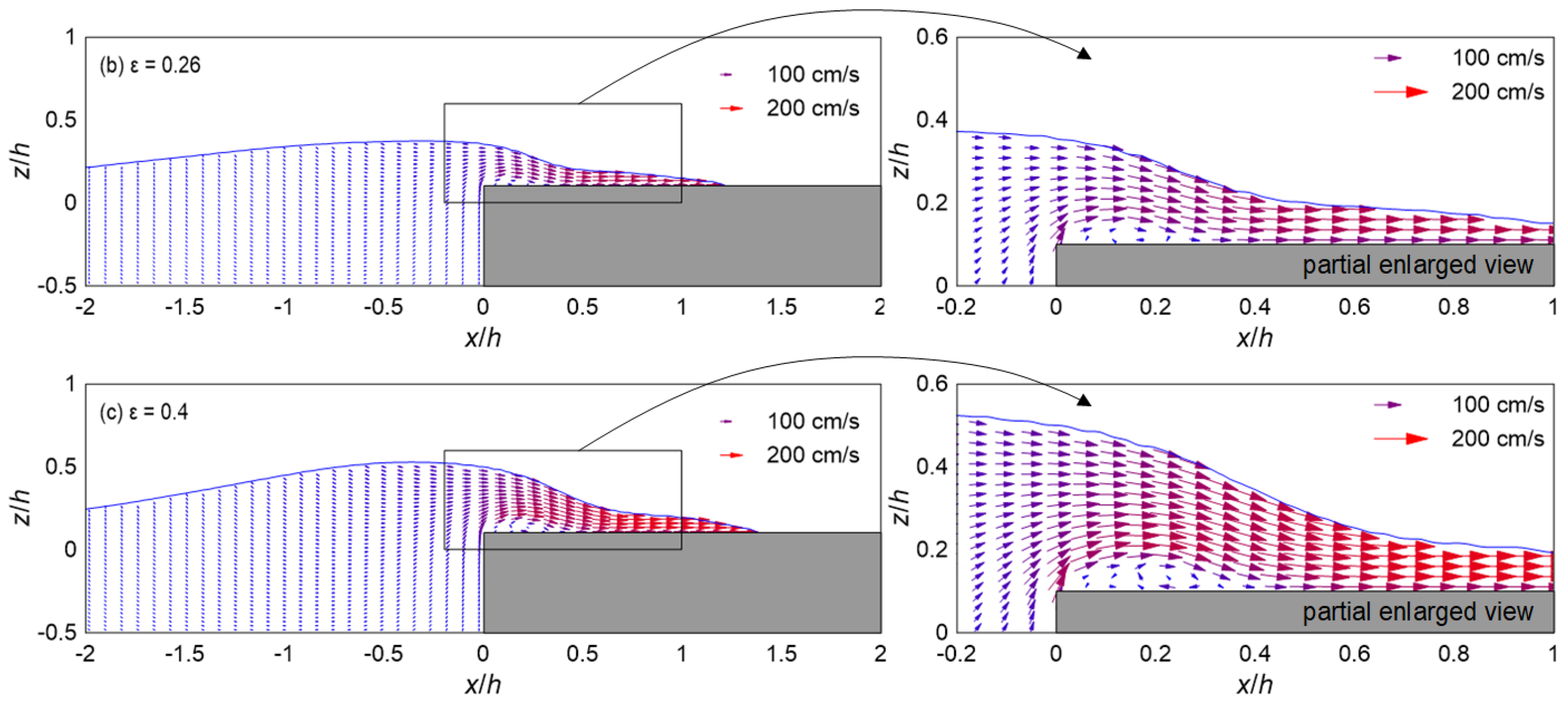
Figure 16 shows the wave and flow fields in detail at the point ($t^{*}=0$) when the maximum water surface elevation at $x/h=0$ (the edge of the vertical wall) in the VR, and Figure 17 shows the corresponding data for the WAR. The representative solitary wave conditions of Run-2 ($A_0=5.4 \mathrm{cm}$, $\epsilon =0.12$), Run-7 ($A_0=12.3 \mathrm{cm}$, $\epsilon =0.26$), and Run-10 ($A_0=18.7 \mathrm{cm}$, $\epsilon =0.4$) are shown in (a), (b), and (c), respectively.

When the solitary wave acts on the VR in Figure 16, the flow cannot bend sharply by 90° at the edge. Hence, flow separation occurs at the crest, and a separation region is formed. As $\epsilon$ increases, the flow velocity of the solitary wave increases, and it becomes difficult for the flow to sharply change its direction; this causes the flow separation to strengthen and the separation region to expand further. Consequently, the flow velocity of the separated flow is greater than that near the water surface, and the gradient of the spatial waveform of the solitary wave steepens. Moreover, a reversed flow gradient ($\frac{\partial u}{\partial z}$) may occur in the separation region owing to the reversed flow. For the WAR in Figure 17, the horizontal flow of the solitary wave is dominant above the wave absorber. Hence, in Figure 17c, where $\epsilon$ is large, flow separation does not occur. Thus, as observed in the experiment, the rise in water surface elevation at the VR, owing to the increase in the drag caused by the flow separation during overtopping, is larger than that at the WAR. In addition, at the WAR, with no sudden change in direction and no flow separation, the horizontal velocity is dominant during the inundation process, and the flow velocity gradient near the floor is smaller than that at the VR. The rise in water surface elevation during solitary wave overtopping and flow separation at the edge of the vertical wall during the inundation process is considered to greatly affect the solitary wave inundation in the land area.

5.2. Vertical Flow Velocity Distribution

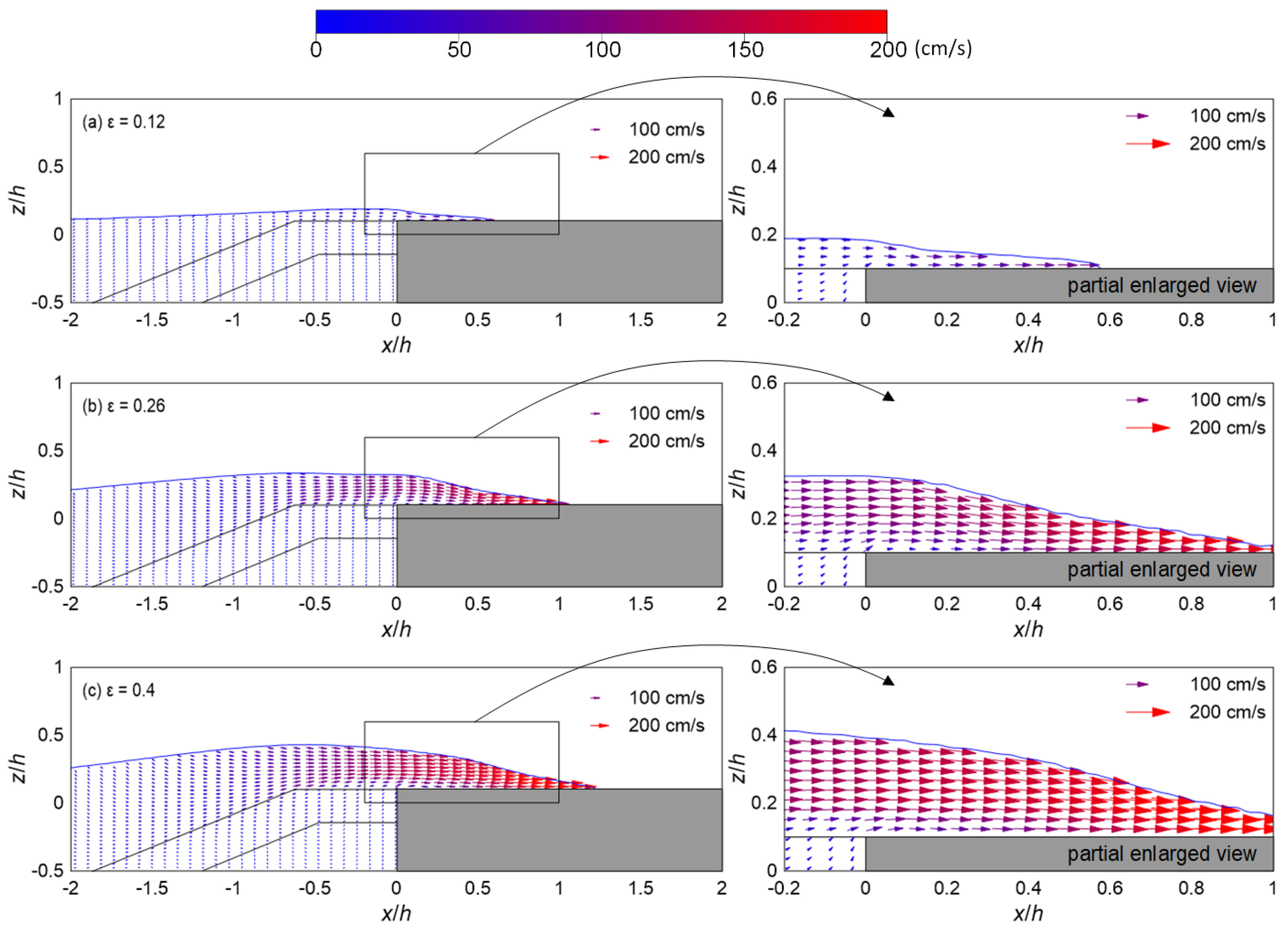
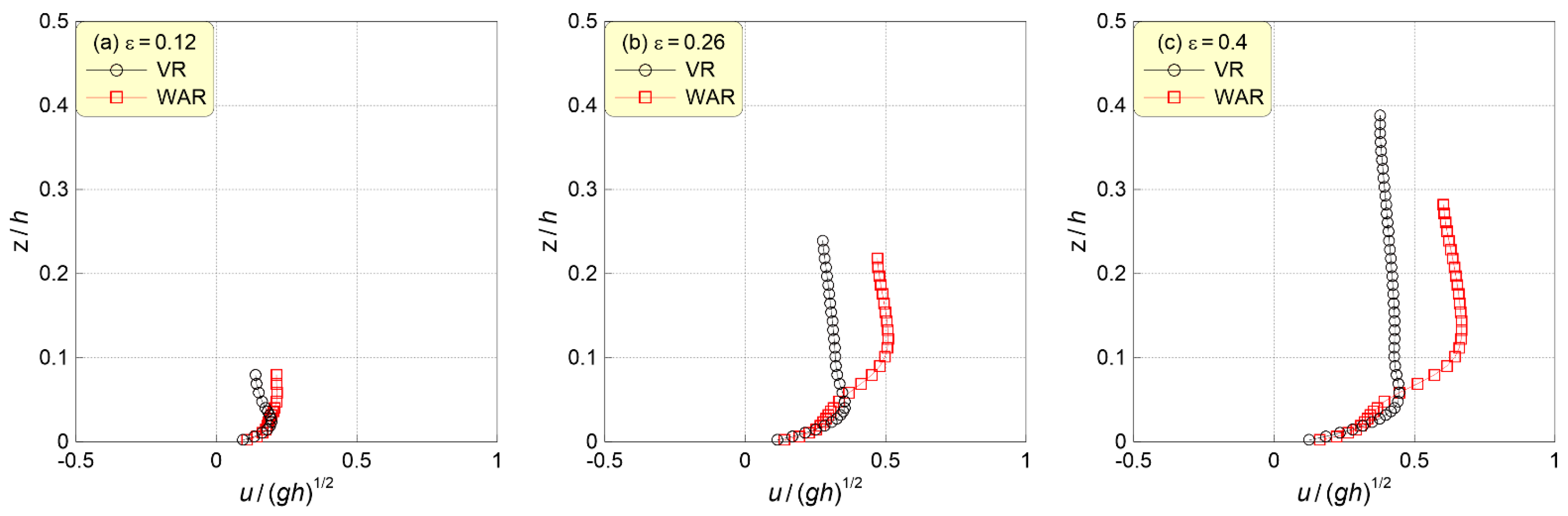
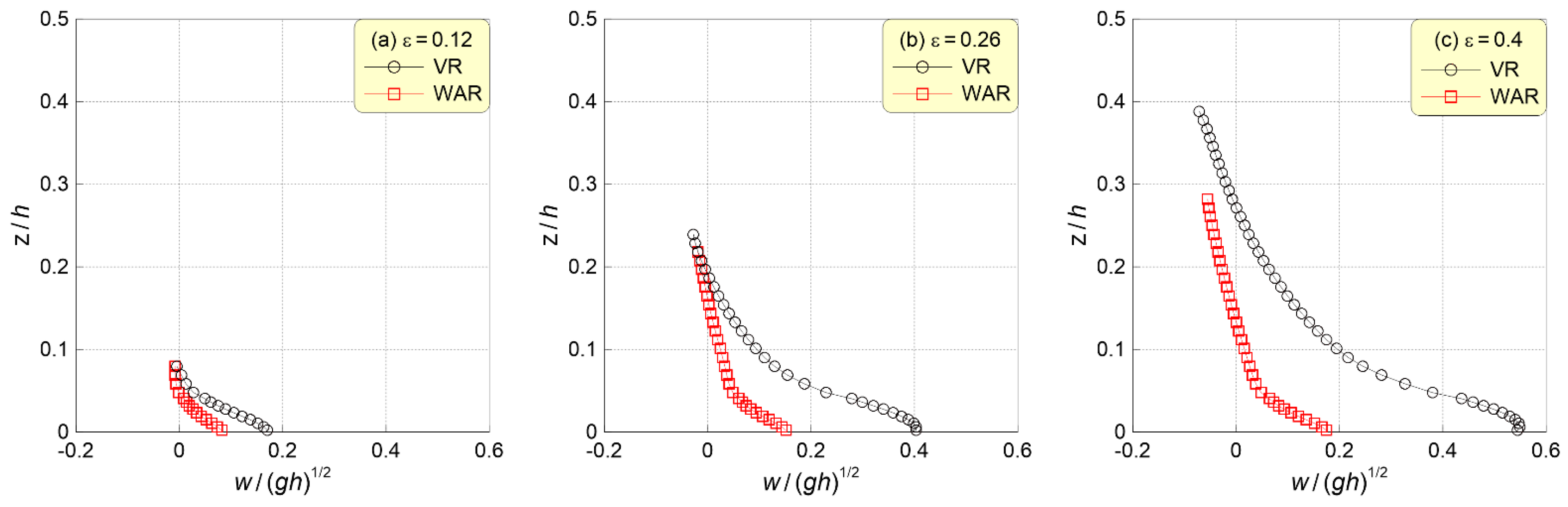
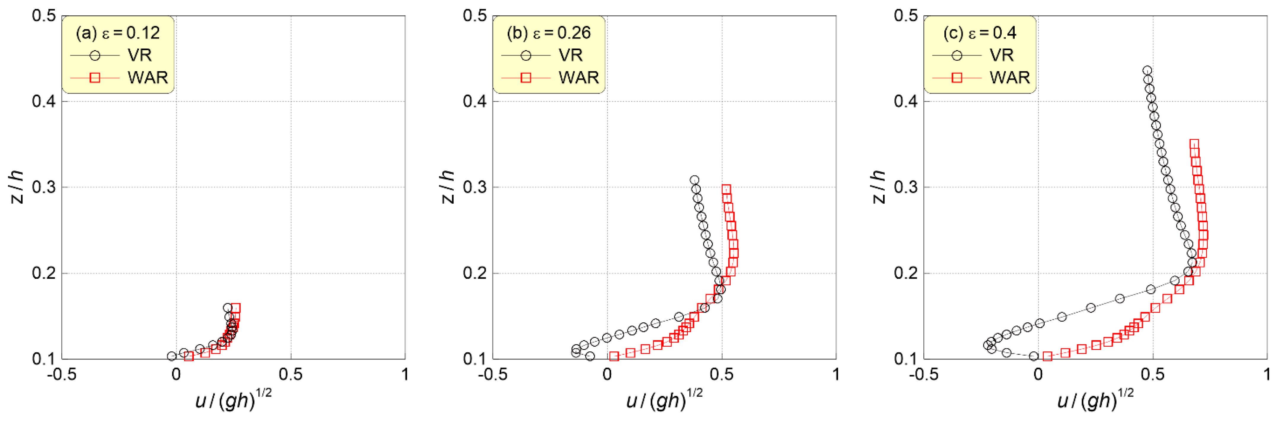
Figure 18 and Figure 19 show the vertical distributions of the horizontal and vertical velocity components ($u$, $w$) when the maximum water surface elevation occurs at the edge of the vertical wall at point $x/h=0$, and Figure 20 and Figure 21 show the corresponding data at the center of the flow separation region. The solitary wave conditions of Run-2 ($A_0=5.4 \mathrm{cm}$, $\epsilon =0.12$), Run-7 ($A_0=12.3 \mathrm{cm}$, $\epsilon =0.26$), and Run-10 ($A_0=18.7 \mathrm{cm}$, $\epsilon =0.4$) are shown in (a), (b), and (c), respectively. The flow velocity components on the vertical axes of the graphs are nondimensionalized by dividing them by the wave speed ($\sqrt{gh}$) of the shallow-water wave, and the $z$ direction on the horizontal axis is nondimensionalized using $h$.

As discussed for the wave and flow field section of the physical modeling test and numerical analysis, during solitary wave overtopping, the flow cross-sectional area gradually decreases along the slope of the wave absorber in the WAR, thus developing a horizontal velocity, which subsequently becomes dominant, as shown in Figure 17 and Figure 18. In contrast, at the VR, which consists of a vertical wall, the horizontal velocity of the solitary wave is converted to vertical velocity, and the upward flow dominates the flow in the propagation direction as overtopping occurs. Consequently, as shown in the physical modeling test, the rise in water surface elevation at the VR is larger than that at the WAR, and this trend intensifies as $\epsilon$ increases.

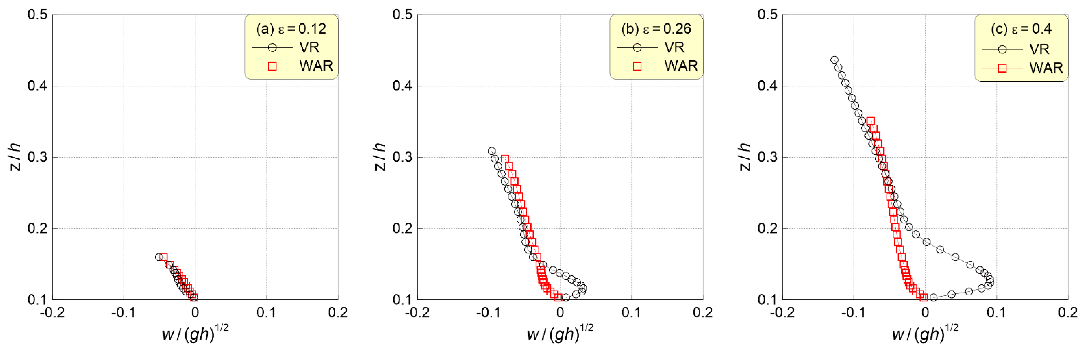
Further, in Figure 20 and Figure 21, which show the vertical distributions of the flow velocity at the center of the separation region, the separated flow that develops near the boundary of the separation region at the VR causes the largest horizontal velocity, which is shown in Figure 20b,c. In addition, $-u$ and $+w$ appear at the VR owing to the influence of the reversed flow. Conversely, at the WAR, the flow distribution of a typical open channel is observed. Furthermore, owing to the influence of the water surface gradient in the overtopping–inundation process of the solitary wave, $-w$ in the gravitational direction develops outside the separation region. At the VR, where the water surface gradient is steeper than that at the WAR, $-w$ develops to a greater extent near the water surface.

This flow velocity distribution at the VR will form strong vorticity opposite to the inside and boundary of the separation region and greatly differs from the observations at the WAR. This is also judged to have a strong influence on the solitary wave overtopping and inundation.

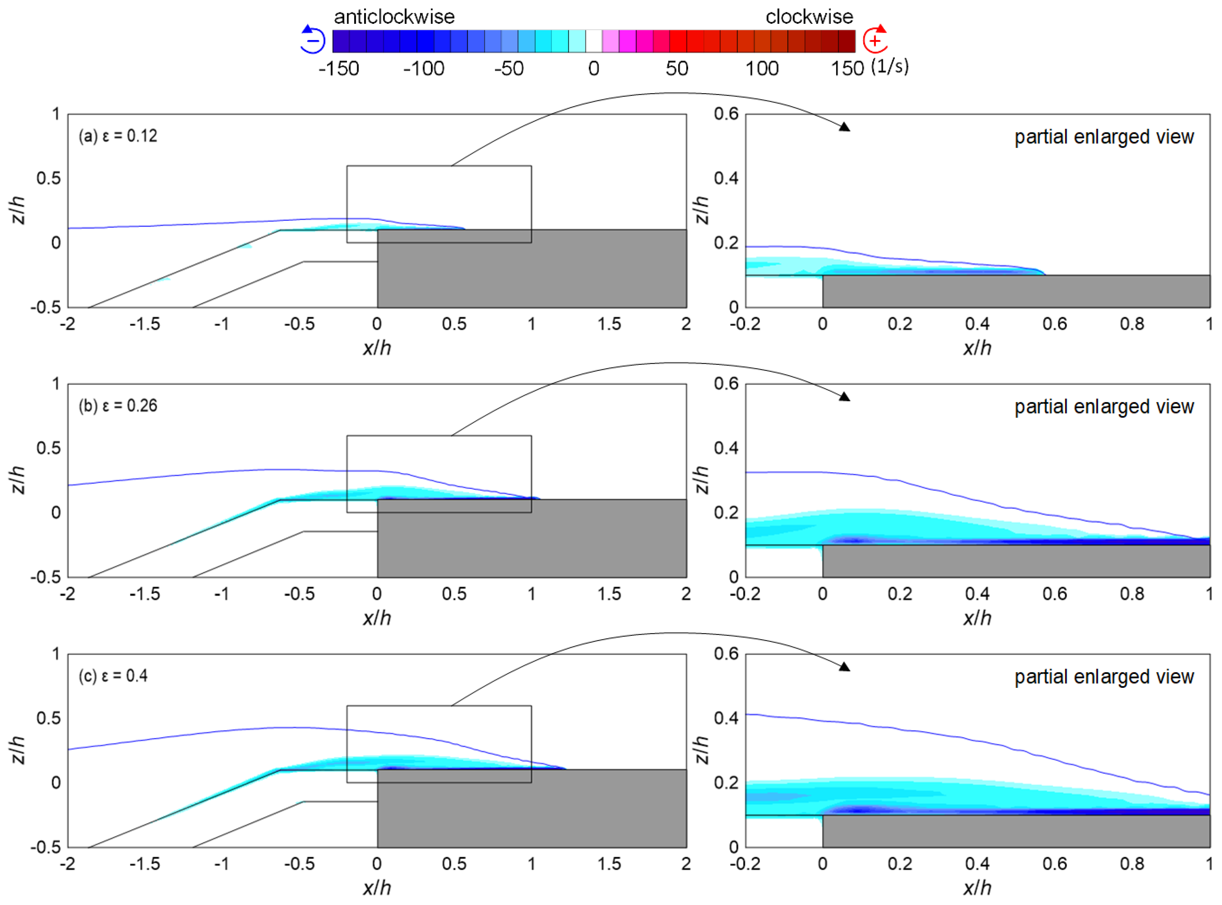
5.3. Vortex Field

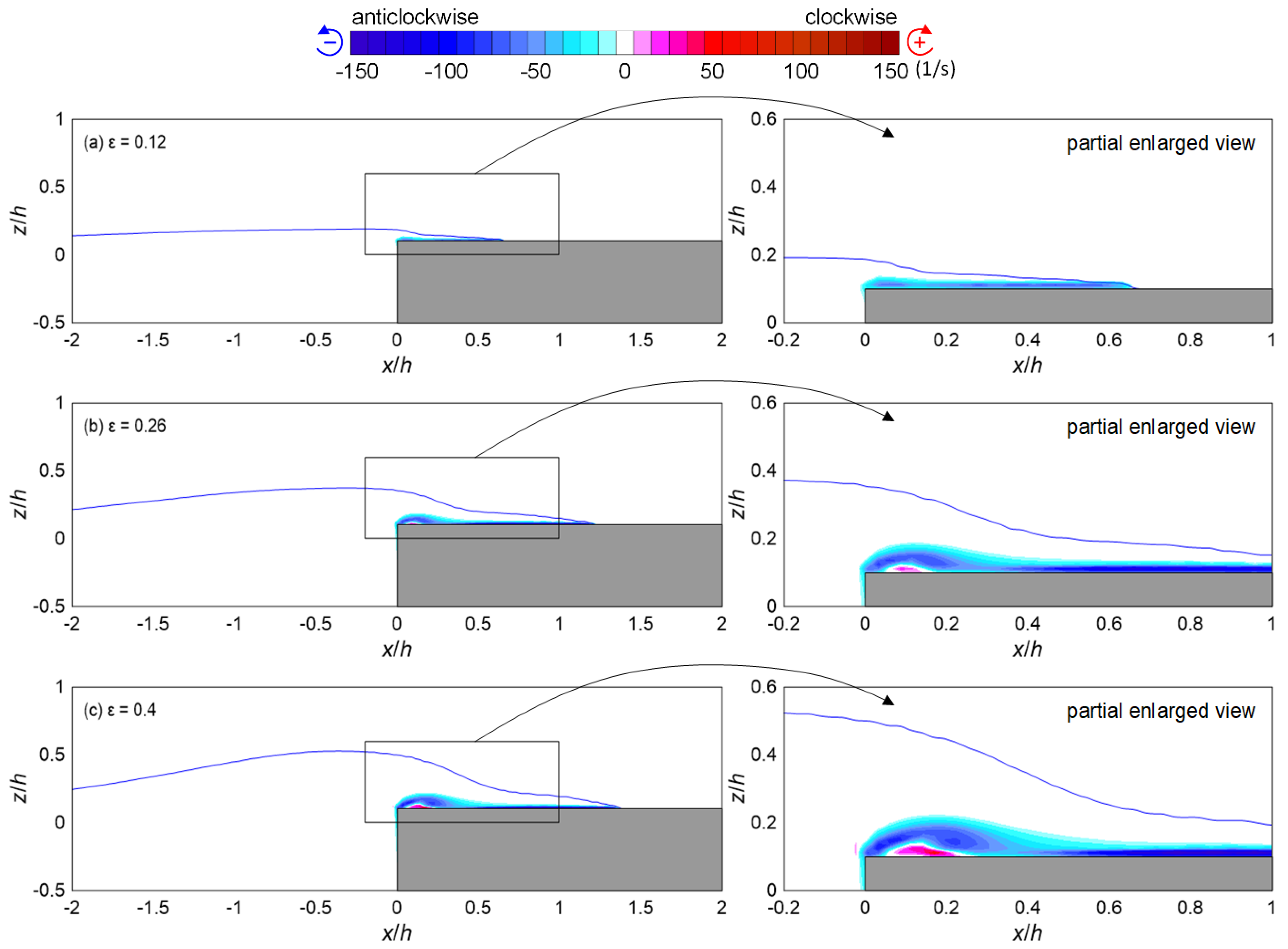
To analyze the vortex phenomenon in the solitary wave overtopping and inundation process at the VR and WAR, Figure 22 and Figure 23 show the vortex fields at $t^{*}=0$ when the maximum water surface elevation occurs at the vertical wall edge. The solitary wave incidence conditions of Run-2 ($A_0=5.4 \mathrm{cm}$, $\epsilon =0.12$), Run-7 ($A_0=12.3 \mathrm{cm}$, $\epsilon =0.26$), and Run-10 ($A_0=18.7 \mathrm{cm}$, $\epsilon =0.4$) are shown in (a), (b), and (c), respectively. The vorticity (${\zeta }_{ij}$) is indicated in color; the red line indicates clockwise vorticity $+{\zeta }_{ij}$, and the blue line indicates counterclockwise vorticity $-{\zeta }_{ij}$. Here, ${\zeta }_{ij}$ is calculated as follows:

$${\zeta }_{ij}=\frac{\partial v_j}{\partial x_i}-\frac{\partial v_i}{\partial x_j}.$$

(24)

Generally, because the flow velocity of the solitary wave increases as $\epsilon$ increases, a strong $-{\zeta }_{ij}$ tends to occur owing to friction at the floor of the revetment, as shown in Figure 22 and Figure 23. At the VR where flow separation occurs (Figure 22), as $\epsilon$ increases, reversed flow develops in the separation region, and $+{\zeta }_{ij}$ strengthens. Additionally, $-{\zeta }_{ij}$ at the boundary of the separation region, caused by the developing separated flow, becomes stronger as $\epsilon$ increases. This strong vortex phenomenon can dissipate the kinetic energy of the solitary wave and slow down the inundation of the land area. Further, at the WAR where flow separation does not occur (Figure 23), there are no unusual vortex phenomena except those near the floor of the revetment and the wave absorber surface.

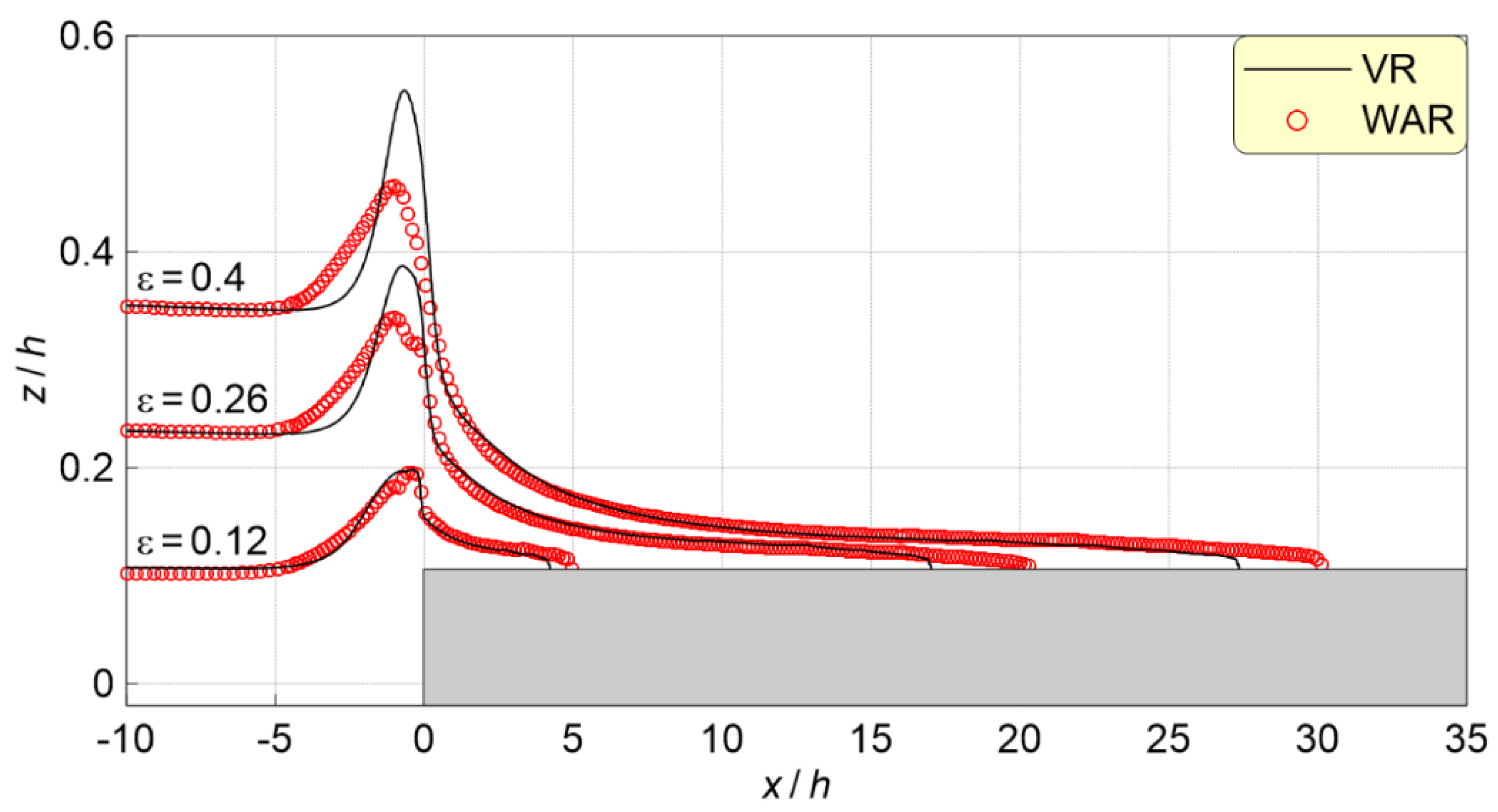
5.4. Maximum Water Surface Elevation Distribution

As in Figure 15, Figure 24 shows the spatial distribution of the maximum water surface elevation generated during the solitary wave overtopping and inundation process at the VR and WAR. The representative solitary wave conditions of Run-2 ($A_0=5.4 \mathrm{cm}$, $\epsilon =0.12$), Run-7 ($A_0=12.3 \mathrm{cm}$, $\epsilon =0.26$), and Run-10 ($A_0=18.7 \mathrm{cm}$, $\epsilon =0.4$) are shown in the graphs.

As in the physical modeling results, the difference in the maximum water surface elevation at the point $x/h=0$ at the edge of the vertical wall between the VR and WAR was not large under Run-2 conditions where $\epsilon$ is small and the effective wavelength is long. Under Run-7 and Run-10 conditions, the maximum overtopping water surface elevation at the vertical wall was larger at the VR than at the WAR, and as $\epsilon$ increased, the difference in water surface elevation tended to increase. At the VR, this can be explained by the rise in water surface elevation caused by the flow separation at the revetment crest and the conversion of the horizontal velocity of the solitary wave to vertical velocity due to the sharp decrease in the cross-sectional area because of the vertical wall, as discussed in the physical modeling test and numerical analysis. At the WAR, because the flow cross-sectional area gradually decreases along the gradient of the wave absorber, the horizontal velocity of the solitary wave becomes dominant as overtopping progresses, and the rise in water surface elevation is not large. Hence, near the shore, although the maximum inundation height is large at the VR ($I_H^{\mathrm{VR}}>I_H^{\mathrm{WAR}}$), as the wave propagates inland, the difference ($\Delta I_H$) decreases, and the height at the WAR increases ($I_H^{\mathrm{VR}}<I_H^{\mathrm{WAR}}$); however, this difference is not large.

The inundation distance was observed to be longer at the WAR than at the VR. This was partly because the horizontal velocity is dominant during solitary wave overtopping; however, at the VR, energy damping owing to vortex generation caused by flow separation also had a substantial effect.

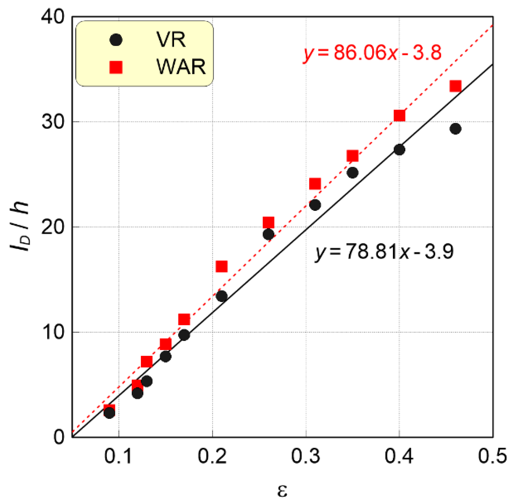
5.5. Inundation Distance

Figure 25 shows a graph of the inundation distance ($I_D$) of the solitary wave according to $\epsilon$ at the VR and WAR, nondimensionalized using the depth ($h$), and

Table 3. Inundation distances due to $\epsilon$.

$\mathit{\epsilon }$	$\mathbf{Inundation} \mathbf{Distance} {\mathit{I}}_{\mathit{D}} \mathbf{\left(}\mathbf{cm}\mathbf{\right)}$		$\mathbf{\Delta }{\mathit{I}}_{\mathit{D}} \mathbf{\left(}\mathbf{cm}\mathbf{\right)}$	$\mathbf{\Delta }{\mathit{I}}_{\mathit{D}}\mathbf{/}\mathit{h}$	${\mathit{I}}_{\mathit{D}}\mathbf{/}\mathit{h}$		${\mathit{I}}_{\mathit{D}}^{\mathbf{W}\mathbf{A}\mathbf{R}}\mathbf{/}{\mathit{I}}_{\mathit{D}}^{\mathbf{V}\mathbf{R}}$
	${\mathit{I}}_{\mathit{D}}^{\mathbf{V}\mathbf{R}}$	${\mathit{I}}_{\mathit{D}}^{\mathbf{W}\mathbf{A}\mathbf{R}}$	${\mathit{I}}_{\mathit{D}}^{\mathbf{W}\mathbf{A}\mathbf{R}}\mathbf{-}{\mathit{I}}_{\mathit{D}}^{\mathbf{V}\mathbf{R}}$		${\mathit{I}}_{\mathit{D}}^{\mathbf{V}\mathbf{R}}\mathbf{/}\mathit{h}$	${\mathit{I}}_{\mathit{D}}^{\mathbf{W}\mathbf{A}\mathbf{R}}\mathbf{/}\mathit{h}$
0.09	109.25	121.5	12.25	0.26	2.32	2.59	1.11
0.12	197.5	231.5	34	0.72	4.20	4.93	1.17
0.13	250.2	338.5	88.3	1.88	5.32	7.20	1.35
0.15	361.5	415.5	54	1.15	7.69	8.84	1.15
0.17	458.5	526.5	68	1.45	9.76	11.20	1.15
0.21	631.5	762.5	131	2.79	13.44	16.22	1.21
0.26	906.5	958.5	52	1.11	19.29	20.39	1.06
0.31	1038.5	1132.5	94	2.00	22.10	24.10	1.09
0.35	1183.5	1258.5	75	1.60	25.18	26.78	1.06
0.4	1284.5	1437.5	153	3.26	27.33	30.59	1.12
0.46	1378.5	1570.5	192	4.09	29.33	33.41	1.14
Mean value (cm)			86.69	1.84	Mean value		1.15

shows the inundation data. The superscript VR or WAR next to $I_D$ indicates the type of revetment.

As the incident wave height of the solitary wave increases (as $\epsilon$ increases), the inundation distance increases almost linearly. There are two reasons why the inundation distance at the VR is smaller than that at the WAR. First, at the WAR, the horizontal velocity caused by the gradual reduction in the flow cross-sectional area during solitary wave overtopping is dominant, which affects the inundation process. Second, at the VR, the drag increases owing to flow separation near the edge of the vertical wall, and energy dissipates owing to the vortexes.

Hence, a difference ($\Delta I_D=I_D^{\mathrm{WAR}}-I_D^{\mathrm{VR}}$) occurs between the inundation distances of VR and WAR ($I_D^{\mathrm{VR}} \mathrm{and} I_D^{\mathrm{WAR}}$), which increases as $\epsilon$ increases. Under the condition of $\epsilon =0.46$, for which the incident wave height of the solitary wave is the largest, the largest difference of $\Delta I_D=192 \mathrm{cm}$, $\Delta I_D/h=4.09$ occurs. Additionally, under the $\epsilon =0.13$ condition, the ratio difference is the largest at $\Delta I_D=88.3 \mathrm{cm}$, $\Delta I_D/h=1.88$, and $I_D^{\mathrm{VR}}$ becomes 35% larger than $I_D^{\mathrm{WAR}}$. On average, $\Delta I_D=86.69 \mathrm{cm}$, $\Delta I_D/h=1.84$, and $I_D^{\mathrm{WAR}}/I_D^{\mathrm{VR}}$ is $1.06–1.35$. Thus, the average inundation distance is 15% longer at the WAR than at the VR.

6. Discussion

In the results of the physical modeling test, the difference in inundation height in the land area according to revetment type was not clearly explained. Here, we will comprehensively discuss the aspects that were not explained earlier, along with the results of the numerical analysis.

In Figure 7a, the inundation height is larger at the WAR when $\epsilon <0.3$ for the solitary wave, whereas it is larger at the VR when $\epsilon >0.3$ at WG3 ($x/h=0.21$). This is because, as shown in Figure 14, the vertical velocity of the solitary wave developed along the vertical wall of the VR increases the water surface elevation, and a rapid drop in the water surface elevation occurs as the horizontal velocity is converted at the revetment crest. Conversely, at the WAR, where the horizontal velocity is dominant during the overtopping, the drop in water surface elevation at the revetment crest is not large. Because the flow separation near the revetment edge increases the drag in this process, the sharp drop in the water surface elevation is delayed (see Figure 15 and Figure 21). Hence, as $\epsilon$ decreases, the flow separation weakens, and the inundation height at the WAR becomes larger than that at the VR; as $\epsilon$ increases, the flow separation strengthens, and the separation region expands, which causes the inundation height at the VR to increase.

The maximum inundation height at WG4 ($x/h=1.17$) increases to a greater extent at the WAR with an increase in $\epsilon$ (see Figure 14b). As evidenced in Figure 15 and Figure 21, because the point $x/h=1.17$ at the VR is outside the flow separation region, as the drag resistance disappears, the flow velocity increases, and the water surface elevation drops sharply. Hence, in the numerical analysis results of Figure 23 and in the physical modeling test, as $\epsilon$ increases at the point $x/h=1.17$, the inundation height at the WAR increases to a greater extent than at the VR.

As shown in Figure 14c, the difference in inundation height between the VR and WAR at WG5 ($x/h=2.13$) is not large. A comparison of Figure 15 and Figure 16 shows that the solitary wave field and flow field near the shore, which exhibit complex flow phenomena, greatly differ between the VR and WAR. However, as the solitary wave propagates inland, its flow stabilizes, and as the water surface elevation drops, the difference in inundation height between the VR and WAR becomes small.

7. Conclusions

This study conducted a physical modeling test and numerical analysis to investigate the phenomena of wave overtopping and inundation according to the revetment type for solitary waves. In the physical modeling test, we constructed a VR and WAR and measured the water surface elevations during the overtopping and inundation process of the solitary wave. In the numerical analysis, we constructed the same revetments in an NWT as in the experiment and analyzed the wave fields, flow fields, and vortex fields in the solitary wave overtopping and inundation process.

In the physical modeling test, the maximum water level at the front of the revetment showed similar results for the VR and WAR under the condition of small wave height (Run-1) when a solitary wave overtopped. However, as the height of the wave increased, the maximum water level was larger at the VR than at WAR, and the difference in maximum water level tended to increase. In contrast with the results at the front of the revetment, a reversal occurred, in which the maximum inundation height increased at the WAR than at VR as the wave propagated inland. To confirm the validity and effectiveness of the NWT wave generation method, we compared and reviewed the approximate waveform of the solitary wave and flow velocity. In addition, the time waveforms and spatial waveforms calculated in the NWT accurately reproduced the water surface elevations measured by the WGs in the experimental tank. As the flow velocity of the solitary wave cannot bend at right angles at the VR, flow separation occurred at the revetment crest, and a separation region was formed. Conversely, at the WAR, the flow cross-sectional area gradually decreased along the slope of the wave absorber, leading to typical open channel flow characteristics in which the horizontal velocity was dominant during overtopping and inundation. At the WAR where flow separation did not occur, strong vorticity developed only in the boundary layer owing to floor friction. However, at the VR where flow separation occurred, strong vorticity and separated flows occurred inside and at the boundary of the separation region. Owing to the increase in drag, generation of vorticity, and energy damping due to flow separation at the VR crest, as well as the development of horizontal velocity on the slope of the inclined wave absorber at the WAR, the inundation distance was longer at the WAR than at the VR. As ε increased, the inundation distance of the solitary wave increased; the difference in inundation distance between the VR and WAR also tended to increase. The difference in the average inundation distance of the solitary waves was 86.69 cm, and inundation progressed by an average of 15% further inland in the case of the WAR than the VR.

WAR structures are known to reduce damage from overtopping and inundation caused by periodic waves more effectively than VR. However, this study on solitary waves yielded experimental and numerical results that were contrary to general knowledge. It is judged that the analysis result of inundation characteristics according to the revetment type can be used for responding to secondary damage such as inundation and collision caused by tsunamis. In addition, it can be concluded that sufficient distance and slope for energy dissipation are necessary when sloped revetment is applied to reduce wave overtopping and inundation for long period waves such as solitary waves.

This study analyzed wave overtopping and inundation characteristics according to the type of structure and was limited to solitary waves. However, analyzing the hydraulic phenomena of the tsunami is difficult, as the actual tsunami is wider than the solitary waveform. Tsunami-like waves [13] and N-solitary waves [53,54,55,56], which have hydraulic phenomena similar to tsunamis, are being actively researched. To improve the reliability of this research, we plan to conduct physical modeling tests and numerical analyses in the future by applying WARs of various structural types to solitary waves or tsunami-like waves.

References

- Synolakis, C.E. The runup of solitary waves. J. Fluid Mech. 1987, 185, 523–545. [Google Scholar] [CrossRef]
- Grilli, S.T.; Subramanya, R.; Svendsen, I.A.; Veeramony, J. Shoaling of solitary waves on plane beaches. J. Waterw. Port Coast. Ocean Eng. 1994, 120, 609–628. [Google Scholar] [CrossRef] [Green Version]
- Li, Y.; Raichlen, F. Non-breaking and breaking solitary wave run-up. J. Fluid Mech. 2002, 456, 295–318. [Google Scholar] [CrossRef] [Green Version]
- Chang, Y.-H.; Hwang, K.-S.; Hwung, H.-H. Large-scale laboratory measurements of solitary wave inundation on a 1:20 slope. Coast. Eng. 2009, 56, 1022–1034. [Google Scholar] [CrossRef]
- Hwang, K.-S.; Chang, Y.-H.; Hwung, H.-H.; Li, Y.-S. Large scale experiments on evolution and run-up of breaking solitary waves. J. Earthq. Tsunami 2007, 1, 257–272. [Google Scholar] [CrossRef]
- Hsiao, S.C.; Lin, T.C. Tsunami-like solitary waves impinging and overtopping an impermeable seawall: Experiment and RANS modeling. Coast. Eng. 2010, 57, 1–18. [Google Scholar] [CrossRef]
- Jervis, M.; Peregrine, D.H. Overtopping of waves at a wall: A theoretical approach. In Proceedings of the 25th International Conference on Coastal Engineering, American Society of Civil Engineers, Orlando, FL, USA, 2–6 September 1997; pp. 2192–2205. [Google Scholar]
- Hunt-Raby, A.C.; Borthwick, A.G.L.; Stansby, P.K.; Taylor, P.H. Experimental measurement of focused wave group and solitary wave overtopping. J. Hydraul. Res. 2011, 49, 450–464. [Google Scholar] [CrossRef] [Green Version]
- Baldock, T.E.; Peiris, D.; Hogg, A.J. Overtopping of solitary waves and solitary bores on a plane beach. Proc. Royal Soc. A Math. Phys. Eng. Sci. 2012, 468, 3494–3516. [Google Scholar] [CrossRef] [Green Version]
- Lin, T.-C.; Hwang, K.-S.; Hsiao, S.-C.; Yang, R.-Y. An experimental observation of a solitary wave impingement, run-up and overtopping on a seawall. J. Hydrodyn. Ser. B 2012, 24, 76–85. [Google Scholar] [CrossRef]
- Huber, L.E.; Evers, F.M.; Hager, W.H. Solitary wave overtopping at granular dams. J. Hydraul. Res. 2017, 55, 799–812. [Google Scholar] [CrossRef]
- Jiang, C.; Liu, X.; Yao, Y.; Deng, B.; Chen, J. Numerical investigation of tsunami-like solitary wave interaction with a seawall. J. Earthq. Tsunami 2017, 11, 1740006. [Google Scholar] [CrossRef]
- Lee, W.-D.; Yeom, G.-S.; Kim, J.; Lee, S.; Kim, T. Runup characteristics of a tsunami-like wave on a slope beach. Ocean Eng. 2022, 259, 111897. [Google Scholar] [CrossRef]
- Rueben, M.; Holman, R.; Cox, D.; Shin, S.; Killian, J.; Stanley, J. Optical measurements of tsunami inundation through an urban waterfront modeled in a large-scale laboratory basin. Coast. Eng. 2011, 58, 229–238. [Google Scholar] [CrossRef]
- Shin, S.; Lee, K.-H.; Park, H.; Cox, D.T.; Kim, K. Influence of a infrastructure on tsunami inundation in a coastal city: Laboratory experiment and numerical simulation. Coast. Eng. Proc. 2012, 1, 8. [Google Scholar] [CrossRef]
- Park, H.; Cox, D.T.; Lynett, P.J.; Wiebe, D.M.; Shin, S. Tsunami inundation modeling in constructed environments: A physical and numerical comparison of free-surface elevation, velocity, and momentum flux. Coast. Eng. 2013, 79, 9–21. [Google Scholar] [CrossRef]
- Kim, D.-H.; Lynett, P.; Socolofsky, S.A. A depth-integrated model for weakly dispersive, turbulent, and rotational fluid flows. Ocean Model. 2009, 27, 198–214. [Google Scholar] [CrossRef]
- Lynett, P.; Melby, J.; Kim, D.-H. An application of Boussinesq modeling to hurricane wave overtopping and inundation. Ocean Eng. 2010, 37, 135–153. [Google Scholar] [CrossRef]
- Kim, D.-H.; Lynett, P. Turbulent mixing and scalar transport in shallow and wavy flows. Phys. Fluids 2011, 23, 016603. [Google Scholar] [CrossRef] [Green Version]
- Prasetyo, A.; Yasuda, T.; Miyashita, T.; Mori, N. Physical modeling and numerical analysis of tsunami inundation in a coastal city. Front. Built Environ. 2019, 5, 46. [Google Scholar] [CrossRef] [Green Version]
- Yasuda, T.; Imai, K.; Shigihara, Y.; Arikawa, T.; Baba, T.; Chikasada, N.; Eguchi, Y.; Kamiya, M.; Minami, M.; Miyauchi, T.; et al. Numerical simulation of urban inundation processes and their hydraulic quantities—Tsunami Analysis Hackathon Theme 1. J. Disaster Res. 2021, 16, 978–993. [Google Scholar] [CrossRef]
- O’Sullivan, J.; Saladdin, M.; Abolfathi, S.; Pearson, J.M. Effectiveness of eco-retrofits in reducing wave overtopping on seawalls. Coast. Eng. Proc. 2020, 36v, 13. [Google Scholar] [CrossRef]
- Salauddin, M.; O’Sullivan, J.J.; Abolfathi, S.; Pearson, J.M. Eco-engineering of seawall—An opportunity for enhanced climate resilience from increased topographic complexity. Front. Mar. Sci. 2021, 8, 674630. [Google Scholar] [CrossRef]
- Dong, S.; Abolfathi, S.; Saladdin, M.; Tan, Z.H.; Pearson, J.M. Enhancing climate resilience of vertical seawall with retrofitting-a physical modelling study. Appl. Ocean Res. 2020, 103, 102331. [Google Scholar] [CrossRef]
- Liu, N.; Salauddin, M.; Yeganeh-Bakhtiari, A.; Pearson, J.; Abolfathi, S. The impact of eco-retrofitting on coastal resilience enhancement-a physical modelling study. In Proceedings of the 9th International Conference on Coastal and Ocean Engineering, American Society of Civil Engineers, Orlando, FL, USA, 8–10 April 2022; pp. 1–7. [Google Scholar]
- Dong, S.; Saladdin, M.; Abolfathi, S.; Pearson, J. Wave impact loads on vertical seawalls: Effects of the geometrical properties of recurve retrofitting. Water 2021, 13, 2849. [Google Scholar] [CrossRef]
- Salauddin, M.; O’Sullivan, J.J.; Abolfathi, S.; Peng, Z.; Dong, S.; Pearson, J.M. New insights in the probability distributions of wave-by-wave overtopping volumes at vertical breakwaters. Sci. Rep. 2022, 12, 16228. [Google Scholar] [CrossRef]
- Dong, S.; Abolfathi, S.; Saladdin, M.; Pearson, J.M. Spatial distribution of wave-by-wave overtopping at vertical seawalls. Coast. Eng. Proc. 2020, 36v, 17. [Google Scholar]
- Yeganeh-Bakhtiari, A.; Houshangi, H.; Hajivalie, F.; Abolfathi, S. A numerical study on the hydrodynamics of standing waves in front of caisson breakwaters by a WCSPH model. Coast. Eng. 2016, 59, 1750005. [Google Scholar] [CrossRef] [Green Version]
- Abolfathi, S.; Shudi, D.; Borzooei, S.; Yeganeh-Bakhtiari, A.; Pearson, J. Application of smoothed particle hydrodynamics in evaluating the performance of coastal retrofit structures. Coast. Eng. Proc. 2018, 36, 109. [Google Scholar] [CrossRef]
- EurOtop. Wave Overtopping of Sea Defences and Related Structures: Assessment Manual; Pullen, T., Allsop, N.W.H., Bruce, T., Kortenhaus, A., Schüttrumpf, H., van der Meer, J.W., Eds.; Environment Agency: Bristol, UK, 2007. Available online: http://www.overtopping-manual.com/assets/downloads/EAK-K073_EurOtop_2007.pdf (accessed on 15 November 2022).
- EurOtop. Manual on Wave Overtopping of Sea Defences and Related Structures. An Overtopping Manual Largely Based on European Research, but for Worldwide Application, 2nd ed.; van der Meer, J.W., Allsop, N.W.H., Bruce, T., De Rouck, J., Kortenhaus, A., Pullen, T., Schüttrumpf, H., Troch, P., Zanuttigh, B., Eds.; Environment Agency: Bristol, UK, 2018. Available online: http://www.overtopping-manual.com/assets/downloads/EurOtop_II_2018_Final_version.pdf (accessed on 15 November 2022).
- Lee, W.-D.; Choi, S.; Kim, T.; Yeom, G.-S. Comparison of solitary wave overtopping characteristics between vertical and wave absorbing revetments. Ocean Eng. 2022, 256, 111542. [Google Scholar] [CrossRef]
- Dean, R.G.; Dalrymple, R.A. Water wave mechanics for engineers and scientists. Adv. Ser. Ocean Eng. 1991, 2, 368. [Google Scholar]
- Katell, G.; Eric, B. Accuracy of solitary wave generation by a piston wave maker. J. Hydraul. Res. 2002, 40, 321–331. [Google Scholar] [CrossRef]
- Goda, Y. Random Seas and Design of Maritime Structures, 3rd ed.; Advanced Series on Ocean Engineering; World Scientific Publishing Co. Pte. Ltd.: Singapore, 2010; Volume 33, p. 708. [Google Scholar]
- Germano, M.; Piomelli, U.; Moin, P.; Cabot, W.H. A dynamic subgrid-scale eddy viscosity model. Phys. Fluids A Fluid Dyn. 1991, 3, 1760–1765. [Google Scholar] [CrossRef]
- Lilly, D.K. A proposed modification of the Germano subgrid-scale closure method. Phys. Fluids A Fluid Dyn. 1992, 4, 633–635. [Google Scholar] [CrossRef]
- Brackbill, J.U.; Kothe, D.B.; Zemach, C. A continuum method for modeling surface tension. J. Comput. Phys. 1992, 100, 335–354. [Google Scholar] [CrossRef]
- Hur, D.-S.; Lee, K.-H.; Choi, D.-S. Effect of the slope gradient of submerged breakwaters on wave energy dissipation. Eng. Appl. Comput. Fluid Mech. 2011, 5, 83–98. [Google Scholar] [CrossRef] [Green Version]
- Lee, W.-D.; Mizutani, N.; Hur, D.-S. 2-D Characteristics of wave deformation due to wave-current interactions with density currents in an estuary. Water 2020, 12, 183. [Google Scholar] [CrossRef] [Green Version]
- Hirt, C.W.; Nichols, B.D. Volume of fluid (VOF) method for the dynamics of free boundaries. J. Comput. Phys. 1981, 39, 201–225. [Google Scholar] [CrossRef]
- Liu, S.; Masliyah, J.H. Non-linear flows in porous media. J. Non-Newtonian Fluid Mech. 1999, 86, 229–252. [Google Scholar] [CrossRef]
- Ergun, S. Fluid flow through packed columns. Chem. Eng. Prog. 1952, 48, 89–94. [Google Scholar]
- Sakakiyama, T.; Kajima, R. Numerical simulation of nonlinear wave interacting with permeable breakwater. In Proceedings of the 23rd International Conference on Coastal Engineering, American Society of Civil Engineers, Venice, Italy, 4–9 October 1992; pp. 1517–1530. [Google Scholar]
- Smagorinsky, J. General circulation experiments with the primitive equation. Mon. Weather Rev. 1963, 91, 99–164. [Google Scholar] [CrossRef]
- Goodarzi, D.; Lari, K.S.; Khavasi, E.; Abolfathi, S. Large eddy simulation of turbidity current in a narrow channel with different obstacle configurations. Sci. Rep. 2020, 10, 12814. [Google Scholar]
- Lee, W.-D.; Jo, H.-J.; Kim, H.-S.; Kang, M.-J.; Jung, K.-H.; Hur, D.-S. Experimental and numerical investigation of self-burial mechanism of pipeline with spoiler under steady flow conditions. J. Marine Sci. Eng. 2019, 7, 456. [Google Scholar] [CrossRef] [Green Version]
- Petit, H.A.H.; Tonjes, P.; van Gent, M.R.A.; van den Bosch, P. Numerical simulation and validation of plunging breakers using a 2D Navier-Stokes model. In Proceedings of the 24th International Conference on Coastal Engineering, American Society of Civil Engineers, Kobe, Japan, 23–28 October 1994; pp. 511–524. [Google Scholar]
- Hur, D.-S.; Lee, W.-D.; Cho, W.-C.; Jeong, Y.-H.; Jeong, Y.-M. Rip current reduction at the open inlet between double submerged breakwaters by installing a drainage channel. Ocean Eng. 2019, 193, 106580. [Google Scholar] [CrossRef]
- Brorsen, M.; Larsen, J. Source generation of nonlinear gravity waves with boundary integral equation method. Coast. Eng. 1987, 11, 93–113. [Google Scholar] [CrossRef]
- Ohyama, T.; Nadaoka, K. Transformation of a nonlinear wave train passing over a submerged shelf without breaking. Coastal Eng. 1994, 24, 1–22. [Google Scholar] [CrossRef]
- Zhang, D.J. The N-soliton solutions for the modified KdV equation with self-consistent sources. J. Phys. Soc. Japan 1987, 71, 2649–2656. [Google Scholar] [CrossRef]
- Liu, X. Stability of the train of N solitary waves for the two-component Camassa-Holm shallow water system. J. Differ. Equ. 2016, 260, 8403–8427. [Google Scholar] [CrossRef] [Green Version]
- Wu, F.; Huang, L. N-soliton solutions for coupled extended modified KdV equations via Riemann-Hilbert approach. Appl. Math. Lett. 2022, 134, 108390. [Google Scholar] [CrossRef]
- Bayindir, C. Self-localized solutions of the Kundu-Eckhaus equation in nonlinear waveguides. Results Phys. 2019, 14, 102362. [Google Scholar] [CrossRef]
Figure 1.
Wave flume and test setup: (a) vertical revetment (VR); (b) wave absorbing revetment (WAR).
Figure 2.
Images of solitary wave overtopping and inundation on the VR (left) and WAR (right): (a) Run-1 (, ); (b) Run-7 (, ); (c) Run-11 (, ).
Figure 3.
Comparisons of time-domain waveforms at the front of the VR and WAR.
Figure 4.
Distributions of maximum water surface elevations due to at the front of the vertical wall—comparison between VR and WAR.
Figure 5.
Comparisons of water surface elevations at WG3, WG4, and WG5 for the VR and WAR: (a) Run-1 (, ); (b) Run-7 (, ); (c) Run-11 (, ).
Figure 6.
Comparisons of maximum surface elevations at the VR and WAR.
Figure 7.
Distributions of maximum inundation heights according to at the VR and WAR.
Figure 8.
Conceptual diagram of a numerical wave tank including the revetment.
Figure 9.
Comparison of incident waveform with the theoretical results for three grid sizes.
Figure 10.
Comparisons of measured and calculated time-domain water surface elevations at the VR.
Figure 11.
Comparisons of measured and calculated time-domain water surface elevations at the WAR.
Figure 12.
Spatial distributions of measured and calculated water surface elevations around the VR (left: Run-4 (, ), right: Run-10 (, ))—comparison between the measured and calculated results.
Figure 13.
Spatial distributions of measured and calculated water surface elevations around the WAR (left: Run-4 (, ), right: Run-10 (, ))—comparison between the measured and calculated results.
Figure 14.
Scatter plot between experimental and calculated values of maximum inundation height.
Figure 15.
Time-series of wave and flow fields for Run-7 (, ) around the revetment—comparison between the values for the VR (left) and WAR (right).
Figure 16.
Wave and flow fields around the VR when the maximum water level occurs at the front of the vertical wall ().
Figure 17.
Wave and flow fields around the WAR when the maximum water level occurs at the front of the vertical wall ().
Figure 18.
Vertical distribution of horizontal velocity at the front of the vertical wall ()—comparison between VR and WAR.
Figure 19.
Vertical distribution of vertical velocity at the front of the vertical wall ()—comparison between VR and WAR.
Figure 20.
Vertical distribution of horizontal velocity at the center of the separated region—comparison between VR and WAR; (a) .
Figure 21.
Vertical distribution of vertical velocity at the center of the separated region—comparison between VR and WAR; (a) .
Figure 22.
Wave and vortex fields around the VR when the maximum water level occurs at the front of the vertical wall ().
Figure 23.
Wave and vortex fields around the WAR when the maximum water level occurs at the front of the vertical wall ().
Figure 24.
Spatial distributions of maximum water surface elevations around the VR and WAR.
Figure 25.
Comparison of inundation distance due to at the VR and WAR.