Uncertainty Assessment of Flood Hazard Due to Levee Breaching

Abstract

Water resource management and flood forecasting are crucial societal and financial stakes requiring reliable predictions of flow parameters (depth, velocity), the accuracy of which is often limited by uncertainties in hydrodynamic numerical models. In this study, we assess the effect of two uncertainty sources, namely breach characteristics induced by overtopping and the roughness coefficient, on water elevations and inundation extent. A two-dimensional (2D) hydraulic solver was applied in a Monte Carlo integration framework to a reach of the Loire river (France) including about 300 physical parameters. Inundation hazard maps for different flood scenarios allowed for the highlighting of the impact of the breach development chronology. Special attention was paid to proposing a relevant sensitivity analysis to examine the factors influencing the depth and extent of flooding. The spatial analysis of the vulnerability area induced by a levee breach width exhibits that, with increasing the flood discharge, the rise of the parameter influence is accompanied by a more localized spatial effect. This argues for a local analysis to allow a clear understanding of the flood hazard. The physical interpretation, highlighted by a global sensitivity analysis, showed the dependence of the flood simulation on the main factors studied, i.e., the roughness coefficients and the characteristics of the breaches.

1. Introduction

Floods have become a common experience worldwide, inflicting massive losses on human life and widespread destruction of properties and the environment [1]. Costs and causalities are likely to be exacerbated owing to the effects of population growth, climate change, increased urbanization, limited drainage infrastructures and storage zones [2,3,4], as well as to the actual limitations of early warning systems. Fluvial dikes (i.e., embankment levees along river banks) have been built as defense structures against floods, but they can fail, leading to severe damage in the protected areas [5]. Dike breaching can be induced by different phenomena, but overtopping, generating surface erosion and side instabilities, is identified as the most frequent causes of failure [6]. Overtopping normally occurs if the water level exceeds the dike crest or the flow overtops a weak dike segment of a river. The quantitative assessment of flood hazard is an important part of the effort toward gaining higher safety levels in flood-prone areas, identifying possible hazards, and analyzing their causes, frequencies, and uncertainties [7,8].

Numerical hydraulic models for flood propagation induced by levee breaches do not only offer the potential to characterize flow and to map flood hazard, but also help to design mitigating measures and support effective land use and emergency planning [9]. However, despite the significant improvement in computational resources, numerical hydraulic models predict the flow patterns with an uncertainty range that is strongly linked to the approximate description of hydraulic parameters [10], hydrological and geographical data [11,12], and to the breach parameters (e.g., location, condition for initiation, expansion, final dimensions [13,14,15,16,17]). In this work, the topography and hydrological forcing are considered as known. Integrating topography in an uncertainty quantification process is challenging, due to the spatial structure characterization of its uncertainty in relation to the river/channel morphology [18]. The upstream boundary condition corresponding to the hydrological forcing is extrapolated from discharge frequency curves. A stage-discharge relationship reconstructed from hydrological observations is assumed to be known at the model downstream end, although, in addition to measurement errors, this relationship relies on several assumptions (e.g., uniform flow), some of which inevitably introduce errors [19]. For the sake of simplification, the present work focuses on how the friction parameter and the occurrence of multiple breaches influence the flood hazard assessment. Bed roughness is widely considered as a primary source of uncertainty [20]. The levee breach modelling ranges from simple empirical equations [21] to complex models solving a coupled system of shallow water and sediment transport equations [22]. For practical modelling of flood inundations induced by levee breaching, parametric models are a suitable approach [23], describing the breach expansion by simplified laws. Since breaching is highly dependent on the geometrical and geotechnical characteristics of the levee, there are uncertainties with regard to breach initiation and development [24].

To deal with uncertainties, probabilistic approaches have gained attention for providing insight into the robustness of the modelling results. The classical method for propagating uncertainty and analyzing model parameter sensitivity through the model is the Monte Carlo technique [25,26,27], which is generic and robust, but computationally expensive for large river domains with complex topographies [28]. One way to diminish the computational burden is the use of one-dimensional (1D) or coupled 1D-2D models. However, 1D models fail in representing some aspects of out-of-bank flows, such as the complex topographic gradients found in floodplains or confluence areas. Coupled 1D-2D models can be a good alternative [29], but the momentum exchange between channel and floodplain or return flow from floodplain to channel are ignored [30]. Two-dimensional depth-averaged hydraulic models are currently at the forefront of engineering applications for river flood propagation [31].

Based on a reduced number of model computations, other effective ways of overcoming the large Monte Carlo computational burden can be found in the literature. First, an alternative known as emulation modelling aims at representing the large-scale flood hazard system with a model that is much less computationally demanding [32]. Still, the emulator techniques introduce additional uncertainties, as they approximate the original model. Second, a limited number of runs are used to evaluate model uncertainty estimates. For instance, the associated probabilities for a design flood event of given return period are estimated from breach scenario probabilities derived from a fragility curve [28]. However, computational effort can drastically increase with the number of multiple breaches considered [33].

This work presents a flood hazard assessment study over a reach of the Loire river. This reach was chosen as an example case but our methodology is generic and can be applied to other cases. A 2D depth-averaged hydraulic model is used to assess the impact of roughness coefficients and multiple dike breaches induced by flow overtopping for different flood events (from 100 to 1000-year return periods) (Section 2). With this aim, the Monte Carlo method is used to propagate the uncertainty through the model (Section 3), while considering multiple levee breaches, with uncertainties on the breach initiation conditions and final breach dimensions. Although the flood simulation can be sensitive to the roughness coefficients and breach characteristics [34], to the best of our knowledge, a probabilistic flood hazard study tackling these uncertainties is still missing. Results are analyzed twofold (Section 4): on one hand, a global statistical analysis all over the domain is done to provide flood inundation maps. On the other hand, the effect of the variability of random inputs is assessed at some points (around a heavily populated area, for example). In this study, we are in the presence of a high-dimensional uncertain input space (approximatively 300 uncertain parameters), therefore special attention was paid to perform a relevant sensitivity analysis to understand the relationship between the uncertain parameters and the simulated state variables. This is another significant contribution of the current work. Indeed, the non-linearity of local phenomena, such as dike overtopping, may affect only a small proportion of input parameter space and leads to output variability difficult to translate by any moment of the random variable. Thus, a permutation feature importance based on a model training with machine learning (Random Forest) and the statistical Borgonovo moment-independent sensitivity measures have been investigated.

2. Case Study and Numerical Model

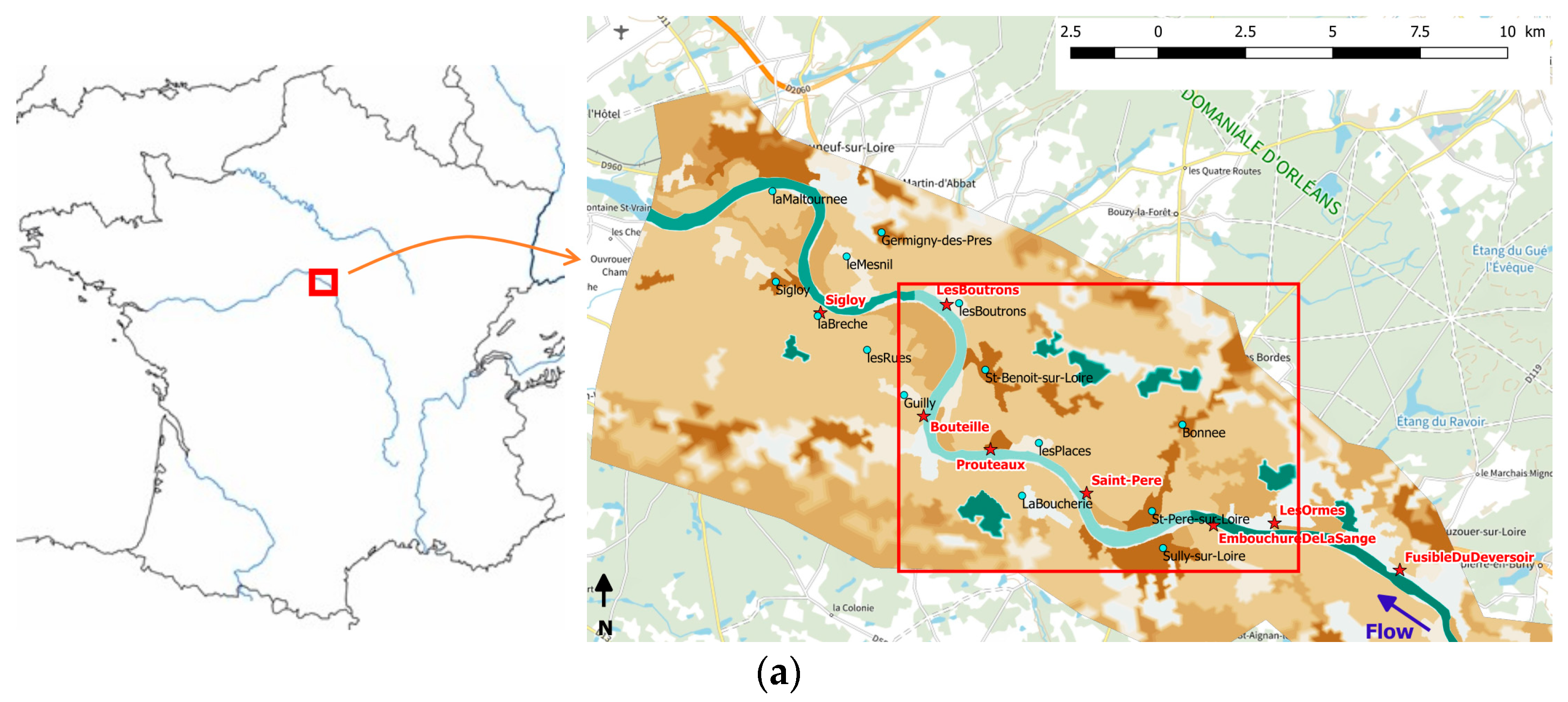
The flood hazard assessment is conducted with a 2D depth-averaged hydraulic model (i.e., shallow water equations) on a reach of the Loire river (France). The study area extends between St-Martin-sur-Ocre (upstream) and Châteauneuf-sur-Loire (downstream), which is about 50 km long (Figure 1a). Levees and longitudinal weirs were progressively built since the 19th century to protect population and assets against floods of the Loire river. In the present work, eight breaches are considered, five being located at the right side and three at the left side of the river.

2.1. Model Set Up

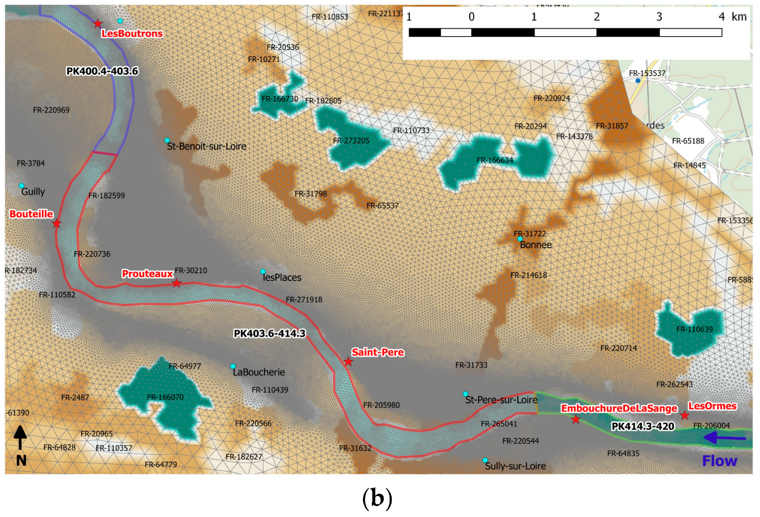
The 2D depth-averaged hydrodynamic model TELEMAC-2D, from the TELEMAC-MASCARET hydro-informatic system (www.opentelemac.org, accessed on 6 December 2021), is used to simulate free-surface flow using the finite element method on a triangular element mesh [35]. TELEMAC-2D has been widely applied for simulating flood propagation induced by levee breaching [23,36]. The mesh composed of 311,112 nodes is elaborated from break lines so that topographic singularities (e.g., roads, dikes, weirs, low walls, etc.) could be accurately described. The grid size varies from 10 to 20 m in the sectors with topographic singularities and steep slopes (e.g., main bed, levees, etc.) to more than 350 m at the edge of the valley (Figure 1b). The densely urbanized regions are numerically considered through specific friction areas. A constant flow discharge is imposed at Saint-Martin-sur-Ocre, whereas a stage-discharge relationship (measurements at gauge station at Châteauneuf-sur-Loire) is defined as a downstream boundary condition.

Figure 1. Study area: (a) domain of interest; (b) zoom area. Red stars indicate breach locations (weak points) and blue dots are points of interest in the floodplain. Colored surfaces correspond to friction coefficient areas. Range of variation of friction coefficients in the floodplain is reported in the legend.

Figure 1. Study area: (a) domain of interest; (b) zoom area. Red stars indicate breach locations (weak points) and blue dots are points of interest in the floodplain. Colored surfaces correspond to friction coefficient areas. Range of variation of friction coefficients in the floodplain is reported in the legend.

2.2. Hydrodynamic Model

TELEMAC-2D solves the following shallow water equations (Equations (1)–(3)).

$$\frac{\partial h}{\partial t}+\frac{\partial }{\partial x}\left(hu\right)+\frac{\partial }{\partial y}\left(hv\right)=0$$

(1)

$$\frac{\partial hu}{\partial t}+\frac{\partial }{\partial x}\left(huu\right)+\frac{\partial }{\partial y}\left(huv\right)=-gh\frac{\partial Z_s}{\partial x}+h{F}_x+\nabla \left(h{\nu }_e\nabla \left(u\right)\right)$$

(2)

$$\frac{\partial hv}{\partial t}+\frac{\partial }{\partial x}\left(huv\right)+\frac{\partial }{\partial y}\left(hvv\right)=-gh\frac{\partial Z_s}{\partial y}+h{F}_y+\nabla \left(h{\nu }_e\nabla \left(v\right)\right)$$

(3)

where $x$ and $y$ are horizontal Cartesian coordinates; $t$ is time; $u$ and $v$ are components of the depth-averaged velocity in x- and y-direction, respectively; $h$ is the water depth; ${\nu }_e$ is an effective diffusion representing depth-averaged turbulent viscosity ${\nu }_t$ and dispersion; $Z_s$ is the free surface elevation; $g$ is gravitational acceleration; $F_x$ and $F_y$ refer to the friction forces in x- and y-direction, respectively (Section 2.2.1). TELEMAC-2D has been validated for many analytic, experimental and real-world cases [37]. In this work, the finite element approach is used to solve the previous equation system. The N edge by edge scheme (NERDS) and the Positive Streamwise Invariant (PSI) distributive scheme are used for solving the advection of velocity and water depth, respectively. Wetting and drying of grid elements is considered through a correction of the free surface gradient [35].

2.2.1. Roughness Coefficient

The following component of the friction force is treated in a semi-implicit form within TELEMAC-2D [35]:

$$\{\begin{array}{c}{F}_x=-\frac{u}{2h}{C}_f\sqrt{u^2+v^2}\\ F_y=-\frac{v}{2h}{C}_f\sqrt{u^2+v^2}\end{array}$$

(4)

where $C_f$ is a dimensionless friction coefficient. Empirical formulas are used for calculating $C_f$ [38]. In the present work, the following Strickler formula is used, in which the Strickler coefficient $K_s$ is a parameter to be calibrated:

$$C_f=\frac{2g}{K_s{}^2{h}^{1/3}}$$

(5)

The model calibration is a reverse method which is used to find an “acceptable” friction coefficient leading to computed water levels close to the measured ones for a given flow discharge. In the present study, the Strickler coefficient is assumed constant in time and spatially distributed. Three events are retained from Banque HYDRO data [39] (December 2003 (3320 m³/s at Given, 17-year flood) from January 2008 (890 m³/s at Given, less than 1-year flood) and November 2008 (2320 m³/s at Given, 4-year flood) for calibration of the main river Strickler coefficients. Observation data are unavailable in the floodplain, and no significant flooding events have been recorded to date. Thus, the floodplain friction areas are identified based on the inventory of Corine Land Cover of 2018 [40]. For each area and following expert knowledge, the Strickler coefficient is taken as the mean value of an interval bounded by physical values depending on soil occupation.

2.2.2. Levee Breaches

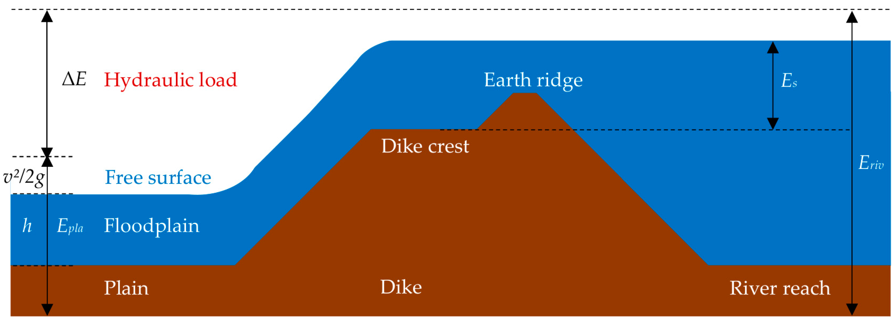
Simplified models describe the levee breaching by making assumptions on the location, initiation, development, number, and shape of the levee breach, often based on engineering experience, and knowledge of historical events [23]. In the present study, breaches are initiated at pre-defined locations (Figure 1a), identified from historical observations [41,42] and field surveys. The breach initiation occurs if the overtopping flow depth above the dike ($E_s$) reaches a threshold value and when the energy balance ($\mathsf{\Delta }E$), defined as the difference between the upstream head (channel side, $E_{riv})$ and downstream head (floodplain side, $E_{pla}$) of a weak point is high enough (Figure 2). The proposed criterion permits the taking into account of two crucial physical phenomena affecting the breach initiation: the overtopping height (the water height above the dike crest or the earth ridge) and the energy balance which can potentially prevent (or accelerate) the failure mechanisms. For instance, if the floodplain is totally inundated ($\mathsf{\Delta }E$ near to zero), no breach can form in our model. This is in agreement with safety studies performed by French public authorities (see for instance [43]).

Current state-of-the-art on the breaching of fluvial dikes due to overtopping flows shows that the breaching expansion is progressive (i.e., non-instantaneous) [44,45], following two main phases (referred to as breach formation and development, respectively). During the first phase, the breach deepening (vertical incision of the breach) is faster than the breach widening [5]. Then, when the breach bottom reaches the foundation of the dike or a non-erodible layer, only lateral widening is observed until the breach stabilizes (i.e., the fully formed breach with erosion being stopped). For the sake of simplification, we assume that the breach shape is rectangular, and its expansion follows one phase according to this linear law:

$$B\left(t\right)=k_{in}\times t,\forall t\le T_f.$$

(6)

where $t$ is time in hours (after breach initiation), $B$ is the breach width in meters at time $t$, $k_{in}$ (m/h) is the breach widening rate, assumed constant in this study, and $T_f$ is the total duration of the breach expansion.

The breach time-deepening is also described according to a linear law:

$$Z_b\left(t\right)=Z_b\left(0\right)-\frac{Z_b\left(0\right)-Z_{b,min}}{T_d}\times t,\forall t\le T_d.$$

(7)

where, $Z_b$ is the breach invert elevation at time $t$, $Z_b\left(0\right)$ is the breach invert initial elevation, $Z_{b,min}$ is the breach minimum level, and $T_d$ is the breach deepening duration. Since the breach deepening is evolving faster than the breach widening, $T_d$ is taken 10 times smaller than $T_f$.

3. Uncertainty Assessment Methodology

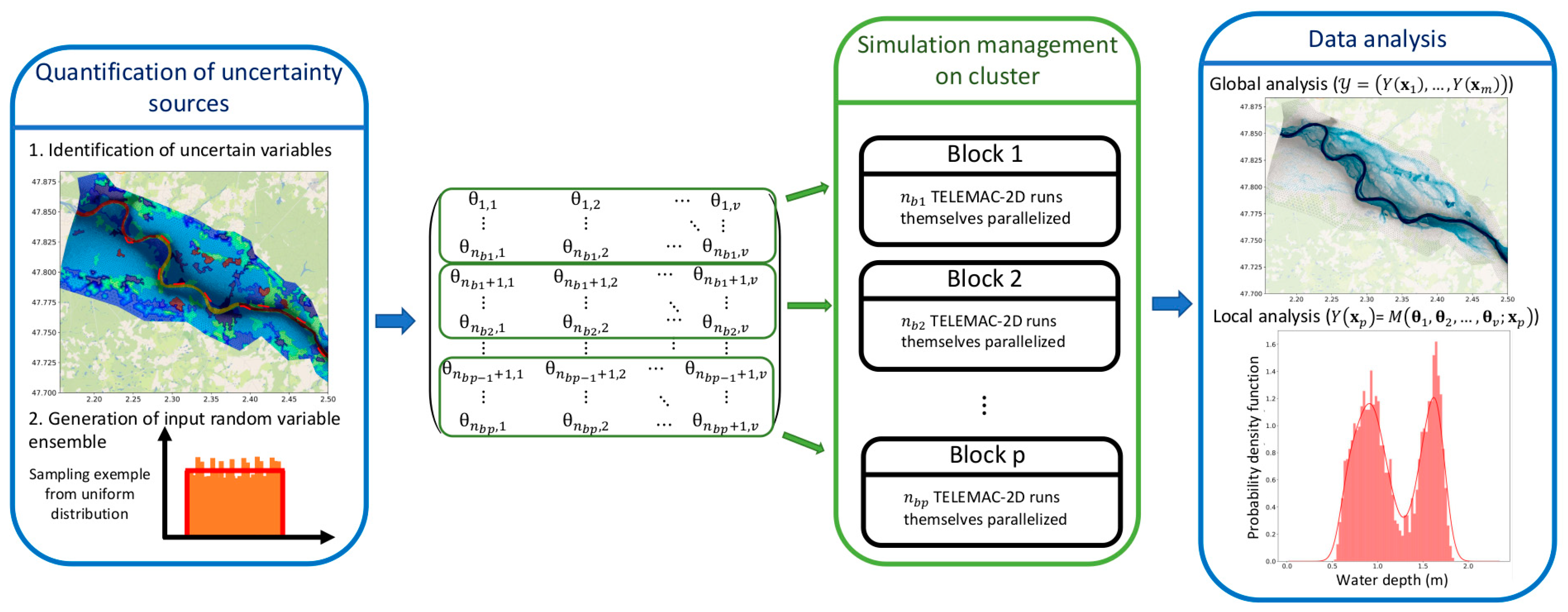
Below we describe the methodology used for assessing how the friction parameter and multiple breaches influence the flood hazard evaluation. The methodology involves three steps: (i) uncertainty quantification, (ii) uncertainty propagation, and (iii) sensitivity analysis. The Application Programing Interface (API) framework described by Goeury et al. [46] was used. The Monte Carlo approach has been implemented using MPI technology on the HPC resource for the parallel computation of all clearly separated and identifiable samples in order to be fast and compatible with industrial needs. The chart of the methodology is shown in Figure 3.

3.1. Uncertainty Quantification

3.1.1. Flood Inundation Scenarios

Extrapolated flow discharges from frequency curves of 100-, 200-, 500- and 1000-year return period scenarios, respectively, and are used as the upstream boundary condition. A real duration of four days is simulated, with a time step of 2 s, requiring one and a half hours of parallel computation with Intel-Xeon(R) Platinum 8260 processors. The quantity of interest is the flow depth at the steady state condition.

3.1.2. Uncertain Parameter Characterization

• Roughness coefficient quantification:

Following the principle of maximum entropy, a uniform distribution for the roughness coefficient is imposed. Uniform bounds in the riverbed are set to ±2.5 m^1/3s⁻¹ from the calibrated value to be compatible with the calibration accuracy of 20 to 25 cm. In the floodplain, bound values are assigned according to land cover classes as presented in

Table 1. Floodplain roughness characterization and associated probabilistic distribution.

Land Cover Class	Variation Interval (m1/3s−1)	Probability Distribution
Areas with dense urbanization	[5, 8]	Uniform
Areas with low urbanization	[8, 10]
Areas of shrubs, undergrowth	[8, 12]
Low-height agricultural areas	[10, 15]
High-height agricultural areas	[15, 20]

. A total of 280 friction areas are considered.

• Dike breach controlling coefficient quantification:

The uncertain breach parameters considered in this study are the initiation criteria and the final breach width (

Table 2. Breach parameters with associated range of variations, based on measurement uncertainty or historical analysis with geotechnical characteristics [41,42] (Failure Criterion $E_s$ and final breach width $B_f$, respectively) or defined by expert knowledge (energy balance criterion $\mathsf{\Delta }E$).

Name	$\mathbf{Dike} \mathbf{Crest} {\mathit{Z}}_{\mathit{b}}\left(0\right)$ (m NGF N)	$\mathbf{Failure} \mathbf{Criterion} {\mathit{E}}_{\mathit{s}}$ (m)	$\mathbf{Failure} \mathbf{Criterion} \mathsf{\Delta }\mathit{E}$ (m)	$\mathbf{Final} \mathbf{Breach} \mathbf{Width} {\mathit{B}}_{\mathit{f}}$ (m)	Dike Material
Fusible du déversoir	120.80	[−0.25, 0.3]	[0.3, 1.5]	[50, 850]	clay-dominated
Les ormes	119.72	[0.05, 0.6]	[0.3, 1.5]	[50, 950]	sandy-loamy
Embouchure de la Sange	118.82	[0.05, 0.6]	[0.3, 1.5]	[50, 950]	sandy-loamy
Saint-Père	116.66	[0.05, 0.6]	[0.3, 1.5]	[50, 950]	clay-dominated
Prouteaux	115.60	[−0.25, 0.3]	[0.3, 1.5]	[50, 950]	sandy-loamy
Bouteille	114.46	[−0.25, 0.3]	[0.3, 1.5]	[50, 950]	sandy-loamy
Les Boutrons	112.08	[0.05, 0.6]	[0.3, 1.5]	[50, 950]	sandy-loamy
Sigloy	111.54	[0.05, 0.6]	[0.3, 1.5]	[50, 950]	sandy-loamy

).

The breach triggering is assumed to occur at the lowest elevation point of the levee crest determined from topographic data (Lidar or survey data). Failure by overtopping (Failure Criterion $E_s$) is allowed in a certain range of variation to take into consideration the topographic measurement uncertainty (minimum permitted values (Table 2): −0.25 m and 0.05 m respectively for Lidar data and accurate topographic surveys) and geotechnical characteristics of the levee (Loire river levees typically feature a “banquette” (earth ridge) on top [47] (Figure 2) providing additional resistance to the levee characterized by a highest maximal value (0.6 m) in comparison to a dike without earth ridge (0.3 m); upper bounds in Table 2). The energy balance criterion $\mathsf{\Delta }E$ is set, following expert opinion, to [0.3, 1.5] (m). The duration of overtopping over the dike crest is not considered in this study since its quantification is subject to significant uncertainty for a relatively low potential impact [17].

The breach shape is assumed to be rectangular, characterized by its final width ($B_f$), widening rate ($k_{in}$) and final invert elevation ($Z_{b,min}$). The minimum and maximum values of the final breach width ($B_f$) interval ([50, 950] (m); Table 2) are determined from historical analysis [41] and geotechnical considerations [42]. The breach widening rate $k_{in}$ is considered constant, with values of 102 m/h and 10.2 m/h corresponding to predominantly sandy-loamy and clay-dominated structures, respectively [48,49,50]. The duration of breach widening T_f is also assumed to be deterministic and deduced from Equation (6) using $B_f$ and $k_{in}$. The breach depth is assumed to be the same as the height of the levee itself, as non-erodible layers are considered in dike foundations.

3.2. Uncertainty Propagation

To handle dynamic system behavior under parameter uncertainty, a set of sample configurations is generated using random sampling. In the sampling procedure, the parameter uncertainties are taken in a uniform distribution whose limits are defined by the minimum/maximum values of its variation range. The solver TELEMAC-2D (thereafter denoted $M$) ensures the relationship between a configuration vector of model uncertain inputs ${\mathsf{\theta }}^j=\left({\mathsf{\theta }}_{j,1},{ \mathsf{\theta }}_{j,2}\cdots {\mathsf{\theta }}_{j,v}\right)$ and the output quantity of interest $Y\left(x\right)$ whereby $Y\left(x\right)=M\left({\mathsf{\theta }}^j;x\right)$ (Figure 3). As TELEMAC-2D is a spatially discrete model, for a realization ${\mathsf{\theta }}^j$, the model output $Y$ is composed of scalar output given on a set of $m\in \mathbb{N}$ space coordinates $\left\{x_1,\dots ,x_m \right\}$ such as $Y=\left(Y_1,\dots Y_m\right)$ (with $Y_i=Y\left(x_i\right)$=$M\left({\mathsf{\theta }}^j;x_i\right)$). The full set of spatially discrete output over the complete random sampling gives a matrix of size $n\times m$ (where $n$ is the number of Monte Carlo simulations).

$$\mathcal{Y}=\left(Y_1,\dots ,Y_m\right)=\left(\begin{array}{cc}\begin{array}{cc}{y}_{1,1}& y_{1,2}\\ y_{2,1}& y_{2,2}\end{array}& \begin{array}{cc}\cdots & y_{1,m}\\ \cdots & y_{2,m}\end{array}\\ \begin{array}{cc}⋮& ⋮\\ y_{n,1}& y_{n,2}\end{array}& \begin{array}{cc}\ddots & ⋮\\ \cdots & y_{n,m}\end{array}\end{array}\right)$$

(8)

Each row of the matrix $\mathcal{Y}$ corresponds to the flow depth throughout the computational domain for a fixed upstream flow scenario of uncertain input parameter, while each column $Y_i$ in $\mathcal{Y}$ contains the values of the output variable for the full set of scenarios, at a given position $x_i$ (local analysis in Figure 3, $Y_i=Y\left(x_i\right)$=$M\left({\mathsf{\theta }}_1,{\mathsf{\theta }}_2,\dots ,{\mathsf{\theta }}_v;x_i\right)$). From matrix $\mathcal{Y}$, statistical estimators can be calculated, such as first two statistical moments (i.e., mean and variance values) or percentile of the response quantity at spatial coordinates (global analysis in Figure 3). The Monte Carlo method is robust with a convergence rate, $O\left(\sqrt{n}\right)$, that is independent of dimension, i.e., the number of factors ($v$) in the problem.

3.3. Sensitivity Analysis

The sensitivity analysis aims at quantifying the impact of uncertainty in input variables on the accuracy of the model output variables. Conventional approaches to Global Sensitivity Analysis (GSA) imply that the stochastic estimation of statistical moments [51], and indices are classically achieved with the Monte-Carlo technique [52]. To alleviate the computational burden of the Monte Carlo approach, emulators can be used to estimate sensitivity indices [53]. However, the non-linearity of local phenomena, such as dike overtopping, may affect only a small proportion of input parameter space and leads to output variability that is difficult to translate by any moment of the random variable. This can lead to uncertainty in the determination of sensitivity [54]. To obtain accurate results, a sensitivity analysis must satisfy the following requirements [55,56]: global (i.e., entire input distribution taken into consideration), model free (i.e., no assumptions on the model functional relationship to its inputs), moment independence (i.e., avoid some information loss by the use of an output variability summary) and be quantitative. In this framework, two statistical moment independence and model free GSA methods are carried out: a permutation feature importance based on a model training with machine learning and the statistical Borgonovo moment-independent sensitivity measures [56]. For the sake of clarity, in the following, the GSA methods are described in the case of scalar output such as $Y_p=Y\left(x_p\right)$=$M\left({\mathsf{\theta }}_1,{\mathsf{\theta }}_2,\dots ,{\mathsf{\theta }}_v;x_p\right)$ where $x_p$ is the location of the variable of interest.

3.3.1. Permutation Feature Importance

The permutation feature importance consists of measuring the decrease in the prediction score in a machine learning algorithm after permuting randomly an input parameter (a feature) [57]. Randomly re-ordering a parameter causes a prediction deterioration that indicates how much the model depends on the feature. If the decrease in prediction quality is small or high, the model is slightly or very sensitive to the shuffled input parameters. In this study, the prediction score is the coefficient of determination $R^2$, and random forest algorithms [57] are employed as machine learning regressors since they do not make any assumptions on the model functional relationship to its inputs.

Random forests are built by averaging the prediction of many individual decision trees. Each decision tree is fitted to a bootstrap sample created from the learning dataset (sampling matrix $\mathcal{D}=\left({\mathsf{\theta }}_1,{\mathsf{\theta }}_2,\dots ,Y_p\right)$). A decision tree is a recursive process of splitting internal nodes. To break-up a node, a collection of candidate splits is generated, and a criterion is evaluated to choose between them. For each candidate split $s=\left(k,T_{val}\right)$, the data are routed to subtrees depending on whether it exceeds the threshold value $T_{val}$ in the chosen dimension $k$ such as:

$$\{\begin{array}{c}{ℭ}_l=\left\{\left({\mathsf{\theta }}_1,{\mathsf{\theta }}_2,\dots ,Y_p\right)|{\mathsf{\theta }}_k\le T_{val}\right\}\\ {ℭ}_r=\left\{\left({\mathsf{\theta }}_1,{\mathsf{\theta }}_2,\dots ,Y_p\right)|{\mathsf{\theta }}_k>T_{val}\right\}\end{array}$$

(9)

The variance reduction method is then used to determine the optimal split at each node of the decision tree. This method is based on a calculation of the following equation:

$$\underset{s}{\max }\left({\displaystyle \sum }_{y_i\in \mathfrak{P}}\frac{{\left(y_i-\overline{y^{\mathfrak{P}}}\right)}^2}{n_p}-\frac{n_l}{n_p}{\displaystyle \sum }_{y_i\in {ℭ}_l}\frac{{\left(y_i-\overline{y^{{ℭ}_l}}\right)}^2}{n_l}-\frac{n_r}{n_p}{\displaystyle \sum }_{y_i\in {ℭ}_r}\frac{{\left(y_i-\overline{y^{{ℭ}_r}}\right)}^2}{n_r}\right)$$

(10)

where $\mathfrak{P}$ denotes the parent node containing $n_p$ training samples, ${ℭ}_l$, ${ℭ}_r$ are respectively the left and right child node subtrees containing respectively $n_l$, $n_r$ data, and $\overline{y^{\mathfrak{x}}}$ is the mean value of output values in the node $\mathfrak{x}\in \left\{\mathfrak{P}, {ℭ}_l,{ℭ}_r\right\}$.

The terminal nodes of a tree, also called leaf nodes, provide the final prediction by averaging the output of training samples within the corresponding leaf node. The methodology described here before was performed based on an open-source library for Machine Learning named “scikit-learn” [58].

3.3.2. Borgonovo Sensitivity Analysis

Moment-independent sensitivity measures overcome the output variability summary associated with the interpretation of variance-based measures. In this framework, a sensitivity measure based on the shift between the output distribution and the same distribution conditionally to a parameter was proposed [56] and reads as:

$${\delta }_i=\frac{1}{2}\left[{\displaystyle \int }{\pi }_{{\mathsf{\Theta }}_i}\left({\mathsf{\theta }}_i\right)\left[{\displaystyle \int }\left|{\pi }_Y\left(y\right)-{\pi }_{Y|{\mathsf{\Theta }}_i}\left(y\right)\right|dy\right]{d\mathsf{\theta }}_i\right]$$

(11)

However, based on the entire distribution, the Borgonovo sensitivity analysis can become unsuitable when the computational cost of each run of the model is non negligible or the number of model inputs is large. Thus, a sample-based estimation was proposed to handle this issue [59]. In the present work, this Borgonovo sensitivity analysis was carried out based on an open-source library for performing the sensitivity analyses “SALib” [60].

4. Results

Separated and identifiable Monte Carlo simulations were performed based on the MPI parallel computing technology for launching and managing the TELEMAC-2D solver computations (Figure 3). A sample set of size n = 3000 is set for the uncertainty propagation. This number was determined based on a convergence study carried at some control points (see Section 4.2). It was also checked in terms of the robustness of sensitivity estimates through asymptotic confidence intervals (Table 4). The obtained results are analyzed twofold: on one hand, a global statistical analysis on the whole domain is performed. On the other hand, the effect of the variability of the random inputs is assessed at some specific points (selected around a populated area, for example, as reported in Figure 1).

4.1. Global Statistical Analysis

4.1.1. Uncertainty Propagation

Figure 4 shows the probabilistic flood hazard maps of the 90th percentile water depths. These results could be of importance for flood management by identifying water surface elevations and lateral flood extents for each flood event. As expected, the 90th percentile water depth level increases with the rise in the flood return period. To better analyze the lateral flood extents, the 90th percentile scalar flow velocity calculated for different flood events of different return periods is also computed and presented in Figure 5.

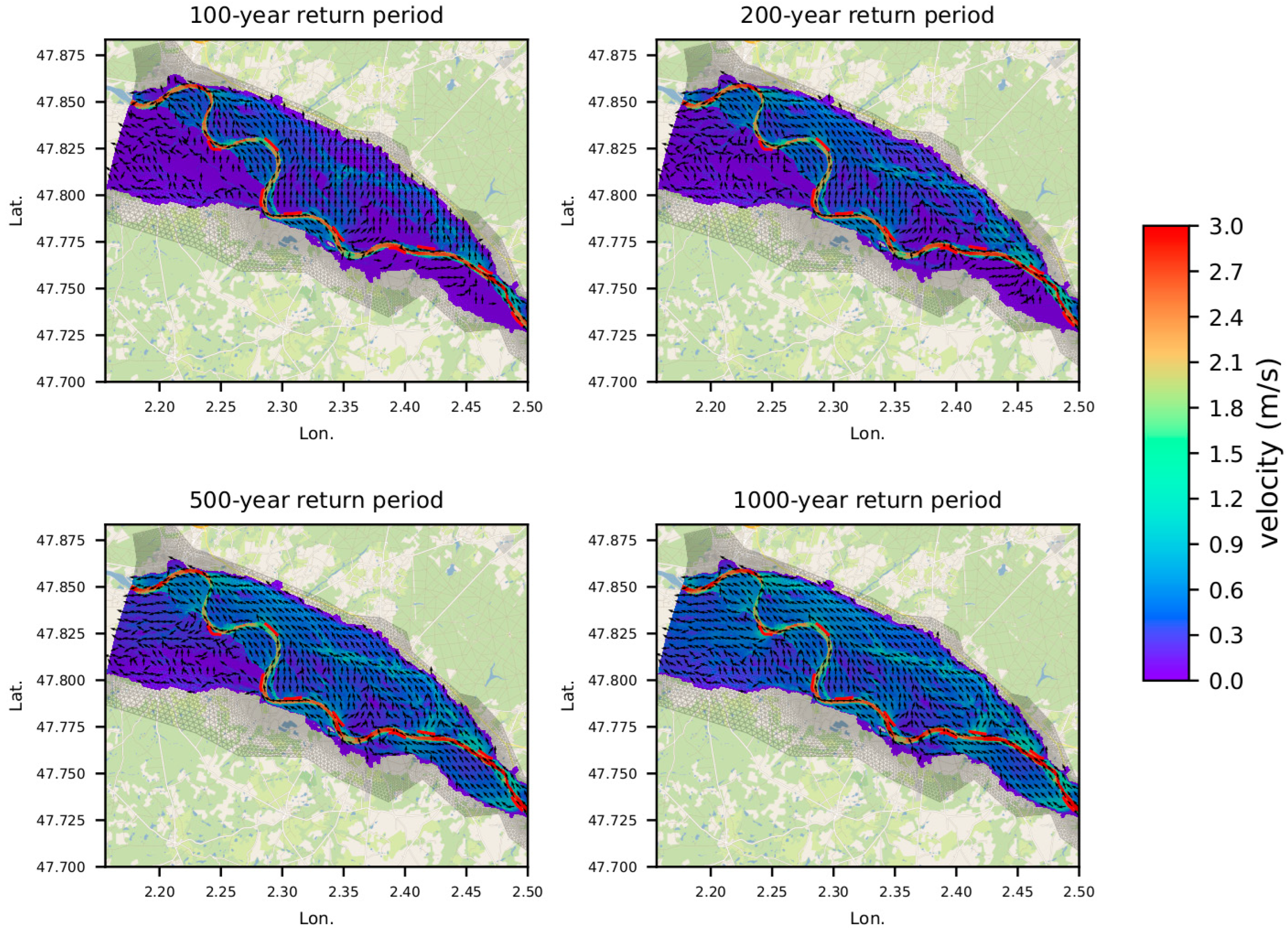
It can be noticed that not all dike breaches are formed for the different scenarios. The water elevation in the right floodplain is directly influenced by the Fusible du déversoir, Saint-Père and Les Boutrons levee breaches (Figure 1) which occur from the 100-year return period flood event. On the other hand, the significative rise in water elevation in the left floodplain occurs at high flood event scenarios with Embouchure De La Sange and Sigloy levee breaches (Figure 1). As a result, in terms of flood mitigation, it is imperative that hazards related to levee systems are thoroughly evaluated.

4.1.2. Sensitivity Analysis

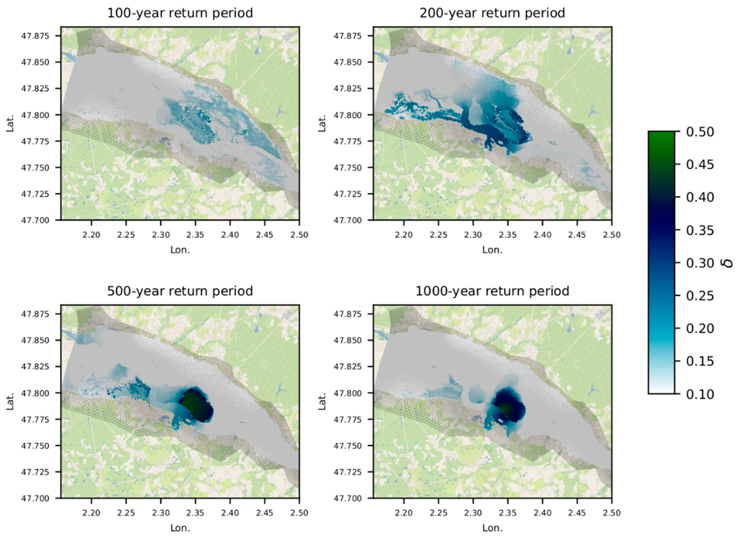
For a given flood scenario, the breach width can significantly affect the water heights in the floodplain since it is a parameter influencing the breach outflow hydrographs [15]. Figure 6 shows the computation of the Borgonovo index to evaluate the influence of a breach width on the water depth. Particularly, a value close to 0 and, conversely, 1 means that the output is, respectively, independent or highly dependent on the variable of interest. Figure 6 highlights the spatial influence scale and intensity of the Saint-Père breach width uncertain variable on the water depth. The intensity of the parameter influence increases with increasing flood scenarios’ discharge. This increase is accompanied by a more localized spatial effect, emphasizing the need for local flood analysis to better understand the conditions under which flood mitigation is most likely to occur, thereby helping to make communities more resilient to flooding [61].

4.2. Local Statistical Analysis

4.2.1. Uncertainty Propagation

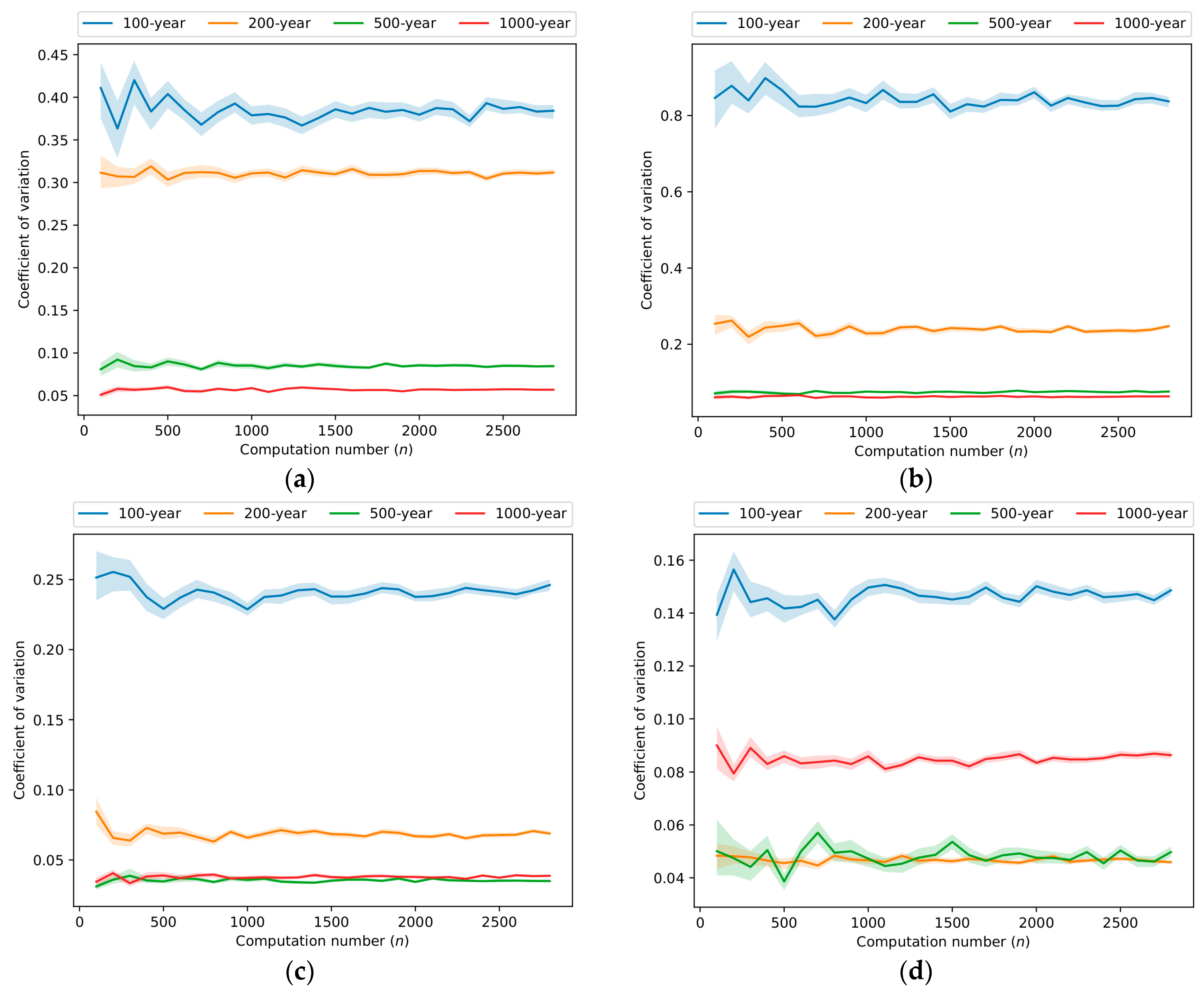
A statistical analysis of flow depth values at specific locations yields a valuable tool for understanding the flooding patterns. When applying a sampling-based statistical analysis, the estimators are not computed exactly but rather approximated from the available samples. To assess the robustness and convergence of such estimates, the convergence rates of the statistical coefficient of variation (ratio of the standard deviation to the mean) and its 90% confidence interval obtained by the bootstrap method are evaluated as the sample size $n$ increases for the points of interest (see locations on Figure 1). As illustrated in Figure 7, the number of samples needed to reach stable statistical estimates can vary from one discharge to another. However, from a sample size of 2500, the statistical estimators are stabilized for all the points of interest of this study. Thus, the number of 3000 model evaluations considered in this study is satisfactory to obtain reliable results. The robustness of the statistical coefficient of variation is analysed through confidence intervals. They are estimated from 100 bootstrap samples. As shown in

Table 3. 90% confidence intervals of the coefficient of variation obtained from the Monte Carlo sample set of 3000 computations for 100, 200, 500 and 1000-year return period flood scenarios at some control points.

Control Points	Sully-Sur-Loire	Les Places	Les Boutrons	Le Mesnil
100-years flood scenario	$\left[0.375, 0.391\right]$	$\left[0.821 , 0.849\right]$	$\left[0.242 , 0.25\right]$	$\left[0.147, 0.150\right]$
200-years flood scenario	$\left[0.309, 0.315\right]$	$\left[0.242 , 0.252\right]$	$\left[0.0676 , 0.0704\right]$	$\left[0.0452 , 0.0465\right]$
500-years flood scenario	$\left[0.0834, 0.0865\right]$	$\left[0.0747 , 0.779\right]$	$\left[0.0342 , 0.036\right]$	$\left[0.0479 , 0.0518\right]$
1000-years flood scenario	$\left[0.0562, 0.0579\right]$	$\left[0.0623 , 0.0641\right]$	$\left[0.0379 , 0.0394\right]$	$\left[0.0851 , 0.0877\right]$

, the bounds of the confidence intervals are relatively close and demonstrate the capacity of Monte Carlo sampling to produce accurate estimates for the points of interest of this study.

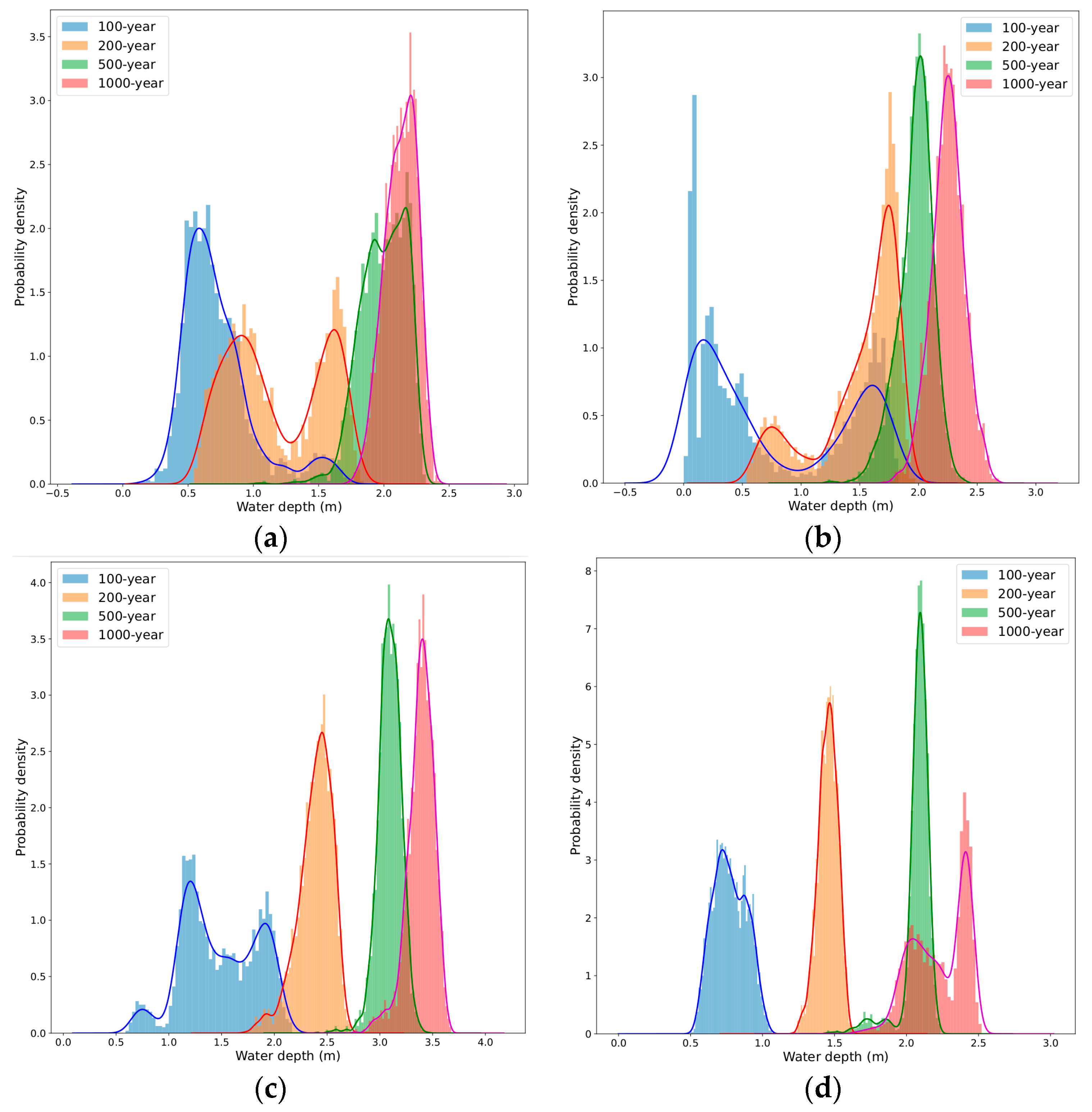
Figure 8 displays how the model parameter uncertainties (roughness coefficients and levee breach characteristics) affect the water depth at selected locations for given flood scenarios. The spreading of the water depth distribution is more significant for low flood scenarios (100-year return period) and diminishes with the rise in the flood discharge. This demonstrate that high flood scenarios are less sensitive to the selected uncertain parameters. The results highlight the complexity of the flow with non-symmetric (non-Gaussian) water level distributions. Some water level distributions show multiple peaks in the PDF, especially for low flood scenarios. These multimodal distributions indicate that the control point sample can have several patterns of response, suggesting that the flooding patterns can drastically change, starting from a given combination of the uncertain inputs.

4.2.2. Sensitivity Analysis

Table 4. Sensitivity analysis at Les Places control point for 100, 200, 500 and 1000-year return period flood events: Borgonovo indices and permutation feature importance with their corresponding asymptotic confidence intervals, typically with a confidence level of 90%. PK and FR indicates, respectively, the friction coefficients for the riverbed and the floodplain (as reported in Figure 1).

Methods	Borgonovo Indices	Permutation Importance
100-years flood scenario	Saint-Père overtopping level: 0.22 ± 0.011	Fusible du déversoir overtopping level: 0.73 ± 0.028
	Fusible du déversoir overtopping level: 0.20 ± 0.011	Saint-Père overtopping level: 0.72 ± 0.024
	PK403-414: 0.12 ± 7.2 × 10−3	PK403-414: 0.33 ± 0.02
	Saint-Père breach width: 0.10 ± 4.2 × 10−3	PK414-420: 0.099 ± 6 × 10−3
	Fusible du déversoir breach width: 0.091 ± 3.9 × 10−3	Saint-Père breach width: 0.018 ± 1.4 × 10−3
	FR-64977: 0.09 ± 4.3 × 10−3	FR-64977: 0.0083 ± 6.9 × 10−4
200-years flood scenario	Saint-Père breach width: 0.22 ± 9.9 × 10−3	Saint-Père overtopping level: 0.91 ± 0.039
	Saint-Père overtopping level: 0.21 ± 0.011	PK403-414: 0.57 ± 0.028
	PK403-414: 0.13 ± 8.29 × 10−3	Saint-Père breach width: 0.24 ± 9.7 × 10−3
	Prouteaux overtopping level: 0.097 ± 6 × 10−3	FR-64977: 0.081 ± 5.6 × 10−3
	FR-64977: 0.083 ± 7.8 × 10−3	Fusible du déversoir breach width: 0.045 ± 4 × 10−3
	Fusible du déversoir breach width: 0.078 ± 7 × 10−3	Prouteaux overtopping level: 0.01 ± 1 × 10−3
500-years flood scenario	Saint-Père breach width: 0.32 ± 0.011	Saint-Père breach width: 1.12 ± 0.042
	FR-65537: 0.1 ± 0.01	FR-65537: 0.30 ± 0.018
	Les Ormes overtopping level: 0.085 ± 7.02 × 10−3	Prouteaux overtopping level: 0.14 ± 0.011
	Prouteaux overtopping level: 0.081 ± 9.1 × 10−3	Les Ormes overtopping level: 0.12 ± 0.01
	PK403-414: 0.071 ± 7.65 × 10−3	PK403-414: 0.048 ± 4.4 × 10−3
	Les Ormes breach width: 0.058 ± 9 × 10−3	Prouteaux breach width: 0.047 ± 5.8 × 10−3
1000-years flood scenario	FR-65537: 0.22 ± 0.014	FR-65537: 0.68 ± 0.028
	Saint-Père breach width: 0.19 ± 9.84 × 10−3	Saint-Père breach width: 0.63 ± 0.023
	Prouteaux overtopping level: 0.10 ± 0.012	Prouteaux overtopping level: 0.23 ± 0.011
	PK403-414: 0.098 ± 0.011	PK403-414: 0.14 ± 6.2 × 10−3
	Prouteaux breach width: 0.062 ± 9.55 × 10−3	Prouteaux breach width: 0.10 ± 8.4 × 10−3
	Les Ormes breach width: 0.054 ± 7.1 × 10−3	Les Ormes breach width: 0.08 ± 8.9 × 10−3

summarizes the sensitivity results at Les Places control point. The robustness of the sensitivity indices is analysed through confidence intervals. They are obtained asymptotically from the standard deviation estimated with 100 bootstrap samples. As mentioned in Section 3.3, random forest regressors were used to compute the permutation feature importance score. Here, for each point of interest and flood scenario, a collection of possible regressors, ordered by number and depth of decision trees, is provided and an optimum is chosen in terms of learning and prediction score (coefficient of determination $R^2$). The train and test subsets are randomly obtained after splitting the Monte Carlo sample set in the percent proportion of 80 and 20, respectively. Thus, for each point of interest and flood scenario, an optimum Random Forest regressor with a coefficient of determination $R^2$ higher than 0.98 and 0.75 for learning and predictive score is obtained and considered satisfactory in a study framework, respectively.

The sensitivity analysis methods tested in this work lead to a similar ranking of the importance of the uncertain parameters. This statement, in contrast to the work presented in [54], confirms the requirement for sensitivity analysis (global, model free, moment independence and be quantitative) to produce accurate results. Of all the uncertain input parameters, only several (levee breach parameters and roughness coefficient close to the point of interest) are identified as playing a major role in the accuracy of the water level at the relevant control point.

The physical interpretation of the sensitivity results allows a clearer understanding of the flood hazard. The concomitance of the Saint-Père and Fusible du déversoir breaches could be at the origin of the bimodal behavior in the PDF observed for the 100-year return period flood scenario. In fact, the overtopping variables $E_s$ and $\mathsf{\Delta }E$ for the initiation of these two breaches appear to be, with the same relative weight, the most important factors. The increase in flow rate is accompanied by a major impact of the Saint-Père breach width, leading progressively to a single peak in the water depth distribution. These results are consistent with the physics of flow. In the case of a low flood event (100-year return period flood), overtopping level and bed roughness are of primary importance since they directly influence the initiation of dike breaching. For higher return period floods, overtopping always occurs (whatever the overtopping level and bed friction parameters) and the water level at the point of interest is directly influenced by the breach discharge (which depends on the breach width) and the local floodplain roughness (FR-65537). Moreover, the control point is located between two potential dike failure locations (the Saint-Père and Prouteaux breaches). However, the dike failure at Saint-Père, which is located upstream from the control point, appears as the most influential factor. The Fusible du déversoir breach acts as a fuse plug dike clipping the flood between the 100 and 200-year return period floods. Then, other breaches (Les Ormes and Prouteaux) form along the Loire river, which increase the water depth at the control point. This finding leads to the conclusion that in a hydraulic study of inundations induced by multiple breaches, the breach development chronology affects probabilities of the formation of downstream breaches, and thus the flood hazard [26], especially for flooding events close to the design conditions for river dikes. It can be noticed that the water level at the control point is also controlled by friction coefficients in its neighboring zone. As expected, the riverbed and floodplain friction coefficients (identified as “PK403-414” and “FR-65537”) also have an impact on the water level at low and high flow, respectively.

5. Discussion

In this study, the effect of the uncertainty resulting from the stochastic processes of dike breaches and roughness coefficients on water level calculations for extreme flood events was investigated. The analysis presented in this work can be carried out on other quantities of interest, such as scalar flow velocity ($\left|v\right|$), flood hazard index [28], total force and/or total depth indicators [9]. Based on the Froude number, the last indicator has been investigated. Since the Froude number has a limited impact in the computational domain, no significative difference is observed with the water depth analysis presented in the previous section. As for quantity of interest, the methodology described in this paper can be applied for other uncertain parameters. In a steady state condition, integrating breach development times has no major impact on the numerical results in comparison to instantaneous and complete breaches computation. However, in the case of unsteady flow, this parameter variability in interaction to other ones (e.g., breach width) can significantly affect the dike failure probability [26]. In that case, it also could be interesting to test the influence of parametric laws for the breach expansion [36].

A major issue arising from the methodology presented in the current study concerns the optimization of the number of computational runs needed for sufficient results in the uncertainty analysis. The Monte Carlo technique, while generic and robust, is also computationally expensive due to its low convergence rate. Ways to reduce the computational cost typically require the replacement of the pure random sampling that forms the backbone of the Monte Carlo method by alternative sampling methods such as the optimized Latin Hypercube Sampling (LHS) approaches [62].

To handle the high-dimensional uncertain input space problem, special attention was paid to proposing a relevant sensitivity analysis to produce accurate and robust results. Thus, two moment independence and model free GSA methods have been investigated. Although the ranking is similar between the two methods tested, the permutation importance based on random forest provides a better distinction between influential and non-influential parameters. However, this statement needs to be completed by investigating the effect of the computation number on the sensitivity analysis methods. This was not studied here and will be the topic of a future study.

Despite the fact that the permutation importance method has informal and strong connections with Sobol’ sensitivity theory [63], the method is considered in the paper as a moment independence and model-free GSA method. Indeed, the permutation importance method based on the random forest algorithm is assumed to be model-free since it does not make any assumptions on the model functional relationship to its inputs. In addition, no explicit statistical moment of the output variable is decomposed by the machine learning approach, which is why it is designed as the moment independence method.

6. Conclusions and Perspectives

The effect of uncertainty resulting from the stochastic processes of multiple dike breaches and roughness coefficients on water level calculation was investigated numerically for different extreme flood scenarios on a reach of the Loire river. To address the uncertainty analysis in high dimensional spaces, a 2D depth-averaged hydraulic model was run in a Monte Carlo framework. Inundation hazard maps for different flood scenarios highlighted the important impact of the breach development chronology. To overcome the non-linearity difficulty of local phenomena, such as the overtopping of a dike, moment independence and model free sensitivity analysis methods were carried out to assess the factors influencing the flow depth and flood extent. The spatial analysis of vulnerability area induced by levee breaching showed that, with increasing flood discharge, the rise of variable influence intensity is accompanied by a more localized spatial effect. This argues for local flood analysis to allow a sound understanding of the flood hazard for these scenarios. The physical interpretation, highlighted by the Global Sensitivity Analysis (GSA), emphasized that interactions between breach parameters and roughness coefficients play a significant role in the water level uncertainty.

The quantification of uncertainty in roughness coefficients was done following expert knowledge, but potentially available sources of information (e.g., in situ and remote sensing data) can be employed. The effect of other uncertain breach parameters (e.g., overtopping duration, widening stages and associated kinetics, breaching duration, breach shape) and other causes of breaching (e.g., piping) can be also considered in future works. Uncertainty also arises from boundary conditions (state-discharge and discharge frequency curves), hydraulic model parameterization (roughness coefficient, behavior of hydraulic and protection structures) and geometric description (bathymetric and topographic data). Even if difficult, these uncertainties should also be considered from both modelers and decision-makers to propose an adapted strategy for hazard mitigation. Handling uncertainty in hydraulic study is central to sustainable and successful flood risk management [64] involving public safety and economic damage. Communicating uncertainty analysis to decision makers in order to construct a consensus for a flood hazard management process is a new challenge to overcome [65].

References

- European Environment Agency. Available online: https://www.eea.europa.eu/publications/economic-losses-and-fatalities-from/economic-losses-and-fatalities-from (accessed on 10 February 2022).
- Freer, J.; Beven, K.J.; Neal, J.; Schumann, G.; Hall, J.; Bates, P. Flood Risk and Uncertainty. In Risk and Uncertainty Assessment for Natural Hazards; Cambridge University Press: Cambridge, UK, 2013; pp. 190–233. [Google Scholar] [CrossRef] [Green Version]
- Ghazali, D.A.; Guericolas, M.; Thys, F.; Sarasin, F.; Arcos González, P.; Casalino, E. Climate Change Impacts on Disaster and Emergency Medicine Focusing on Mitigation Disruptive Effects: An International Perspective. Int. J. Environ. Res. Public Health 2018, 15, 1379. [Google Scholar] [CrossRef] [Green Version]
- Tabari, H. Climate change impact on flood and extreme precipitation increases with water availability. Sci. Rep. 2020, 10, 13768. [Google Scholar] [CrossRef]
- Rifai, I.; Erpicum, S.; Archambeau, P.; Violeau, D.; Pirotton, M.; El kadi Abderrezzak, K.; Dewals, B. Overtopping induced failure of non-cohesive homogenous dikes. Water Resour. Res. 2017, 53, 3373–3386. [Google Scholar] [CrossRef] [Green Version]
- Özer, I.E.; van Damme, M.; Jonkman, S.N. Towards an International Levee Performance Database (ILPD) and Its Use for Macro-Scale Analysis of Levee Breaches and Failures. Water 2020, 12, 119. [Google Scholar] [CrossRef] [Green Version]
- Akhter, F.; Mazzoleni, M.; Brandimarte, L. Analysis of 220 Years of Floodplain Population Dynamics in the US at Different Spatial Scales. Water 2021, 13, 141. [Google Scholar] [CrossRef]
- FEMA (Federal Emergency Management Agency). Guidance for Flood Risk Analysis and Mapping, Flood Risk Assessments; FEMA: Washington, DC, USA, 2020.
- Ferrari, A.; Dazzi, S.; Vacondio, R.; Mignosa, P. Enhancing the resilience to flooding induced by levee breaches in lowland areas: A methodology based on numerical modelling. Nat. Hazards Earth Syst. Sci. 2020, 20, 59–72. [Google Scholar] [CrossRef] [Green Version]
- Pappenberger, F.; Beven, K.J.; Horritt, M.; Blazkova, S. Uncertainty in the calibration of effective roughness parameters in HEC-RAS using inundation and downstream level observations. J. Hydrol. 2005, 302, 46–69. [Google Scholar] [CrossRef]
- Aronica, G.T.; Franza, F.; Bates, P.D.; Neal, J.C. Probabilistic evaluation of flood hazard in urban areas using monte carlo simulation. Hydrol. Process. 2012, 26, 3962–3972. [Google Scholar] [CrossRef]
- Abily, M.; Delestre, O.; Bertrand, N.; Duluc, C.-M.; Gourbesville, P. High-resolution Modelling With Bi-dimensional Shallow Water Equations Based Codes –High-Resolution Topographic Data Use for Flood Hazard Assessment Over Urban and Industrial Environments. Procedia Eng. 2016, 154, 853–860. [Google Scholar] [CrossRef]
- Vorogushyn, S.; Merz, B.; Lindenschmidt, K.-E.; Apel, H. A new methodology for flood hazard assessment considering dike breaches. Water Resour. Res. 2010, 46, W08541. [Google Scholar] [CrossRef] [Green Version]
- Mazzoleni, M.; Bacchi, B.; Barontini, S.; Di Baldassarre, G.; Pilotti, M.; Ranzi, R. Flooding hazard mapping in floodplain areas affected by piping breaches in the Po River, Italy. J. Hydrol. Eng. 2014, 19, 717–731. [Google Scholar] [CrossRef]
- Mazzoleni, M.; Dottori, F.; Brandimarte, L.; Tekle, S.; Martina, M.L.V. Effects of levee cover strength on flood mapping in the case of levee breach due to overtopping. Hydrol. Sci. J. 2017, 62, 892–910. [Google Scholar] [CrossRef]
- Ciullo, A.; de Bruijn, K.M.; Kwakkel, J.H.; Klijn, F. Accounting for the uncertain effects of hydraulic interactions in optimising embankments heights: Proof of principle for the IJssel River. J. Flood Risk Manag. 2019, 12, e12532. [Google Scholar] [CrossRef]
- Curran, A.; De Bruijn, K.M.; Kok, M. Influence of water level duration on dike breach triggering, focusing on system behaviour hazard analyses in lowland rivers. Georisk Assess. Manag. Risk Eng. Syst. Geohazards 2020, 14, 26–40. [Google Scholar] [CrossRef]
- Legleiter, C.J.; Kyriakidis, P.C.; McDonald, R.R.; Nelson, J.M. Effects of uncertain topographic input data ontwo-dimensional flow modeling in a gravel-bed river. Water Resour. Res. 2011, 47, W03518. [Google Scholar] [CrossRef]
- Domeneghetti, A.; Castellarin, A.; Brath, A. Assessing rating-curve uncertainty and its effects on hydraulic model calibration. Hydrol. Earth Syst. Sci. 2012, 16, 1191–1202. [Google Scholar] [CrossRef] [Green Version]
- Willis, T.; Wright, N.; Sleigh, A. Systematic analysis of uncertainty in 2D flood inundation models. Environ. Model. Softw. 2019, 122, 104520. [Google Scholar] [CrossRef]
- ASCE/EWRI Task Committee on Dam/Levee Breaching. Earthen Embankment Breaching. J. Hydraul. Eng. 2011, 137, 1549–1564. [Google Scholar] [CrossRef]
- Dazzi, S.; Vacondio, R.; Mignosa, P. Integration of a levee breach erosion model in a GPU-accelerated 2D shallow water equations code. Water Resour. Res. 2019, 55, 682–702. [Google Scholar] [CrossRef]
- Tadesse, Y.B.; Fröhle, P. Modelling of Flood Inundation due to Levee Breaches: Sensitivity of Flood Inundation against Breach Process Parameters. Water 2020, 12, 3566. [Google Scholar] [CrossRef]
- Wahl, T.L. Uncertainty of predictions of embankment dam breach parameters. J. Hydraul. Eng. 2004, 130, 389–397. [Google Scholar] [CrossRef]
- Apel, H.; Merz, B.; Thieken, A.H. Influence of dike breaches on flood frequency estimation. Comput. Geosci. 2009, 35, 907–923. [Google Scholar] [CrossRef] [Green Version]
- Vorogushyn, S.; Apel, H.; Merz, B. The impact of the uncertainty of dike breach development time on flood hazard. Phys. Chem. Earth Parts A/B/C 2011, 36, 319–323. [Google Scholar] [CrossRef] [Green Version]
- Pheulpin, L.; Bertrand, N.; Bacchi, V. Uncertainty quantification and global sensitivity analysis with dependent inputs parameters: Application to a basic 2D-hydraulic model. LHB 2022, 108, 1. [Google Scholar] [CrossRef]
- D’Oria, M.; Maranzoni, A.; Mazzoleni, M. Probabilistic assessment of flood hazard due to levee breaches using fragility functions. Water Resour. Res. 2019, 55, 8740–8764. [Google Scholar] [CrossRef]
- Morales-Hernandez, M.; Petaccia, G.; Brufau, P.; Garcıa-Navarro, P. Conservative 1D–2D coupled numerical strategies applied to river flooding: The Tiber (Rome). Appl. Math. Model. 2016, 40, 2087–2105. [Google Scholar] [CrossRef]
- Teng, J.; Jakeman, A.J.; Vaze, J.; Croke, B.F.W.; Dutta, D.; Kim, S. Flood inundation modelling: A review of methods, recent advances and uncertainty analysis. Environ. Model. Soft. 2017, 90, 201–216. [Google Scholar] [CrossRef]
- García-Navarro, P.; Murillo, J.; Fernández-Pato, J.; Echeverribar, I.; Morales-Hernández, M. The shallow water equations and their application to realistic cases. Environ. Fluid. Mech. 2019, 19, 1235–1252. [Google Scholar] [CrossRef] [Green Version]
- Pheulpin, L.; Bacchi, V.; Bertrand, N. Comparison Between Two Hydraulic Models (1D and 2D) of the Garonne River: Application to Uncertainty Propagations and Sensitivity Analyses of Levee Breach Parameters. In Advances in Hydroinformatics; Gourbesville, P., Caignaert, G., Eds.; Springer: Singapore, 2020. [Google Scholar] [CrossRef]
- Maranzoni, A.; D’Oria, M.; Mazzoleni, M. Probabilistic flood hazard mapping considering multiple levee breaches. Water Resour. Res. 2022, 58, e2021WR030874. [Google Scholar] [CrossRef]
- Huthoff, F.; Remo, J.; Pinter, N. Hydrodynamic levee-breach and inundation modelling. J. Flood Risk Manage. 2015, 8, 2–18. [Google Scholar] [CrossRef]
- Hervouet, J.-M. Hydrodynamics of Free Surface Flows: Modelling With the Finite Element Method; John Wiley & Sons: Chichester, UK, 2007. [Google Scholar]
- Kheloui, L.; El Kadi Abderrezzak, K.; Bourban, S. Simplified physically-based modelling of overtopping induced levee breaching with TELEMAC-2D. In Proceedings of the TELEMAC-MASCARET User Conference, Antwerp, Belgium, 14–15 October 2021. [Google Scholar]
- Hervouet, J.-M.; Bates, P. The TELEMAC modelling system Special issue. Hydrol. Process. 2000, 14, 2207–2208. [Google Scholar] [CrossRef]
- Morvan, H.; Knight, D.; Wright, N.; Tang, X.; Crossley, A. The concept of roughness in fluvial hydraulics and its formulation in 1D, 2D and 3D numerical simulation models. J. Hydraul. Res. 2008, 46, 191–208. [Google Scholar] [CrossRef]
- HydroPortail. Available online: http://www.hydro.eaufrance.fr (accessed on 4 April 2021).
- Copernicus Land Monitoring Service. Available online: https://land.copernicus.eu/pan-european/corine-land-cover (accessed on 28 March 2021).
- Maurin, J.; Boulay, A.; Piney, S.; Le Barbu, E.; Tourment, R. Les brèches des levées de la Loire: Brèche de Jargeau 1856. In Proceedings of the Congrès SHF Événements Extrêmes Fluviaux et Maritimes, Paris, France, 1–2 February 2012. [Google Scholar]
- DREAL. Études de Dangers des Digues de Classe A de la Loire Moyenne Éléments de Synthèse Relatifs à L’analyse des Brèches Historiques; DREAL: Blois, France, 2012. [Google Scholar]
- Cuvillier, L.; Bontemps, A.; Manceau, N.; Patouillard, S. Connaissance et prévention du risque inondation sur les vals d’Orléans–Apport de la modélisation hydraulique 2D à une échelle globale. In Proceedings of the Hydraulique des Barrage et des Digues, Chambéry, France, 29–30 November 2017. [Google Scholar] [CrossRef]
- Rifai, I.; El Kadi Abderrezzak, K.; Erpicum, S.; Archambeau, P.; Violeau, D.; Pirotton, M.; Dewals, B. Floodplain backwater effect on overtopping induced fluvial dike failure. Water Resour. Res. 2018, 54, 9060–9073. [Google Scholar] [CrossRef]
- Wu, W.; Li, H. A simplified physically-based model for coastal dike and barrier breaching by overtopping flow and waves. Coast. Eng. 2017, 130, 1–13. [Google Scholar] [CrossRef]
- Goeury, C.; Audouin, Y.; Zaoui, F. Interoperability and computational framework for simulating open channel hydraulics: Application to sensitivity analysis and calibration of Gironde estuary model. Environ. Model. Softw. 2022, 148, 105243. [Google Scholar] [CrossRef]
- Auriau, L.; Mériaux, P.; Royet, P.; Tourment, R.; Lacombe, S.; Maurin, J.; Boulay, A. FloodProBE Project WP 3: Reliability of Urban Flood Defences. Guidebook for Using Helicopter-Borne Lidar to Contribute to Levee Assessment–Experiment on “Val d’Orléans” Pilot Site, IRSTEA. 2012. Available online: https://hal.inrae.fr/hal-02600693 (accessed on 20 October 2022).
- Zomorodi, K. Empirical Equations for Levee Breach Parameters Based on Reliable International Data. In Proceedings of the Dam Safety 2020, Association of State Dam Safety Officials, Virtual Conference, Online, 21–25 September 2020. [Google Scholar]
- Resio, D.T.; Boc, S.J.; Maynord, S.; Ward, D.; Abraham, D.; Dudeck, D.; Welsh, B. Development and Demonstration of Rapid Repair of Levee Breaching Technology; Department of Homeland Security: Vicksburg, MS, USA, 2009.
- U.S. Bureau of Reclamation (USBR). Downstream Hazard Classification Guidelines, ACER Technical Memorandum No. 11; U.S. Bureau of Reclamation, U.S. Department of the Interior: Denver, CO, USA, 1988.
- Sobol’, I.M. Global sensitivity indices for nonlinear mathematical models and their monte carlo estimates. Math. Comput. Simul. 2001, 55, 271–280. [Google Scholar] [CrossRef]
- Saltelli, A. Making best use of model evaluations to compute sensitivity indices. Comput. Phys. Comm. 2002, 145, 280–297. [Google Scholar] [CrossRef]
- Sudret, B. Global sensitivity analysis using polynomial chaos expansions. Reliab. Eng. Syst. Saf. 2008, 93, 964–979. [Google Scholar] [CrossRef]
- Pappenberger, F.; Beven, K.J.; Ratto, M.; Matgen, P. Multi-method global sensitivity analysis of flood inundation models. Adv. Water Resour. 2008, 31, 1–14. [Google Scholar] [CrossRef]
- Saltelli, A. Sensitivity analysis for importance assessment. Risk Anal. 2002, 22, 579–590. [Google Scholar] [CrossRef]
- Borgonovo, E. A new uncertainty importance measure. Reliab. Eng. Syst. Saf. 2007, 92, 771–784. [Google Scholar] [CrossRef]
- Breiman, L. Random Forests. Mach. Learn. 2021, 45, 5–32. [Google Scholar] [CrossRef] [Green Version]
- Pedregosa, F.; Varoquaux, G.; Gramfort, A.; Michel, V.; Thirion, B.; Grisel, O.; Blondel, M.; Prettenhofer, P.; Weiss, R.; Dubourg, V.; et al. Scikit-learn: Machine Learning in Python. J. Mach. Learn. Res. 2011, 12, 2825–2830. [Google Scholar]
- Plischke, E.; Borgonovo, E.; Smith, C.L. Global sensitivity measures from given data. European, J. Oper. Res. 2013, 226, 536–550. [Google Scholar] [CrossRef]
- Herman, J.; Usher, W. SALib: An open-source Python library for Sensitivity Analysis. J. Open Source Softw. 2017, 2, 97. [Google Scholar] [CrossRef]
- Brody, S.D.; Kang, J.E.; Bernhardt, S. Identifying factors influencing flood mitigation at the local level in Texas and Florida: The role of organizational capacity. Nat. Hazards 2010, 52, 167–184. [Google Scholar] [CrossRef]
- Damblin, G.; Couplet, M.; Iooss, B. Numerical studies of space-filling designs: Optimization of Latin Hypercube Samples and subprojection properties. J. Simul. 2013, 7, 276–289. [Google Scholar] [CrossRef] [Green Version]
- Razavi, S.; Jakeman, A.; Saltelli, A.; Prieur, C.; Iooss, B.; Borgonovo, E.; Plischke, E.; Lo Piano, S.; Iwanaga, T.; Becker, W.; et al. The future of sensitivity analysis: An essential discipline for systems modeling and policy support. Environ. Model. Softw. 2021, 137, 104954. [Google Scholar] [CrossRef]
- Jonkman, S.N.; Dawson, R.J. Issues and Challenges in Flood Risk Management—Editorial for the Special Issue on Flood Risk Management. Water 2012, 4, 785–792. [Google Scholar] [CrossRef] [Green Version]
- Hall, J.; Solomatine, D. A framework for uncertainty analysis in flood risk management decisions. Int. J. River Basin Manag. 2008, 6, 85–98. [Google Scholar] [CrossRef]
Figure 2.
Scheme profile cross-sectional of a dike (surmounted by an earth ridge) with variables used to identify breach initiation. v (m/s) is mean flow velocity.
Figure 3.
Overview of Monte Carlo framework.
Figure 4.
Probabilistic inundation extent map of 90th percentile water depths for 100, 200, 500 and 1000-year return period floods.
Figure 5.
Probabilistic inundation map of 90th percentile flow scalar velocity with velocity vectors for 100, 200, 500 and 1000-year return period floods with location of potential dike breaches (―).
Figure 6.
Borgonovo indices for Saint-Père breach width for 100, 200, 500 and 1000-year return period flood events.
Figure 7.
Convergence graphs of coefficient of variation (standard deviation to mean ration) and its 90% confidence interval according to sample size, for 100, 200, 500 and 1000-year return period flood scenarios at some control points: (a) Sully-Sur-Loire; (b) Les Places; (c) Les Boutrons; (d) Le Mesnil.
Figure 8.
Water level probability density function estimated with Monte-Carlo sampling for 100, 200, 500 and 1000-year return period floods at control points: (a) Sully-Sur-Loire; (b) Les Places; (c) Les Boutrons; (d) Le Mesnil.