
Water Quality Predictions Based on Grey Relation Analysis Enhanced LSTM Algorithms
by
 , , , and
Xiaoqing Tian
1,2,* ,
,
Zhenlin Wang
1,
Elias Taalab
1,
Baofeng Zhang
3,
Xiaodong Li
4,
Jiyong Wang
5,
Muk Chen Ong
6 and
Zefei Zhu
1 1
School of Mechanical Engineering, Hangzhou Dianzi University, Hangzhou 310018, China
2
Ocean College, Zhejiang University, Zhoushan 316021, China
3
Hangzhou Eco-Environment Monitoring Center, 4 Hangda Road, Hangzhou 310000, China
4
School of Computer Science, Hangzhou Dianzi University, Hangzhou 310018, China
5
School of Electronics and Information, Hangzhou Dianzi University, Hangzhou 310018, China
6
Department of Mechanical and Structure Engineering and Materials Science, University of Stavanger, 4036 Stavanger, Norway
*
Author to whom correspondence should be addressed.
Water 2022, 14(23), 3851; https://doi.org/10.3390/w14233851
Submission received: 27 October 2022
/
Revised: 21 November 2022
/
Accepted: 22 November 2022
/
Published: 26 November 2022
(This article belongs to the Section Water Quality and Contamination)
Abstract
:With the growth of industrialization in recent years, the quality of drinking water has been a great concern due to increasing water pollution from industries and industrial farming. Many monitoring stations are constructed near drinking water sources for the purpose of fast reactions to water pollution. Due to the relatively low sampling frequencies in practice, mathematic prediction models are clearly needed for such monitoring stations to reduce the delay between the time points of pollution occurrences and water quality assessments. In this work, 2190 sets of monitoring data from automatic water quality monitoring stations in the Qiandao Lake, China from 2019 to 2020 were collected, and served as training samples for prediction models. A grey relation analysis-enhanced long short-term memory (GRA-LSTM) algorithm was used to predict the key parameters of drinking water quality. In comparison with conventional LSTM models, the mean absolute errors (MAEs) to predict the four parameters of water quality, i.e., dissolved oxygen (DO), permanganate index (COD), total phosphorus (TP), and potential of hydrogen (pH), were reduced by 23.03%, 10.71%, 7.54%, and 43.06%, respectively, using our GRA-LSTM algorithm, while the corresponding root mean square errors (RMSEs) were reduced by 24.47%, 5.28%, 6.92%, and 35.89%, respectively. Such an algorithm applies to predictions of events with small amounts of data, but with high parametric dimensions. The GRA-LSTM algorithm offers data support for subsequent water quality monitoring and early warnings of polluting water sources, making significant contributions to real-time water management in basins.
1. Introduction
As a source of life, drinking water with considerable quality has always been of great concern. Especially in recent decades, disqualified drinking water has become more and more serious with the advancement of technology and industrialization [1,2]. Water quality risk assessment and pre-warning has become a new challenge for various countries [3]. In order to evaluate the water quality level, numerous multi-parameter monitoring stations have been built. However, there is always a time delay between the water pollution occurrence and water quality assessments, due to the long sampling period in most monitoring stations. For example, the sampling period is one month for many of the monitoring stations in Malaysia [4], and one or even two weeks in China [5]. Thus, mathematical models to predict the evolution of water pollution in practice are clearly necessary.
Several prediction models are commonly used in practice, including Artificial Neural Networks (ANNs), Support Vector Regression (SVR), and Recurrent Neural Networks (RNNs) [6,7,8,9,10,11]. ANNs are advantageous in treating the system as a ‘black box’, regardless of underlying physical mechanisms [12,13]. Thus, it is difficult to address dominant factors and give hints as to the type of data inputs, data division, and data validations during processing [14]. Compared with ANN, SVR exhibits better performance in data dispersion for water parameter predictions [15]. However, the accuracy of SVR relies strongly on users’ experiences, because various setting parameters are required to be manually defined [2]. RNN enables long-term series learning and shows superior performance in dealing with the sequential data of text, stock information, and water quality data [16,17]. However, as there is an error back-propagation process in RNN, divergences might occur during iterations due to gradient explosions or gradient disappearances of searching routes. Long Short-Term Memory (LSTM), as an improved RNN, solves this problem, because LSTM draws forgetting gates into the memory and truncates the gradient [18,19]. Thus, LSTM has become one of the most popular methods for time serial predictions [20]. For example, Rasheed Abdul Haq [21] and Liu [22] used LSTM to predict the water quality with acceptable accuracy. Like any ANNs methods, in order to increase the accuracy of the solution, large datasets of good quality should be fed to the networks of LSTM, causing massive computational loads. Thus, LSTM is restricted to coping with the problem using intensive feeding datasets and low dimensionality.
Being a multi-response correlation method, Grey Relation Analysis (GRA) can obtain efficient solutions to uncertainty, multi-input, and discrete data problems [23]. It has been successfully used to analyze the weight factors of various water parameters [24,25], as well as to determine the dominant factor during water quality assessments [26,27,28,29]. However, limited studies use the GRA to predict accurate temporal responses of water quality. In this work, we propose a GRA-enhanced LSTM (GRA-LSTM) algorithm to enable predictions of the events with a limited amount of feeding datasets, making full use of multiple simultaneous relevant events. Combining LSTM networks and multidimensional GRA, the GRA-LSTM algorithm is demonstrated here to be able to relieve the quantity requirements of feeding datasets, and thus increase computational efficiency and accuracy for water quality predictions.
2. Methods and Materials
2.1. GRA Formulations
GRA measures the correlation degree of vectors by measuring the vector distance. For the time series, it is commonly used to predict event trends [30,31]. To eliminate the unit effect, all data are normalized by the feature engineering method [30]. All values are scaled to [0, 1].
The format of the data array is , where i = 1, 2, …, m; k = 1, 2, …, n; m is the number of arrays; and n is the dimension of the array. The symbol ‘*’ indicates the original data.
Three steps are normally involved in calculating correlation degrees between any two data arrays.
Step 1: Scale the original data by the first data array:
or by max-min normalization:
Step 2: Calculate the correlation coefficients by:
where is the reference data array, j = 1, 2, …, m, and j ≠ i. If we define is equivalent to min{min()}.
A similar indication holds for and ρ is the resolution coefficient. The value of the correlation coefficient is between 0 and 1. The closer to 1 the value is, the stronger the potential correlation between two arrays.
Step 3: Evaluate the correlation degree by:
2.2. LSTM Structure
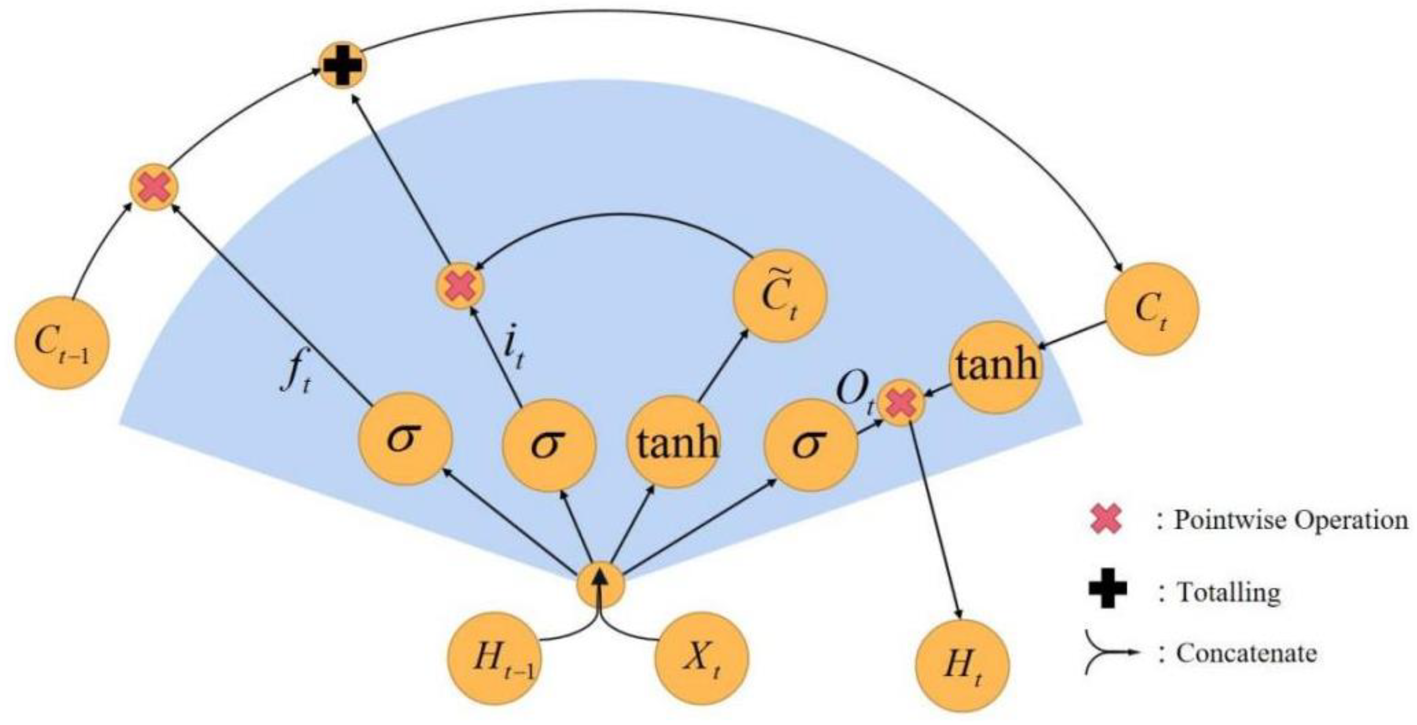
LSTM was first proposed by Hochreiter and Schmidhuber [32]. It can overcome the long computational time, large errors, explosions, or disappearances of data gradients issues of standard RNN networks. The schematic structure of an LSTM network is shown in Figure 1. Ct−1 and Ct are the cell state of the prior nod and the current nod, respectively; is temporary variable of the cell state; Ht−1 and Ht are the hidden layer state of the prior layer and the current layer state; Xt is the input variable; σ and tanh represent activation functions of neurons; the red crosses represent pointwise multiplication operations; the black cross represents the totaling operation; the two lines with one arrow represent concatenate operation; and the two arrows represent copy operation.
Activation functions σ and tanh are used to scale the input vector into a range of [0, 1], and are expressed mathematically as:
where ω and b are the transfer and bias matrices, respectively.
The main difference between an LSTM structure and a standard RNN structure lies in the introduction of memory cell C and gate structures. The gate structures consist of three parts: a forgetting gate, an updating gate, and an output gate. The forgetting gate is expressed using Equation (7), which determines how much information is forgotten in the memory cell by the state of hidden layers at the previous node and at the current input.
where is the hidden state matrix of the last time stamp; sigmoid function σ maps the values to [0, 1]; 1 represents forgetting all; and 0 represents forgetting null.
The update gate is described in Equations (8)–(10). Equation (8) is the input gate of the current memory cell. Equation (9) is the information brought by the current input. The current memory cell is updated with Equation (10), in accordance with the past and present states of the input cell.
where is the coefficient that controls the candidate memory cell to update the memory cell; the candidate memory cell holds short-term dependency information computed from the input matrix .
The output gate is described using Equations (11) and (12). The output current cell state is determined by the hidden layer state of the previous time node and the input node.
2.3. Materials
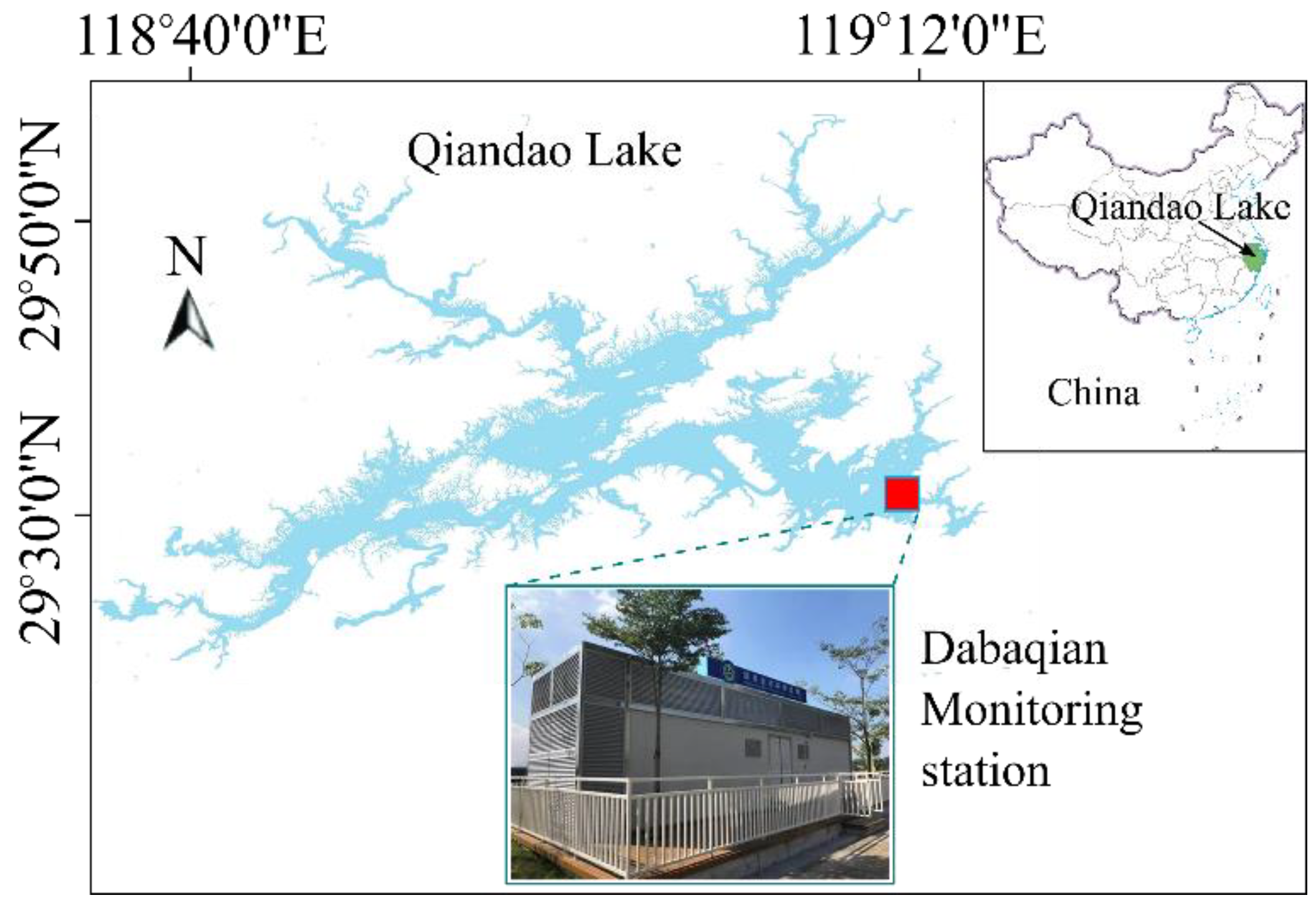
The algorithm of GRA-LSTM is used to predict the water quality of Qiandao Lake, Zhejiang Province, China, based on historical data collected by a monitoring station. Figure 2 shows the geographical location of the monitoring station. The fundamental parameters to assess the water quality include pH, dissolved oxygen (DO), permanganate index (COD), ammonia nitrogen (NH3-N), and total phosphorus (TP). The data were collected for 4 h each day during 2019 and 2020. Table 1 shows the statistic information of measured parameters. Due to occasional malfunctions of some sensors, some data are either abnormal or lost. Such a database is used to verify our GRA-LSTM algorithms.
3. Modeling Flow
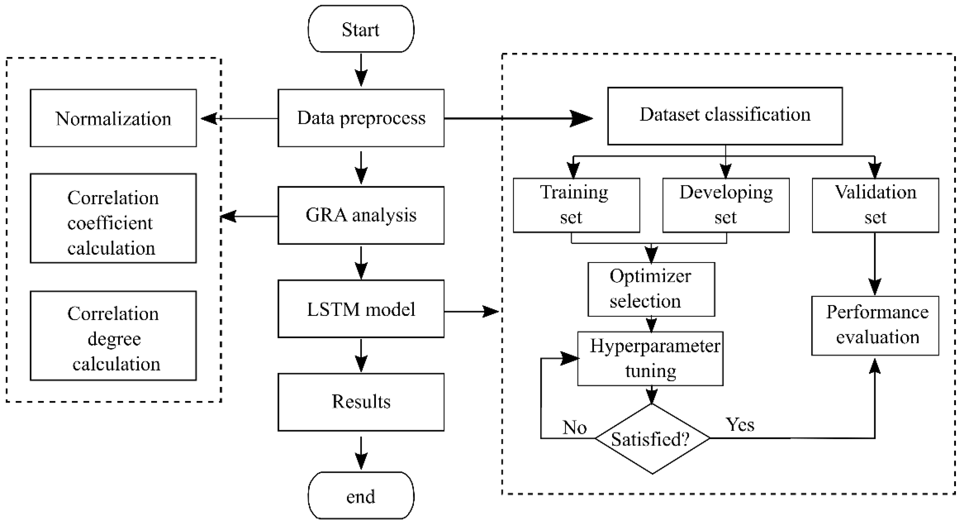
The modeling platform in this study was based on TensorFlow, and the development environment was Python 3.7. Figure 3 shows the flow chat of GRA-LSTM model, the details of which are described in the following four steps.
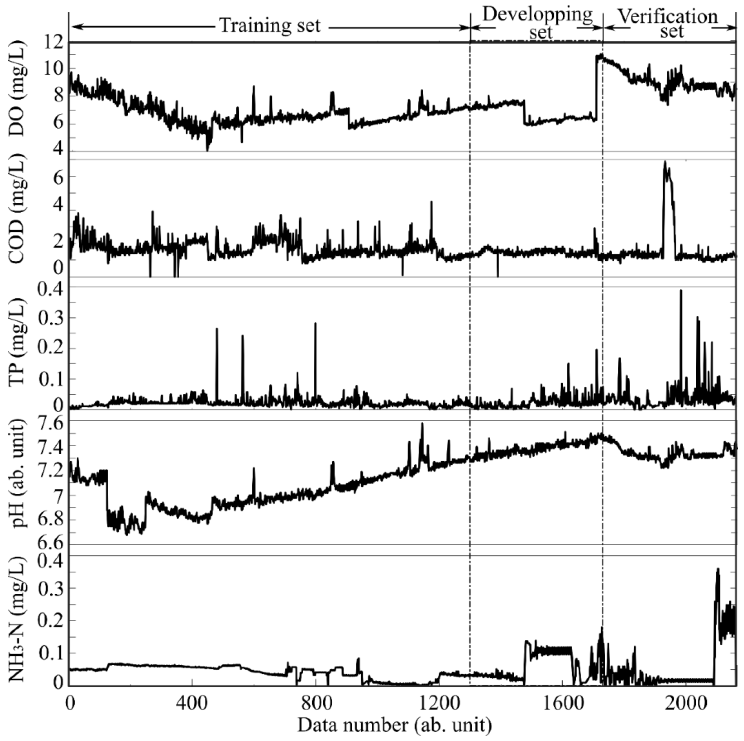
Step 1: Data preprocesses. The missing data from the original dataset are replenished by Lagrange interpolations of adjacent values (missing points are less than 6) or the averaged values of the previous seven (missing points are more than 6). Figure 4 shows the preprocessed data. From Figure 4, we can observe that the concentrations of DO and COD are almost one order of magnitude higher those that of TP and NH3-N. The concentration of TP is close to zero, with the exception of noise-like fluctuations. The sharp rises and falls in the preprocessed data indicate significant changes in water quality, which should be captured by the prediction model and then trigger the warning in advance for water managers.
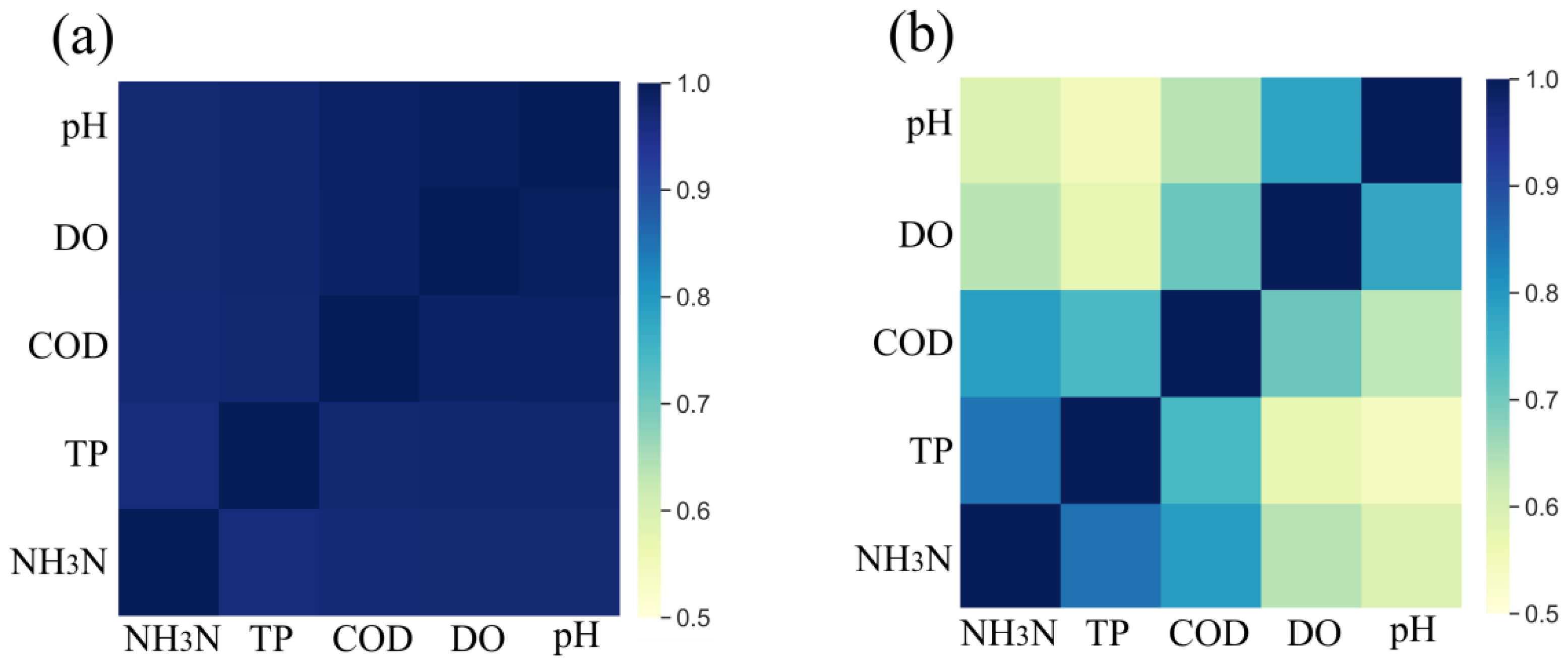
Step 2: GRA model establishment. The preprocessed data are subjected to feature scaling in accordance with Equation (1) or Equation (2), eliminating the magnitudes and units. The grey correlation coefficients and degrees are then calculated according to Equation (3) and Equation (4), respectively. Figure 5 shows calculated grey correlation coefficients using two feature scaling methods. When the original data are scaled by the first data array, as shown in Figure 5a, the coefficients almost reach beyond 0.9. However, when the original data are scaled by the max-min normalization, as shown in Figure 5b, the coefficients span between 0.5 and 1, and the correlations between different quality parameters becomes much more distinguishable. The concentrations of NH3-N, TP, and COD are strongly relevant, while DO and pH are more relevant. Thus, max-min normalization will be used in the GRA process.
Step 3: LSTM model establishment. The data are first divided into three subsets: a training set, a development set, and a validation set, following a typical ratio of 6:2:2 [14]. Since there are 2190 sets of data in total for each water parameter we observed, the sizes of the three datasets are 1314, 438, and 438, respectively, as shown in Figure 4. The measurement data on the previous 12 nodes are used as input data, and the data of the 13th node is used as output data. The output data is further weighted by the grey correlation degree of the other water quality parameters calculated in Step 2. Different optimizers, such as Stochastic Gradient Descent, AdaGrad, and Adaptive Moment Estimation, are applied to adjust the model combining the training set and the development set. Hyper-parameters of the network, including total number of LSTM layer, number of neurons, attenuation coefficient, learning rate, patience value, epoch, and batch side are adjusted according to the root mean square errors (RMSEs) of the water quality parameters. The final hyper-parameters are listed in Table 2.
Step 4: Figure of merit (FOM) evaluations. The fitted model is verified by the verification set. The FOM of the model performance which we used is the RMSE between the verification set and the predicted data from the LSTM networks.
4. Results and Discussions
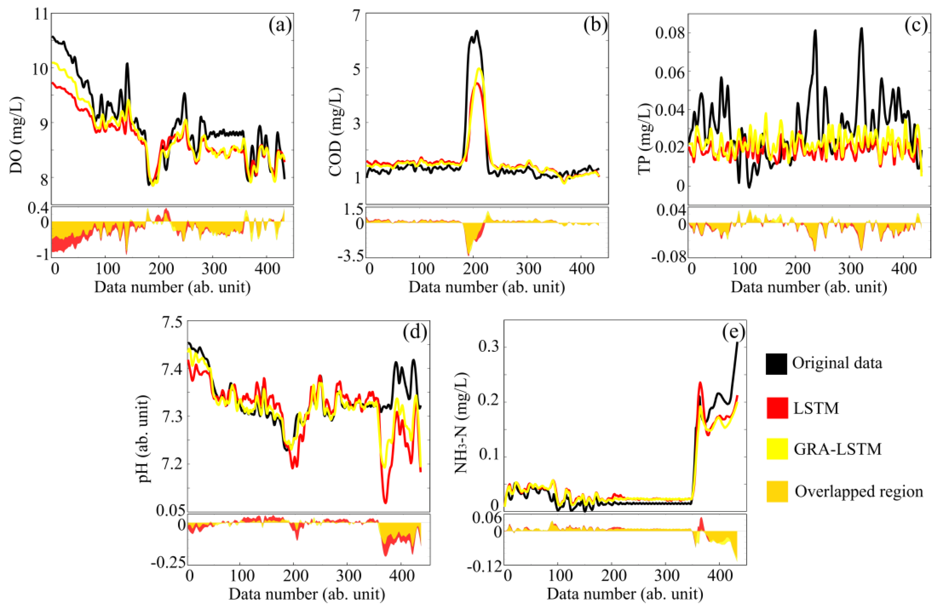
Figure 6 shows the present water quality predictions and their comparisons with the original data. The configurations of the hardware and software, as well as the calculation costs of LSTM and GRA-LSTM, are listed in Table 3. From Table 3, it can be found that the GAR-LSTM model slightly saves computational time, even if the same processor and platform are used. The computation efficiency could be considerable if a significant amount of feeding data were needed.
The parameters of water quality include DO (a), COD (b), TP (c), pH (d), and NH4-N (e), which are predicted using conventional LSTM (red) and GRA-LSTM (yellow) methods. The upper panels in Figure 5 show the comparisons of the predicted data with the original data (black lines), and the lower panels show the residual errors relative to original data using two prediction methods. It should be noted that the regions filled with orange color are the intersections of residual errors using the conventional LSTM (red) and GRA-LSTM (yellow) methods. As can be clearly seen from the upper panels, the predictions generally follow the tendencies of original data, regardless of noise-like fluctuations and sharp changes, validating the feasibility of prediction models. It can also be observed that the residual errors of conventional LSTM are globally larger than those of GRA-LSTM, since the yellow regions in the lower panels of Figure 6a–e are generally covered by the red regions.
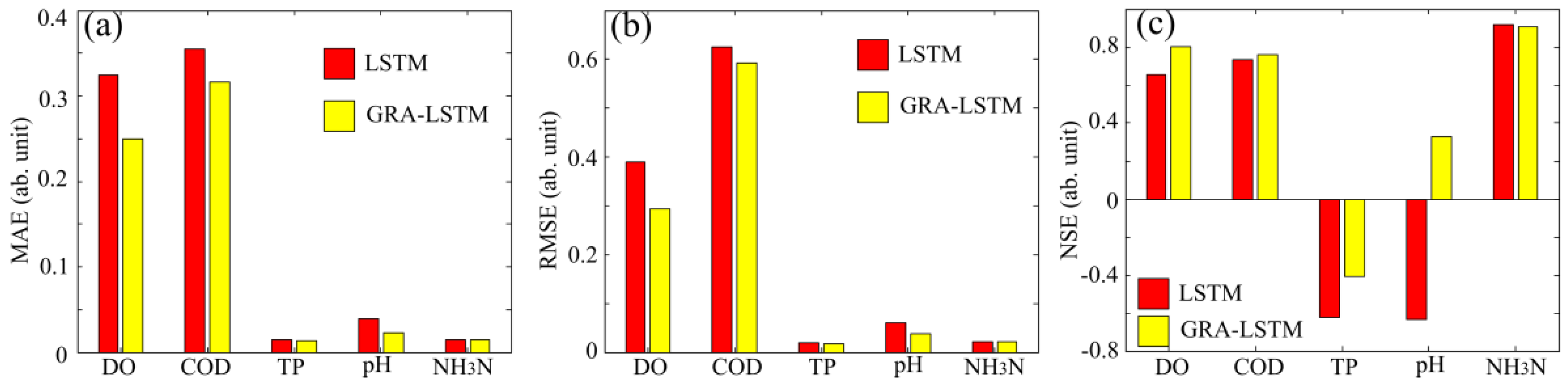
In order to quantify the residual errors from the two prediction models, we calculate the mean absolute errors (MAEs), root mean square errors (RMSEs) and Nash–Sutcliffe efficiency coefficients (NSEs) for each parameter of water quality. As shown in the bar diagram in Figure 7a, the MAEs of GRA-LSTM are globally lower than those of conventional LSTM. The MAEs of five parameters are DO, COD, TP, pH, and NH3-N, and these are reduced by 23.03%, 10.71%, 7.54%, 43.06%, and 1.62% by using the GRA-LSTM algorithm. As for RMSEs, as can be observed in Figure 7b, with the exception of a comparable level in NH3-N, the RMSEs of LSTM are generally higher than those of GRA-LSTM, which can be reduced by 24.47%, 5.28%, 6.92%, and 35.89% for the four parameters: DO, COD, TP, and pH, respectively. We also calculate the NSEs for each water parameter, which statistically denote the relative magnitude of the residual variance compared to the measured data variance. As seen from Figure 7c, with the exception of a slightly lower level in NH3-N, NSEs of the other parameters are higher and closer to 1 when using the GRA-LSTM algorithm, indicating the higher estimation skill of the prediction model. We note that the NSEs of TP are negative, indicating that the two prediction models are unreliable. This is due to the low concentration of TP in the water, which is quite close to the noise level. Based on the above error analyses, we can conclude that GRA-LSTM demonstrates a higher precision and robustness in comparison with conventional LSTM.
Similarly to other kinds of prediction methods based on artificial neural networks [33], GRA-LSTM treats temporal response of multiple parameters as a black box, regardless of its internal physical mechanisms. This implies that GRA-LSTM can treat universe data series, which might show sharp variances and even random distributions. Being different from other neural network-based models, GRA-LSTM does not need a large amount of feeding data. This is because additional correlations of other events occurring in the same time range are implemented. This saves considerable computational resources and time, allowing the possibility of the realizations of real-time predictions. In addition, due to the considerations of other relevant events or factors, the GRA-LSTM algorithm normally shows better immunity to background noises, indicating a higher stability and robustness compared with other neural network-based methods. This has been demonstrated in the comparison of NSEs. On the other hand, each data series predicted by GRA-LSTM is dependent and are limited to the situations in which the measurements are multiple dimensionalities.
5. Conclusions
By combining conventional LSTM networks with GRA correlation models, an improved GRA-LSTM algorithm was developed in order to better predict the real-time quality of drinking water. A total of 2190 sets of monitoring data were collected from monitoring stations in the Qiandao Lake, China, from 2019 to 2020, and these served as feeding datasets. Each dataset was divided into a ratio of 6:2:2, each of which served as training set, development set, and validation set, for the purpose of dynamic self-corrections. GRA degree coefficients between different water quality parameters were used to correct the weight factors of LSTM networks. Compared with conventional LSTM models, the MAEs of four key parameters of water quality, DO, COD, TP, and pH, were reduced by 23.03%, 10.71%, 7.54%, and 43.06%, respectively, while corresponding RMSEs were reduced by 24.47%, 5.28%, 6.92%, and 35.89%, respectively. Combining GRA and conventional LSTM algorithms, the GRA-LSTM is proposed to treat discrete events, using a small amount of feeding datasets and multiple correlated events in the same time range. The prediction precision and robustness are further enhanced by the implementation of correlation coefficients to serve as the weight factors at each node of neural networks. We envision that other mathematical models, such as Markov chains and Kalman recursions, could be further implemented into the node of our GRA-LSTM or for more generalized artificial neural networks, in order to better cope with discrete events with sequential correlations.
Author Contributions
X.T.: conceptualization, methodology, validation, formal analysis, investigation, writing—original draft, writing—review and editing, project administration, funding acquisition. Z.W.: conceptualization, methodology, formal analysis, investigation, writing—original draft, writing—review and editing. E.T.: conceptualization, methodology, formal analysis, writing—original draft, writing—review and editing. B.Z.: conceptualization, methodology, formal analysis, investigation, writing—original draft, writing—review and editing. X.L.: conceptualization, methodology, formal analysis, investigation, writing—review and editing, resources, visualization, project administration, funding acquisition. J.W.: conceptualization, methodology, validation, investigation, writing—review and editing. M.C.O.: conceptualization, methodology, investigation, writing—review and editing. Z.Z.: conceptualization, methodology, writing—review and editing, funding acquisition. All authors have read and agreed to the published version of the manuscript.
Funding
This work was supported by the National Natural Science Foundation of China (No. 51709070), Key R&D Program of Zhejiang Province (No. 2021C03013), and the Fundamental Research Funds for the Provincial Universities of Zhejiang (No. GK229909299001-007).
Acknowledgments
We thank Pengfei Jiao from Hangzhou Dianzi University for the assistance of computational programming.
Conflicts of Interest
The authors declare no conflict of interest.
References
- Cao, J.; Sun, Q.; Zhao, D.; Xu, M.; Shen, Q.; Wang, D.; Wang, Y.; Ding, S. A critical review of the appearance of black-odorous waterbodies in China and treatment methods. J. Hazard. Mater. 2020, 385, 121511. [Google Scholar] [CrossRef] [PubMed]
- Liu, S.; Tai, H.; Ding, Q.; Li, D.; Xu, L.; Wei, Y. A hybrid approach of support vector regression with genetic algorithm optimization for aquaculture water quality prediction. Math. Comput. Model. 2013, 58, 458–465. [Google Scholar] [CrossRef]
- Elçi, Ş. Effects of thermal stratification and mixing on reservoir water quality. Limnology 2008, 9, 135–142. [Google Scholar] [CrossRef] [Green Version]
- Karthik, L.; Kumar, G.; Keswani, T.; Bhattacharyya, A.; Chandar, S.S.; Bhaskara Rao, K.V. Optimised neural network model for river-nitrogen prediction utilizing a new training approach. PLoS ONE 2020, 15, e0239509. [Google Scholar] [CrossRef]
- Han, X.; Liu, X.; Gao, D.; Ma, B.; Gao, X.; Cheng, M. Costs and benefits of the development methods of drinking water quality index: A systematic review. Ecol. Indic. 2022, 144, 109501. [Google Scholar] [CrossRef]
- Tyralis, H.; Papacharalampous, G.; Langousis, A. A brief review of random forests for water scientists and practitioners and their recent history in water resources. Water 2019, 11, 910. [Google Scholar] [CrossRef] [Green Version]
- Eze, E.; Halse, S.; Ajmal, T. Developing a Novel Water Quality Prediction Model for a South African Aquaculture Farm. Water 2021, 13, 1782. [Google Scholar] [CrossRef]
- Lu, H.; Ma, X. Hybrid decision tree-based machine learning models for short-term water quality prediction. Chemosphere 2020, 249, 126169. [Google Scholar] [CrossRef]
- Maier, H.R.; Dandy, G.C. The use of artificial neural networks for the prediction of water quality parameters. WRR 1996, 32, 1013–1022. [Google Scholar] [CrossRef]
- Yahya, A.S.A.; Ahmed, A.N.; Othman, F.B.; Ibrahim, R.K.; Afan, H.A.; El-Shafie, A.; Fai, C.M.; Hossain, S.; Ehteram, M.; Elshafie, A. Water quality prediction model based support vector machine model for ungauged river catchment under dual scenarios. Water 2019, 11, 1231. [Google Scholar] [CrossRef]
- Chen, S.; Fang, G.; Huang, X.; Zhang, Y. Water quality prediction model of a water diversion project based on the improved artificial bee colony–backpropagation neural network. Water 2018, 10, 806. [Google Scholar] [CrossRef] [Green Version]
- Dauji, S.; Rafi, A. Spatial interpolation of SPT with artificial neural network. Eng. J. 2021, 25, 109–120. [Google Scholar] [CrossRef]
- Daosud, W.; Hussain, M.A.; Kittisupakorn, P. Neural network-based hybrid estimator for estimating concentration in ethylene polymerization process: An applicable approach. Eng. J. 2020, 24, 29–39. [Google Scholar] [CrossRef]
- Abiodun, O.I.; Jantan, A.; Omolara, A.E.; Dada, K.V.; Mohamed, N.A.; Arshad, H. State-of-the-art in artificial neural network applications: A survey. Heliyon 2018, 4, e00938. [Google Scholar] [CrossRef] [Green Version]
- Haghiabi, A.H.; Nasrolahi, A.H.; Parsaie, A. Water quality prediction using machine learning methods. WQRJ 2018, 53, 3–13. [Google Scholar] [CrossRef]
- Aldhyani, T.H.H.; Al-Yaari, M.; Alkahtani, H.; Maashi, M. Water quality prediction using artificial intelligence algorithms. Appl. Bionics Biomech 2020, 2020, 6659314. [Google Scholar] [CrossRef]
- Zhang, H.; Wang, Z.; Liu, D. A comprehensive review of stability analysis of continuous-time recurrent neural networks. IEEE Trans. Neural Netw. Learn. Syst. 2014, 25, 1229–1262. [Google Scholar] [CrossRef]
- Farhi, N.; Kohen, E.; Mamane, H.; Shavitt, Y. Prediction of wastewater treatment quality using LSTM neural network. Environ. Technol. Innov. 2021, 23, 101632. [Google Scholar] [CrossRef]
- Zhang, S.; Lan, X.; Yao, H.; Zhou, H.; Tao, D.; Li, X. LSTM: A search space odyssey. IEEE Trans. Neural Netw. Learn. Syst. 2016, 28, 2222–2232. [Google Scholar] [CrossRef] [Green Version]
- Hu, Y.-L.; Chen, L. A nonlinear hybrid wind speed forecasting model using LSTM network, hysteretic ELM and Differential Evolution algorithm. Energy Convers. Manag. 2018, 173, 123–142. [Google Scholar] [CrossRef]
- Rasheed Abdul Haq, K.P.; Harigovindan, V.P. Water quality prediction for smart aquaculture using hybrid deep learning models. IEEE Access 2022, 10, 60078–60098. [Google Scholar] [CrossRef]
- Liu, P.; Wang, J.; Sangaiah, A.K.; Xie, Y.; Yin, X. Analysis and prediction of water quality using LSTM deep neural networks in IOT environment. Sustainability 2019, 11, 2058. [Google Scholar] [CrossRef] [Green Version]
- Liu, S.F.; Dang, Y.G.; Fang, Z.G. Grey System Theory and Its Applications, 3rd ed.; Science Press: Beijing, China, 2011. [Google Scholar]
- Jin, X.; Du, J.; Liu, H.; Wang, Z.; Song, K. Remote estimation of soil organic matter content in the Sanjiang plain, Northeast China: The optimal band algorithm versus the GRA-ANN model. Agric. ForMeteorol. 2016, 218, 250–260. [Google Scholar] [CrossRef]
- Wei, G.-W. GRA method for multiple attribute decision making with incomplete weight information in intuitionistic fuzzy setting. KBS 2010, 23, 243–247. [Google Scholar] [CrossRef]
- Li, L.; Jiang, P.; Xu, H.; Lin, G.; Guo, D.; Wu, H. Water quality prediction based on recurrent neural network and improved evidence theory: A case study of Qiantang River, China. ESPR 2019, 26, 19879–19896. [Google Scholar] [CrossRef]
- Ip, W.; Hu, B.; Wong, H.; Xia, J. Applications of grey relational method to river environment quality evaluation in China. J. Hydrol. 2009, 379, 284–290. [Google Scholar] [CrossRef]
- Wei, G.W. Gray relational analysis method for intuitionistic fuzzy multiple attribute decision making. Expert Syst. Appl. 2011, 38, 11671–11677. [Google Scholar] [CrossRef]
- Li, X.; Zhang, Y.; Yin, K. A new grey relational model based on discrete Fourier transform and its application on Chinese marine economic. MAEM 2018, 1, 79–100. [Google Scholar] [CrossRef]
- Zhou, J.; Wang, Y.; Xiao, F.; Wang, Y.; Sun, L. Water quality prediction method based on IGRA and LSTM. Water 2018, 10, 1148. [Google Scholar] [CrossRef] [Green Version]
- Julong, D. Introduction to grey system theory. J. Grey Syst. 1989, 1, 1–24. [Google Scholar] [CrossRef]
- Hochreiter, S.; Schmidhuber, J. Long Short Term Memory. Neural Comput. 1997, 9, 1735–1780. [Google Scholar] [CrossRef] [PubMed]
- Valis, D.; Hasilova, K.; Forbelska, M.; Pietrucha-Urbanik, K. Modelling water distribution network failures and deterioration. In Proceedings of the IEEE International Conference on Industrial Engineering and Engineering Management, Singapore, 10–13 December 2017; pp. 924–928. [Google Scholar] [CrossRef]
Figure 1.
Schematic LSTM network structure.

Figure 2.
Geographical position of the water quality monitoring station.

Figure 3.
Flow chart of GRA-LSTM model.

Figure 4.
Preprocessed original data of water quality parameters.

Figure 5.
Grey correlation coefficients using two scaling methods. (a) Original data are scaled by the first data array; (b) original data are scaled by the max-min normalization.
Figure 5.
Grey correlation coefficients using two scaling methods. (a) Original data are scaled by the first data array; (b) original data are scaled by the max-min normalization.

Figure 6.
Water quality predictions and their comparisons with original data. (a) DO; (b) COD; (c) TP; (d) pH; (e) NH3-N.
Figure 6.
Water quality predictions and their comparisons with original data. (a) DO; (b) COD; (c) TP; (d) pH; (e) NH3-N.

Figure 7.
Error analyses using LSTM and GRA-LSTM methods. (a) MAE comparisons; (b) RMSE comparisons; (c) NSE comparisons.
Figure 7.
Error analyses using LSTM and GRA-LSTM methods. (a) MAE comparisons; (b) RMSE comparisons; (c) NSE comparisons.


Table 1.
Water quality information statistics.
| Water Quality Parameters | DO (mg/L) | NH3-N(mg/L) | pH | COD (mg/L) | TP (mg/L) |
|---|---|---|---|---|---|
| Minimum value | 4.05 | 0 | 6.68 | 0.8 | 0 |
| Maximum value | 11.05 | 0.36 | 7.58 | 6.90 | 0.39 |
| Average value | 7.24 | 0.048 | 7.16 | 1.62 | 0.025 |
| Standard deviation | 1.261 | 0.044 | 0.206 | 0.684 | 0.024 |
| Skewness | 0.819 | 2.762 | −0.394 | 4.082 | 6.111 |
Table 2.
Hyper-parameter settings.
| Hyperparameters | DO | NH3-N | pH | COD | TP |
|---|---|---|---|---|---|
| Total number of LSTM layers | 4 | 4 | 4 | 4 | 4 |
| Number of neurons | 100 | 100 | 100 | 100 | 100 |
| Attenuation coefficient | 0.8 | 0.1 | 0.6 | 0.6 | 0.1 |
| Learning rate | 0.0001 | 0.0001 | 0.0001 | 0.0001 | 0.001 |
| Patience values | 2 | 5 | 2 | 15 | 5 |
| Epoch | 200 | 200 | 200 | 200 | 200 |
| Batch size | 128 | 8 | 16 | 64 | 8 |
Table 3.
Hardware and software configurations.
| Algorithm | LSTM | GRA-LSTM |
|---|---|---|
| Processor | Core i7-6700HQ CPU: 8 | Core i7-6700HQ CPU: 8 |
| Configurations | Windows 10 + python3.7 | Windows 10 + python3.7 |
| Calculation time | 220.5 s | 219.4 s |
Publisher’s Note: MDPI stays neutral with regard to jurisdictional claims in published maps and institutional affiliations. |
© 2022 by the authors. Licensee MDPI, Basel, Switzerland. This article is an open access article distributed under the terms and conditions of the Creative Commons Attribution (CC BY) license (https://creativecommons.org/licenses/by/4.0/).
Share and Cite
MDPI and ACS Style
Tian, X.; Wang, Z.; Taalab, E.; Zhang, B.; Li, X.; Wang, J.; Ong, M.C.; Zhu, Z. Water Quality Predictions Based on Grey Relation Analysis Enhanced LSTM Algorithms. Water 2022, 14, 3851. https://doi.org/10.3390/w14233851
AMA Style
Tian X, Wang Z, Taalab E, Zhang B, Li X, Wang J, Ong MC, Zhu Z. Water Quality Predictions Based on Grey Relation Analysis Enhanced LSTM Algorithms. Water. 2022; 14(23):3851. https://doi.org/10.3390/w14233851
Chicago/Turabian StyleTian, Xiaoqing, Zhenlin Wang, Elias Taalab, Baofeng Zhang, Xiaodong Li, Jiyong Wang, Muk Chen Ong, and Zefei Zhu. 2022. "Water Quality Predictions Based on Grey Relation Analysis Enhanced LSTM Algorithms" Water 14, no. 23: 3851. https://doi.org/10.3390/w14233851
Note that from the first issue of 2016, this journal uses article numbers instead of page numbers. See further details here.