Bridging the Data Gap between the GRACE Missions and Assessment of Groundwater Storage Variations for Telangana State, India

Abstract

Because of changing climatic conditions, uneven distribution of rainfall occurs throughout India. As a result, dependence on groundwater for irrigation has increased tremendously for industrial and domestic purposes. In India approximately 89% of agricultural demands are met through groundwater. Due to increases in population, demand for groundwater and lack of effective utilization have resulted in rapid depletion of groundwater in most parts of the country. Therefore, quantifying groundwater resources is a serious concern in populated states of India, because it is now difficult to supply enough water to every citizen, and will remain so in the future. Because of difficulties in accessing observation data, researchers have begun to depend on satellite-based remote sensing information to deal with groundwater variations. The present study deals with filling the data gap between Gravity Recovery And Climate Experiment (GRACE) and GRACE Follow On (GRACE FO) missions using multilayer perceptron’s (MLPs) during 2017–2018 to obtain a continuous terrestrial water storage anomaly (TWSA) series from 2003 to 2020 for Telangana state, India. The MLP model performed well in predicting the TWSA, with a correlation coefficient of r = 0.96 between modeled TWSA and GRACE TWSA during the test period. Telangana state observed negative TWSAs (annual) in the years 2003, 2004, 2005, 2009, 2012, 2015, and 2016–19. This TWSA series (2003–2020) was then used to evaluate regional groundwater storage anomalies (GWSAs) in Telangana state, which is considered to be one of the water stress regions in India. The TWSAs were converted to GWSAs using Global Land Data Assimilation System (GLDAS) parameters. The Telangana state experienced decreasing GWSA in the years 2005, 2009, and 2012, and from 2015 to 2019, leading to severe droughts. Groundwater well measurements were obtained from the Central Groundwater Board (CGWB) and converted to GWSA at a seasonal scale. The GWSAs obtained from GRACE (GWSA_GRACE) were converted to seasonal values and compared with GWSAs obtained from observation well data (GWSA_obs). The performance metrics of r = 0.74, RMSE = 5.3, and NSE = $0.62$ were obtained between (GWSA_GRACE) and (GWSA_obs), representing a good correlation among them. Over the past decade, Telangana state has significantly relied on groundwater resources for irrigation, domestic, and industrial purposes. As a result, evaluating groundwater storage variations at a regional scale may help policy makers and water resource researchers in the sustainable utilization and management of groundwater resources.

1. Introduction

In India, groundwater is the most preferred source for irrigation, domestic, and industrial purposes because of its easy availability and low capital cost. In India, groundwater is a valuable natural water resource because it meets approximately 89% of agricultural demands [1]. This percentage will increase further as the population of the country increases. The country’s growing dependance on groundwater has led to indiscriminate extraction in different regions throughout India, without proper consideration of recharge of aquifers and other issues related to the environment, resulting in rapid depletion of groundwater in most parts of the country [2,3]. The situation has worsened due to uncertainties in the seasonal water availability caused by climate change, in addition to rising food demand met by irrigation and agriculture [4,5].

India accounts for 18% of the world’s population and 30% of the world’s irrigated land [1,6]. Groundwater sources provide about 85% of drinking water in rural areas and a significant percentage of it in urban areas [7]. Due to a growing population, rapid urbanization, and changing lifestyles, India is experiencing a severe shortage of water, in addition to a sharp increase in water demand. The present study deals with groundwater storage variations in Telangana state, for which the largest river systems include Godavari in the north and Krishna in the south. Other river systems include Bhima, Penganga, and Manair. However, the groundwater availability of the study area is rather uneven, with aquifers ranging from crystalline to sedimentary aquifers [1]. Moreover, due to the uneven distribution of rainfall because of climate change, groundwater usage has increased tenfold in different parts of the country [8,9,10].

Different climate zones, from the driest to some of the wettest regions on Earth, exist in India based on the pattern of differential precipitation [1]. A large portion of the region is classified as highly water stressed because of extensive abstraction of the available groundwater [11]. According to earlier research, India’s groundwater resources may be seriously threatened if withdrawal continues at this rate [12]. The reasons for depletion include ineffective water usage habits, poorly maintained irrigation systems, and insufficient water and power prices, which encourage the misuse of water [13]. Therefore, quantifying groundwater resources is a serious concern in populated states of India, because it is now difficult to supply enough water to every citizen, and will remain so in the future.

For scientists and water resource managers, predicting groundwater availability in India has become harder. In addition to difficulties with accessing observation data from governmental organizations, this is partially caused by data-related issues such a shortage of field stations, and scarcity of sufficient quantitative and qualitative data. As a result, to estimate ground water variations, researchers have begun to depend on satellite-based remote sensing outputs [9,14]. Using satellite-based observations, previous studies have reported depletion of groundwater storage (GWS) in most parts of the country [2,15,16].

GRACE, a joint United States–German mission, meticulously tracked changes in Earth’s gravity field from 2002 to 2017, and GRACE Follow On (GRACE FO) did so from 2018 to the present [14,17]. Terrestrial water storage changes can be estimated once the influences of atmospheric and oceanic circulation, in addition to solid earth processes, have been removed from gravitational fields [18]. Using a spherical harmonics-based methodology, GRACE produced worldwide maps of TWS anomalies with a horizontal resolution of about 400 km [19]. Recent mass concentration (mascon)-based products have increased accuracy, with horizontal resolutions close to 300 km [20,21].

The GRACE mission started in the 2002 and ended in 2017. Then, the GRACE FO mission provided the changes in the Earth’s gravity field from 2018 to the present. Between the GRACE and GRACE FO missions, an 11-month gap exists due to the change in missions. Temporal GRACE data are not continuous due to this 11-month gap. Therefore, to obtain a continuous dataset of GRACE gravity fields, numerous researchers have tried to fill this gap using statistical and artificial intelligence methods. Ref. [22] filled the gap between the two missions using a hydrological model. Ref. [23] filled this gap using artificial neural networks. Ref. [24] reconstructed GRACE TWSA before 2002 using machine learning methods. The continuous GRACE series can be utilized to assess long-term TWS variations and for climate-related studies.

Previously, many studies have used GRACE observations to evaluate GWS variations in Indian states. Ref. [14] evaluated GRACE GWS variations and compared them with in situ observation well measurements in Rajasthan, Haryana, and Punjab. Ref. [25] calculated GWS variations using GRACE and validated the results with in situ groundwater observation well-based storage for Indian river systems. Ref. [26] calculated GWS variations for Indian lakes and their relationship with ENSO events. Ref. [27] studied GWS variations related to aquifer systems for Maharashtra state, India. Ref. [28] evaluated GWS variations using GRACE and GLDAS for Tamilnadu State, India. Ref. [29] studied the water storage dynamics using GRACE, hydrological models, and in situ observations for Peninsular India. Ref. [30] applied data assimilation using GRACE and a land surface model in India.

Recent advancements in machine learning techniques have provided new options in hydrology and related domains [31]. The development of machine learning technology has substantially enhanced our ability to mimic and forecast the global environment. Machine learning approaches have been shown to be effective in solving the most challenging tasks, such as data prediction and reconstruction. Machine learning techniques, such as artificial neural networks, deep convolutional neural networks, multiple linear regression, and autoregressive exogenous models, have been used to reconstruct GRACE TWSA in recent years [32,33,34,35]. In addition, methods such as extreme gradient boosting, the integrated machine learning model optimized by the whale algorithm, deep learning, and ensemble deep learning have been adopted to predict groundwater levels for different regions of the world [36,37,38].

At a regional level, GRACE-based estimates have been useful in assessing groundwater variations [17]. Earlier research documented rapid groundwater storage depletion at regional and basin scales throughout the world using a satellite-based methodology [39,40]. Similar studies have utilized GRACE data to represent groundwater depletion in different parts of the world [41,42,43]. Ground-based estimates must be used to assess satellite data products in order to enhance algorithms for data retrieval approaches. GRACE results require additional validation studies worldwide since GRACE gravity processing methods are constantly changing over time [20]. There are very few studies that have compared GRACE groundwater storage estimations with observation well networks for India [44,45,46].

Due to a sharp decrease in per capita water availability, India is recognized as a future problem area in terms of shortage of water and food insecurity [47]. Over the past decade, Telangana state has relied heavily on groundwater resources for irrigation, domestic, and industrial purposes. As a result, evaluating groundwater storage variations at the regional scale may help policy makers and water resource researchers in the sustainable utilization and management of groundwater resources. In this study, the gap between GRACE and GRACE FO missions was filled using multilayer perceptron’s, and analysis of groundwater storage variations was carried out for Telangana state from 2003 to 2020. Assessment of GRACE GWSAs and validation using ground data have been previously carried out in some Indian regions, such as Gujarat, North-West India, and the Gangetic basin [44,46]. However, no studies have been specifically conducted to fill the gap between GRACE and GRACE FO missions, and to evaluate groundwater storage for Telangana state. The objectives of this study were to: (i) fill the data gap between GRACE and GRACE FO missions using multilayer perceptron’s to obtain a continuous dataset from 2003 to 2020 for Telangana state, India; (ii) analyze GRACE TWSAs at spatial and temporal scales and convert them to groundwater storage anomalies (GWSAs) using a land surface model from 2003 to 2020; (iii) analyze observation well measurements at spatial and temporal scales and convert them into groundwater storage anomalies; and (iv) validate the GRACE GWSAs with observation well-based GWSAs for Telangana state from 2003 to 2020. To the best of our knowledge, this is the first study to fill the data gap between the two missions, to evaluate spatial and temporal GRACE groundwater storage changes, and to validate the results using an extensive network of in situ observation well data gathered throughout Telangana state. The results of this study will help hydrologists choose the best GRACE options for hydrologic applications in studies of regional basins.

2. Material and Methods

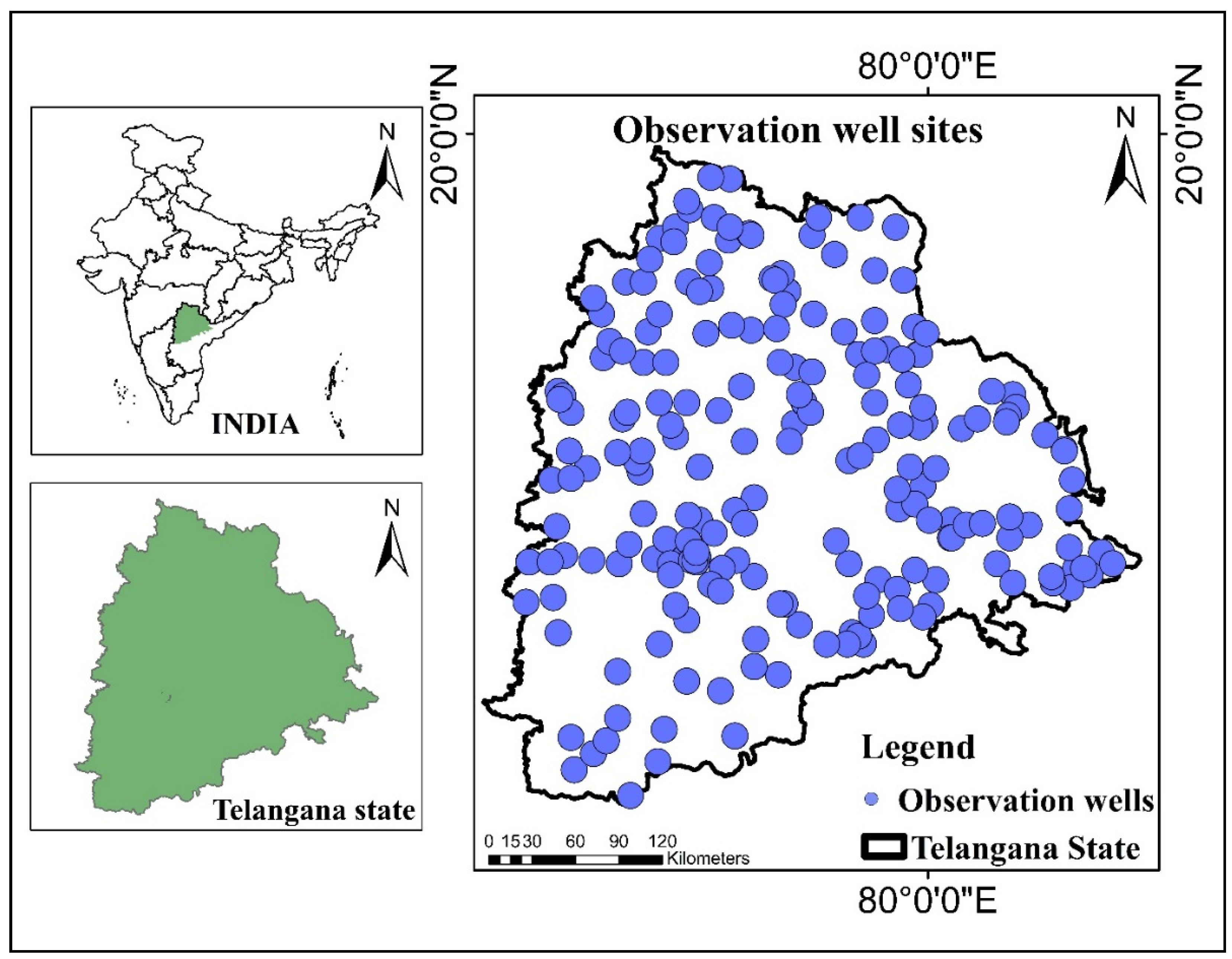
2.1. Study Area

Telangana state, which has a geographical size of 112,077 km², was the 29th state formed in India. It is situated between EL 77°12’ and 81°50’ and NL 15°48’ and 19°54’. Maharashtra, Chattisgarh, Karnataka, and Andhra Pradesh border the state on its eastern, southern, and northern borders, respectively, as shown in Figure 1. Telangana state is mainly drained by two river basins, namely, Godavari and Krishna, and their tributaries. The state is physio-graphically occupied by western Pedi plains and Eastern Ghats. The state contains a wide range of soil types, including lateritic soils, black cotton soils, and red soil. Geographically, Telangana state is in a semi-arid area with a climate that is primarily hot and dry. The normal annual rainfall is 939 mm and average temperature is 42 °C. The average ground water level of the state is 11.14 mbgl [48].

2.2. Data

2.2.1. Gravity Recovery and Climate Experiment (GRACE)

Launched on 17 March 2002, the GRACE twin satellites continuously measure the changes in the Earth’s gravity fields and provide data regarding reservoir storage over land, in addition to ice, ocean, and earthquake data. Two types of GRACE products are available, namely, spherical harmonics (SH) and mass concentrations (mascons). In the present study, the latest release of GRACE monthly mascons (RL 06) processed at the Jet Propulsion Laboratory (JPL) (https://grace.jpl.nasa.gov, accessed on 20 February 2022) were used for the evaluation of terrestrial and groundwater storage. Before using the SH data, the signal strength needs to be reduced in order to smooth it out. In contrast, the analysis can be done directly using the mascon data. The GRACE mission dataset is accessible from 2002 to 2017; however, the mission was inactive from 2017 to 2018. From 2018 until the present, the GRACE FO mission has reported changes in the Earth’s gravitational field. The GRACE mascon terrestrial water storage (TWS) dataset was considered from 2003 to 2017, and GRACE FO was considered from 2018 to 2020, with a spatial resolution of 0.5 × 0.5 at a monthly time scale.

2.2.2. Global Land Data Assimilation System (GLDAS)

GLDAS produces the optimal fields of land surface states and fluxes by utilizing satellite-based and ground-based data products with the help of land surface models and data assimilation techniques [49]. The latest release of GLDAS Noah model i.e., NOAH10_M 2.1, products that are consistent with GRACE product was adopted from 2003 to 2020 and used in this study with a spatial resolution of 1° × 1° (https://disc.gsfc.nasa.gov/ accessed on 15 February 2022). The GLDAS Noah model products, namely, soil moisture and canopy water storage, were considered from 2003 to 2020. To ensure GLDAS products were consistent with the GRACE products, the baseline period was considered from January 2004 to December 2009, which is the same as that of GRACE. By integrating soil moisture storage (ΔSM) and canopy water storage (ΔCWS) from GLDAS, TWSAs were analyzed [35]. The groundwater storage (ΔGW) component, which is absent from the GLDAS Noah product, was obtained from the GLDAS Catchment Land Surface Model (CLSM), which has a daily resolution of 0.25° × 0.25°. Monthly anomalies were then produced by subtracting the mean value for the years 2004 to 2009 [50]. The limitation of CLSM groundwater storage is that it simulates only shallow groundwater storage. GLDAS Noah-based TWSA and CLSM-based groundwater storage were utilized as predictors for GRACE TWSA reconstruction since GLDAS products are as reliable as GRACE products.

2.2.3. In Situ Groundwater Observation Well Measurements

In this study, in situ groundwater well measurements from 210 locations covering Telangana state were considered from 2003 to 2020, as shown in Figure 1. The Central Ground Water Board (CGWB, India) provides the observation well measurements for India for four seasons, namely, (i) post-monsoon rabi (January), (ii) pre-monsoon (May), (iii) monsoon (August), and (iv) post-monsoon kharif (November). The seasonal groundwater data were considered in such a way that, out of the four seasons, at least three were available.

2.3. Method

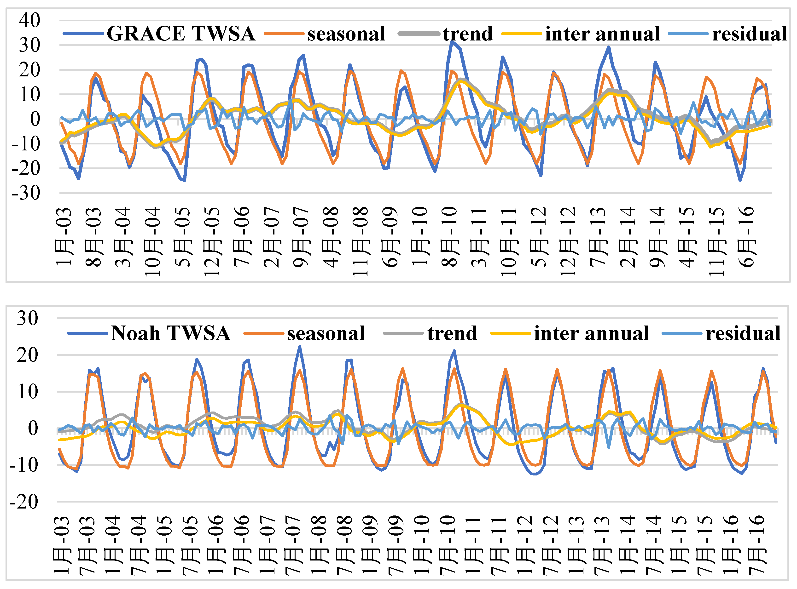
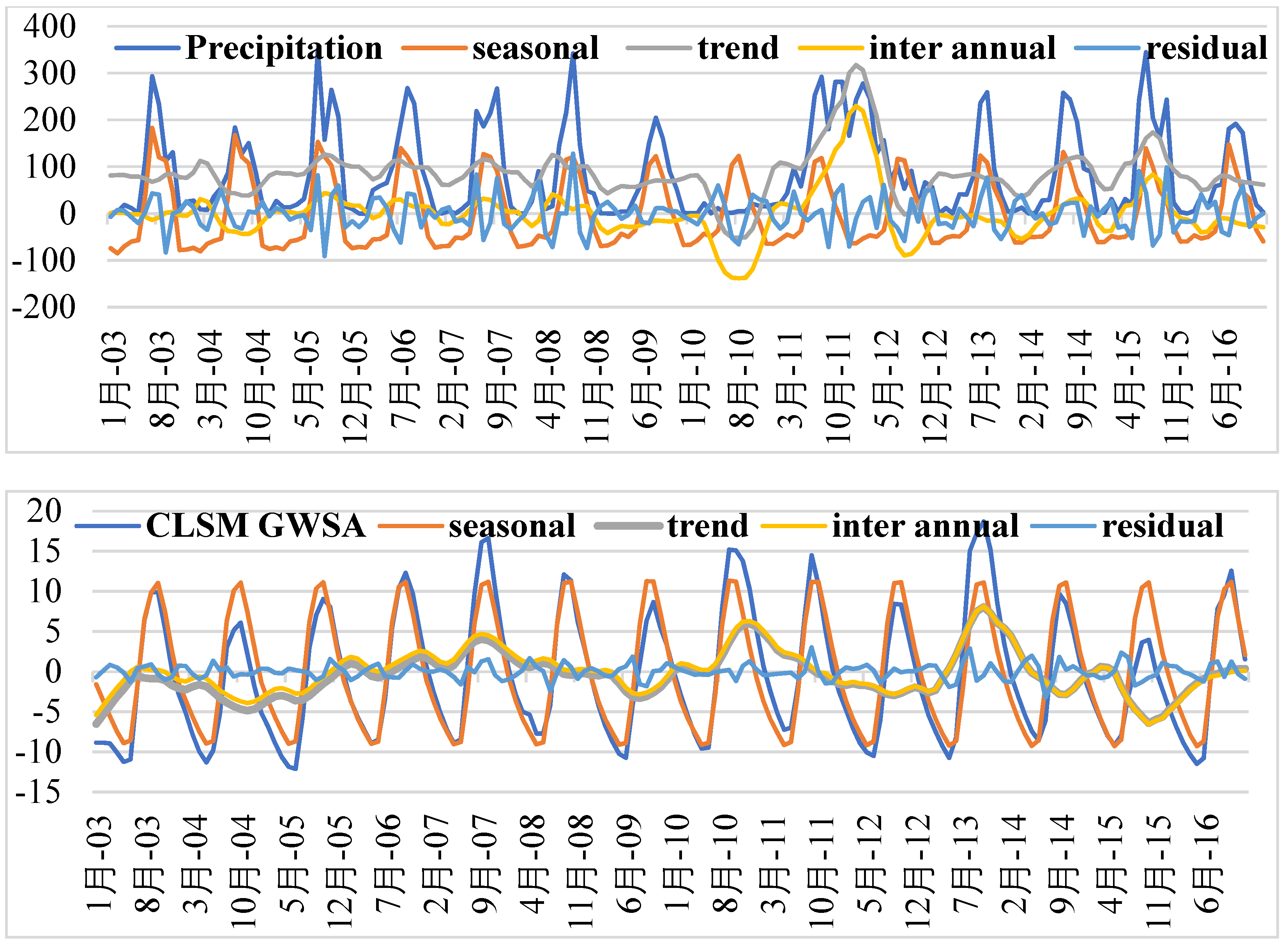
2.3.1. Time Series Decomposition

Decomposition of the GRACE hydrological signal has been a frequent practice in recent literature, with a number of methodologies being used to achieve different objectives. The approach that is most frequently used to separate the various modes of GRACE and forcing data into independent components is Seasonal Trend Decomposition using Loess Procedure (STL), which was first presented by [51]. The STL technique is a reliable and computationally effective approach for identifying non-linear patterns in trend estimations by employing locally weighted regression.

This technique has been used by numerous researchers to break down GRACE TWSAs. This method was employed by [52] to contrast monthly GRACE TWSAs with rainfall time series. This technique was used to separate the GRACE time series into long-term, seasonal, and sub-seasonal portions by [34,53]. The monthly GRACE TWSAs and forcing datasets were subjected to the STL decomposition procedure in this work, producing decomposed time series for each dataset. The time series was divided into three sections using the STL method: trend (in this case, interannual and linear trend portions), seasonal, and residual parts:

$$Y=T^c+S^c+R^c$$

(1)

where, $Y$ represents time series (GRACE TWSA and forcing datasets), $T^c$ represents the trend part, $S^c$ represents the seasonal part, and $R^c$ represents the residual part respectively. $c$ is the cycle-index in the inner loop. The trend part includes interannual and linear components. Using the linear regression method linear trend is separated from $T^c$ and the interannual is generated by subtracting the linear trend from $T^c$ (Interannual = $T^c$ − linear trend). Then the equation 1 becomes:

$$Y=L^c+I^c+S^c+R^c$$

(2)

where $L^c$ = linear trend and $I^c$ = interannual components.

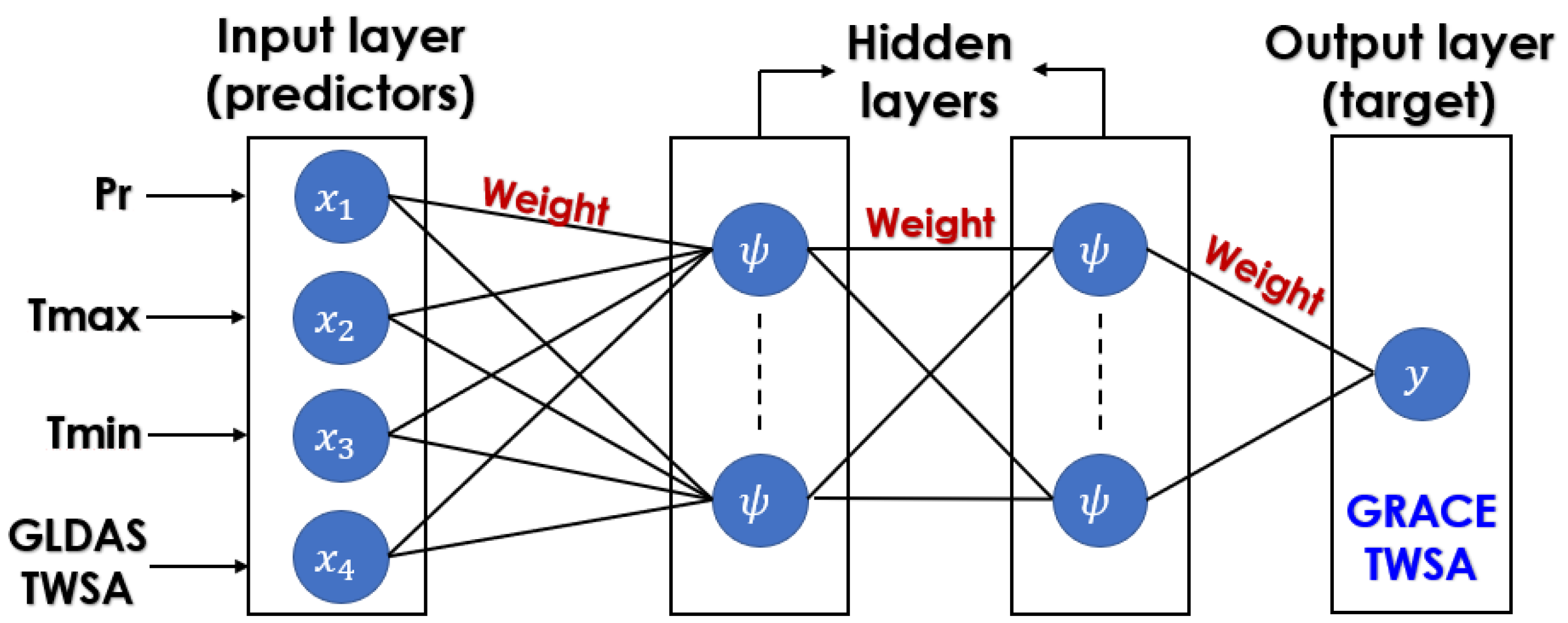
2.3.2. Multilayer Perceptron (MLP)

Artificial neural networks (ANNs) are based on the biological neural network in the brain, which has a billion connected neurons. ANNs have been utilized to imitate the dispersed storage qualities and huge parallel processing of the brain due to developments in information processing [54]. A data processing system called an artificial neural network (ANN) is made up of a densely connected network of neurons, which are basic processing units. By connecting to neurons in the subsequent layer, these neurons are arranged in layers inside the network. The “weight” measures the strength of these connections between two adjacent layers and is comparable to the signal intensity in a biological neural network. The weights of the interconnections are changed throughout the training/learning phase until the inputs yield the desired output. Depending on the training data supplied to the network, various training rules for weight adjustment are necessary to create the desired output [32]. A well-known and frequently used ANN model is the multilayer perceptron (MLP) [32,55]. MLPs have been demonstrated to predict almost any function to any desired accuracy when given enough hidden units and input. This study implemented an MLP model to fill the data gap that exist between the two GRACE missions during 2017 and 2018.

A network of connected nodes or neurons makes up the MLP. The output signals can be changed using a straightforward nonlinear transfer, or activation function, and the neurons are connected by weights [56,57]. Unit step (Heaviside), linear, and logical (sigmoid) functions are the most often employed activation functions. The nodes in the network’s next layer receive the scaled output of a node as an input from the connecting weights. As a result of the information processing direction, the MLP is described as a feed-forward neural network [58].

The output layer of the MLP is followed by one or more hidden layers. One layer’s output feeds into the input of the next layer, etc. The first and last layers of a neural network are input and output, whereas the other levels serve as hidden layers within the network. The weight of each neuronal connection varies. The sigmoid perceptron activation functions are the same for all layers. Depending on the usage, either sigmoid or linear functions are used for the output layer [32]. The structure of an MLP with input, output, and hidden layers is shown in Figure 2.

A backpropagation technique is used in the MLP model, which is considered as a generalization of the least mean squared rule [59]. Backpropagation is a weight-correction approach that propagates errors from the output layer backwards, starting with the previous layer. The variables chosen, the training dataset, and the quantity of hidden layers all affect how well the MLP model performs. The nonlinear function may be detected with less precision if only a few hidden layers are used. Conversely, selecting more hidden layers can cause the training set to be overfitted. As a result, the optimal number of hidden layers for the analysis is determined.

A functional mapping between predictors ‘x’ and the target variable ‘y’ is given by the MLP model as:

$$y=f\left(x\right)+\epsilon$$

(3)

where, $f$ is the mapping and $\epsilon$ is process noise. All of the MLPs created in this study have a single or double hidden layer. An MLP is created by a series of transformations that combine layers one by one. First stage is to develop associations between the input and hidden layers. Let ${\left\{x_i\right\}}_{i=1}^M$ represents $M$ predictors and a hidden layer containing $K$ hidden neurons.

$$a_k={\displaystyle \sum }_{i=1}^M{w}_{ki}^{\left(1\right)}{x}_i+w_{k0}^{\left(1\right)}, k=1,\dots ,K$$

(4)

where, $a_k=$ hidden neuron; ${\left\{w_{ki}^{\left(1\right)}\right\}}_{i=1}^M=$ unknown weights with respect to input neuron; $w_{k0}^{\left(1\right)}=$ bias term; superscript represents the layer number. Next, the above equation is passed through a transfer function in order to produce outputs from hidden neurons.

$$z_k=\psi \left(a_k\right), k=1,\dots ,K$$

(5)

where, $z_k$ represents the output; $\psi$ denotes the transfer function i.e., sigmoid function, which ranges in [0, 1]. Finally, linear transfer functions are used to establish the connection between the hidden and output layers.

$$y_j={\displaystyle \sum }_{k=1}^K{w}_{jk}^{\left(2\right)}{z}_k+w_{j0}^{\left(2\right)}$$

(6)

where, $y_j$ represents the output neuron i.e., model predictions $\left(j=1,\dots ,J\right)$; ${\left\{w_{jk}^{\left(2\right)}\right\}}_{k=1}^K=$ unknown weights of the output layer; $w_{j0}^{\left(2\right)}$ = bias term. Backpropagation techniques are used to solve unknowns in Equations (5) and (6) during the training period in order to acquire the appropriate weights in each layer. For further information regarding multilayer perceptron’s, readers are encouraged to read the following publication [56,59,60,61].

2.3.3. Groundwater Storage from GRACE and GLDAS

The GRACE TWSA is the combination of water storage components present above and below the Earth’s surface, as shown below:

$$TWS{A}_t=GWS{A}_t+SMS{A}_t+CWS{A}_t+SWS{A}_t+SS{A}_t$$

(7)

where TWSA_t, GWSA_t, SMSA_t, CWSA_t, SWSA_t and SSA_t represent terrestrial water storage anomaly, groundwater storage anomaly, soil moisture storage anomaly, canopy water storage anomaly, surface water storage anomaly, and snow water storage anomaly, respectively, at any time t.

For Telangana state, SWSA in the form of reservoir and lake storage is relatively small when compared with GRACE TWSA and $SSA$ is zero for non-snow regions. Then, the above equation becomes:

$$TWS{A}_t=GWS{A}_t+SMS{A}_t+CWS{A}_t$$

(8)

where SMSA and CWSA are obtained from GLDAS Noah model using the following equation:

$$SMS{A}_t=SM{S}_t-\overline{SM{S}_{2004–2009}}$$

(9)

$$CWS{A}_t=CW{S}_t-\overline{CW{S}_{2004–2009}}$$

(10)

where, $SMS{A}_t and CWS{A}_t=$ soil moisture storage and canopy water storage anomalies at time $t$, $SM{S}_t and CW{S}_t=$ soil moisture and canopy water storages at time $t$, $\overline{SM{S}_{2004–2009}}\mathrm{and}\overline{CW{S}_{2004–2009}}=$ average soil moisture and canopy water storages considered with respect to the GRACE base line period (January 2004 to December 2009).

To obtain groundwater storage anomalies (GWSAs), subtract SMSA and CWSA from TWSA, as shown below:

$$GWS{A}_t=TWS{A}_t-SMS{A}_t-CWS{A}_t$$

(11)

2.3.4. Groundwater Storage from Observation Well Measurements

The point groundwater well measurements are converted into groundwater storage anomalies $\left(GWS{A}_{obs}\right)$ and compared with $\left(GWS{A}_{GRACE}\right)$. The procedure to convert groundwater well measurements into GWSA is presented below. For Telangana state, the observation well measurements are considered from 2003–2020.

First, the mean water level depth $\left(\overline{GWL}\right)$ is subtracted from individual seasonal groundwater well measurement $(GW{L}_{groundwater well})$ at all sites to obtain groundwater level anomalies ($\Delta h$).

$$\Delta h=-\left(GW{L}_{groundwater well}-\overline{GWL}\right)$$

(12)

Second, $\Delta h$ values are multiplied by average specific yield ($S_y$) values to obtain observed groundwater storage $(GW{S}_{Obs})$ at each observation well. The average $S_y$ value is considered as 0.022 form [25]:

$$GW{S}_{Obs}=S_y\times \Delta h$$

(13)

Third, the $GW{S}_{Obs}$ are converted to groundwater storage anomalies $(GWS{A}_{Obs})$ with respect to the GRACE base line period (January 2004 to December 2009):

$$GWS{A}_{Obs}=GW{S}_{Obs}-\overline{GW{S}_{2004–2009}}$$

(14)

2.3.5. Processing of Data

Filling the data gap between two GRACE missions was performed with multilayer perceptron’s (MLPs). The MLP model was created using five predictors (Noah TWSA, precipitation, maximum temperature, minimum temperature, and CLSM GWSA) and a predictand (GRACE TWSA). The GLDAS ΔSM and ΔCWS were added to obtain Noah TWSA. The input predictors used for the development of MLP model were considered from 2003 to 2016 (GRACE mission period) and are shown in Figure 3.

The GRACE TWSA and forcing datasets were decomposed into interannual, seasonal, linear trend, and residual parts using the STL method. The de-seasoned (i.e., residual and interannual) parts were reconstructed using the best MLP model for the study region. After the reconstruction, the seasonal component was added back to obtain a complete TWSA series. The STL-decomposed signals for GRACE TWSA, Noah TWSA, precipitation, and CLSM GWSA are shown in Figure 4.

The MLP model was trained using STL-decomposed Noah TWSA, precipitation, maximum temperature, minimum temperature, and CLSM GWSA (predictors) and GRACE TWSA (predictand) datasets from January 2003 to December 2013 (~75% of the samples). The developed MLP model was tested using datasets from January 2014 to December 2016 (~25% of the samples) for the study region. The best MLP model developed using the training dataset was utilized to fill the data gap between the two missions. Additionally, GRACE TWSA was predicted until 2020 and compared with the GRACE FO TWSA dataset. Finally, a continuous time series of TWSA from 2003 to 2020 was generated using the best MLP model. The training and testing period of GRACE TWSA is shown in Figure 5. During the training phase, TWSA displayed an increase in interannual variability, but during the testing period, it decreases (see Figure 5). TWSA increased because of an increase in precipitation anomalies in South India between 2003 and 2013. [15,62]. Because of the unpredictability in precipitation over the testing period, decreasing trends in TWSA were seen. The severe drought in South India from 2015 to 2018 resulted in precipitation shortfalls of more than 40% and a decline in TWSA [62].

TWSA was converted into GWSA GWSA_GRACE using GLDAS Noah SMSA and CWSA values from 2003 to 2020. The obtained GWSA_GRACE was converted to seasonal values. Four seasons were taken into consideration, as provided by the Central Groundwater Board. The point observation well measurements were converted to groundwater storage anomalies (GWSA_obs). Then, the seasonal GWSA_GRACE values were validated with seasonal (GWSA_obs) obtained from point observation well data. A statistical metric named Pearson’s correlation was used to evaluate the correlation between GWSA_GRACE with (GWSA_obs) for Telangana state.

3. Results and Discussion

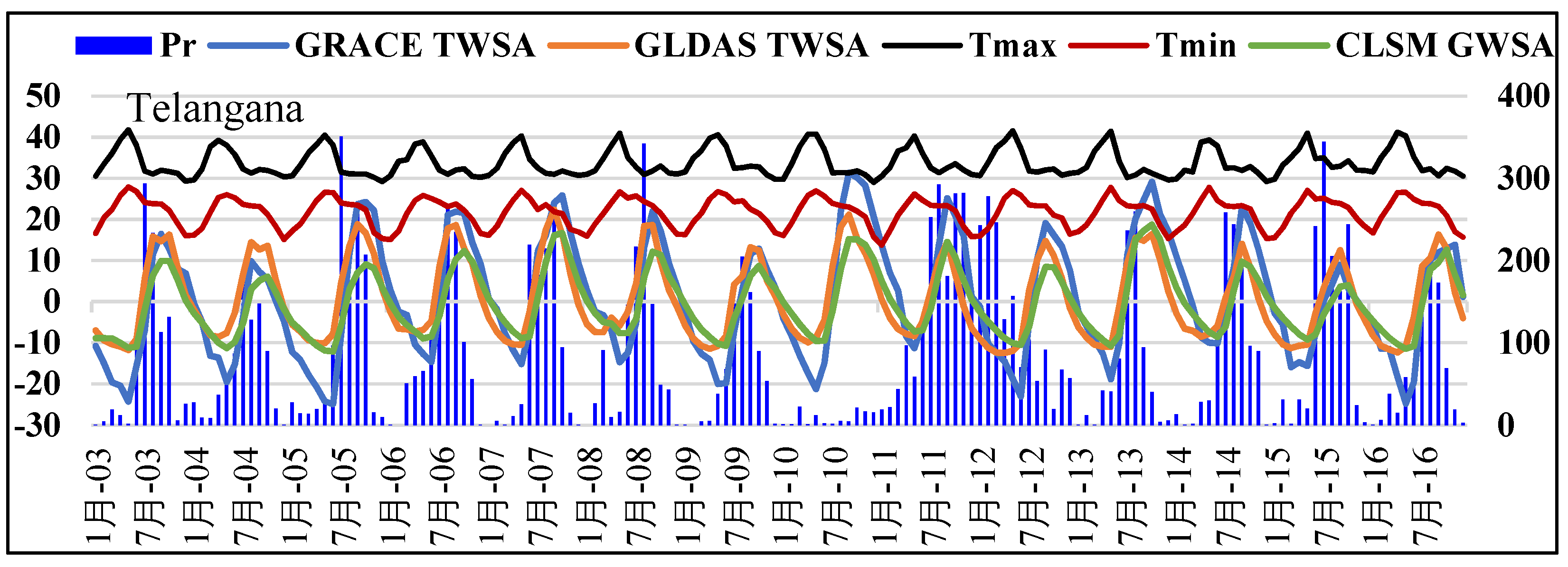
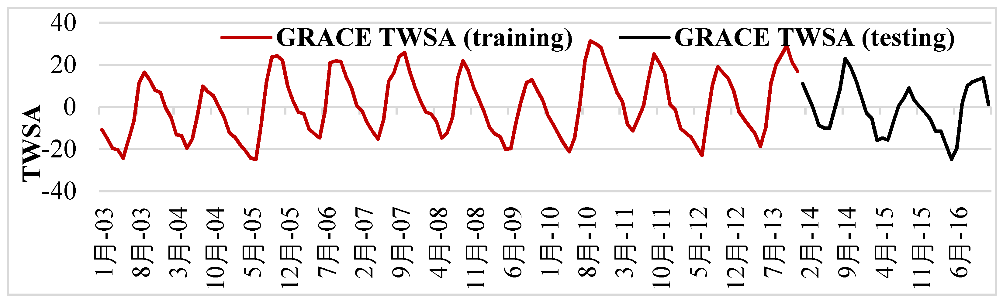
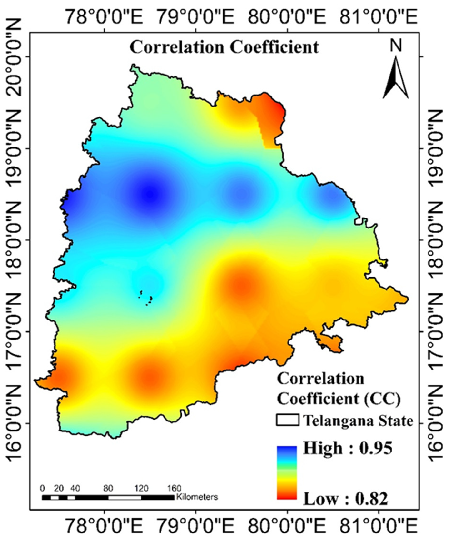
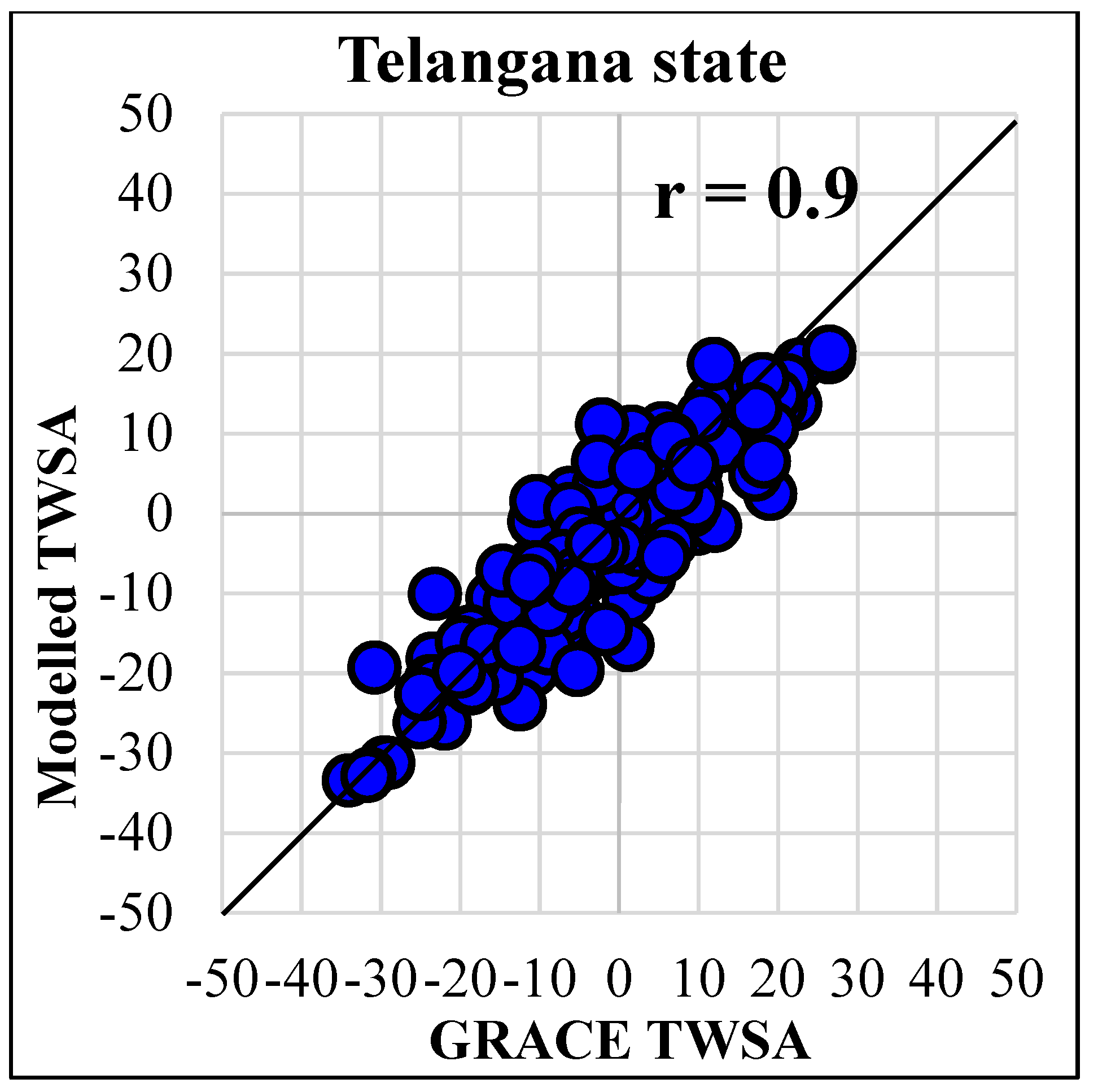
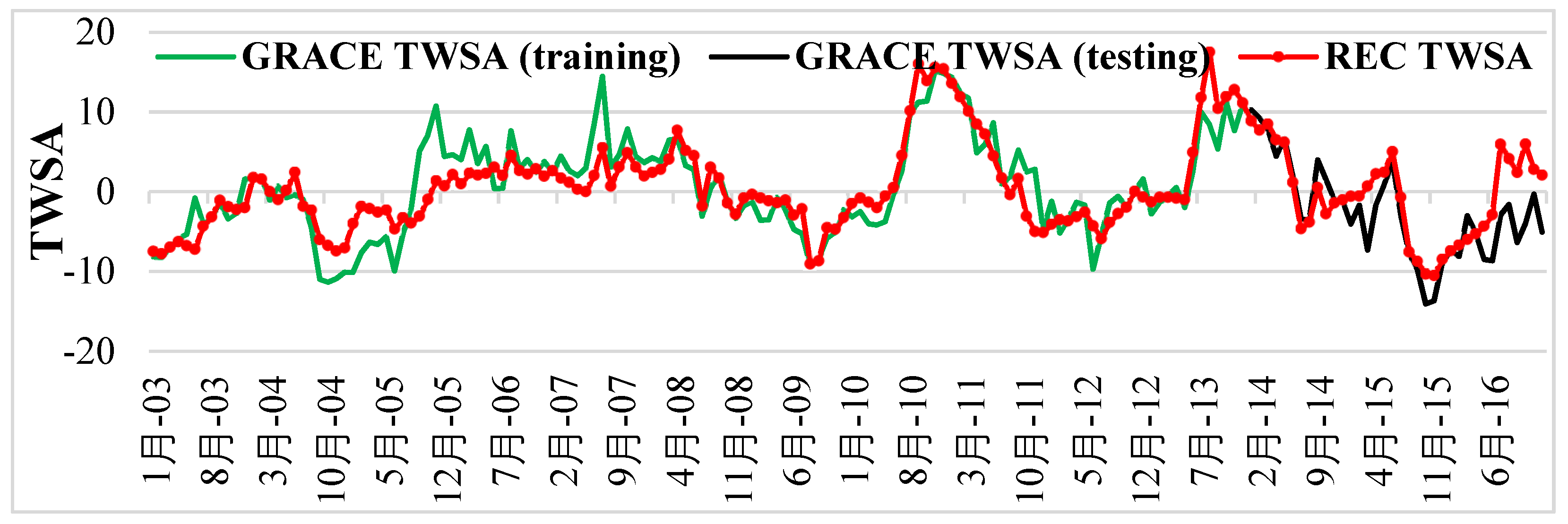
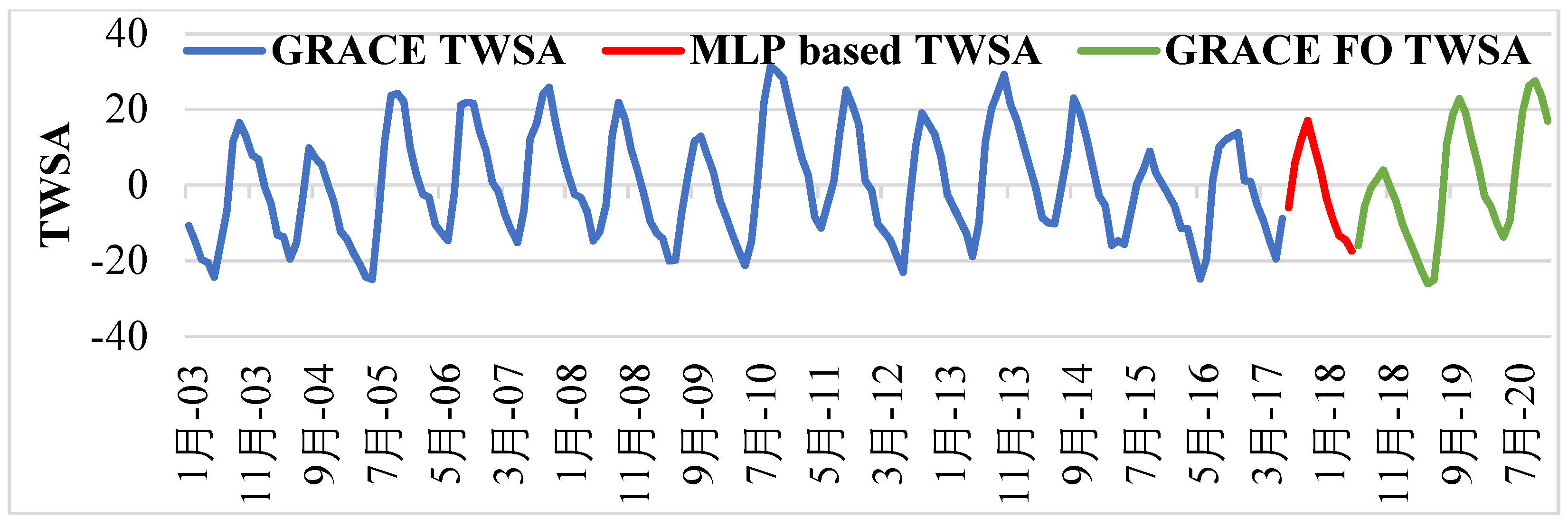
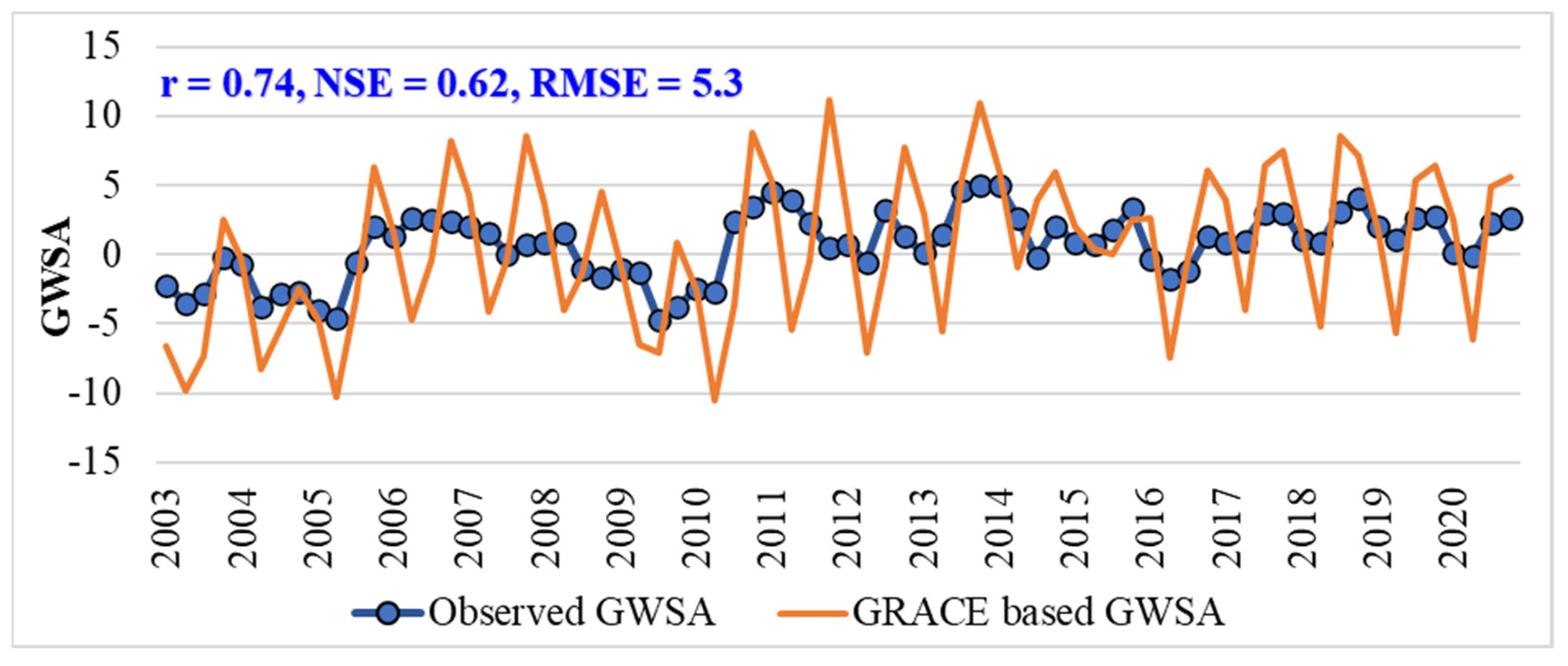
3.1. Model Evaluation at Regional Scale

The regional-scale investigation enabled a detailed assessment of several models for GRACE TWSA prediction between 2017 and 2018. The de-seasoned (interannual and residual) predictor and predictand datasets were utilized in training the neural network. We initially set the training method (Levenberg–Marquardt algorithm), learning rate (0.05), epochs (1000), and cost function using the trial-and-error method (mean squared error, MSE). When the MSE was less than 0.001 or when there had been 1000 iterations, the training was stopped. The final model parameters and model prediction performance were recorded after the termination criteria were satisfied. The number of neurons in each hidden layer varied from 3 to 15, and the range of hidden layers was set at 1 to 2. The most popular functions in the hydrology field, “tansig,” “logsig,” and “purelin,” were utilized as the activation functions.

The developed MLP model achieved high accuracy during the training and testing period. In this section, we analyze the magnitudes and geographical distributions of commonly used measures, namely, the correlation coefficient (r) generated by the observed and simulated GRACE TWSA throughout the testing period. The majority of Telangana state experienced r values of more than 0.8, as shown in Figure 6. During the test period, the modeled TWSA and GRACE TWSA were compared to more intuitively assess the reconstructed GRACE TWSA (Figure 7). With a correlation coefficient of 0.96, Telangana state’s GRACE TWSA and MLP-simulated TWSA showed a strong association. The trained leading MLP model was used for the prediction of GRACE TWSA from 2017 to 2018.

The best MLP model was developed using the decomposed predictors, and, using this best MLP model, the TWSA was reconstructed from 2003 to 2017 and projected until 2020. Figure 8 displays the decomposed original TWSA (training and testing periods) and the MLP model-developed TWSA (red dotted line) between 2003 and 2017. The figure demonstrates clearly that the model-based TWSA and the original TWSA matched each other. The best MLP model was used to fill the data gap between the two missions (2017 to 2018). The TWSA series was then extended through 2020 using the same model, and compared with the GRACE FO TWSA. After reconstructing the de-seasoned GRACE TWSA, the seasonal component was re-added to retrieve the entire TWSA series from 2003 to 2020 (see Figure 9). Figure 9 shows the GRACE TWSA from 2003 to 2020 for Telangana state, comprising observed TWSA from 2003 to 2017 (blue line), the MLP model-based TWSA from 2017 to 2018 (red line), and the GRACE FO TWSA from 2018 to 2020 (green line). Figure 10 shows the GRACE FO TWSA from 2018 to 2020 and the predicted TWSA using the MLP model from 2017 to 2020. The figure clearly shows that there is good agreement between the GRACE FO TWSA and the MLP-simulated TWSA, with a correlation coefficient of 0.93. Further GWSA evaluation and comparison with observation well-based GWSA was carried out using the TWSA series from 2003 to 2020.

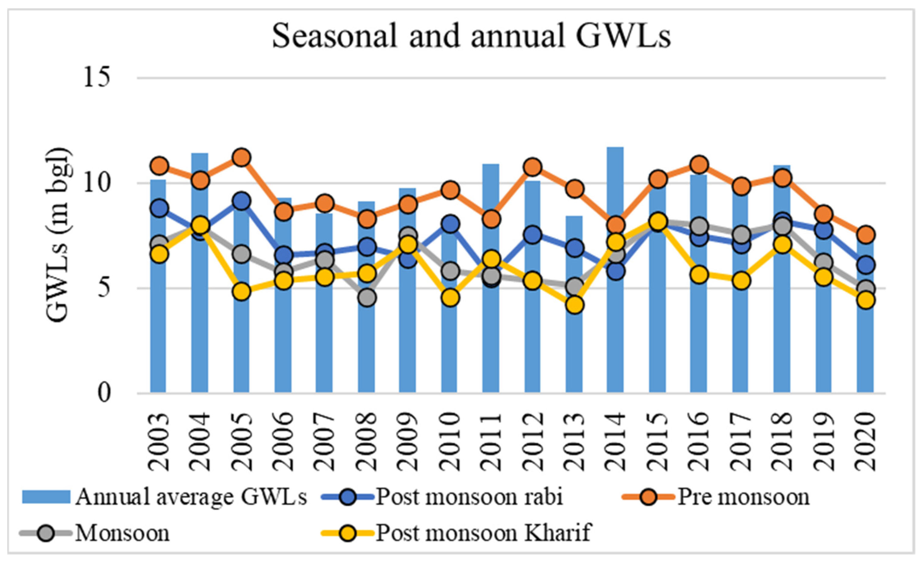
3.2. Seasonal and Annual Groundwater Level Measurements

Figure 11 displays the seasonal and annual GWLs for Telangana state from 2003 to 2020 that were acquired from the CGWB. Since the groundwater was accessible within 5 m of the ground level, there were good groundwater levels in the post-monsoon kharif season. This is due to the fact that availability of surface water is greater in the post-monsoon season (October), in the form of reservoirs, lakes, and ponds, which are utilized for irrigation and domestic purposes. Additionally, rainfall occurring during the monsoon season will add to the groundwater.

Due to inadequate surface water storage, a large amount of groundwater is used in the pre-monsoon (May) period. Since May is the hottest month of the year, there is less surface water availability and more groundwater usage. As a result, groundwater levels are typically 10 meters below ground level (mbgl) in the pre-monsoon season, as shown in Figure 11. Groundwater levels during the monsoon season (Aug) ranged from 5 to 7 (mbgl). Surface water is more readily available during this season because most parts of the nation experience rain during this time. As there is enough surface water available, less groundwater is used for irrigation and other purposes. Moreover, an increase in GWLs can be observed in this season. During the post-monsoon rabi season (Jan), groundwater levels were at a depth of 6 to 8 mbgl. The groundwater demand during the post-monsoon rabi season was moderate compared to that of the remaining seasons. The results are in line with the earlier trend analysis of seasonal groundwater levels for part of Telangana state [63,64].

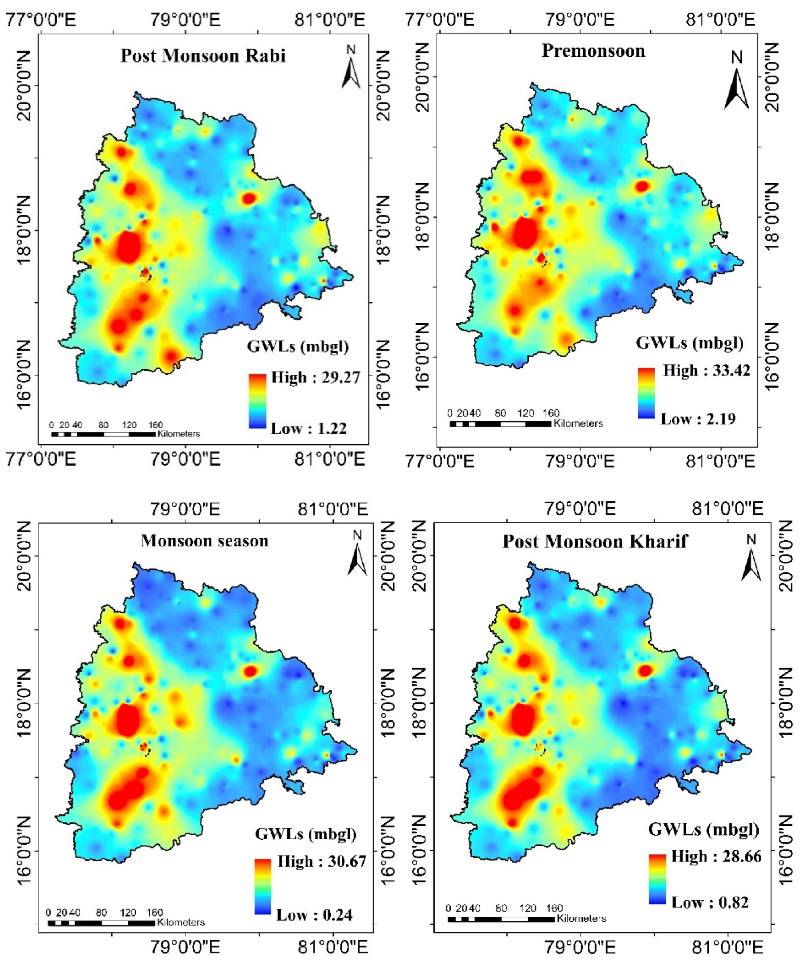
3.3. Spatial Analysis of Seasonal Groundwater Levels from 2003 to 2020

The seasonal groundwater levels (GWLs) obtained from CGWB for the period 2003–2020 were averaged over Telangana state and are presented in Figure 12. The pre-monsoon season (May) experienced the highest reduction in GWLs compared to the other seasons. In India, groundwater usage for irrigation, domestic, and industrial purposes is greatest in May because it is the hottest month of the year. Additionally, since is less surface water throughout the summer, the majority of India depends on groundwater during the summer season. The central and western regions of the state experienced the lowest groundwater level during the pre-monsoon season, which was approximately 33 mbgl (meters below ground level).

Followed by the pre-monsoon season, the monsoon season experienced a reduction in groundwater levels in the western and central parts of the state. Since 75% of India’s rain falls during the monsoon season, the majority of irrigation is carried out during this period. As a result, a significant amount of water is used for irrigation throughout this season. As the rainfall is unevenly distributed throughout the country, most irrigation is carried out using groundwater [15,60]. Therefore, a reduction in groundwater levels can be observed during the monsoon season.

The post-monsoon rabi and kharif seasons also experienced lower groundwater levels in the central and western parts of the state. For the post-monsoon rabi season, the lowest GWL was recorded as 29 mbgl, whereas for the post-monsoon kharif season, this was 28 mbgl. Telangana is one of the large producers of paddy rice, and more than 50% of its population depends on irrigation; therefore, groundwater usage is greater in all seasons. As a result, considerable measures should be taken to reduce the over-exploitation of groundwater storage in Telangana state.

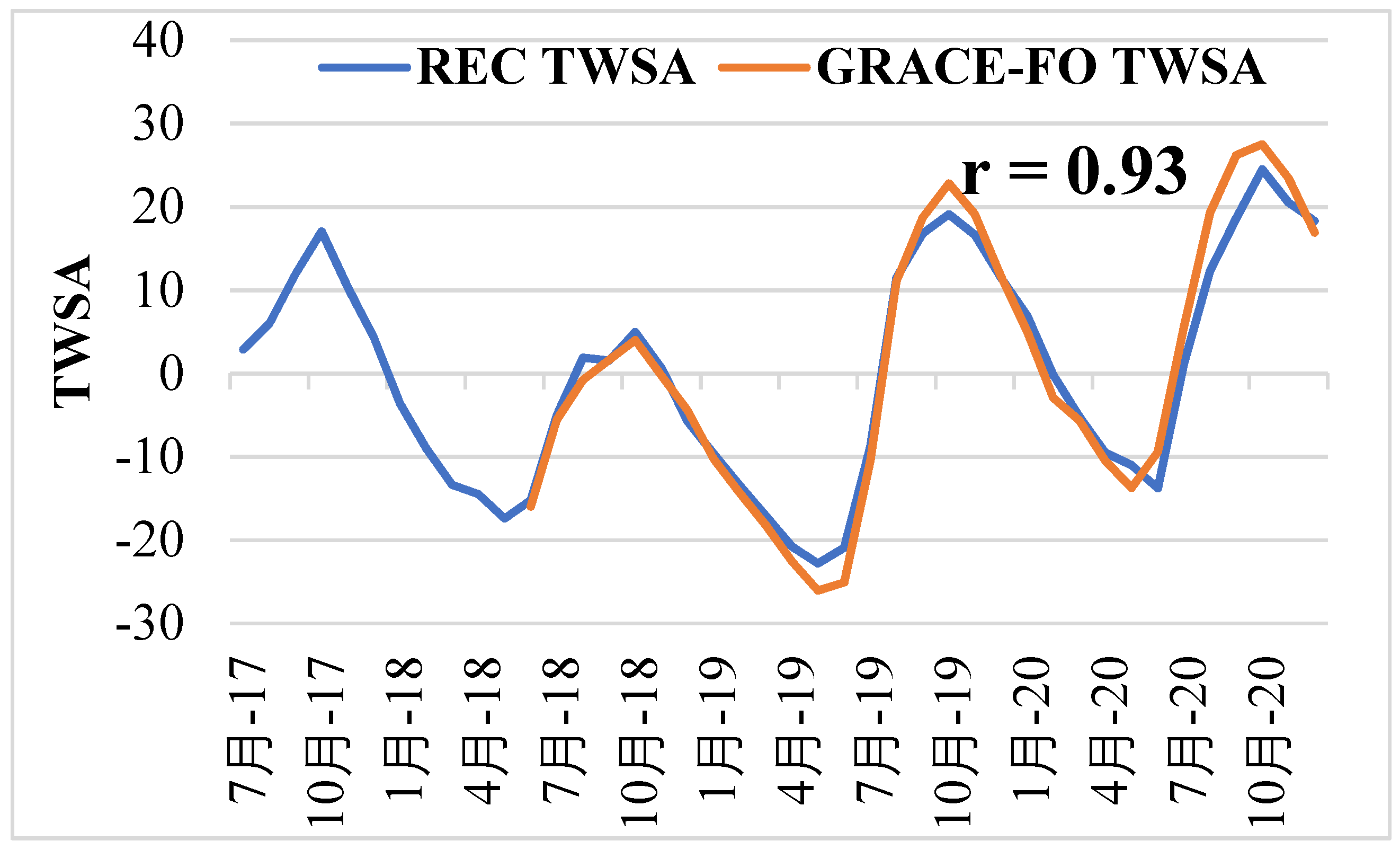
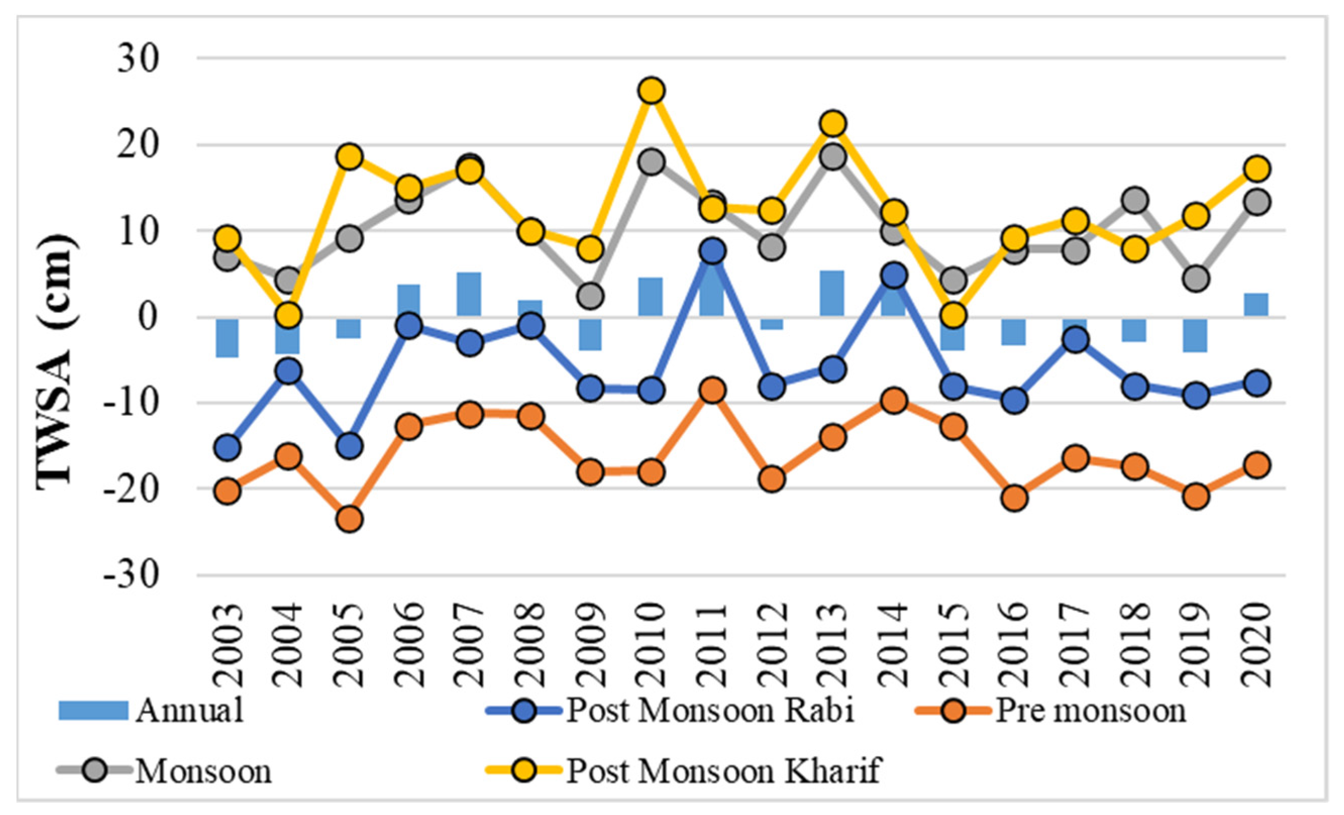
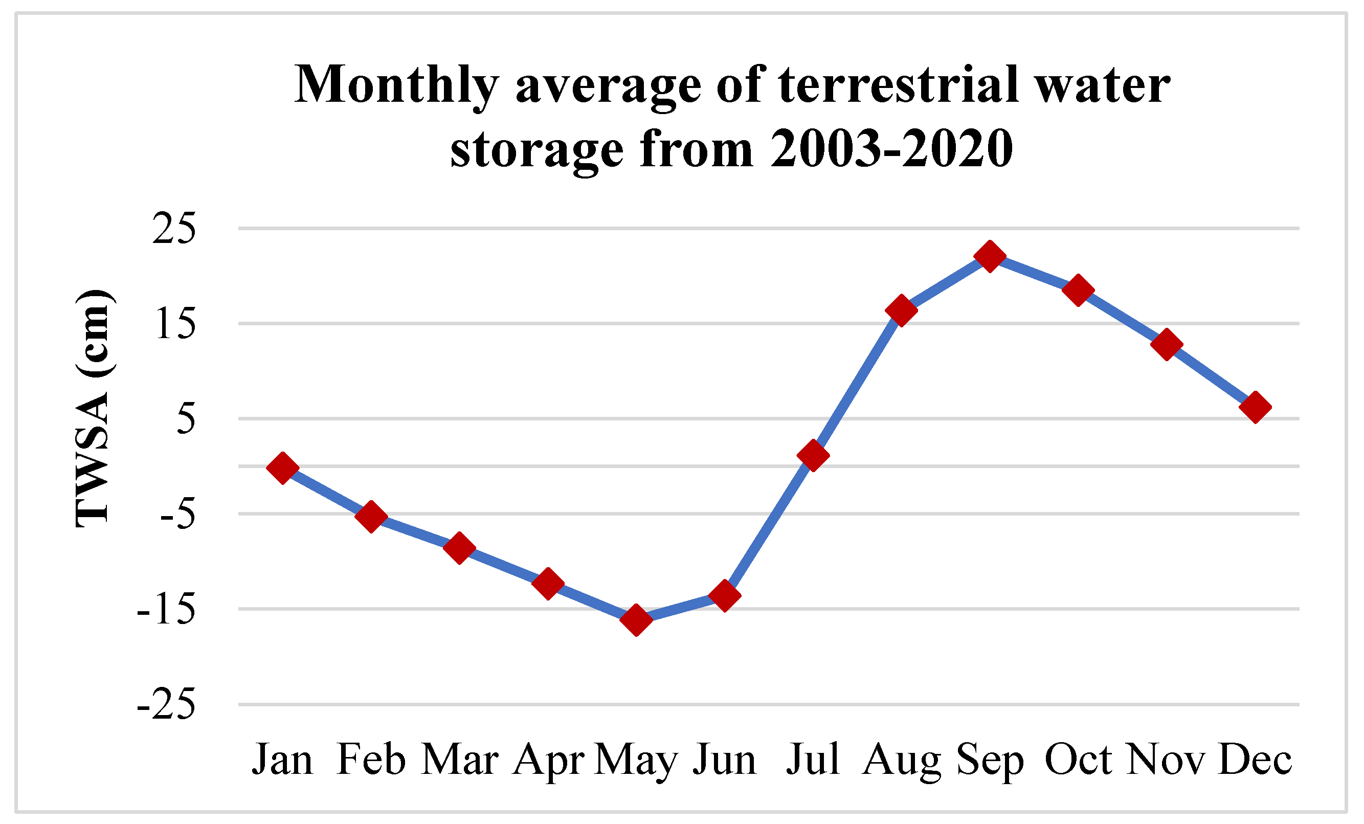
3.4. Seasonal and Annual Terrestrial Water Storage Anomalies

The GRACE TWSAs were calculated for four seasons, as for the observation well data, and the variations are presented in Figure 13. Figure 13 represents seasonal and annual TWSAs for Telangana state from 2003 to 2020. The monsoon and post-monsoon kharif seasons exhibited positive TWSAs, whereas post-monsoon rabi and pre-monsoon seasons displayed negative trends. The lowest TWSA values were observed in pre-monsoon seasons. The annual values varied from year to year, and negative TWSA values were observed in the years 2003, 2004, 2005, 2009, 2012, 2015, and 2016–19, leading to severe droughts in 2003–2005, 2009, 2015–2016, and 2018–2019. Overall, at both the annual and seasonal scales, TWSA showed a downward trend from the beginning of the 21st century in Telangana state.

Figure 14 represents the monthly average of TWSA values from 2003 to 2020. The TWSAs decreased from January to June and increased from July to December. The highest negative and positive TWSAs were observed in the months of May and September, respectively. In the pre-monsoon season, due to unavailability of surface water resources, excess usage of groundwater storage can be observed in Figure 13; the opposite pattern can be observed in the case of the monsoon season. Overall, the TWSAs exhibit decreasing trends for the first half of the calendar year, and an increasing trend for the second half the year.

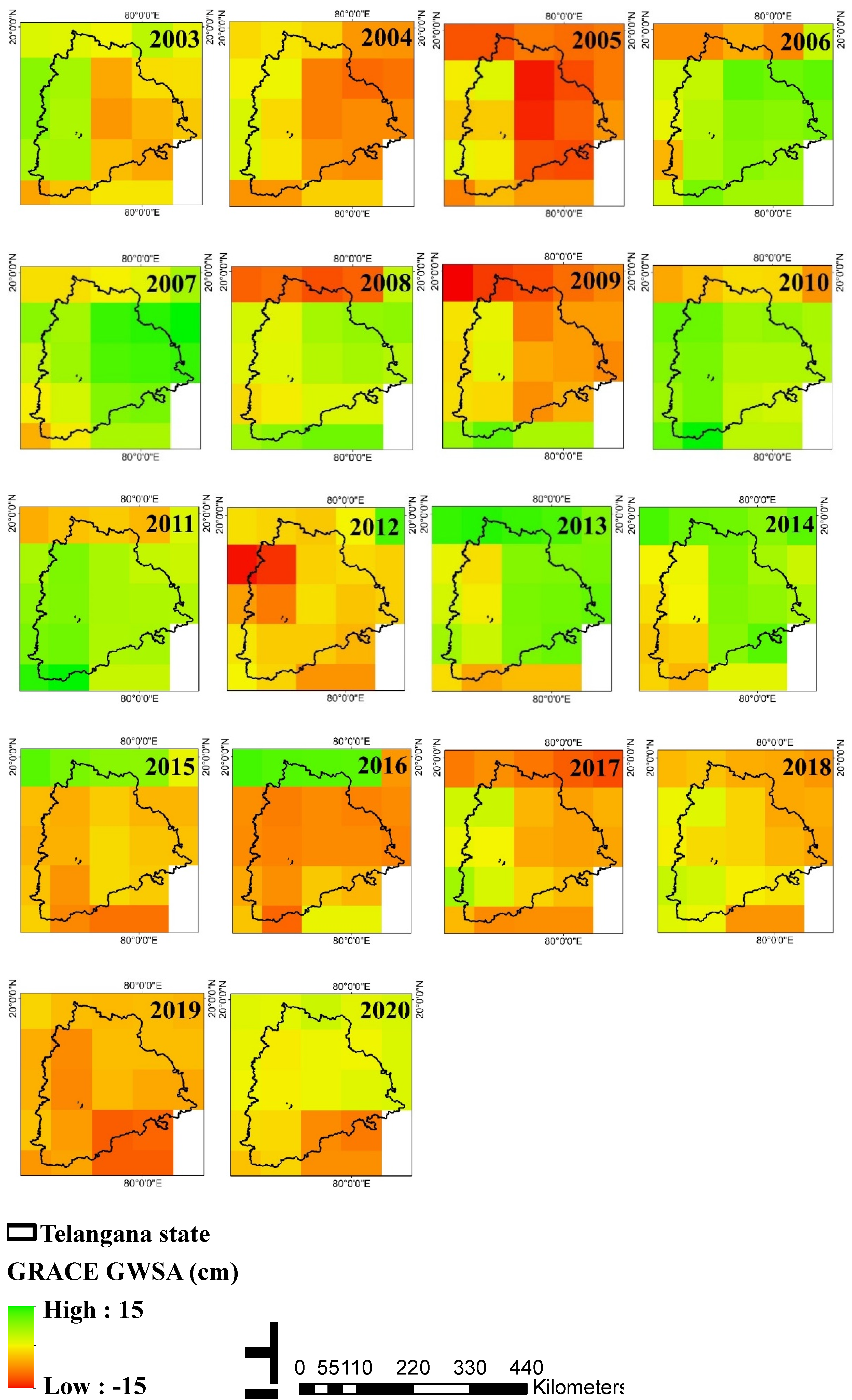
3.5. Spatial Analysis of Annual GRACE Groundwater Storage Anomalies

The monthly GWSA values from GRACE were converted to average annual values, and spatial maps were derived for Telangana state from 2003 to 2020. The annual GWSA estimates demonstrated the emergence of intense groundwater depletion zones in the state, as shown in Figure 15. Telangana state showed decreasing GWSA in the years 2005, 2009, and 2015–2019. Positive GWSAs were observed in the years 2006, 2007, 2010, 2011, 2013, and 2014. A negative GWSA represents a decrease in the water storage and the occurrence of droughts.

The $GWS{A}_{GRACE}$ findings are in line with those of earlier research on drought occurrences carried out in Southern India [9,16,25,60,62,65]. According to [9,60], Godavari and Krishna basins suffered droughts during 2003–2005, 2009–2010, 2012–2013, and 2015–2016. The present study also exhibited similar results as experienced by the state in terms of decreasing GWSA during these years. The 2015 drought had an impact on crop output and water availability in Central and Southern regions [66,67]. The 2015–2016 drought affected a significant portion of South India, and reduced reservoir storage and hydropower output. Around 330 million people in ten states of India, particularly in Southern India, were affected by the 2015–2016 drought, which significantly reduced groundwater supplies [68]. According to [62], Southern India (Telangana and Andhra Pradesh) experienced a severe drought and a worsening water constraint between 2016 and 2018, which was in line with the decreased GWSA in Telangana state, as shown in Figure 15. Indicating that GRACE TWSA can be utilized to assess research linked to drought, GRACE GWSA fluctuations in the current study are compatible with past records of drought occurrences in the Southern region of India, especially Telangana and Andhra Pradesh states.

3.6. Comparison of $\mathit{GWS}{\mathit{A}}_{\mathit{GRACE}}$ with $\mathit{GWS}{\mathit{A}}_{\mathit{OBS}}$ at a Seasonal Scale

The GRACE TWSA was converted into $GWS{A}_{GRACE}$ and validated with GWSA obtained from observation well measurements $GWS{A}_{OBS}$. Pearson’s correlation coefficient (r) between $GWS{A}_{GRACE}$ and $GWS{A}_{OBS}$ is shown in Figure 16. The x-axis represents four seasons for each year from 2003 to 2020. A significant correlation is observed between $GWS{A}_{GRACE}$ and $GWS{A}_{OBS}$, with r = 0.74 for Telangana state. The coefficient values provide vital information about the magnitude of the closeness in the data. The RMSE value between seasonal $GWS{A}_{GRACE}$ and $GWS{A}_{OBS}$ displayed the closest relationship, with RMSE = 5.3. The NSE value displayed a good relationship, with NSE = 0.62. Figure 16 shows an increasing trend in GWSAs during 2005–2007 and 2010–2012. Subsequently, a decreasing trend in GWSAs was observed during 2008–2010 and 2014–2016 in Telangana state.

For the study region, a significant seasonal relationship between $GWS{A}_{GRACE}$ and $GWS{A}_{OBS}$ can be seen. From 2011 to 2020, the seasonality pattern was correctly predicted by $GWS{A}_{GRACE}$, although from 2003 to 2010, the pattern was somewhat underestimated or overestimated. The majority of precipitation falls in Telangana state throughout the monsoon season (June to September) [69]. As a result, the pre-monsoon season saw the lowest GWS values, while the monsoon season saw the highest GWS values. Seasonality in groundwater storage is influenced by climate variables such as precipitation and evapotranspiration, particularly in regions with shallow groundwater tables [70]. Because Telangana has a distinct monsoon season, the period of June to September sees the majority (>74%) of the state’s yearly precipitation. The water from surface water bodies and canals has been used to model additional groundwater influx elements [71]. Furthermore, irrigation-related pumping has dramatically decreased the groundwater storage in the Telangana state [72].

4. Conclusions

In this study, firstly, we aimed to bridge the data gap between GRACE and GRACE FO missions using multilayer perceptron’s to obtain a continuous dataset from 2003 to 2020 for Telangana state, India. Secondly, the GRACE TWSA data were analyzed at spatial and temporal time scales, and converted to seasonal GWSA values using GLDAS land surface model parameters. Thirdly, the observation well measurements were analyzed and converted to GWSA values at a seasonal scale. Finally, $GWS{A}_{GRACE}$ data were validated with $GWS{A}_{obs}$ using Pearson’s correlation analysis from 2003 to 2020 for Telangana state. The $GWS{A}_{GRACE}$ matched well with the ground-based estimates for the study region, which is climatologically and hydro-geologically varied.

The findings show that the MLP model performed reasonably well in predicting GRACE TWSA from 2017 to 2020. A correlation of r = 0.96 was observed between the modeled TWSA and GRACE TWSA for the test period. Moreover, good agreement was observed between the GRACE FO TWSA and the MLP-simulated TWSA between 2018 and 2020, with a correlation coefficient of 0.93. Overall, the developed MLP models can be used to fill the data gap between two missions. The predicted GRACE TWSA dataset can help to obtain a continuous series from 2003 to the present, which can be used to analyze the long-term climate-related applications in any region.

An increase in GWLs was observed in the post-monsoon season and decreasing GWLs were observed in the monsoon season. Annually decreasing GWLs were observed from 2017 to 2020 due to overexploitation of groundwater for irrigation purposes. Therefore, considerable measures should be taken to reduce the over-exploitation of groundwater storage in Telangana state. Seasonal $GWS{A}_{GRACE}$ correlated well with GWSA_obs from 2003 to 2020 for the study region. GWSA_GRACE exhibited strong seasonality, like that of GWSA_obs The GWSA_GRACE estimates correlated well with GWSA_obs, with r = 0.74.

The limitation of CLSM groundwater storage is that it simulates only shallow groundwater storage. Moreover, the effect of surface water storage was also not considered in this study. Overall, the MLP technique is effective in filling the TWSA data gap between the GRACE and GRACE FO missions. The satellite-based GRACE data can be used to assess terrestrial water storage, in addition to groundwater storage globally where there is a lack of observed groundwater level data. Based on the results of this work, the methodology can be adopted to predict and reconstruct TWSA data at regional and global scales with similar meteorological, hydrogeologic, and groundwater withdrawal conditions.

References

1. Mukherjee, A.; Saha, D.; Harvey, C.F.; Taylor, R.G.; Ahmed, K.M.; Bhanja, S.N. Groundwater systems of the Indian Sub-Continent. J. Hydrol. Reg. Stud. 2015, 4, 1–14. [Google Scholar] [CrossRef] [Green Version]
2. Asoka, A.; Gleeson, T.; Wada, Y.; Mishra, V. Relative contribution of monsoon precipitation and pumping to changes in groundwater storage in India. Nat. Geosci. 2017, 10, 109–117. [Google Scholar] [CrossRef] [Green Version]
3. Rodell, M.; Famiglietti, J.S.; Wiese, D.N.; Reager, J.T.; Beaudoing, H.K.; Landerer, F.W.; Lo, M.-H. Emerging trends in global freshwater availability. Nature 2018, 557, 651–659. [Google Scholar] [CrossRef] [PubMed]
4. Siebert, S.; Kummu, M.; Porkka, M.; Döll, P.; Ramankutty, N.; Scanlon, B.R. A global data set of the extent of irrigated land from 1900 to 2005. Hydrol. Earth Syst. Sci. 2015, 19, 1521–1545. [Google Scholar] [CrossRef] [Green Version]
5. Famiglietti, J.S.; Rodell, M. Water in the balance. Science 2013, 340, 1300–1301. [Google Scholar] [CrossRef]
6. Food and Agriculture Organization of the United Nations. FAO Statistical Yearbook 2013: World Food and Agriculture; Food and Agriculture Organization of the United Nations: Rome, Italy, 2013; 289p. [Google Scholar]
7. Pahuja, S.; Tovey, C.; Foster, S.; Garduno, H. Deep Wells and Prudence: Towards Pragmatic Action for Addressing Groundwater Overexploitation in India; World Bank: Washington, DC, USA, 2010. [Google Scholar]
8. Satish Kumar, K.; AnandRaj, P.; Sreelatha, K.; Sridhar, V. Regional analysis of drought severity-duration-frequency and severity-area-frequency curves in the Godavari River Basin, India. Int. J. Climatol. 2021, 41, 5481–5501. [Google Scholar] [CrossRef]
9. Kumar, K.S.; AnandRaj, P.; Sreelatha, K.; Bisht, D.; Sridhar, V. Monthly and Seasonal Drought Characterization Using GRACE-Based Groundwater Drought Index and Its Link to Teleconnections across South Indian River Basins. Climate 2021, 9, 56. [Google Scholar] [CrossRef]
10. Dixit, S.; Jayakumar, K.V. Spatio-temporal analysis of copula-based probabilistic multivariate drought index using CMIP6 model. Int. J. Clim. 2022, 42, 4333–4350. [Google Scholar] [CrossRef]
11. Central Ground Water Board (CGWB). Ground Water Year Book–Telangana State 2020–2021; G.o.I. Ministry of Water Resources: New Delhi, India, 2020; p. 3. [Google Scholar]
12. Zaveri, E.; Grogan, D.S.; Fisher-Vanden, K.; Frolking, S.; Lammers, R.B.; Wrenn, D.H.; Prusevich, A.; Nicholas, R.E. Invisible water, visible impact: Groundwater use and Indian agriculture under climate change. Environ. Res. Lett. 2016, 11, 084005. [Google Scholar] [CrossRef] [Green Version]
13. Ministry of Agriculture (MoA), Government of India. State of Indian Agriculture 2011–2012; Ministry of Agriculture (MoA), Government of India: New Delhi, India, 2012. [Google Scholar]
14. Rodell, M.; Velicogna, I.; Famiglietti, J.S. Satellite-based estimates of groundwater depletion in India. Nature 2009, 460, 999–1002. [Google Scholar] [CrossRef]
15. Kumar, K.S.; Rathnam, E.V.; Sridhar, V. Tracking seasonal and monthly drought with GRACE-based terrestrial water storage assessments over major river basins in South India. Sci. Total Environ. 2021, 763, 142994. [Google Scholar] [CrossRef] [PubMed]
16. Soni, A.; Syed, T.H. Diagnosing Land Water Storage Variations in Major Indian River Basins using GRACE observations. Glob. Planet. Change 2015, 133, 263–271. [Google Scholar] [CrossRef]
17. Rodell, M.; Chen, J.; Kato, H.; Famiglietti, J.S.; Nigro, J.; Wilson, C.R. Estimating groundwater storage changes in the Mississippi River basin (USA) using GRACE. Hydrogeol. J. 2007, 15, 159–166. [Google Scholar] [CrossRef] [Green Version]
18. Flechtner, F. AOD1B Product Description Document for Product Releases 01 to 04 (Rev. 3.1, April 13, 2007); GRACE Project Document: Potsdam, Germany, 2007; pp. 327–750. [Google Scholar]
19. Landerer, F.W.; Swenson, S.C. Accuracy of scaled GRACE terrestrial water storage estimates. Water Resour. Res. 2012, 48, 1–11. [Google Scholar] [CrossRef]
20. Watkins, M.M.; Wiese, D.N.; Yuan, D.-N.; Boening, C.; Landerer, F.W. Improved methods for observing Earth’s time variable mass distribution with GRACE using spherical cap mascons. J. Geophys. Res. Solid Earth 2015, 120, 2648–2671. [Google Scholar] [CrossRef]
21. Wiese, D.N.; Landerer, F.W.; Watkins, M.M. Quantifying and reducing leakage errors in the JPL RL05M GRACE mascon solution. Water Resour. Res. 2016, 52, 7490–7502. [Google Scholar] [CrossRef]
22. Zhang, X.; Li, J.; Dong, Q.; Wang, Z.; Zhang, H.; Liu, X. Bridging the gap between GRACE and GRACE-FO using a hydrological model. Sci. Total Environ. 2022, 822, 153659. [Google Scholar] [CrossRef]
23. Zhang, B.; Yao, Y.; He, Y. Bridging the data gap between GRACE and GRACE-FO using artificial neural network in Greenland. J. Hydrol. 2022, 608, 127614. [Google Scholar] [CrossRef]
24. Li, F.; Kusche, J.; Chao, N.; Wang, Z.; Löcher, A. Long-Term (1979-Present) Total Water Storage Anomalies Over the Global Land Derived by Reconstructing GRACE Data. Geophys. Res. Lett. 2021, 48. [Google Scholar] [CrossRef]
25. Bhanja, S.N.; Mukherjee, A.; Saha, D.; Velicogna, I.; Famiglietti, J.S. Validation of GRACE based groundwater storage anomaly using in-situ groundwater level measurements in India. J. Hydrol. 2016, 543, 729–738. [Google Scholar] [CrossRef]
26. Vissa, N.K.; Anandh, P.C.; Behera, M.M.; Mishra, S. ENSO-induced groundwater changes in India derived from GRACE and GLDAS. J. Earth Syst. Sci. 2019, 128, 115. [Google Scholar] [CrossRef] [Green Version]
27. Verma, K.; Katpatal, Y.B. Groundwater Monitoring Using GRACE and GLDAS Data after Downscaling Within Basaltic Aquifer System. Groundwater 2020, 58, 143–151. [Google Scholar] [CrossRef] [PubMed]
28. Chanu, C.S.; Munagapati, H.; Tiwari, V.M.; Kumar, A.; Elango, L. Use of GRACE time-series data for estimating groundwater storage at small scale. J. Earth Syst. Sci. 2020, 129, 215. [Google Scholar] [CrossRef]
29. Kinouchi, T. Synergetic application of GRACE gravity data, global hydrological model, and in-situ observations to quantify water storage dynamics over Peninsular India during 2002–2017. J. Hydrol. 2021, 596, 126069. [Google Scholar]
30. Girotto, M.; De Lannoy, G.J.M.; Reichle, R.H.; Rodell, M.; Draper, C.; Bhanja, S.N.; Mukherjee, A. Benefits and pitfalls of GRACE data assimilation: A case study of terrestrial water storage depletion in India. Geophys. Res. Lett. 2017, 44, 4107–4115. [Google Scholar] [CrossRef] [PubMed] [Green Version]
31. Hamshaw, S.D.; Dewoolkar, M.M.; Schroth, A.W.; Wemple, B.C.; Rizzo, D.M. A New Machine-Learning Approach for Classifying Hysteresis in Suspended-Sediment Discharge Relationships Using High-Frequency Monitoring Data. Water Resour. Res. 2018, 54, 4040–4058. [Google Scholar] [CrossRef]
32. Long, D.; Shen, Y.; Sun, A.; Hong, Y.; Longuevergne, L.; Yang, Y.; Li, B.; Chen, L. Drought and flood monitoring for a large karst plateau in Southwest China using extended GRACE data. Remote Sens. Environ. 2014, 155, 145–160. [Google Scholar] [CrossRef]
33. Sun, A.Y.; Scanlon, B.R.; Zhang, Z.; Walling, D.; Bhanja, S.N.; Mukherjee, A.; Zhong, Z. Combining Physically Based Modeling and Deep Learning for Fusing GRACE Satellite Data: Can We Learn From Mismatch? Water Resour. Res. 2019, 55, 1179–1195. [Google Scholar] [CrossRef] [Green Version]
34. Li, F.; Kusche, J.; Rietbroek, R.; Wang, Z.; Forootan, E.; Schulze, K.; Lück, C. Comparison of Data-Driven Techniques to Reconstruct (1992–2002) and Predict (2017–2018) GRACE-Like Gridded Total Water Storage Changes Using Climate Inputs. Water Resour. Res. 2020, 56. [Google Scholar] [CrossRef] [Green Version]
35. Sun, Z.; Long, D.; Yang, W.; Li, X.; Pan, Y. Reconstruction of GRACE Data on Changes in Total Water Storage Over the Global Land Surface and 60 Basins. Water Resour. Res. 2020, 56. [Google Scholar] [CrossRef]
36. Osman, A.I.A.; Ahmed, A.N.; Chow, M.F.; Huang, Y.F.; El-Shafie, A. Extreme gradient boosting (Xgboost) model to predict the groundwater levels in Selangor Malaysia. Ain Shams Eng. J. 2021, 12, 1545–1556. [Google Scholar] [CrossRef]
37. Afan, H.A.; Osman, A.I.A.; Essam, Y.; Ahmed, A.N.; Huang, Y.F.; Kisi, O.; Sherif, M.; Sefelnasr, A.; Chau, K.-W.; El-Shafie, A. Modeling the fluctuations of groundwater level by employing ensemble deep learning techniques. Eng. Appl. Comput. Fluid Mech. 2021, 15, 1420–1439. [Google Scholar] [CrossRef]
38. Banadkooki, F.B.; Ehteram, M.; Ahmed, A.N.; Teo, F.Y.; Fai, C.M.; Afan, H.A.; Sapitang, M.; El-Shafie, A. Enhancement of Groundwater-Level Prediction Using an Integrated Machine Learning Model Optimized by Whale Algorithm. Nonrenew. Resour. 2020, 29, 3233–3252. [Google Scholar] [CrossRef]
39. Voss, K.A.; Famiglietti, J.S.; Lo, M.-H.; De Linage, C.; Rodell, M.; Swenson, S.C. Groundwater depletion in the Middle East from GRACE with implications for transboundary water management in the Tigris-Euphrates-Western Iran region. Water Resour. Res. 2013, 49, 904–914. [Google Scholar] [CrossRef] [Green Version]
40. Reager, J.T.; Famiglietti, J.S. Characteristic mega-basin water storage behavior using GRACE. Water Resour. Res. 2013, 49, 3314–3329. [Google Scholar] [CrossRef] [Green Version]
41. Liu, Z.; Liu, P.-W.; Massoud, E.; Farr, T.G.; Lundgren, P.; Famiglietti, J.S. Monitoring Groundwater Change in California’s Central Valley Using Sentinel-1 and GRACE Observations. Geosciences 2019, 9, 436. [Google Scholar] [CrossRef] [Green Version]
42. Massoud, E.; Turmon, M.; Reager, J.; Hobbs, J.; Liu, Z.; David, C.H. Cascading Dynamics of the Hydrologic Cycle in California Explored through Observations and Model Simulations. Geosciences 2020, 10, 71. [Google Scholar] [CrossRef] [Green Version]
43. Massoud, E.; Liu, Z.; Shaban, A.; Hage, M. Groundwater Depletion Signals in the Beqaa Plain, Lebanon: Evidence from GRACE and Sentinel-1 Data. Remote Sens. 2021, 13, 915. [Google Scholar] [CrossRef]
44. Chinnasamy, P.; Hubbart, J.A.; Agoramoorthy, G. Using remote sensing data to improve groundwater supply estimations in Gujarat, India. Earth Interact 2013, 17, 1–17. [Google Scholar] [CrossRef]
45. Bhanja, S.; Mukherjee, A.; Rodell, M.; Velicogna, I.; Pangaluru, K.; Famiglietti, J. Regional Groundwater Storage Changes in the Indian Sub-Continent: The Role of Anthropogenic Activities. American Geophysical Union, Fall Meeting, Vol. 2014, pp. GC21B-0533. 2014. Available online: https://ui.adsabs.harvard.edu/abs/2014AGUFMGC21B0533B (accessed on 20 November 2022).
46. Long, D.; Chen, X.; Scanlon, B.R.; Wada, Y.; Hong, Y.; Singh, V.P.; Chen, Y.; Wang, C.; Han, Z.; Yang, W. Have GRACE satellites overestimated groundwater depletion in the Northwest India Aquifer? Sci. Rep. 2016, 6, 24398. [Google Scholar] [CrossRef] [PubMed] [Green Version]
47. Cronin, A.A.; Prakash, A.; Priya, S.; Coates, S. Water in India: Situation and prospects. Water Policy 2014, 16, 425–441. [Google Scholar] [CrossRef]
48. Central Ground Water Board (CGWB). Dynamic Groundwater Resources; G.o.I. Ministry of Water Resources: New Delhi, India, 2014; p. 283. [Google Scholar]
49. Rodell, M.; Houser, P.R.; Jambor, U.; Gottschalck, J.; Mitchell, K.; Meng, C.-J.; Arsenault, K.; Cosgrove, B.; Radakovich, J.; Bosilovich, M.; et al. The Global Land Data Assimilation System. Bull. Am. Meteorol. Soc. 2004, 85, 381–394. [Google Scholar] [CrossRef] [Green Version]
50. Wang, Q.; Yi, S.; Sun, W. Continuous Estimates of Glacier Mass Balance in High Mountain Asia Based on ICESat-1,2 and GRACE/GRACE Follow-On Data. Geophys. Res. Lett. 2020, 47, e2020GL090954. [Google Scholar] [CrossRef]
51. Cleveland, R.B.; Cleveland, W.S.; McRae, J.E.; Terpenning, I.J. STL: A seasonal-trend decomposition procedure based on loess. J. Off. Stat. 1990, 6, 3–33. [Google Scholar]
52. Frappart, F.; Ramillien, G.; Ronchail, J. Changes in terrestrial water storage versus rainfall and discharges in the Amazon basin. Int. J. Climatol. 2013, 33, 3029–3046. [Google Scholar] [CrossRef] [Green Version]
53. Humphrey, V.; Gudmundsson, L.; Seneviratne, S.I. Assessing Global Water Storage Variability from GRACE: Trends, Seasonal Cycle, Subseasonal Anomalies and Extremes. Surv. Geophys. 2016, 37, 357–395. [Google Scholar] [CrossRef] [PubMed] [Green Version]
54. McClelland, J.; Rumelhart, D. Explorations in Parallel Distributed Processing; MIT Press: Cambridge, MA, USA, 1988. [Google Scholar]
55. Bishop, C.M. Pattern Recognition and Machine Learning; Springer: New York, NY, USA, 2006; 738p. [Google Scholar]
56. Sun, A.Y. Predicting groundwater level changes using GRACE data. Water Resour. Res. 2013, 49, 5900–5912. [Google Scholar] [CrossRef]
57. Ghorbani, M.A.; Khatibi, R.; Hosseini, B.; Bilgili, M. Relative importance of parameters affecting wind speed prediction using artificial neural networks. Arch. Meteorol. Geophys. Bioclimatol. Ser. B 2013, 114, 107–114. [Google Scholar] [CrossRef]
58. Bishop, C.M. Neural Networks for Pattern Recognition; Oxford University Press: Oxford, UK, 1995; p. 482. [Google Scholar]
59. Du, K.-L.; Swamy, M.N.S. Neuronal Networks and Statistical Learning; Springer: Berlin, Germany, 2014. [Google Scholar]
60. Kumar, K.S.; AnandRaj, P.; Sreelatha, K.; Sridhar, V. Reconstruction of GRACE terrestrial water storage anomalies using Multi-Layer Perceptrons for South Indian River basins. Sci. Total Environ. 2023, 857. [Google Scholar] [CrossRef]
61. Pal, S.K.; Mitra, S. Multilayer Perceptron, Fuzzy Sets and Classifiaction. IEEE Trans. Neural Netw. 1992, 3, 97–683. [Google Scholar] [CrossRef] [PubMed]
62. Mishra, V.; Thirumalai, K.; Jain, S.; Aadhar, S. Unprecedented drought in South India and recent water scarcity. Environ. Res. Lett. 2021, 16, 054007. [Google Scholar] [CrossRef]
63. Kumar, K.S.; Rathnam, E.V. Analysis and Prediction of Groundwater Level Trends Using Four Variations of Mann Kendall Tests and ARIMA Modelling. J. Geol. Soc. India 2019, 94, 281–289. [Google Scholar] [CrossRef]
64. SatishKumar, K.; Rathnam, E.V. Regional Optimization of Existing Groundwater Network Using Geostatistical Technique. In Numerical Optimization in Engineering and Sciences; Springer: Singapore, 2020; pp. 93–106. [Google Scholar] [CrossRef]
65. Panda, D.K.; Wahr, J. Spatiotemporal evolution of water storage changes in I ndia from the updated GRACE -derived gravity records. Water Resour. Res. 2015, 52, 135–149. [Google Scholar] [CrossRef] [Green Version]
66. Mishra, V.; Aadhar, S.; Asoka, A.; Pai, S.; Kumar, R. On the frequency of the 2015 monsoon season drought in the Indo-Gangetic Plain. Geophys. Res. Lett. 2016, 43, 12,102–12,112. [Google Scholar] [CrossRef]
67. Prakash, S. Capabilities of satellite-derived datasets to detect consecutive Indian 667 monsoon droughts of 2014 and 2015. Curr. Sci. 2018, 114, 2361–2368. [Google Scholar] [CrossRef]
68. UNICEF. Drought in India 2015–2016: When Coping Crumples—A Rapid Assessment of the Impact of Drought on Children and Women in India. 2016. Available online: https://reliefweb.int/report/india/drought-india-2015-16-when-coping-crumples-rapid-assessment-impact-drought-children-and (accessed on 15 February 2022).
69. National Climate Centre (NCC), India Meteorological Department. Monsoon Report 2012; National Climate Centre (NCC), India Meteorological Department: New Delhi, India, 2013; 193p. [Google Scholar]
70. Sridhar, V.; Billah, M.M.; Hildreth, J.W. Coupled Surface and Groundwater Hydrological Modeling in a Changing Climate. Groundwater 2018, 56, 618–635. [Google Scholar] [CrossRef]
71. Hoekema, D.J.; Sridhar, V. Relating climatic attributes and water resources allocation: A study using surface water supply and soil moisture indices in the Snake River basin, Idaho. Water Resour. Res. 2011, 47. [Google Scholar] [CrossRef] [Green Version]
72. Saha, D.; Agrawal, A.K. Determination of specific yield using a water balance approach–case study of Torla Odha watershed in the Deccan Trap province, Maharastra State, India. Hydrogeol. J. 2006, 14, 625–635. [Google Scholar] [CrossRef]
Figure 1. Study area map with locations of observation wells.
Water 14 03852 g001
Figure 2. Structure of MLP with the input layer (predictors), hidden layer, and the output layer (predictant). ψ represents the sigmoid transfer function.
Water 14 03852 g002
Figure 3. Input precipitation, GRACE TWSA, NOAH TWSA, CLSM GWSA, and maximum and minimum temperature from 2003 to 2016.
Water 14 03852 g003
Figure 4. Decomposed components (i.e., seasonal, linear trend, interannual, and residual) of GRACE TWSA, Noah TWSA, precipitation, and CLSM GWSA based on the STL decomposition method for Telangana state.
Water 14 03852 g004aWater 14 03852 g004b
Figure 5. The training (red line) and testing (black line) GRACE TWSA.
Water 14 03852 g005
Figure 6. Spatial distributions of correlation coefficient between observed and MLP modeled TWSA during the testing period.
Water 14 03852 g006
Figure 7. Comparison of observed and MLP modeled TWSA during the test period.
Water 14 03852 g007
Figure 8. The de-seasoned training and testing TWSA (green and black line), and MLP model-developed TWSA (dotted red line).
Water 14 03852 g008
Figure 9. GRACE TWSA from 2003 to 2017 (blue line), MLP model-based TWSA from 2017 to 2018 (red line), and GRACE FO TWSA from 2018 to 2020 (green line), representing the TWSA from 2003 to 2020 for Telangana state.
Water 14 03852 g009
Figure 10. Comparison of reconstructed GRACE TWSA with GRACE FO TWSA from July 2017 to December 2020.
Water 14 03852 g010
Figure 11. Seasonal and annual groundwater levels (GWLs) in meters below ground level (mbgl) from 2003 to 2020.
Water 14 03852 g011
Figure 12. Average seasonal groundwater levels (GWLs) from 2003 to 2020.
Water 14 03852 g012
Figure 13. Seasonal and annual GRACE TWSAs from 2003 to 2020.
Water 14 03852 g013
Figure 14. Average monthly GRACE TWSA from 2003 to 2020.
Water 14 03852 g014
Figure 15. Maps of annual GRACE groundwater storage anomalies (GWSAs) between 2003 and 2020.
Water 14 03852 g015
Figure 16. Comparison of GRACE-based GWSA with observed GWSA. The x-axis represents the four seasons for each year from 2003 to 2020. (i) post-monsoon rabi, (ii) pre-monsoon, (iii) monsoon, and (iv) post-monsoon kharif.
Water 14 03852 g016
Publisher’s Note: MDPI stays neutral with regard to jurisdictional claims in published maps and institutional affiliations.