

Future Rainfall Erosivity over Iran Based on CMIP5 Climate Models
by
 ,
,
Behnoush Farokhzadeh
1,*,
Ommolbanin Bazrafshan
2,
Vijay P. Singh
3,*,
Sepide Choobeh
4 and
Mohsen Mohseni Saravi
5 1
Department of Nature Engineering, Faculty of Natural Resources and Environment, Malayer University, Malayer 84621-65741, Iran
2
Department of Natural Resources Engineering, Faculty of Agricultural Engineering and Natural Resource, University of Hormozgan, Bandar Abbas 79161-44453, Iran
3
Department of Biological and Agricultural Engineering and Zachry, Department of Civil Engineering, Texas A&M University, College Station, TX 77843-2117, USA
4
Department of Range and Watershed Management, Faculty of Natural Resources, Urmia University, Urmia 57561-51818, Iran
5
Department of Watershed Science and Management, Faculty of Natural Resources, College of Agriculture and Natural Resources, University of Tehran, Karaj 31587-77871, Iran
*
Authors to whom correspondence should be addressed.
Water 2022, 14(23), 3861; https://doi.org/10.3390/w14233861
Submission received: 21 September 2022
/
Revised: 4 November 2022
/
Accepted: 24 November 2022
/
Published: 27 November 2022
(This article belongs to the Special Issue Water Management of Agricultural and Forest Ecosystems under Climate Change)
Abstract
:Soil erosion affects agricultural production, and industrial and socioeconomic development. Changes in rainfall intensity lead to changes in rainfall erosivity (R-factor) energy and consequently changes soil erosion rate. Prediction of soil erosion is therefore important for soil and water conservation. The purpose of this study is to investigate the effect of changes in climatic parameters (precipitation) on soil erosion rates in the near future (2046–2065) and far future (2081–2100). For this purpose, the CMIP5 series models under two scenarios RCP2.6 and RCP8.5 were used to predict precipitation and the R-factor using the Revised Universal Soil Loss Equation (RUSLE) model. Rainfall data from synoptic stations for 30 years were used to estimate the R- factor in the RUSLE model. Results showed that Iran’s climate in the future would face increasing rainfall, specially in west and decreasing rainfall in the central and northern parts. Therefore, there is an increased possibility of more frequent occurrences of heavy and torrential rains. Results also showed that the transformation of annual rainfall was not related to the spatial change of erosion. In the central and southern parts, the intensity of rainfall would increase. Therefore, erosion would be more in the south and central areas.
1. Introduction
Climate is a complex system and is impacted by anthropogenic factors, such as greenhouse gases [1]. Excessive consumption of fossil fuels, population growth, and land-use change have led to significant changes in the planet’s climate after the industrial revolution [2]. Climate change is a natural phenomenon [3] but negatively affects water resources, agriculture, environment, ecosystem, health, industry, and economy [4]. Increased greenhouse gases cause changes in the amount of solar radiation, temperature, rainfall regime, and the amount of surface flow [5]. Rising temperatures in recent decades have caused significant changes in the hydrological cycle, such as increasing water vapor in the atmosphere, changing patterns and intensity of precipitation, decreasing snow cover, and widespread melting of glaciers, and changing soil moisture and runoff [6].
According to the Intergovernmental Panel on Climate Change (IPCC), global temperatures have risen by about 0.74 °C in industrial areas due to increased greenhouse gas emissions [7]. The increase in temperature affects the world’s rainfall regime [8]. It is predicted that due to climate change, the intensity and frequency of rainfall in many parts of the world will increase in the future [9,10]. Therefore, the probability of encountering heavy rainfall and erosion has increased in the middle and upper latitudes.
Climate change has altered the rainfall regime in recent decades so that the amount of rainfall in high and middle latitudes is higher than in low latitudes [10]. Studies have shown that a 1% increase in rainfall increases the rate of erosion by 0.85%, if the intensity of rainfall does not change. On the other hand, if both characteristics of precipitation, i.e., amount and intensity of precipitation, change simultaneously, then for every 1% increase in the amount of precipitation, the amount of erosion increases by 1.7%. Rainfall changes, which include the amount and intensity of rainfall, directly affect runoff and soil erosion [11]. Some studies show that rapid changes in the rate of erosion occur in response to changes in precipitation that include the intensity, duration, and frequency of precipitation or seasonal patterns of precipitation. Climate change leads to changes in climate variables, such as precipitation, temperature, wind, and solar radiation, and these changes in turn affect soil erosion [12].
Rainfall is one of the most essential climatic characteristics that severely affect erosion [13]. Studies on the relationship between soil and climate change show that erosion reaches its maximum in regions where the average annual rainfall is 300 mm [14]. Rainfall erosivity is an important factor in the separation and transport of soil particles and can indicate the potential for erosion [15,16]. It is the most important climatic parameter for erosion [17]. Various factors have been proposed to calculate rainfall erosion, such as the amount, intensity, duration of rainfall; and diameter and kinetic energy of raindrops [18]. The term rain erosion was introduced by Wischmeier and Smith in 1978 to indicate the effect of climate on erosion [19]. To manage and protect the soil, it is necessary to determine the amount of rain erosivity under different climatic conditions [20].
The most critical factor of soil erosion is the erosive power of rainfall [21]. Changes in temperature and precipitation, such as changes in the volume and intensity of rainfall, changing the energy of rain, and the separation power of raindrops, followed by changes in the erosive power of rain [22]. Talchabhadel et al. [1] analyzed the effect of climate change on soil erosion by rainfall in the Westrapti watershed. Results showed that a change in precipitation pattern increased soil erosion. Due to global warming under climatic scenarios, soil losses would increase by about 10%, and the average soil loss would be estimated at 8.1 tons per hectare [1]. Xu et al. [23] studied the spatial and temporal development of rainfall erosivity stimuli affected by climate change in Huaihe watersheds. It has been shown that most of the effect of rainfall erosivity (R-factor) occurs in summer and then in spring and autumn and the main cause of which is heavy seasonal rainfall. Rainfall erosivity (R-factor) is higher in northern regions than in southern regions. Based on reported results, it can be stated that climate change has a significant effect on rainfall erosivity (R-factor) and soil erosion [23].
Azari et al. [24] investigated the forecasted impact of climate change on rainfall erosivity using CMIP5 climate models in Iran. Forecasts showed that in the period 2040–2060 under RCP4.5 the R-factor would increase from 2.5 to 22.5%. This increase of R-factor is more in the mountainous areas than in the northwest. The forecast under RCP 4.5 in the period 2060–2080 showed that in the arid regions of the southeast, center, and east, the R-factor would decrease [24].
The use of RUSLE and GCM to forecast soil erosion in the monsoon climate in eastern India was evaluated by Chakraborty et al. [25] who showed that due to climate change, there was a possibility of heavy rains with more kinetic energy. The average annual erosion was estimated between 1 and 6 tons per hectare per year. In areas susceptible to erosion, it was about 6 tons per hectare per year, which mostly occurred in the southern and southeastern regions. In areas with the lowest susceptibility to soil erosion, about 1–2 tons of soil erosion per hectare per year occurred in the western and northern regions [25].
Climate change and predicting its effects on soil erosion to reduce the resulting vulnerability are important. In this research, the Intergovernmental Panel on Climate Change (IPCC) models were used to predict rainfall erosivity in the whole country of Iran. The reason is the high accuracy of these models compared to other models. The more accurately the climate change is predicted, the better the rate of future soil erosion would be estimated. Accurate forecast can significantly help watershed management. Another important issue in climate change is its uncertainty and the analysis of future perspective of climate variables.
Despite the abundance of studies conducted in different regions worldwide, no studies have been conducted to evaluate climate change on the erosivity factor in Iran. In addition, the reliability of an erosivity map of Iran, which has been developed using the modified Fournier erosivity index has not yet been ascertained. Therefore, the present study aimed to calculate the R factor directly from maximum available rainfall data in the historical period and to study the temporal variation in rainfall erosivity (R-factor) in the future period under climate change using two scanerios in 2046–2065 and 2081–2100.
2. Materials and Methods
2.1. Study Area
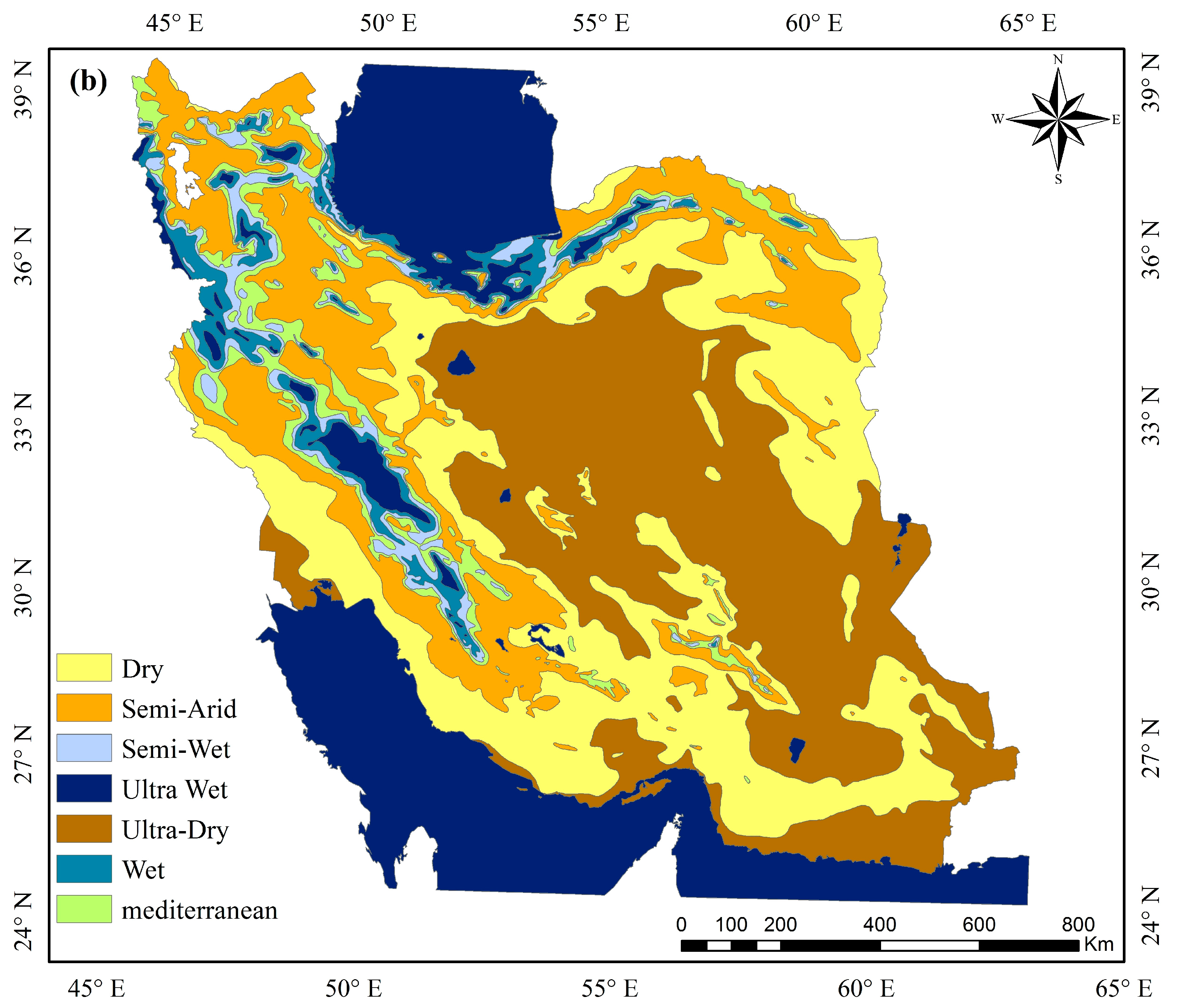
Iran is located in southwest Asia between 25°–40° north latitude and 44°–63° east longitude. Its population is 81 million and its area is approximately 1,648,195 km2. Located at an altitude of 40 to 5670 m above sea level, the altitude changes have a significant impact on the climatic diversity. Thus, Iran has a wide range of climatic conditions in different regions with significant rainfall variation. Annual rainfall decreases from northwest (900 mm) to southeast (200 mm). Rainstorms occur with great intensity during spring and have a high erosion potential [26]. Figure 1 shows the spatial distribution of synoptic stations and climate classification of Iran. Table 1 illustrates the geographical location of stations used to calculate the R-factor.
2.2. Climate Models
In recent years, simulations of the fifth phase of the Coupled Model Intercomparison Project (CMIP) have been completed [27]. and have been presented in the Fifth Assessment Report (AR5) by the Intergovernmental Panel on Climate Change (IPCC) [28]. The CMIP5 series models have higher resolution [29]. The greatest emphasis of these models is the climate impact on socio-economic issues and their role in sustainable development [30]. The general framework of these models is based on greenhouse gas reduction and climate adaptation methods [31].
These models use a new emission scenario to represent the greenhouse gas concentration path [32]. RCP scenarios include a severe reduction scenario (RCP2.6), and two intermediate scenarios (RCP4.5 and RCP6) and scenario (RCP8.5) [33]. These scenarios are named, based on their radiation level in 2100, which is 2.6, 4.5, 6, and 8.5 W/m2, respectively [34]. Table 2 illustrates the features of the four emission scenarios.
Due to the better performance of CMIP5 series models, many studies around the world have used these models [35,36]. In this study, precipitation data of CMIP5 models under RCP2.6 and RCP 8.5 scenarios were used to forcast future precipitation and its effect on rainfall erosion. Global Circulation Models (GCMs) are the most reliable models for forecasting climate and for simulating climate parameters [37]. These models are used for predicting climate change [38] and provide information about the Earth’s condition, including the state of atmosphere, carbon cycle, and circulation of oceans They can simulate climate change under RCP scenarios [39]. Although the models can predict future global climate change, their output has a high spatial resolution [40]. Therefore, application of these models on a local scale is not appropriate [41]. The high spatial resolution makes the model output unsuitable for investigating the hydrological effects of climate change on a regional scale [42].
Sixty-one climate models have been used to simulate the baseline and future periods in the fifth report of the Intergovernmental Panel on Climate Change (IPPC). In this study 4 models were used that included CSIRO-Mk3.6.0, CCSM4, GFDL-ESM2g, and HadGEM2-es SRES CPs [43] (Table 3). Using climatic parameters simulated by IPCC-CMIP5 series of models, possible changes in R-factor were estimated.
2.3. Downscaling Methods
Several methods have been proposed for downscaling the output of GCMs models [44]. In this research, the Delta or Change Factor (CF) downscaling method was used [45]. The change factor method is a common error correction method that is often used to reduce the error between GCM outputs and observational data [45] and is one of the simplest ways of statistical downscaling [46]. It is a ratio of changes between future forecasts and current climate simulations of a GCM model [47]. It uses monthly precipitation data recorded at synoptic stations. To obtain climate data on a local scale, the difference between precipitation ratios is used, based on the average of long-term monthly data for the future and current periods (base time). The CF values are calculated by dividing the average of each future weather month (evaluated by climate models) by the average of the same month at the base (recorded value of the synoptic station).
Precipitation parameter changes were calculated using the following equation [48]:
where indicates the scenario of climate change of precipitation parameter for 30 years, and is the number of months of a year that are between 1 and 12, defines the 20-year average precipitation simulated by GCMs for the future periods per month; describes the 30-year average precipitation simulated by the GCMs for the period similar to the base period for each month in this study is from 1986 to 2016.
To obtain the time series of future climate scenarios, the climate change scenarios were added to the observational values (1986–2016) that were obtained by the following equation [49]:
where Pobs describes the observed daily precipitation series in the 1986–2016 time period, P shows the time series of the future climate scenarios of precipitation, and defines the downscaled climate change scenarios.
In this study, the entire climate database was divided into four periods: the base time database was (1986–2016), the middle-time was (2046–2065), and the longtime future climate prediction was (2065–2081). Additionally, to evaluate precipitation forecasted by GCM, these forecasts were compared with the actual precipitation data recorded (1986–2016) at the synoptic stations.
2.4. Estimation of Rainfall-Runoff Erosivity (R-Factor)
To estimate rain erosivity (R-factor), the Revised Universal Soil Loss Equation (RUSLE) was used [50]. The RUSLE, revised as an experimental erosion model, is known as a standard method to estimate the mean risk of erosion on arable lands [51]. The Revised Universal Soil Loss Equation (RUSLE) has been developed by the U.S. Department of Agriculture Soil Conservation Service [52].
The RUSLE model estimates soil erosion as a combination of six factors that include rain erosivity (R), soil erodibility (K), slope length, and degree (LS), cultivation system (C), and management operations (P). This model was used to predict annual soil loss [52]
where E is the annual soil loss.
The most important factor to be investigated is the rainfall erosivity (R-factor), which was obtained using the following equation [53]:
in which denotes the average annual rainfall erosivity (), is the year’s number of data observations, defines the number of erosive events in the year, and defines the rainfall erosivity index of a storm K.
Studies have shown that the product of kinetic energy of rainstorm (E) and its maximum rainfall intensity of 30 min () is a suitable indicator for rainfall erosivity (R-factor). The index indicates the ability of rain to separate soil particles. The rainfall erosivity index () was calculated, based on the following Equation (3) [54]:
where defines rainstorm kinetic energy per unit height of the rainstorm (), and defines the height of rainstorm (mm).
where is the unit precipitation energy (), defines the rainstorm continuity (hr) in time , and describes the most precipitation intensity of 30 min ().
where is the rainfall intensity throughout the period ().
was calculated using the following equations:
where is the peak rain time, defines the rainfall duration, describes the base time of rainfall, is the maximum rainfall intensity, and is the rainfall.
R-factor was estimated using monthly and annual precipitation data recorded by Iranian synoptic stations for 32 years. The R-Factor values in Iran were between (1.17 and 5.5) compared to the R-factor values of the United States, which was in the range (20–550); it is very low, perhaps due to low rainfall [55].
2.5. Yearly Erosivity Density Ratio
According to Kinnell and [53], the erosion density coefficient is the R-factor ratio to precipitation. In practice, erosion is measured in units of precipitation (mm), the unit of which is MJ ha-1 h-1 that was obtained by the following equation:
where defines the erosion density, is the mean yearly precipitation erosivity, and describes the yearly rainfall.
2.6. Examination of R-Factor Performance
To validate the estimated R-factor, results were compared to the observational data of the synoptic stations by the following equations [56,57]:
The lower error between estimated and observed results shows that the RUSLE model has a good performance in estimating rainfall erosivity.
3. Results
3.1. Analysis of Future Precipitation
The output of climate models to predict rainfall erosivity is often biased toward the required scale [56]. Therefore, to evaluate the performance of these models in predicting climatic parameters, the statistical criteria presented in Section 2.6 were used. Table 4 illustrates the average absolute errors at all stations studied. Low RMSE and MAE values indicate better performance of models. Based on previous studies the RMSE values less than half of the SD (Standard Deviation) of the observed data (RMSE/Sdobs < 0.65) may be considered low and acceptable [58,59]. Based on Table 4, this equation applies.
Therefore, the CSIRO-Mk3.6.0 can forecast climate variables with low error.
Results showed that the CSIRO-Mk3.6.0 model had the best performance (minimum error), and then CCSM4, GFDL-ESM2g, and HadGEM2-es models had the best performance, respectively. According to the results of Table 4, the CSIRO-Mk3.6.0 model was selected as the best model for Ardabil, Bojnourd, Bushehr, Shahrekord, Isfahan, Qazvin, Gorgan, Ilam, Kermanshah, Sanandaj, Semnan, Shiraz, and Tabriz stations. At Arak, Urmia, Yasuj, and Mashhad stations, the CCSM4 model had the best results compared to the observational data. The data obtained from the GFDL-ESM2g model at Hamedan, Kerman, Khorramabad, Sari, Tehran, Yazd, Zanjan stations were most consistent with observational data. Other stations used the HadGEM2-es output.
3.2. Precipitation Prediction under Climate Change
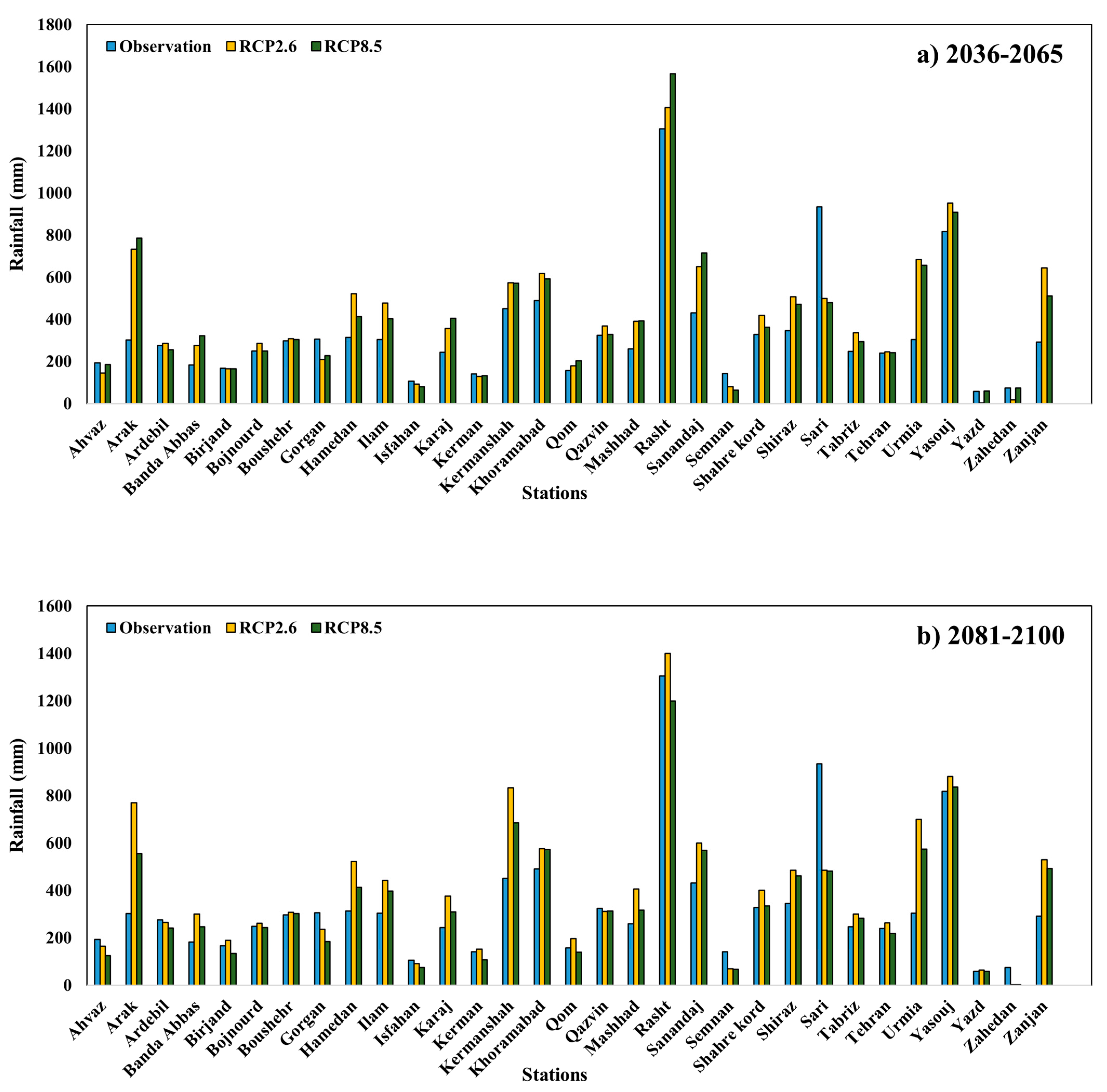
To assess the effect of different months of the year on rainfall erosivity, different months in the simulated periods and basis periods were compared. For this purpose, the average annual rainfall in the observed and simulated periods under RCP2.6 and RCP8.5 scenarios was used. Figure 2 shows the average annual precipitation predicted using the CSIRO-Mk3.6.0 model, during the near future (2046–2065) and the far future (2081–2100) under the RCP2.6 and RCP8.5 scenarios.
Results showed the selected models predicted an upward trend at some stations and a downward trend for precipitation at other stations. For example, the models predicted a decreasing trend for Semnan station compared with base times. Additionally, the models predicted an increasing trend of annual rainfall for Sanandaj station. Results of the models were moderately different from each other. Although the amount of rainfall at different stations during the near future (2046–2065) and the far future (2081–2100) under the RCP2.6 and RCP8.5 scenarios had different trends, the intensity of rainfall had a constantly increasing trend so that rainfall moved toward extreme precipitation which can increase the R-factor and can increase erosion in the coming years.
3.3. Spatial Distribution of R-Factor Erosivity in Current and Future Periods
Various studies have obtained R-factor using regression equations between precipitation and rainfall erosivity. To investigate the effect of climate change on rainfall erosivity, annual precipitation data was used. According to annual rainfall of each station and the values of relevant erosivity of rainfall, an appropriate regression relationship was selected. Table 5 illustrates the R-factor calculated by the equation for each station. In the equations, P defines the average annual precipitation, and R denotes the rainfall erosivity (MJ mm ha−1 h−1 year−1). Additionally, R2, MAE and RMSE were used to select the best regression relationship for the estimation of the R-factor of the Smith—Wischmeier method. Based on previous studies that RMSE values less than half of the SD (Standard Deviation) of the observed data (RMSE/SDobs < 0.65) may be considered low and acceptable [58,59]. Based on Table 4, this equation applies.
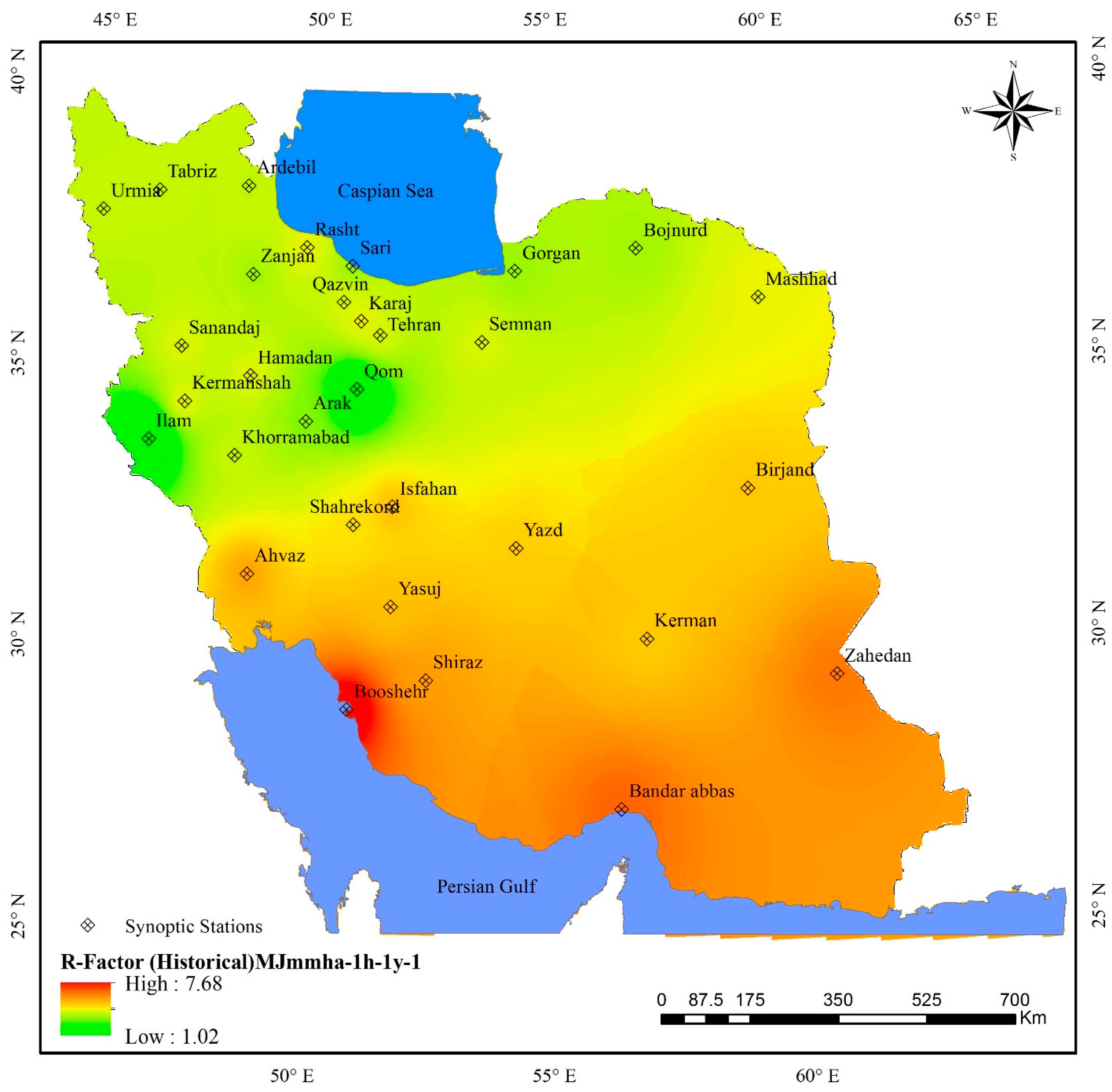
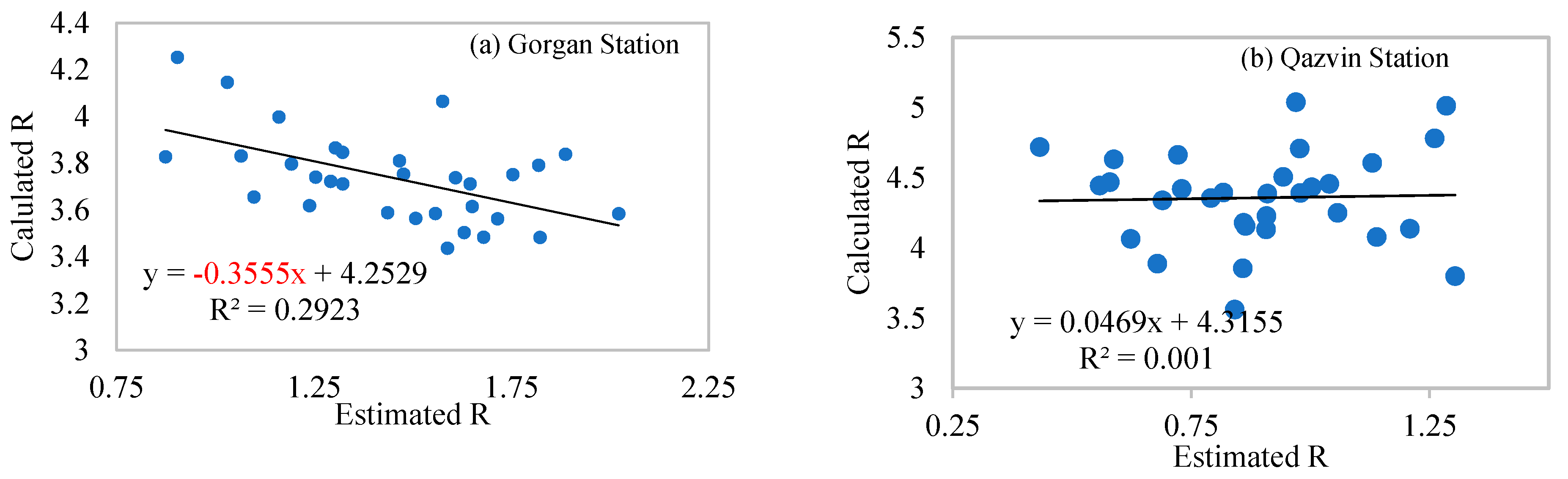
It is difficult to collect the data required to calculate the R-factor using the proposed method in all the regions of the country. The study of spatial variables of R-factor by these methods helps estimate the R-factor. Figure 3 shows the spatial distribution of R-factor for the historical period for all stations. Additionally, Figure 4 shows the scatter plot between observed and baseline annual rainfall erosivity values at sample Gorgan and Qazvin.
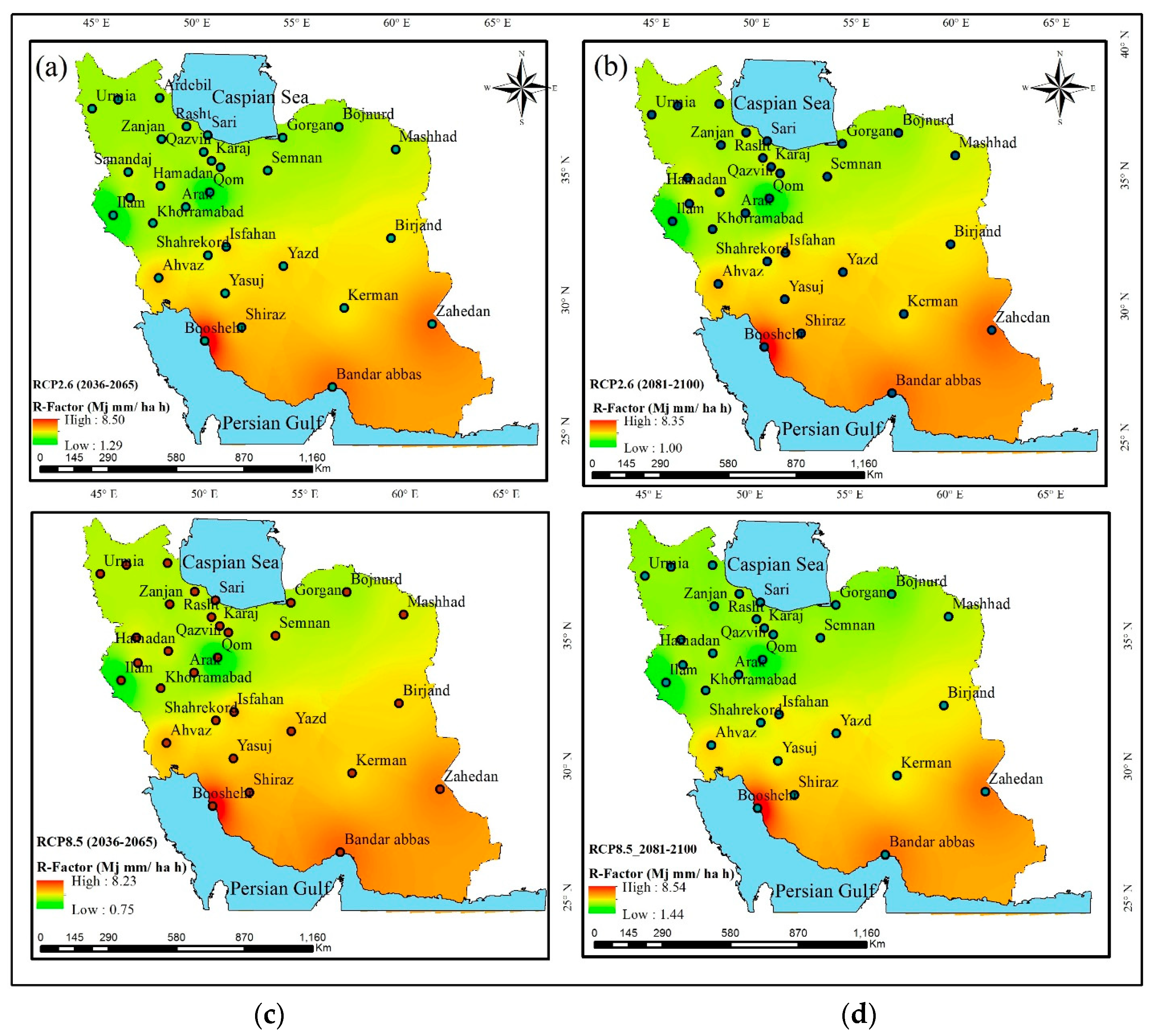
3.4. The Prediction of R-Factor under Climate Change
Using projected rainfall data, relative changes of mean annual R-factor were computed for future time periods (near and far-future) with respect to the baseline time period under two warming scenarios (RCP4.5 and RCP8.5). The spatial distributions of mean annual R-factor during the historical and the future time periods based on different scenarios are shown in Figure 5. Compared to the historical period, R-factor was expected to increase and decrease. It would change from 46.51% to 159% for the near future (2050), and from −48% to 154% for the far future (2090). In general, the central and southern regions of Iran are expected to have more climate change.
4. Discussion and Conclusions
The present study provides insights into the analysis of the R-factor for the historical and future periods under climate change in Iran.
In this study, four models CSIRO-Mk3.6.0, CCSM4, GFDL-ESM2g, HadGEM2-es from the 5th CMIP report were used for precipitation downscaling. Based on the obtained results, the CSIRO-Mk3.6.0 model had the lowest estimation error. The results of other researchers in the application of climate change models in Iran [45,60,61] confirmed this model.
Based on results, the average rainfall will increase significantly in the near and far future in the west of Iran. This situation is also significant for the southern regions of the country. However, a significant decrease is expected for the north of Iran, the southeast and some central regions. The results of other researchers [24,55,62,63] in Iran also confirmed these results.
Accordingly, the maximum difference in rainfall in the future was related to Arak station (483.82 mm), while the highest decrease was related to Sari station (453.51 mm). [14], also described the continued increase in rainfall during the 2050s and 2090s. Results showed significant variations in rainfall forecasts in western Iran.
Based on results, changes in precipitation compared to the historical period in the range of −51 mm and 48 mm were observed. Additionally, the most change under editer was under the RCP 8.5 scenario. Differences in the results indicated uncertainty in the scenarios as well as in the climate models used [64].
This study shows that the change in rainfall patterns has increased the R-factor the study area in recent times. Climate change has a significant impact on the R-factor. Precipitation rates are expected to increase in coming years, which could lead to increased R-factor and soil erosion rates. Additionally, it has been proven by [35,65,66] that the amount and intensity of the precipitation would have a negative effect on soil, so that it can increase the erosion rate.
Additionally, climate change can significantly affect land cover, which can reinforce a particular process of erosion. To predict future rainfall erosivity and soil erosion trends, the interaction between rainfall and land cover must be evaluated.
Considering the effect of climate change, soil erosion will increase in all parts of Iran in the future compared to the base period. According to the obtained results, the vulnerability of central and southern parts of Iran is more than of the northern parts, so twice as much management is required.
Author Contributions
Conceptualization, B.F. and O.B.; methodology, O.B. and V.P.S.; software, S.C. and B.F.; validation, O.B. and V.P.S.; formal analysis, O.B and S.C.; investigation, B.F. and M.M.S.; resources, B.F.; data curation, V.P.S. and M.M.S.; writing original draft preparation, S.C. and O.B.; writing—review and editing, B.F. and O.B.; visualization, O.B.; funding acquisition, M.M.S. All authors have read and agreed to the published version of the manuscript.
Funding
This research was funded by Iranian National Science Foundation (INSF) grant number: 95849555.
Data Availability Statement
The datasets generated during and/or analyzed during the current study are available from the corresponding author on reasonable request.
Conflicts of Interest
The authors declare no conflict of interest.
References
- Talchabhadel, R.; Nakagawa, H.; Kawaike, K.; Prajapati, R. Evaluating the rainfall erosivity (R-factor) from daily rainfall data: An application for assessing climate change impact on soil loss in Westrapti River basin, Nepal. Model. Earth Syst. Environ. 2020, 6, 1741–1762. [Google Scholar] [CrossRef]
- Jackson, R.B.; Saunois, M.; Bousquet, P.; Canadell, J.G.; Poulter, B.; Stavert, A.R.; Bergamaschi, P.; Niwa, Y.; Segers, A.; Tsuruta, A. Increasing anthropogenic methane emissions arise equally from agricultural and fossil fuel sources. Environ. Res. Lett. 2020, 15, 071002. [Google Scholar] [CrossRef]
- Shin, J.-Y.; Kim, K.R.; Ha, J.-C. Seasonal forecasting of daily mean air temperatures using a coupled global climate model and machine learning algorithm for field-scale agricultural management. Agric. For. Meteorol. 2020, 281, 107858. [Google Scholar] [CrossRef]
- Pandey, D. Agricultural Sustainability and Climate Change Nexus. In Contemporary Environmental Issues and Challenges in Era of Climate Change; Springer: Singapore, 2020; pp. 77–97. [Google Scholar]
- Chen, X.; Zhu, H.; Yan, B.; Shutes, B.; Xing, D.; Banuelos, G.; Cheng, R.; Wang, X. Greenhouse gas emissions and wastewater treatment performance by three plant species in subsurface flow constructed wetland mesocosms. Chemosphere 2020, 239, 124795. [Google Scholar] [CrossRef] [PubMed]
- Zhang, Y.; Ayyub, B.M. Electricity System Assessment and Adaptation to Rising Temperatures in a Changing Climate Using Washington Metro Area as a Case Study. J. Infrastruct. Syst. 2020, 26, 04020017. [Google Scholar] [CrossRef]
- Siegert, M.; Alley, R.B.; Rignot, E.; Englander, J.; Corell, R. Twenty-first century sea-level rise could exceed IPCC projections for strong-warming futures. One Earth 2020, 3, 691–703. [Google Scholar] [CrossRef]
- Konapala, G.; Mishra, A.K.; Wada, Y.; Mann, M.E. Climate change will affect global water availability through compounding changes in seasonal precipitation and evaporation. Nat. Commun. 2020, 11, 3044. [Google Scholar] [CrossRef]
- Schädler, M.; Buscot, F.; Klotz, S.; Reitz, T.; Durka, W.; Bumberger, J.; Merbach, I.; Michalski, S.G.; Kirsch, K.; Remmler, P.; et al. Investigating the consequences of climate change under different land-use regimes: A novel experimental infrastructure. Ecosphere 2019, 10, e02635. [Google Scholar] [CrossRef] [Green Version]
- Barton, M.G.; Terblanche, J.S.; Sinclair, B.J. Incorporating temperature and precipitation extremes into process-based models of African lepidoptera changes the predicted distribution under climate change. Ecol. Model. 2019, 394, 53–65. [Google Scholar] [CrossRef]
- Nearing, M.A.; Pruski, F.F.; O’Neal, M.R. Expected climate change impacts on soil erosion rates: A review. J. Soil Water Conserv. 2004, 59, 43–50. [Google Scholar]
- Simonneaux, V.; Cheggour, A.; Deschamps, C.; Mouillot, F.; Cerdan, O.; Le Bissonnais, Y. Land use and climate change effects on soil erosion in a semi-aridmountainous watershed (High Atlas, Morocco). J. Arid Environ. 2015, 122, 64–75. [Google Scholar] [CrossRef]
- Morán-Ordóñez, A.; Duane, A.; Gil-Tena, A.; De Cáceres, M.; Aquilué, N.; Guerra, C.A.; Geijzendorffer, I.R.; Fortin, M.; Brotons, L. Future impact of climate extremes in the Mediterranean: Soil erosion projections when fire and extreme rainfall meet. Land Degrad. Dev. 2020, 31, 3040–3054. [Google Scholar] [CrossRef]
- Gafforov, K.S.; Bao, A.; Rakhimov, S.; Liu, T.; Abdullaev, F.; Jiang, L.; Durdiev, K.; Duulatov, E.; Rakhimova, M.; Mukanov, Y. The assessment of climate change on rainfall-runoff erosivity in the Chirchik–Akhangaran Basin, Uzbekistan. Sustainability 2020, 12, 3369. [Google Scholar] [CrossRef] [Green Version]
- Kastridis, A.; Stathis, D.; Sapountzis, M.; Theodosiou, G. Insect outbreak and long-term post-fire effects on soil erosion editerraneanean suburban forest. Land 2022, 11, 911. [Google Scholar] [CrossRef]
- de Almeida, W.S.; Seitz, S.; de Oliveira, L.F.C.; de Carvalho, D.F. Duration and intensity of rainfall events with the same erosivity change sediment yield and runoff rates. Int. Soil Water Conserv. Res. 2021, 9, 69–75. [Google Scholar] [CrossRef]
- Kinnell, P.; Yu, B. CLIGEN as a weather generator for predicting rainfall erosion using USLE based modelling systems. Catena 2020, 194, 104745. [Google Scholar] [CrossRef]
- Grillakis, M.G.; Polykretis, C.; Alexakis, D.D. Past and projected climate change impacts on rainfall erosivity: Advancing our knowledge for the eastern Mediterranean island of Crete. Catena 2020, 193, 104625. [Google Scholar] [CrossRef]
- Liu, Y.; Zhao, W.; Liu, Y.; Pereira, P. Global rainfall erosivity changes between 1980 and 2017 based on an erosivity model using daily precipitation data. Catena 2020, 194, 104768. [Google Scholar] [CrossRef]
- Riquetti, N.B.; Mello, C.R.; Beskow, S.; Viola, M.R. Rainfall erosivity in South America: Current patterns and future perspectives. Sci. Total. Environ. 2020, 724, 138315. [Google Scholar] [CrossRef]
- Nasidi, N.M.; Wayayok, A.; Abdullah, A.F.; Kassim, M.S.M. Spatio-temporal dynamics of rainfall erosivity due to climate change in Cameron Highlands, Malaysia. Model. Earth Syst. Environ. 2021, 7, 1847–1861. [Google Scholar] [CrossRef]
- Almagro, A.; Oliveira, P.T.; Nearing, M.A.; Hagemann, S. Projected climate change impacts in rainfall erosivity over Brazil. Sci. Rep. 2017, 7, 8130. [Google Scholar] [CrossRef]
- Xu, Y.; Sun, H.; Ji, X. Spatial-temporal evolution and driving forces of rainfall erosivity in a climatic transitional zone: A case in Huaihe River Basin, eastern China. Catena 2021, 198, 104993. [Google Scholar] [CrossRef]
- Azhdari, Z.; Sardooi, E.R.; Bazrafshan, O.; Zamani, H.; Singh, V.P.; Saravi, M.M.; Ramezani, M. Impact of climate change on net primary production (NPP) in south Iran. Environ. Monit. Assess. 2020, 192, 409. [Google Scholar] [CrossRef] [PubMed]
- Chakrabortty, R.; Pradhan, B.; Mondal, P.; Pal, S.C. The use of RUSLE and GCMs to predict potential soil erosion associated with climate change in a monsoon-dominated region of eastern India. Arab. J. Geosci. 2020, 13, 1073. [Google Scholar] [CrossRef]
- Sadeghi, S.H.R.; Hazbavi, Z. Trend analysis of the rainfall erosivity index at different time scales in Iran. Nat. Hazards 2015, 77, 383–404. [Google Scholar] [CrossRef]
- Fiedler, S.; Crueger, T.; D’Agostino, R.; Peters, K.; Becker, T.; Leutwyler, D.; Paccini, L.; Burdanowitz, J.; Buehler, S.A.; Cortes, A.U.; et al. Simulated Tropical Precipitation Assessed across Three Major Phases of the Coupled Model Intercomparison Project (CMIP). Mon. Weather Rev. 2020, 148, 3653–3680. [Google Scholar] [CrossRef]
- Emori, S.; Taylor, K.; Hewitson, B.; Zermoglio, F.; Juckes, M.; Lautenschlager, M.; Stockhause, M. CMIP5 Data Provided at the IPCC Data Distribution Centre. In Fact Sheet of the Task Group on Data and Scenario Support for Impact and Climate Analysis (TGICA) of The Intergovernmental Panel on Climate Change (IPCC); IPCC: Geneva, Switzerland, 2016. [Google Scholar]
- Aghakhaniafshar, A.; Hasanzadeh, Y.; Pourreza-Bilondi, A.A.B.M. Seasonal changes of precipitation and temperature of mountainous watersheds in future periods with approach of fifth report of Intergovernmental Panel on Climate Change (case study: Kashafrood Watershed Basin). J. Water Soil 2016, 30, 1718–1732. [Google Scholar]
- Burke, E.J.; Zhang, Y.; Krinner, G. Evaluating permafrost physics in the Coupled Model Intercomparison Project 6 (CMIP6) models and their sensitivity to climate change. Cryosphere 2020, 14, 3155–3174. [Google Scholar] [CrossRef]
- Colorado-Ruiz, G.; Cavazos, T.; Salinas, J.A.; De Grau, P.; Ayala, R. Climate change projections from Coupled Model Intercomparison Project phase 5 multi-model weighted ensembles for Mexico, the North American monsoon, and the mid-summer drought region. Int. J. Clim. 2018, 38, 5699–5716. [Google Scholar] [CrossRef]
- Wandres, M.; Pattiaratchi, C.; Hemer, M.A. Projected changes of the southwest Australian wave climate under two atmospheric greenhouse gas concentration pathways. Ocean Model. 2017, 117, 70–87. [Google Scholar] [CrossRef]
- Sánchez-García, D.; Bienvenido-Huertas, D.; Pulido-Arcas, J.A.; Rubio-Bellido, C. Analysis of Energy Consumption in Different European Cities: The Adaptive Comfort Control Implemented Model (ACCIM) Considering Representative Concentration Pathways (RCP) Scenarios. Appl. Sci. 2020, 10, 1513. [Google Scholar] [CrossRef] [Green Version]
- Zhang, Y.; You, Q.; Chen, C.; Ge, J. Impacts of climate change on streamflows under RCP scenarios: A case study in Xin River Basin, China. Atmospheric Res. 2016, 178–179, 521–534. [Google Scholar] [CrossRef]
- Gupta, A.S.; Jourdain, N.; Brown, J.N.; Monselesan, D. Climate Drift in the CMIP5 Models. J. Clim. 2013, 26, 8597–8615. [Google Scholar] [CrossRef] [Green Version]
- Tranu, L. Projections of changes in productivity of major agricultural crops in the Republic of Moldova according to CMIP5 ensemble of 21 GCMs for RCP2. 6, RCP4. 5 and RCP8. 5 scenarios. Sci. Pap. Ser. A Agron. 2016, 59, 431–440. [Google Scholar]
- Balov, M.N.; Altunkaynak, A. Spatio-temporal evaluation of various global circulation models in terms of projection of different meteorological drought indices. Environ. Earth Sci. 2020, 79, 126. [Google Scholar] [CrossRef]
- Akinsanola, A.; Ajayi, V.; Adejare, A.; Adeyeri, O.; Gbode, I.; Ogunjobi, K.; Nikulin, G.; Abolude, A. Evaluation of rainfall simulations over West Africa in dynamically downscaled CMIP5 global circulation models. Theor. Appl. Climatol. 2017, 132, 437–450. [Google Scholar] [CrossRef]
- Shrestha, S.; Bach, T.V.; Pandey, V.P. Climate change impacts on groundwater resources in Mekong Delta under repre-sentative concentration pathways (RCPs) scenarios. Environ. Sci. Policy 2016, 61, 1–13. [Google Scholar] [CrossRef]
- Adeniyi, M.O. The consequences of the IPCC AR5 RCPs 4.5 and 8.5 climate change scenarios on precipitation in West Africa. Clim. Chang. 2016, 139, 245–263. [Google Scholar] [CrossRef]
- Murakami, H.; Vecchi, G.; Villarini, G.; Delworth, T.; Gudgel, R.; Underwood, S.; Yang, X.; Zhang, W.; Lin, S.-J. Seasonal Forecasts of Major Hurricanes and Landfalling Tropical Cyclones using a High-Resolution GFDL Coupled Climate Model. J. Clim. 2016, 29, 7977–7989. [Google Scholar] [CrossRef]
- Gallina, V.; Torresan, S.; Zabeo, A.; Rizzi, J.; Carniel, S.; Sclavo, M.; Pizzol, L.; Marcomini, A.; Critto, A. Assessment of Climate Change Impacts in the North Adriatic Coastal Area. Part II: Consequences for Coastal Erosion Impacts at the Regional Scale. Water 2019, 11, 1300. [Google Scholar] [CrossRef] [Green Version]
- Zhu, Q.; Yang, X.; Ji, F.; Liu, D.L.; Yu, Q. Extreme rainfall, rainfall erosivity, and hillslope erosion in Australian Alpine region and their future changes. Int. J. Clim. 2019, 40, 1213–1227. [Google Scholar] [CrossRef]
- Nourani, V.; Paknezhad, N.J.; Sharghi, E.; Khosravi, A. Estimation of prediction interval in ANN-based multi-GCMs downscaling of hydro-climatologic parameters. J. Hydrol. 2019, 579, 124226. [Google Scholar] [CrossRef]
- Kimiagar, V.; Fattahi, E.; Alimohammadi, S. Analyzing effect of different statistical downscaling methods on the predicted streamflow in Karaj dam basin under climate change effect. J. Clim. Res. 2020, 1398, 17–31. [Google Scholar]
- Meresa, H.; Murphy, C.; Fealy, R.; Golian, S. Uncertainties and their interaction in flood risk assessment with climate change. Hydrol. Earth Syst. Sci. Discuss. 2020, 2020, 1–35. [Google Scholar] [CrossRef]
- Wootten, A.M.; Dixon, K.W.; Adams-Smith, D.J.; McPherson, R.A. Statistically downscaled precipitation sensitivity to gridded observation data and downscaling technique. Int. J. Clim. 2021, 41, 980–1001. [Google Scholar] [CrossRef]
- Van Uytven, E.; Wampers, E.; Wolfs, V.; Willems, P. Evaluation of change factor-based statistical downscaling methods for impact analysis in urban hydrology. Urban Water J. 2020, 17, 785–794. [Google Scholar] [CrossRef]
- Dixon, K.; Adams-Smith, D.; Lanzante, J. On the Sensitivity of 21st Century Spring Plant Phenology Projections to the Choice Of Statistical Downscaling Method. In Proceedings of the EGU General Assembly Conference, Virtual, 4–8 May 2020; Abstracts. p. 3776. [Google Scholar]
- Maqsoom, A.; Aslam, B.; Hassan, U.; Kazmi, Z.A.; Sodangi, M.; Tufail, R.F.; Farooq, D. Geospatial Assessment of Soil Erosion Intensity and Sediment Yield Using the Revised Universal Soil Loss Equation (RUSLE) Model. ISPRS Int. J. Geo-Inf. 2020, 9, 356. [Google Scholar] [CrossRef]
- Albut, S. Determination of R Factor in Revised Universal Soil Loss Equation (RUSLE) With Open Sources Geographical Information System (GIS) Software. J. Multidiscip. Eng. Sci. Technol. 2020, 7, 12507–12510. [Google Scholar]
- Nehaï, S.A.; Guettouche, M.S. Soil loss estimation using the revised universal soil loss equation and a GIS-based model: A case study of Jijel Wilaya, Algeria. Arab. J. Geosci. 2020, 13, 152. [Google Scholar] [CrossRef]
- Yue, T.; Xie, Y.; Yin, S.; Yu, B.; Miao, C.; Wang, W. Effect of time resolution of rainfall measurements on the erosivity factor in the USLE in China. Int. Soil Water Conserv. Res. 2020, 8, 373–382. [Google Scholar] [CrossRef]
- Girmay, G.; Moges, A.; Muluneh, A. Estimation of soil loss rate using the USLE model for Agewmariayam Watershed, northern Ethiopia. Agric. Food Secur. 2020, 9, 9. [Google Scholar] [CrossRef]
- Azari, M.; Oliaye, A.; Nearing, M.A. Expected climate change impacts on rainfall erosivity over Iran based on CMIP5 climate models. J. Hydrol. 2021, 593, 125826. [Google Scholar] [CrossRef]
- Panagos, P.; Borrelli, P.; Meusburger, K.; Yu, B.; Klik, A.; Lim, K.J.; Yang, J.E.; Ni, J.; Miao, C.; Chattopadhyay, N.; et al. Global rainfall erosivity assessment based on high-temporal resolution rainfall records. Sci. Rep. 2017, 7, 4175. [Google Scholar] [CrossRef] [PubMed] [Green Version]
- Duulatov, E.; Chen, X.; Amanambu, A.C.; Ochege, F.U.; Orozbaev, R.; Issanova, G.; Omurakunova, G. Projected Rainfall Erosivity Over Central Asia Based on CMIP5 Climate Models. Water 2019, 11, 897. [Google Scholar] [CrossRef] [Green Version]
- Margiorou, S.; Kastridis, A.; Sapountzis, M. Pre/Post-Fire Soil Erosion and Evaluation of Check-Dams Effectiveness in Mediterranean Suburban Catchments Based on Field Measurements and Modeling. Land 2022, 11, 1705. [Google Scholar] [CrossRef]
- Singh, J.; Knapp, H.V.; Arnold, J.G.; Demissie, M. Hydrological modeling of the Iroquois river watershed using HSPF and SWAT. J. Am. Water Resour. Assoc. 2005, 41, 343–360. [Google Scholar] [CrossRef]
- Samadi, S.; Sagareswar, G.; Tajiki, M. Comparison of General Circulation Models: Methodology for selecting the best GCM in Kermanshah Synoptic Station, Iran. Int. J. Glob. Warm. 2010, 2, 347–365. [Google Scholar] [CrossRef]
- Keteklahijani, V.K.; Alimohammadi, S.; Fattahi, E. Predicting changes in monthly streamflow to Karaj dam res-ervoir, Iran, in climate change condition and assessing its uncertainty. Ain Shams Eng. J. 2019, 10, 669–679. [Google Scholar] [CrossRef]
- Zarghami, M.; Abdi, A.; Babaeian, I.; Hassanzadeh, Y.; Kanani, R. Impacts of climate change on runoffs in East Azerbaijan, Iran. Glob. Planet. Chang. 2011, 78, 137–146. [Google Scholar] [CrossRef]
- Azimi Sardari, M.R.A.; Bazrafshan, O.; Panagopoulos, T.; Sardooi, E.R. Modeling the Impact of Climate Change and Land Use Change Scenarios on Soil Erosion at the Minab Dam Watershed. Sustainability 2019, 11, 3353. [Google Scholar] [CrossRef] [Green Version]
- Sharafati, A.; Pezeshki, E. A strategy to assess the uncertainty of a climate change impact on extreme hydrological events in the semi-arid Dehbar catchment in Iran. Theor. Appl. Climatol. 2019, 139, 389–402. [Google Scholar] [CrossRef]
- Litschert, S.; Theobald, D.; Brown, T. Effects of climate change and wildfire on soil loss in the Southern Rockies Ecoregion. Catena 2014, 118, 206–219. [Google Scholar] [CrossRef]
- Amanambu, A.C.; Li, L.; Egbinola, C.N.; Obarein, O.A.; Mupenzi, C.; Chen, D. Spatio-temporal variation in rain-fall-runoff erosivity due to climate change in the Lower Niger Basin, West Africa. Catena 2019, 172, 324–334. [Google Scholar] [CrossRef]
Figure 1.
Spatial distribution of synoptic station (a), Climate Classification (b).


Figure 2.
Mean relative change of mean annual precipitation projected by the selected model for the future period (2046–2065 (a) and 2081–2100 (b)) compared to the historical period (1986–2016).
Figure 2.
Mean relative change of mean annual precipitation projected by the selected model for the future period (2046–2065 (a) and 2081–2100 (b)) compared to the historical period (1986–2016).

Figure 3.
Rainfall erosivity in historical period.

Figure 4.
Scatter plot between observed and baseline annual rainfall erosivity at (a) Gorgan and (b) Qazvin station.
Figure 4.
Scatter plot between observed and baseline annual rainfall erosivity at (a) Gorgan and (b) Qazvin station.

Figure 5.
Rainfall erosivity projections for the period 2050s and 2090s under RCP2.6 and 8.5 scenarios, (a) (RCP2.6 (2036–2065)); (b) (RCP 2.6 (2081–2100)); (c) (RCP8.5 (2036–2065)) and (d) (RCP8.5 (2081–2100)).
Figure 5.
Rainfall erosivity projections for the period 2050s and 2090s under RCP2.6 and 8.5 scenarios, (a) (RCP2.6 (2036–2065)); (b) (RCP 2.6 (2081–2100)); (c) (RCP8.5 (2036–2065)) and (d) (RCP8.5 (2081–2100)).


Table 1.
Stations with high-resolution data to calculate the R-factor.
| Station | Elevation | Longitude | Latitude |
|---|---|---|---|
| Ahvaz | 22.5 | 48°40′ | 31°20′ |
| Arak | 1708 | 49°46′ | 34°06′ |
| Ardebil | 1332 | 48°17′ | 38°15′ |
| Banda Abbas | 9.8 | 56°22′ | 27°13′ |
| Birjand | 1491 | 59°12′ | 32°52′ |
| Bojnourd | 1112 | 57°16′ | 37°28′ |
| Boushehr | 19.6 | 50°50′ | 28°59′ |
| Gorgan | 13.3 | 54°16′ | 36°51′ |
| Hamedan | 1679 | 48°43′ | 35°12′ |
| Ilam | 1337 | 46°26′ | 33°38′ |
| Isfahan | 1550 | 51°40′ | 32°37′ |
| Karaj | 1312 | 50°54′ | 35°55′ |
| Kerman | 1753 | 56°58′ | 30°15′ |
| Kermanshah | 1318 | 47°09′ | 34°24′ |
| Khoramabad | 1147 | 48°17′ | 33°26′ |
| Qom | 877 | 50°51′ | 32°42′ |
| Qazvin | 1279 | 50°03′ | 36°15′ |
| Mashhad | 999 | 59°38′ | 36°16′ |
| Rasht | 36.7 | 49°39′ | 37°12′ |
| Sanandaj | 1373 | 47°00′ | 35°20′ |
| Semnan | 1130 | 53°33′ | 35°35′ |
| Shahre kord | 2048 | 50°51′ | 32°17′ |
| Shiraz | 1484 | 52°36′ | 29°32′ |
| Sari | 23 | 53°00′ | 36°33′ |
| Tabriz | 1361 | 46°17′ | 38°50′ |
| Tehran | 1190 | 51°19′ | 35°41′ |
| Urmia | 1315 | 45°05′ | 37°32′ |
| Yasouj | 1831 | 51°41′ | 30°50′ |
| Yazd | 1273 | 54°17′ | 31°54′ |
| Zahedan | 1370 | 60°33′ | 29°28′ |
| Zanjan | 1663 | 48°29′ | 36°41′ |
Table 2.
Features of Representative Concentration Pathway (RCPs).
| Scenarios | Radiative Forcing | Concentration of Carbon Dioxide(ppm) | Temperature (C°) | Pathway |
|---|---|---|---|---|
| RCP2.6 | 3 W/m2 | 490–530 | 1.5 | Peak and Decline |
| RCP4.5 | 4.5 W/m2 | 580–720 | 2.4 | Stabilization without overshoot pathway |
| RCP6 | 6 W/m2 | 720–1000 | 3 | Stabilization without overshoot pathway |
| RCP8.5 | 8.5 W/m2 | 4.8 | Rising radiative forcing pathway |
Table 3.
Specification of CMIP5 series models used in this study.
| Models | Institute | Resolution |
|---|---|---|
| CSIRO-Mk3.6.0 | Commonwealth Scientific and Industrial Research Organization (CSIRO), Canberra, Australia | 1.88° × 1.88° |
| CCSM4 | National Center for Atmospheric Research (NSAR), Boulder, CO, USA | 1.25° × 0.94° |
| GFDL-ESM2g | Geophysical Fluid Dynamics Laboratory (NOAA), Princeton, NJ, USA | 2.00° × 2.02° |
| HadGEM2-es | Met Office Hadley Center (MOHC), Exeter, UK | 1.88° × 1.25° |
Table 4.
Evaluation error index for precipitation of each station in historical duration.
| Station | Model | RMSE | RMSE/SD < 0.65 | MAE | Station | RMSE | RMSE/SD < 0.65 | MAE |
|---|---|---|---|---|---|---|---|---|
| Ardebil | GFDL-ESM2g | 10.64 | 0.43 | 8.32 | Hamedan | 15.57 | 0.29 | 12.33 |
| HadGEM2-es | 69.39 | 2.83 | 38.15 | 42.06 | 0.78 | 136.63 | ||
| CSIRO-Mk3.6.0 | 10.1 | 0.41 | 8.31 | 29.03 | 0.54 | 21.73 | ||
| CCSM4 | 10.33 | 0.42 | 8.31 | 20.76 | 0.38 | 14.17 | ||
| SD observed | 24.5 | - | - | - | 54 | - | - | |
| Arak | GFDL-ESM2g | 10.28 | 0.27 | 6.76 | Ilam | 38.5 | 0.44 | 62.58 |
| HadGEM2-es | 260.71 | 6.95 | 89.92 | 54.5 | 0.63 | 161.13 | ||
| CSIRO-Mk3.6.0 | 10.4 | 0.28 | 14.38 | 10.11 | 0.12 | 8.3 | ||
| CCSM4 | 11.44 | 0.31 | 8.54 | 136.74 | 1.57 | 49.44 | ||
| SD observed | 37.5 | - | - | - | 87 | - | - | |
| Urmia | GFDL-ESM2g | 15.64 | 0.12 | 11.82 | Karaj | 10.56 | 0.10 | 7.1 |
| HadGEM2-es | 270.27 | 2.05 | 88.4 | 19.09 | 0.19 | 12.79 | ||
| CSIRO-Mk3.6.0 | 11.2 | 0.08 | 11.95 | 8.6 | 0.09 | 12.66 | ||
| CCSM4 | 12.84 | 0.10 | 9.24 | 9.06 | 0.09 | 4.97 | ||
| SD observed | 132 | - | - | - | 101 | - | - | |
| Bandar abbas | GFDL-ESM2g | 18.76 | 0.18 | 11.94 | Kerman | 8 | 0.14 | 4.97 |
| HadGEM2-es | 108.99 | 1.04 | 45.63 | 11.5 | 0.20 | 7.57 | ||
| CSIRO-Mk3.6.0 | 20.1 | 0.19 | 14.14 | 7.2 | 0.12 | 6.98 | ||
| CCSM4 | 20.36 | 0.19 | 12.14 | 8.46 | 0.15 | 5.04 | ||
| SD observed | 105 | - | - | - | 58 | - | - | |
| Birjand | GFDL-ESM2g | 7.32 | 0.42 | 3.82 | Kermanshah | 41.24 | 0.21 | 17.54 |
| HadGEM2-es | 24.84 | 1.42 | 14.66 | 73.45 | 0.37 | 21.32 | ||
| CSIRO-Mk3.6.0 | 6.53 | 0.37 | 5.08 | 24 | 0.12 | 11.25 | ||
| CCSM4 | 7.04 | 0.40 | 4.02 | 25.11 | 0.13 | 17.58 | ||
| SD observed | 17.5 | - | - | - | 198 | - | - | |
| Bojnourd | GFDL-ESM2g | 11.52 | 0.18 | 7.78 | Khorram abad | 8.05 | 0.06 | 4.97 |
| HadGEM2-es | 22.27 | 0.34 | 15.18 | 11.5 | 0.09 | 7.57 | ||
| CSIRO-Mk3.6.0 | 10.9 | 0.17 | 8.89 | 11.2 | 0.08 | 6.98 | ||
| CCSM4 | 21.76 | 0.33 | 15.82 | 8.46 | 0.06 | 5.04 | ||
| SD observed | 65 | - | - | - | 135 | - | - | |
| Boushehr | GFDL-ESM2g | 83.75 | 0.88 | 142.12 | Ahvaz | 25.24 | 0.20 | 16.4 |
| HadGEM2-es | 70.3 | 0.74 | 287.07 | 85.45 | 0.68 | 36.35 | ||
| CSIRO-Mk3.6.0 | 19.17 | 0.20 | 16.2 | 29.04 | 0.23 | 21.25 | ||
| CCSM4 | 34.3 | 0.36 | 34.3 | 29.49 | 0.24 | 17.58 | ||
| SD observed | 95 | - | - | - | 125 | - | - | |
| Shahre kord | GFDL-ESM2g | 2.65 | 0.10 | 16.15 | Yasuj | 1.44 | 0.06 | 16.19 |
| HadGEM2-es | 6.36 | 0.24 | 52.17 | 6.36 | 0.25 | 75.17 | ||
| CSIRO-Mk3.6.0 | 9.6 | 0.36 | 7.65 | 5.4 | 0.22 | 15.65 | ||
| CCSM4 | 5.6 | 0.21 | 12.85 | 5.68 | 0.23 | 10.82 | ||
| SD observed | 27 | - | - | - | 25 | - | - | |
| Isfahan | GFDL-ESM2g | 5.67 | 0.16 | 4.13 | Mashahd | 58.55 | 2.34 | 34.05 |
| HadGEM2-es | 64.61 | 1.82 | 29.48 | 10.96 | 0.44 | 8.94 | ||
| CSIRO-Mk3.6.0 | 5.1 | 0.14 | 3.62 | 7.8 | 0.31 | 11.51 | ||
| CCSM4 | 5.86 | 0.17 | 4.73 | 8.88 | 0.36 | 7.51 | ||
| SD observed | 35.5 | - | - | - | 25 | - | - | |
| Qom | GFDL-ESM2g | 11.11 | 0.13 | 7.15 | Sanandaj | 41.45 | 0.92 | 17.15 |
| HadGEM2-es | 16.2 | 0.19 | 15.12 | 68.85 | 1.53 | 22.41 | ||
| CSIRO-Mk3.6.0 | 19.52 | 0.23 | 15.65 | 21.2 | 0.47 | 13.89 | ||
| CCSM4 | 8.56 | 0.10 | 7.85 | 22.11 | 0.49 | 16.75 | ||
| SD observed | 84 | - | - | - | 45 | - | - | |
| Qazvin | GFDL-ESM2g | 7.25 | 0.12 | 7.8 | Semnan | 6.58 | 0.14 | 5.15 |
| HadGEM2-es | 9.59 | 0.15 | 12.65 | 6.4 | 0.14 | 36.65 | ||
| CSIRO-Mk3.6.0 | 7.75 | 0.12 | 8.81 | 5.1 | 0.11 | 3.62 | ||
| CCSM4 | 6.71 | 0.11 | 8.91 | 5.21 | 0.11 | 4.51 | ||
| SD observed | 63 | - | - | - | 47 | - | - | |
| Gorgan | GFDL-ESM2g | 13.39 | 0.23 | 9.58 | Shiraz | 3.52 | 0.05 | 19.19 |
| HadGEM2-es | 29.95 | 0.52 | 19.35 | 9.98 | 0.15 | 25.17 | ||
| CSIRO-Mk3.6.0 | 24.59 | 0.42 | 16.5 | 1.2 | 0.02 | 7.85 | ||
| CCSM4 | 13.39 | 0.23 | 11.4 | 7.61 | 0.12 | 11.12 | ||
| SD observed | 58 | - | - | - | 65 | - | - |
Table 5.
Relationship between indices of yearly precipitation and erosivity factor and evaluation of radial basis function to estimate rainfall erosivity index.
Table 5.
Relationship between indices of yearly precipitation and erosivity factor and evaluation of radial basis function to estimate rainfall erosivity index.
| Station | Regression Equations | R2 | RMSE | SD | RMSE/SD < 0.65 | MAE |
|---|---|---|---|---|---|---|
| Ahvaz | R = 0.111P + 5.50 | 0.68 | 0.6 | 1.2 | 0.5 | 0.08 |
| Arak | R = −0.4406P + 4.9161 | 0.55 | 0.29 | 2.33 | 0.12446352 | 0.08 |
| Ardebil | R = −2.6982P2 + 4.423P + 2.29 | 0.87 | 0.26 | 2.65 | 0.09811321 | 0.04 |
| Banda Abbas | R = −0.5223P + 7.15 | 0.85 | 1.12 | 2.68 | 0.41791045 | 0.13 |
| Birjand | R = −1.2727P + 5.69 | 0.69 | 0.8 | 2.9 | 0.27586207 | 0.15 |
| Bojnourd | R = 0.6157P + 3.53 | 0.71 | 0.58 | 3.2 | 0.18125 | 0.11 |
| Boushehr | R = −3.401P2 + 6.329P + 5.63 | 0.85 | 2.21 | 5.6 | 0.39464286 | 0.23 |
| Gorgan | R = −0.3555P + 4.25 | 0.9 | 0.16 | 2.5 | 0.064 | 0.03 |
| Hamedan | R = 0.2458P + 4.10 | 0.91 | 0.34 | 3.96 | 0.08585859 | 0.07 |
| Ilam | R = −0.6888P + 2.19 | 0.84 | 0.66 | 4.5 | 0.14666667 | 1.41 |
| Isfahan | R = −0.2607P + 5.44 | 0.69 | 0.4 | 3.5 | 0.11428571 | 0.04 |
| Karaj | R = 0.1628P + 4.59 | 0.54 | 0.35 | 2.1 | 0.16666667 | 0.07 |
| Kerman | R = −3.1598P + 6.53 | 0.65 | 0.64 | 2.15 | 0.29767442 | 0.09 |
| Kermanshah | R = −0.0102P + 4.64 | 0.78 | 0.28 | 3.1 | 0.09032258 | 0.05 |
| Khoramabad | R = −0.2267P + 4.93 | 0.64 | 0.27 | 2.1 | 0.12857143 | 0.05 |
| Qom | R = −35.975P2 + 27.186P − 3.1351 | 0.81 | 0.99 | 2.7 | 0.36666667 | 0.89 |
| Qazvin | R = 0.0469P + 4.3155 | 0.63 | 0.23 | 3.2 | 0.071875 | 0.08 |
| Mashhad | R = −0.128P + 4.67 | 0.9 | 0.31 | 2.5 | 0.124 | 0.06 |
| Rasht | R = −1.2644P + 4.18 | 0.58 | 3.84 | 6.3 | 0.60952381 | 0.05 |
| Sanandaj | R = 0.0737P + 4.3091 | 0.84 | 0.79 | 3.01 | 0.26245847 | 0.15 |
| Semnan | R = −0.5948P + 4.99 | 0.52 | 0.56 | 2.2 | 0.25454545 | 0.1 |
| Shahre kord | R = −0.2402P + 5.07 | 0.67 | 0.32 | 2 | 0.16 | 0.004 |
| Shiraz | R = −0.174P + 5.7783 | 0.66 | 0.62 | 2 | 0.31 | 0.09 |
| Sari | R = 0.0328P + 3.99 | 0.81 | 0.31 | 2 | 0.155 | 0.06 |
| Tabriz | R = −1.2084P + 5.21 | 0.82 | 0.59 | 2 | 0.295 | 0.11 |
| Tehran | R = −0.1245P + 4.37 | 0.63 | 0.3 | 2 | 0.15 | 0.08 |
| Urmia | R = −0.1517P + 4.45 | 0.45 | 0.36 | 2 | 0.18 | 0.07 |
| Yasouj | R = 0.0694P + 4.96 | 0.57 | 0.49 | 2 | 0.245 | 0.07 |
| Yazd | R = −5.2782P + 6.3442 | 0.71 | 2.53 | 2 | 1.265 | 0.49 |
| Zahedan | R = −2.1561P + 6.7889 | 0.58 | 1.22 | 2 | 0.61 | 0.15 |
| Zanjan | R = 0.2839P + 3.5779 | 0.69 | 0.41 | 2 | 0.205 | 0.08 |
Publisher’s Note: MDPI stays neutral with regard to jurisdictional claims in published maps and institutional affiliations. |
© 2022 by the authors. Licensee MDPI, Basel, Switzerland. This article is an open access article distributed under the terms and conditions of the Creative Commons Attribution (CC BY) license (https://creativecommons.org/licenses/by/4.0/).
Share and Cite
MDPI and ACS Style
Farokhzadeh, B.; Bazrafshan, O.; Singh, V.P.; Choobeh, S.; Mohseni Saravi, M. Future Rainfall Erosivity over Iran Based on CMIP5 Climate Models. Water 2022, 14, 3861. https://doi.org/10.3390/w14233861
AMA Style
Farokhzadeh B, Bazrafshan O, Singh VP, Choobeh S, Mohseni Saravi M. Future Rainfall Erosivity over Iran Based on CMIP5 Climate Models. Water. 2022; 14(23):3861. https://doi.org/10.3390/w14233861
Chicago/Turabian StyleFarokhzadeh, Behnoush, Ommolbanin Bazrafshan, Vijay P. Singh, Sepide Choobeh, and Mohsen Mohseni Saravi. 2022. "Future Rainfall Erosivity over Iran Based on CMIP5 Climate Models" Water 14, no. 23: 3861. https://doi.org/10.3390/w14233861
Note that from the first issue of 2016, this journal uses article numbers instead of page numbers. See further details here.