Article

Saturated Hydraulic Conductivity Estimation Using Artificial Intelligence Techniques: A Case Study for Calcareous Alluvial Soils in a Semi-Arid Region

1
Department of Plant Production and Technologies, Faculty of Agriculture and Natural Sciences, Konya Food and Agriculture University, Konya 42080, Türkiye
2
Department of Soil Science and Plant Nutrition, Faculty of Agriculture, Selçuk University, Konya 42130, Türkiye
3
Applied Research Center for Metrology, Standards and Testing, Research Institute, King Fahd University of Petroleum and Minerals, Dhahran 31261, Saudi Arabia
4
Department of Geological Engineering, Muğla Sıtkı Koçman University, Muğla 48000, Türkiye
5
Mediterranean Agronomic Institute of Bari—CIHEAM-IAMB, 70010 Valenzano, Italy
6
Department of Quantitative Methods, School of Business, King Faisal University, Al-Ahsa 31982, Saudi Arabia
*
Authors to whom correspondence should be addressed.
Water 2022, 14(23), 3875; https://doi.org/10.3390/w14233875
Submission received: 31 October 2022 / Revised: 21 November 2022 / Accepted: 24 November 2022 / Published: 27 November 2022

Abstract

:
The direct estimation of soil hydraulic conductivity (Ks) requires expensive laboratory measurement to present adequately soil properties in an area of interest. Moreover, the estimation process is labor and time-intensive due to the difficulties of collecting the soil samples from the field. Hence, innovative methods, such as machine learning techniques, can be an alternative to estimate Ks. This might facilitate agricultural water and nutrient management which has an impact on food and water security. In this spirit, the study presents neural-network-based models (artificial neural network (ANN), deep learning (DL)), tree-based (decision tree (DT), and random forest (RF)) to estimate Ks using eight combinations of soil data under calcareous alluvial soils in a semi-arid region. The combinations consisted of soil data such as clay, silt, sand, porosity, effective porosity, field capacity, permanent wilting point, bulk density, and organic carbon contents. The results compared with the well-established model showed that all the models had satisfactory results for the estimation of Ks, where ANN7 with soil inputs of sand, silt, clay, permanent wilting point, field capacity, and bulk density values showed the best performance with mean absolute error (MAE) of 2.401 mm h−1, root means square error (RMSE) of 3.096 mm h−1, coefficient of determination (R2) of 0.940, and correlation coefficient (CC) of 0.970. Therefore, the ANN could be suggested among the neural-network-based models. Otherwise, RF could also be used for the estimation of Ks among the tree-based models.

1. Introduction

The saturated soil hydraulic conductivity (Ks) regulates hydrological activities in soils and its accurate estimation has an important value in hydrological studies, especially for simulating infiltration, soil moisture, runoff, soil erosion, and dynamics of groundwater [1,2]. Therefore, it is essential to know this specific parameter for the management of irrigation events. In addition, the hydrodynamic properties of soils provide useful information regarding the entry and storage of precipitation waters into the soil profile, especially for calcareous alluvial soils with poor structural characteristics in arid and semi-arid environments.
There are various techniques and methods for the determination of Ks [3,4,5]. Each of these has benefits and limitations according to its usage pattern. Field measurements and laboratory analyses can provide more accurate results; however, they cause difficulties in the temporal and spatial evaluation due to their expensive and time-consuming applications. Therefore, various models have been developed for the estimation of Ks. Some of them use soil–water characteristic curve (SWCC) data [6,7], while others use pedotransfer functions (PTF) [8,9,10,11,12,13]. These valuable tools can predict the soil hydraulic properties under diverse land and soil characteristics that rely on basic and easily measurable soil features, such as soil textures (sand, silt, and clay), porosity, effective porosity, soil moisture characteristics, field capacity, permanent wilting point, bulk density, and organic matters [6,8,9,10,11,12,13,14,15,16,17]. Among PTF, van Genuchten [6] and Saxton and Rawls [12] are frequent and well-known equations using basic soil features for the estimation of Ks. These methods were evaluated under different soil conditions and the findings have shown satisfactory results to estimate Ks [18,19,20,21]. Unfortunately, PTFs are not able to estimate soil hydraulic properties with specific soil features such as lime content, penetration resistance, and aggregate stability. In this regard, it is difficult to develop an empirical method using all these soil features due to the nonlinear and complex nature of Ks, thus necessitating finding new ways for its estimation with specific soil features. Consequently, developing innovative tools such as machine learning methods can be a solution to overcome these challenges, as these methods are well known to model complex phenomena effectively.
Machine learning methods have been used in the past to estimate Ks. For example, Araya and Ghezzehei [22] compared k-nearest neighbors (kNN), support vector regressions (SVR), random forest (RF), and boosted regression trees (BRT) using different combinations of soil inputs and found that the models predict Ks reliably. Naganna and Deka [23] examined ANN, support vector machine (SVM), and adaptive neuro-fuzzy inference system (ANFIS) and concluded that SVM had better performance. Sihag et al. [24] evaluated ANFIS, ANFIS with firefly algorithms (ANFIS-FFA), and ANFIS with particle swarm optimization (ANFIS-PSO) methods, and the results showed that the latter two methods had higher accuracy than ANFIS. Kashani et al. [25] examined the estimation of Ks using a support vector machine (SVM), M5 model tree (M5), extreme learning machine (ELM), multivariate adaptive regression splines (MARS), and multiple model integration schemes driven by an artificial neural network (MM-ANN) with basic soil inputs, where the MM-ANN model produced satisfactory results. Kalumba et al. [26] evaluated multiple linear regression (MLR), ANN, random forest (RF), and SVM, and reported that all the methods had a good performance. However, according to the authors’ knowledge, all these methods have been applied to different regions but not for the Ks estimation of calcareous alluvial soils in semi-arid environments. These types of soils are common in some parts of Iran, Türkiye, Spain, and Egypt [27,28,29,30,31,32].
The Çumra–Konya plain, located in Konya Close basin, is in the Central Anatolian region of Türkiye. Due to the topographic condition, it is the only interior basin in Türkiye which is not able to drain excess water to the sea by a river system. The area is one of the driest due to low precipitation and high evapotranspiration, and therefore, water resources are limited in the basin. The region is one of the most important agricultural areas in Türkiye. Wheat, sugar beet, corn, and sunflower are intensively cultivated crops, and irrigation is required for them due to unfavorable rainfall distribution during the growing season. Therefore, the determination of appropriate Ks values can improve the sustainable management of land and water resources in the region with high lime content, under intensive cultivation and degradation of soil structural properties [33,34].
Also, this study evaluates the performance of two neural-network-based (ANN and DL), and two tree-based machine learning models (DT and RF) against Van Genuchten et al.’s [17] method within calcareous alluvial soils using different soil features in a semi-arid environment for the estimation of Ks. The reason for comparing the said algorithms against a mature mathematical model is to eventually provide an alternative and simpler method for Ks estimation which can be used by engineers and scientists from various technical backgrounds. The main motivation comes from the fact that the current soil degradation scenario and the indirect impact it has on food and water security requires inputs from the workforce belonging to a spectrum of technical backgrounds. Therefore, this study is essential to find the best alternate modeling methods for each soil input combination.
The article is organized as follows. Section 2 presents the background of the study area and its parameters, machine learning methods used in this study, input selection and model development process, and performance evaluation criteria. Section 3 and Section 4 present the results and discussion, respectively, and Section 5 concludes the paper.

2. Materials and Methods

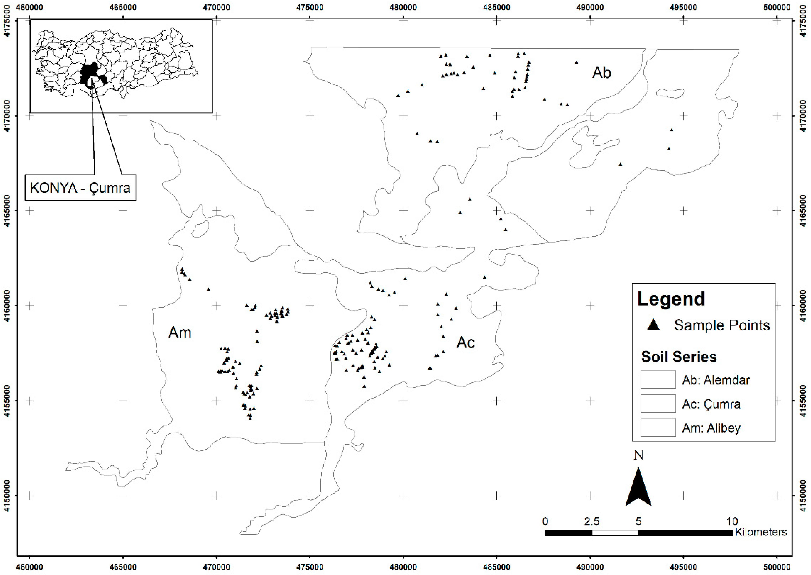
2.1. Study Area and Data

The soil data were collected in Çumra–Konya plain (37°50′54″ N 32°43′03″ E–37°12′17″ N 33°07′16″ E, 1011 m altitude) within an area of about 280,000 ha located 30 km away from the southeast of Konya city. The map is presented for the coordinates of 291 soil samples in the study area (Figure 1). Based on the Köppen–Geiger climate system [35], the climate of the study area is semi-arid with usually cold and snowy winters and hot and dry summers. According to the long-term climate record, the annual average temperature, relative humidity, and precipitation are 11.4 °C, 62.14%, and 296.8 mm, respectively [36]. The soils of the study area are formed by volcanic rocks, marine, and lacustrine deposits [37]. However, they have some restrictive properties such as deep clay texture formed on alluvial parental materials, low organic matter content, high pH value, low aggregate stability, and shallow soil depth [33,38]. Therefore, the region has insufficient drainage and faces soil erosion [39].
All the soil samples were collected from 0–20 cm soil profiles and taken from at least five points in each plot. These five samples were combined to form a representative sample. These samples were air-dried under laboratory conditions, passed through a 2 mm sieve, and thoroughly mixed. Finally, these processed soil samples were stored for laboratory analyses.
Physical and chemical soil properties were measured using relevant standard laboratory analytical methods (Table 1). Based on the results, porosity and effective porosity values were calculated using Equations (1) and (2).
P = ( 1 P b P s ) 10
E P = P F C
where P is porosity (cm3 cm−3), Ps is particle density (g cm−3), Pb is bulk density (g cm−3), EP is effective porosity (cm3 cm−3), and FC is field capacity by volume (cm3 cm−3).
Experimental Ks data was absent in the study area; therefore, the estimation of Ks values was performed by the widely used methods of Saxton and Rawls [12] and Van Genuchten et al. [17]. In the end, the correlation matrix was developed to see the relation between estimated Ks values by the Saxton and Rawls [12], and the Van Genuchten et al. [17] methods, and soil input data (Table 2). Accordingly, the sum of absolute values, except insignificant values of correlation coefficients, was 2.517 for Saxton and Rawls’ [12] method, while that for Van Genuchten et al.’s [17] method was 3.766. Therefore, the result of the latter was selected to evaluate the performance metrics of the machine learning methods.

2.2. Machine Learning Methods

In this study, neural-network-based machine learning methods, artificial neural networks (ANN) and deep learning (DL), and tree-based machine learning methods such as decision tree (DT) and random forest (RF) were employed to estimate the Ks parameter.

2.2.1. Artificial Neural Networks

The artificial neural networks (ANN) algorithm is a mathematical model which is inspired by human nervous systems. This powerful tool can handle and solve complex and difficult problems due to its structure. Artificial neurons are the main units of a neural network that are connected by weights inside the layers. The general working principle of an ANN model is based on training the model first, then validating it for performance evaluation; this process is repeated until an acceptable level of error is encountered. Specifically, each artificial neuron receives a weighted input. These inputs are the outputs of neurons in the previous layer or input variables. After this procedure, the model sums up the inputs and adds a bias term, and then passes the results using an activation function [47]. A typical ANN structure consists of an input layer, one or more hidden layers, and an output layer. The number of hidden layers and neurons increases with the complexity of data.
Several NN types can be used depending on the requirements of the application [48]. The most used are perceptron, feed-forward (FF), convolution, recurrent, Kohonen maps, and support vector machines (SVM). Perceptron is the most basic and smallest NN that performs certain computations to detect features in the input data. Having a simple structure, they are only capable of implementing linearly separable problems. FF NNs on the other hand, find applications in more complex applications such as image processing, computer vision, and speech processing. They can be further classified into single and multi-layered NNs, where the number of layers depends on the complexity. Apart from this flexibility, they can deal with data that contain significant noise and are fast and easy to implement. In contrast, convolution NNs are complex to design and slow in performance depending on the number of hidden layers. For sophisticated applications such as text auto-suggest, grammar checking, text-to-speech, and translation, recurrent NNs are used because they are capable of modeling sequential data. However, training these NNs can be a challenging task. Kohonen maps are used in specialized applications to recognize patterns in the data, for instance in medical analysis to cluster data into different categories. SVMs, which are considered very robust for prediction applications, analyze the data for classification and regression analysis.
The ANN is a well-known and widely adopted method for modeling hydrological studies [49,50]. In particular, the method is used in many studies for the estimation of Ks [6,8,9,10,11,12,13,14,16,17]. In this study, the ANN is implemented as a reference machine learning method to compare the performance metrics of other methods.

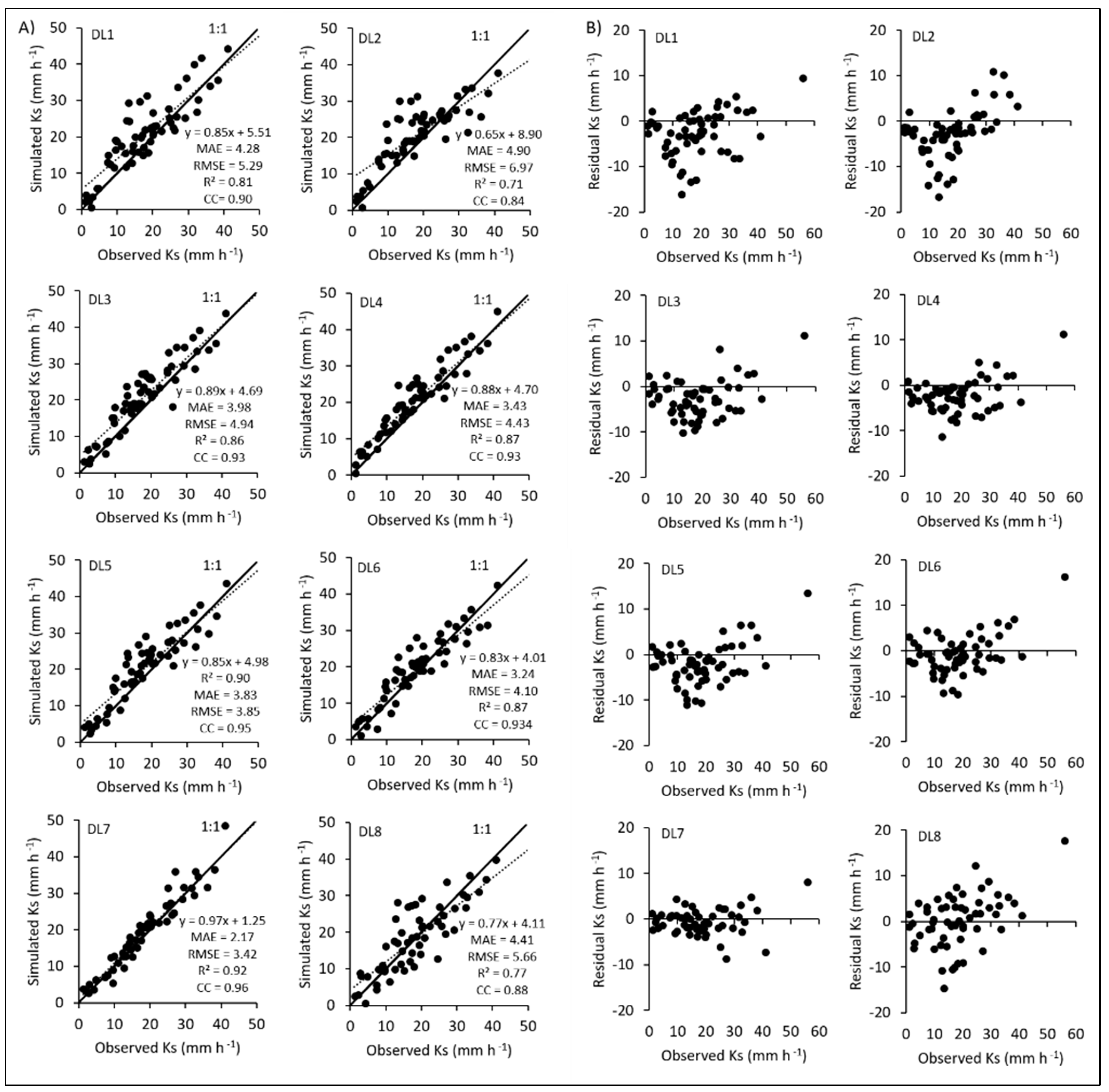
2.2.2. Deep Learning

Due to satisfactory results and great potential, deep learning (DL) was first introduced by Dechter [51] and has been increasingly used for hydrological and agricultural studies over the last years [52,53,54]. DL is an extended version of ANN [55]. The main difference between DL and ANN is that it uses more hidden layers [56]. This feature gives the possibility of higher learning skills and modeling performance, especially for complex datasets. A typical DL structure consists of input, hidden, and output layers.

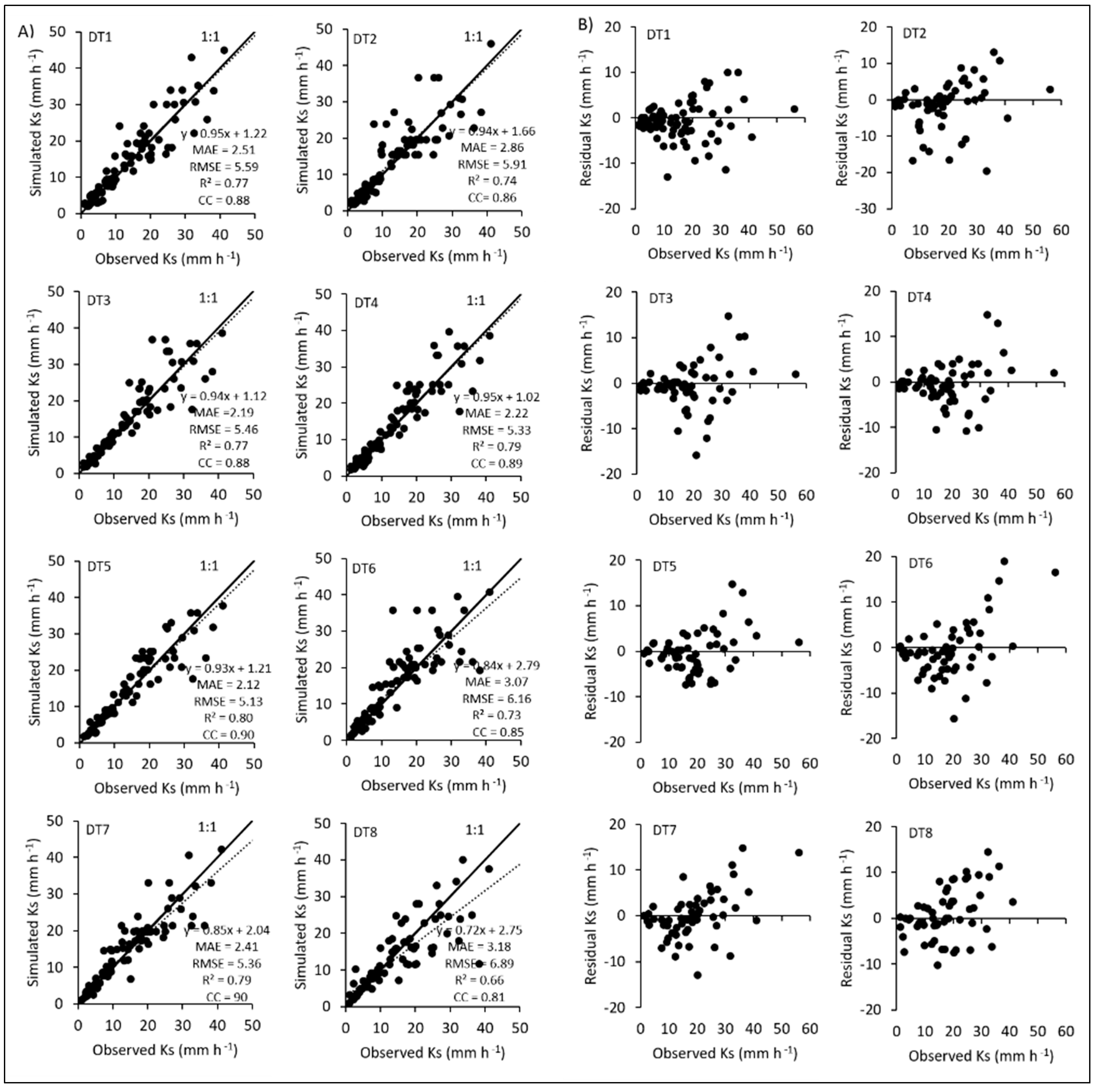
2.2.3. Decision Tree

A decision tree (DT) is one of the widely used methods among machine learning models for solving classification and regression problems. The DT model uses a tree figure to show its correlation with the output data using the observed data in the dataset to be analyzed [57]. The leaves symbolize the output of the model, while the branches symbolize the connection of the input features of the model. One of the most important features of the DT method is to convert complex decision-making problems to simpler and understandable problems by dividing them into a collection of simple decisions [58].

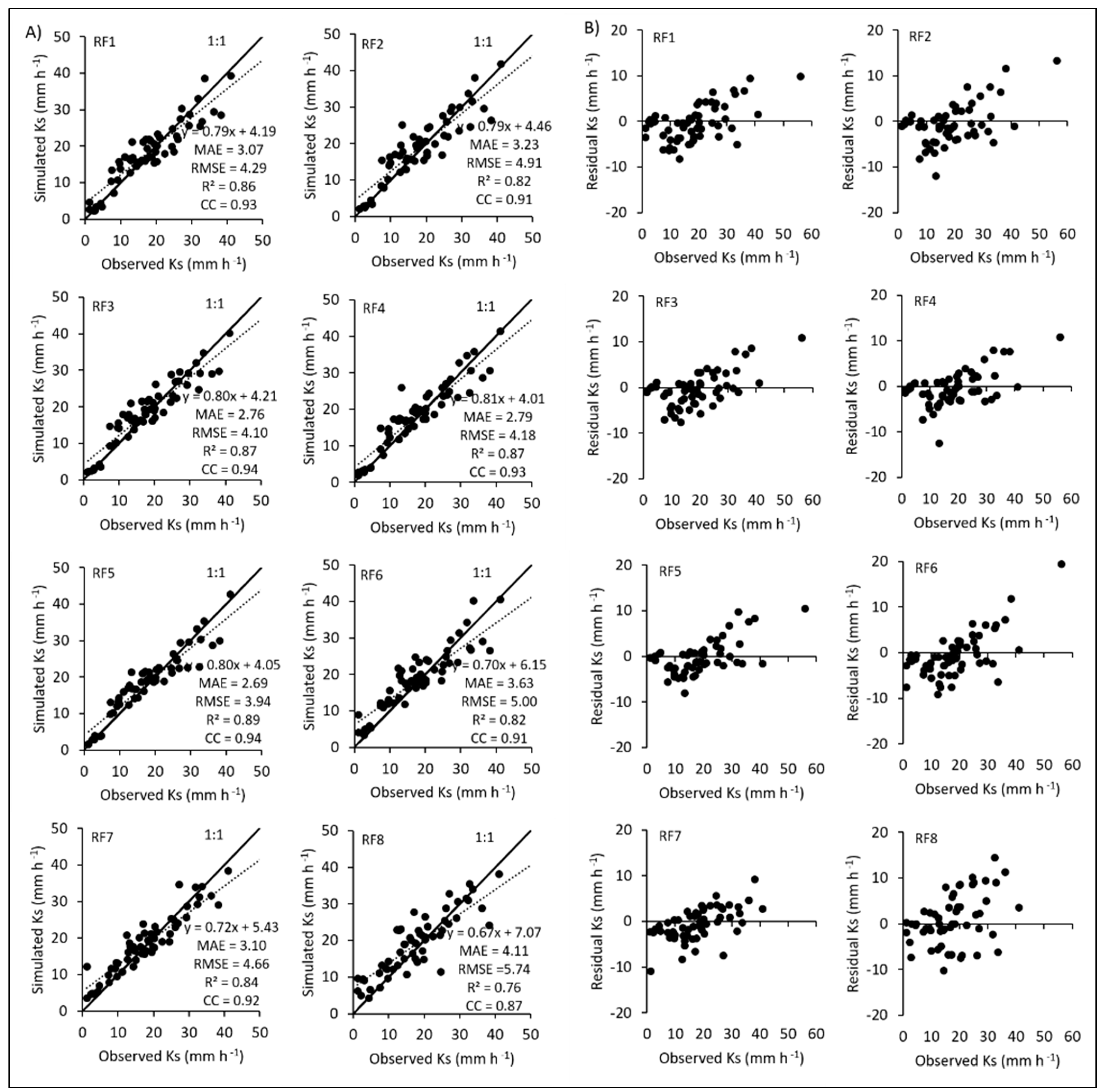
2.2.4. Random Forest

A random forest (RF) is an ensemble model which was developed by Breiman [59] and is used for solving classification and regression problems. It is an improved version of the DT model which consists of multiple decision trees. This improvement is a result of the fact that more trees there are, the more robust the forest [60]. The limitations of DT compared with RF are that the former has overfitting problems since the RF model uses each DT randomly, and the output is an average of the individual DT estimation.

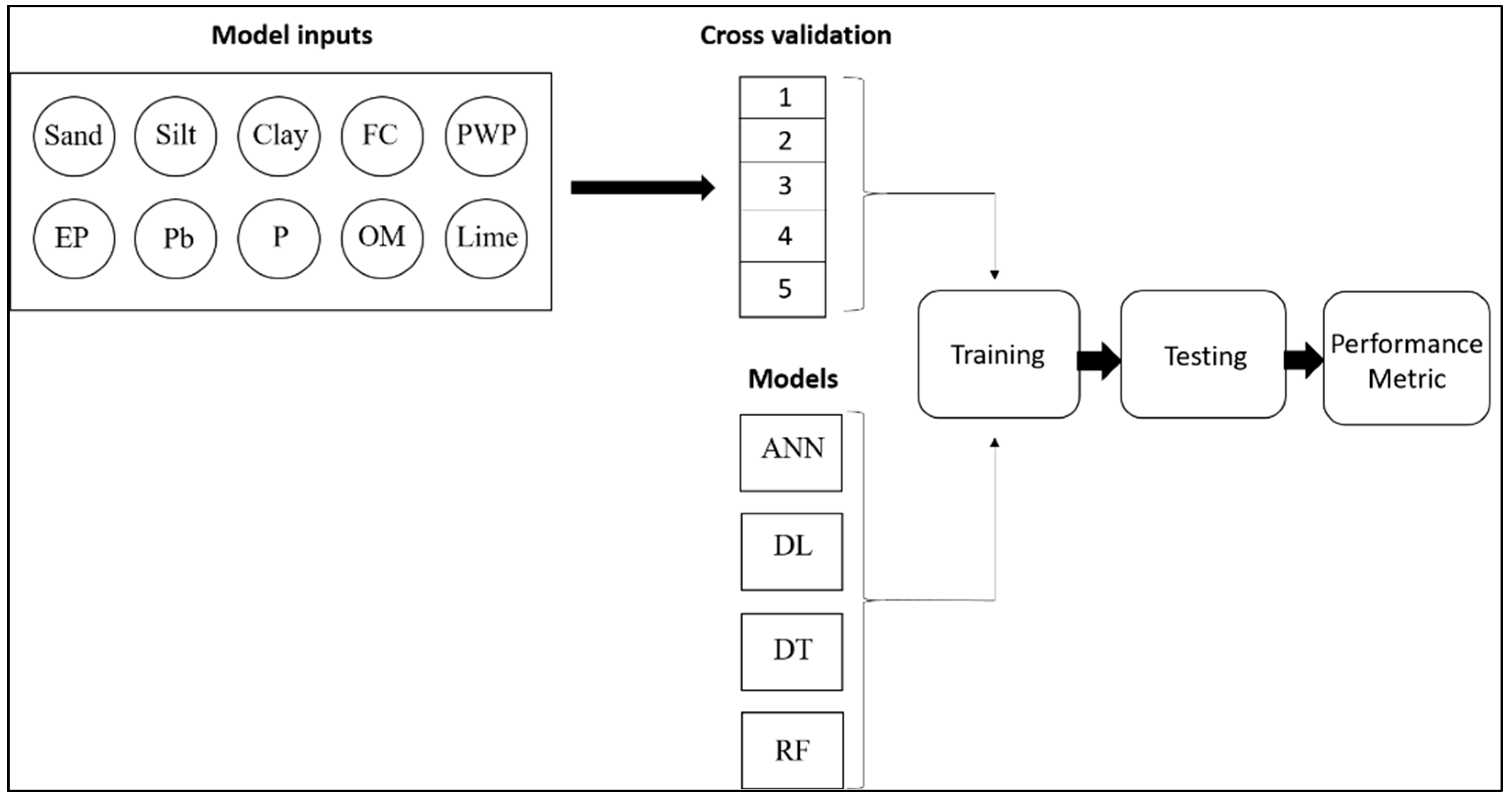
2.3. Selected Inputs and Model Development

The neural-network-based (ANN and DL) and tree-based machine learning methods (DT and RF) were used to simulate the Ks value. To establish the models, soil texture (clay, silt, and sand), effective porosity, bulk density, permanent wilting point, field capacity, lime, organic carbon, and porosity were used as input variables. These input variables are associated with the Ks values of soils, and they have been applied in previous studies for the estimation of Ks [6,8,9,10,11,12,13,14,16,17].
It is well-known that the Ks value interacts with the physical and mechanical properties of the soil. Therefore, the correlation of soil data belonging to this interaction with the Ks value is shown in the correlation matrix and the combinations were developed accordingly (Table 2). Combination 7 consisted of inputs used in the Van Genuchten et al. [17] method, while combination 8 of input was used in the Saxton and Rawls [12] method. In this way, the performance metrics of machine learning methods by using input combinations of these methods could be emulated. The data reduction technique was applied for the development of the combinations, which aimed to take advantage of the available soil feature to estimate the Ks value at a high rate. Effective porosity was added in the first 6 combinations due to the high correlation. Sand and clay contents were taken into consideration in every combination and the effects of other soil mechanical properties were also evaluated respectively. According to this phenomenon, the most relevant input combinations were created to estimate the value of Ks. The combinations of the input variables can be seen in Table 3.
All the datasets were normalized between 0 and 1 for minimizing the incoherency and redundancy of the data using the following equation:
Y n o r m = Y i Y m i n Y m a x Y m i n
where Y n o r m is the normalized data of Y i , Y i is the observed data, Y m a x and Y m i n are the maximum and minimum data, respectively. The observed 291 datasets were employed to estimate the accuracy of the models using k-fold cross-validation, which is more reliable than the train-test split method [56]. In this study, the k value of 5 was used, which means the dataset was separated 5-fold, and models were trained using 4 (k − 1) fold. The trained model was tested on the remaining 1-fold. This procedure was run 5 (k) times, thus repeating the experiments 5 times and the results were averaged (Figure 2). Figure 3 shows a flowchart of the implemented model.

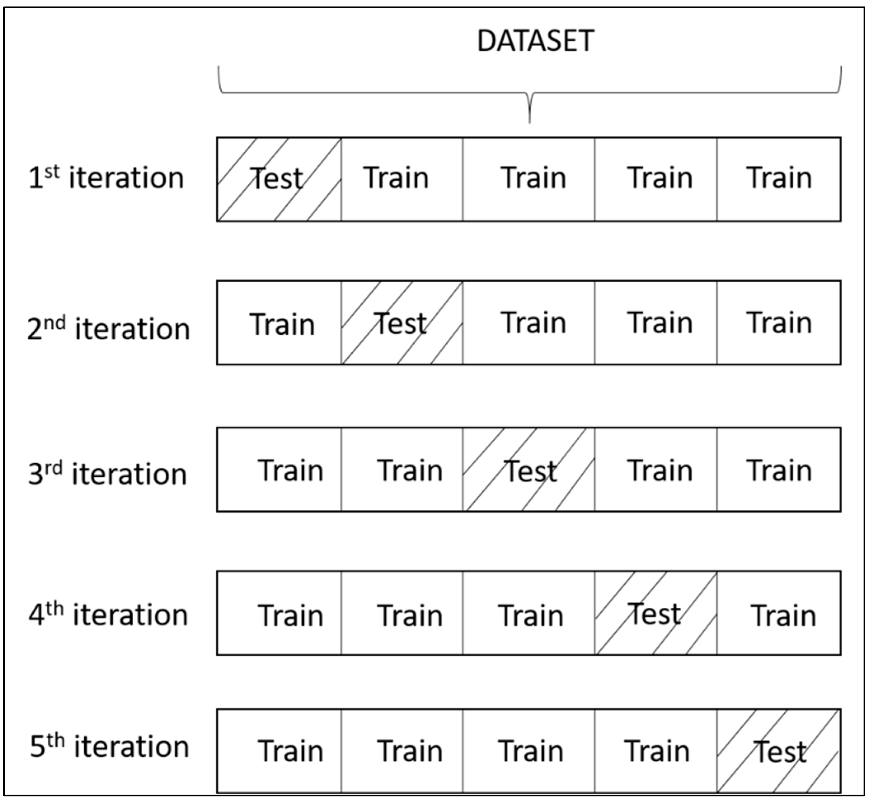
2.4. Performance Evaluation

The performance metrics of the ANN, DL, DT, and RF models were used including mean absolute error (MAE), root means square error (RMSE), coefficient of determination (R2), and correlation coefficient (CC). The calculations of these metrics are shown below:
MAE = | i = 1 n ( Z i Y i ) n |
RMSE = i = 1 n ( Z i Y i ) 2 n
R 2 = 1 i = 1 n [ Y i Z i ] 2 i = 1 n [ Y i   Y ¯ ] 2
CC = i = 1 n ( Y i Y ¯ )   ( Z i Z ¯ ) i = 1 n ( Y i Y ¯ ) 2 i = 1 n ( Z i Z ¯ ) 2
where Z i is the predicted value, and Yi is the observed value. Y ¯ is the mean value of observed values and Z ¯ is the mean value of the predicted values. For the evaluation of the model performance, the high model performance can be confirmed when the RMSE and MAE values are low, and R 2 and CC values are high.

3. Results

3.1. Adjustment of Input Variables

The correlation matrix of the input and output soil variables is presented in Table 2. This matrix helps to develop combinations for the models, as there is no significant relation between aggregate stability and penetration resistance variables with Ks value. Therefore, these two soil input variables were not used in the combinations. However, soil organic carbon, despite having insignificant relation with Ks value, is still used in combination 8 because this combination is used as input variables for Saxton and Rawls [12] equation. The other soil input variables such as sand, silt, clay, field capacity, permanent wilting point, porosity, effective porosity, and lime contents were used for the development of combinations. The findings demonstrated that effective porosity and Ks values (0.788) have the highest correlation among the soil input variables. The second highest correlation of 0.548 was observed between Ks and sand values. The third highest correlation of 0.226 was obtained between Ks and porosity. Among the significant values, other soil input variables such as silt, clay, bulk density, field capacity, permanent wilting point, and lime had a negative correlation with Ks. The statistical values of the soil data can be seen in Table 4. The negative values of skewness were −0.06, −0.06, −0.57, and −0.13 mm h−1 for silt, field capacity, porosity, and effective porosity, and the positive values of kurtosis were 0.12, 0.08, 0.12 and 3.37 mm h−1 for bulk density, porosity, lime, and organic carbon, respectively. The maximum, minimum, mean, and standard deviation values of Ks were 58.91, 0.88, 16.08, and 11.33 mm h−1, respectively. The highest value of variation coefficient was observed for Ks values with 0.66 mm h−1. The highest value of skewness was obtained by Ks value with 0.86 mm h−1 and the lowest value of kurtosis was obtained by an effective porosity value of −0.88.

3.2. Performance of Machine Learning Methods

The performance metrics of four supervised machine learning methods using eight combinations of measured soil input variables are shown in Table 5 and Table 6, and Figure 4 for estimation of Ks. Scatter and residual plots of observed and simulated Ks values are shown in Figure 5, Figure 6, Figure 7 and Figure 8 for the ANN, DL, DT, and RF methods, respectively, for the eight soil input combinations. In general, the highest MAE and RMSE values were observed for the ANN6 method with soil inputs of sand, clay, effective porosity, permanent wilting point, field capacity, bulk density, porosity, and lime contents, and the highest R 2 and CC values were observed for the ANN7 method with soil inputs of sand, silt, clay, permanent wilting point, field capacity, and bulk density. It can be concluded that neural-network-based models (ANN and DL) had the best performance metrics for combination 7 with soil inputs of sand, silt, clay, permanent wilting point, field capacity, and bulk density values, while they had the lowest performance metrics for combination 2 with soil inputs of clay and effective porosity. For tree-based models (DT and RF), the lowest performance was obtained for combination 8 with soil inputs of sand, clay, bulk density, and organic carbon contents, while the best performance was obtained for combination 5 with soil inputs of sand, clay, effective porosity, and bulk density.

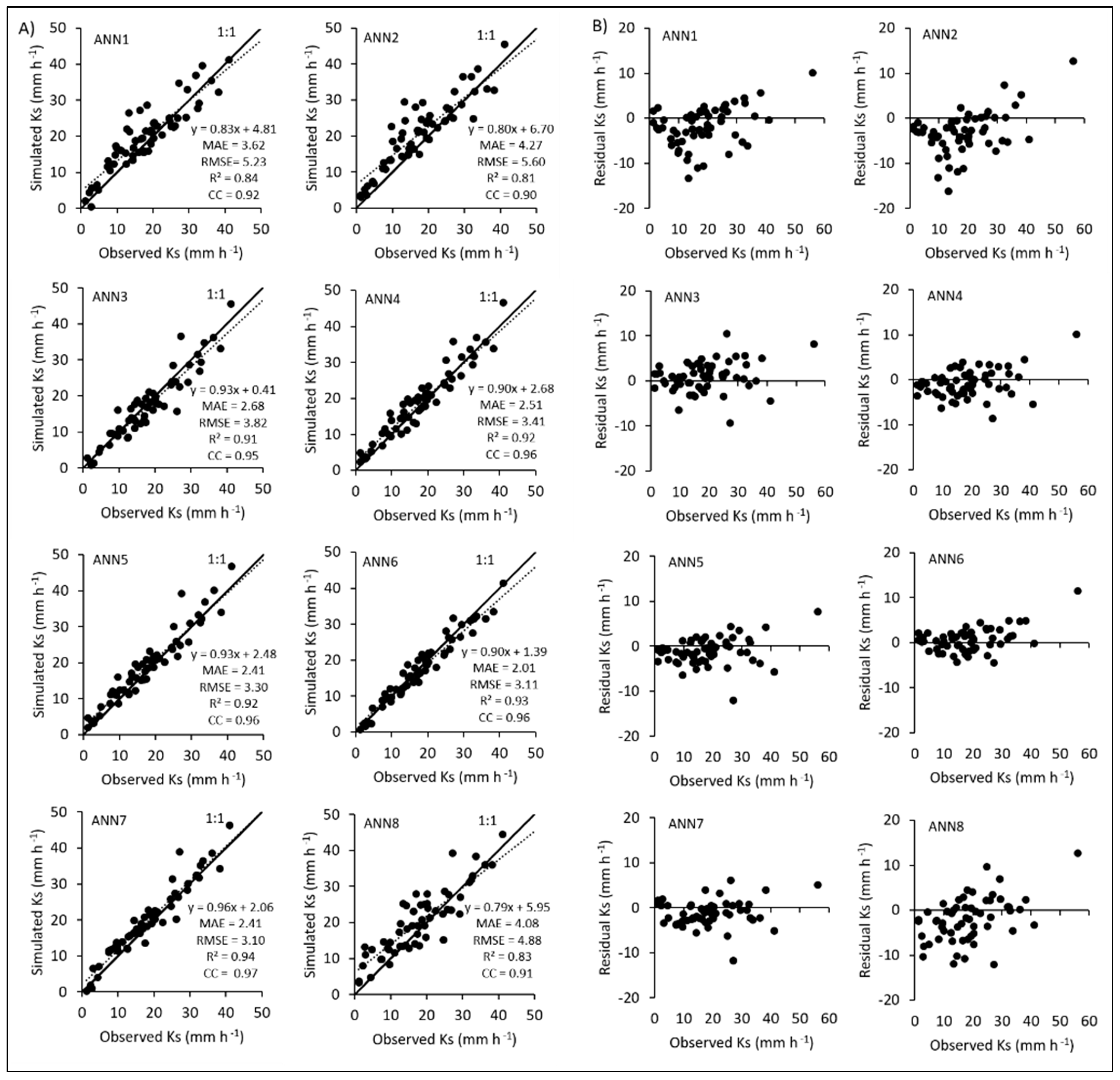
3.3. Performances of Neural-Network-Based Machine Learning Methods

The best performance was observed when the ANN 2(2-3-4-4-8-6-4)-4-1, which means that the algorithm consists of two neurons of combination 1, two neurons of combination 2, three neurons of combination 3, four neurons of combination 4, four neurons of combination 5, eight neurons of combination 6, six neurons of combination 7 and four neurons of combination 8 in input layers, four neurons in the hidden layer and one output layer. The rectified linear unit (ReLU) was employed as the activation function in this study since it is the most used activation function. The ANN7 model fed with soil inputs of sand, silt, clay, permanent wilting point, field capacity, and bulk density demonstrated the highest performance metrics among the other models considering MAE (2.407 mm h−1), RMSE (3.096 mm h−1), R 2 (0.940), and CC (0.970). However, the ANN2 fed with soil inputs of clay and effective porosity had the poorest performance with MAE of 4.272 mm h−1, RMSE of 5.603 mm h−1, R 2 of 0.806, and CC of 0.897. The scatter plots of estimated Ks values by the ANN model with eight soil input combinations are shown in Figure 5A. The data of the scatter plots are generally close to the reference line (1:1) for all combinations. However, the combinations of 1, 2, and 8 for the ANN model showed more scattered points than combinations of 3, 4, 5, 6, and 7. The residual plots of estimated Ks values by the ANN model with eight soil input combinations are shown in Figure 5B. The residual plot demonstrated that the most errors occurred in combination 8, while the least error occurred in combination 6 for the ANN model.
The best accuracy of the Ks value was observed when two hidden layers (50-50) and ReLU were used for the DL model in this study. As can be seen in Table 5, it is seen that the DL model produces the lowest performance for combination 2 with MAE, RMSE, R 2 , and CC equal to 4.898, 6.965, 0.707, and 0.840. The combination of DL7 with soil inputs of sand, silt, clay, field capacity, permanent wilting point, and bulk density showed the best performance with MAE of 2.167 mm h−1, RMSE of 3.423 mm h−1, R 2 of 0.919, and CC of 0.959. The scatter plots of estimated Ks values by the DL model with eight soil input combinations are shown in Figure 6A. From the figure, it can be seen that combinations 2 and 8 had more scattered points than other combinations. The least scattered points were observed for the combination of 7. The residual plots of estimated Ks values by the DL model with eight soil input combinations are shown in Figure 6B. The least residual errors were observed for the combination of 7, while the most residual errors were observed for the combination 8 for the DL model.

3.4. Performances of Tree-Based Machine Learning Methods

The lowest performance was obtained for the DT8 fed with soil inputs of sand, clay, bulk density, and organic carbon contents considering MAE (3.179 mm h−1), RMSE (5.736 mm h−1), R 2 (0.887), CC (0.942). The performance metrics improved significantly when adding organic carbon instead of bulk density values from the soil inputs. In that case, the highest performance was observed for the fifth combination with MAE of 2.121 mm h−1, RMSE of 5.130 mm h−1, R 2 of 0.804, and CC of 0.896. Similar performances were obtained for combination 1 and 3 and also for combinations 4 and 7. The scatter plots of estimated Ks values by the DT model with eight soil input combinations are shown in Figure 7A. It can be noticed that the combinations of the DT model were more scattered than the combinations of the ANN, DL, and RF models. The residual plots of estimated Ks values by the DT model with eight soil input combinations are shown in Figure 7B. The highest residual Ks values were observed in combination 6 with the value of 18.60 mm h−1. The least residual errors occurred in combination 5 for the DT model.
The RF model observed the best performance when the number of trees was fixed to 10. The model gave the poorest performance for combination 8 with MAE of 4.106 mm h−1, RMSE of 5.736 mm h−1, R 2 of 0.755, and CC of 0.869. The performance of the RF model improved when adding organic carbon instead of bulk density from the soil inputs. The performance metrics demonstrated similar performance to the RF model for the third, fourth, and fifth input combinations. The best performance was observed for the RF5 model with soil inputs of sand, clay, effective porosity, and bulk density with MAE of 2.685 mm h−1, RMSE of 3.936 mm h−1, R 2 of 0.887, and CC of 0.942. The scatter plots of estimated Ks values by the RF model with eight soil input combinations are shown in Figure 8A. The most scattered points were obtained from combination 8, while the least scattered points were obtained from combination 7 for the RF model. The residual plots of estimated Ks values by the RF model with eight soil input combinations are shown in Figure 8B. According to the figure, similar residual errors were observed for the combination of 3, 4, and 5. However, among them, the least residual errors occurred in combination 5 for the RF model.

4. Discussion

The present study evaluated neural-network-based (ANN and DL) and tree-based (DT and RF) models with different combinations of soil input variables based on the van Genuchten formula in the semi-arid environment. Zhang and Schaap [2] suggested in their studies that new statistical methods should be employed using relevant and good-quality data for the estimation of Ks. In this study, the results indicated that all the machine learning methods used have a satisfactory correlation between Ks and soil input variables. Due to solving complex and nonlinear features, machine learning methods can simulate the complicated process of soil nature because these methods do not need to know the characteristic of the implemented variables [61].
Another aim of this study was to estimate the Ks values with the least input combinations ensuring high accuracy. For this purpose, eight combinations were developed using ANN, DL, DT, and RF models to evaluate the estimation of Ks value. Accordingly, the first six combinations included effective porosity to see the performances of the models, since it has the highest impact on soil water transmission and correlates to the selected soil properties, except for penetration resistance and organic carbon. The first three combinations are developed based on clay and sand from the soil texture, as it is known that sand and clay contents are one of the most important factors that directly affect the Ks in soil [62,63,64]. When the soil contains a high amount of sand, the Ks are increased. On the contrary, when the soil contains a high amount of clay, the Ks are decreased. This finding is in agreement with Table 2. It can be seen that the performance metrics of the first three combinations have similar results since the use of clay and sand contents together offer high accuracy to the models. It has been stated in many studies that the field capacity is used in the estimation of Ks [12,65,66]. However, the field capacity does not have a direct impact on the estimation of Ks and therefore does not impact the result significantly. Since bulk density is an indicator of soil compaction, it impacted positively on the estimation of Ks. The compression of the pores starts from the effective porosity and progresses towards the micropores [14]. With the decrease of effective porosity, infiltration is decreased, and runoff is increased. Finally, bulk density increases. In this respect, in five combinations, the soil textures and bulk density have a high impact on machine learning methods for the estimation of Ks. Lime content and porosity are calculated by bulk density in this study. Therefore, the combination which was developed from these two soil parameters does not impact the estimation of Ks values. The previous study conducted in this study area showed that soil lime content plays a key role in water retention up to certain levels, but this efficiency decreases due to rising lime content [67]. The decrease in the disclosure rate in combination 8 is explained by the organic carbon value not being correlated with Ks values. When many studies are examined, it is seen that the organic carbon value affects the water movement of the soils. However, in this study, it is seen in the correlation matrix values that it has no effect, since the organic carbon in the soils of the study area is very low with an average of 0.85 and the variability in the carbon value is limited.
The performance metrics demonstrated that the ANN was superior to the DL method in all soil input combinations for the neural-network-based models. This finding can be explained by the fact that the DL method requires more experimental data for boosting its modeling performance. A similar explanation was pointed out also by Kamilaris and Prenafeta-Boldú [53] who indicated that the usage of the DL method has recently increased in soil science due to its ability to solve complicated datasets. The performance metrics showed that the RF model was a better result than the DT model in all soil input combinations for the tree-based models. RF is an improved version of the DT model since it boosts the robustness of the classification feature. However, the RF is known as a black-box model and therefore it is less explicable than the DT model, but it is seen that the RF models demonstrate better performance and stability than the estimation in previous studies.
The RF model with combination 5 had the highest performance among the tree-based models, while the ANN model with combination 7 had the highest performance among the neural-network-based models. It can be seen from Table 3 that combination 5 had four input parameters but combination 7 had six input parameters. This can be explained by the fact that the ANN model had a much more complicated architecture than the RF model, which allowed for boosting its modeling performance with more input variables.
In general, the ANN model demonstrated better performance metrics compared to other models. This observation is in agreement with the results of [68] who reported that the ANN model shows satisfactory results for the estimation of Ks. Similarly, [69] indicated that the ANN demonstrates good performance for the estimation of Ks.

5. Conclusions

Soil hydraulic conductivity is a fundamental parameter for the estimation of water balance at regional and global levels and the determination of groundwater recharge in the vadose zone. In recent years, mathematical methods have been applied frequently by using soil features to obtain Ks. This study demonstrated that the machine learning methods can be an alternative way to overcome these challenges.
The comparison analysis of neural-network-based models (ANN and DL) and tree-based models (DT and RF) models was evaluated based on the van Genuchten equation under eight combinations of soil input data. The reason for using two group of machine learning methods is to find out the best category. In general, all the machine learning methods had satisfactory performance for estimation of Ks. Among the categories, the neural-network-based models (ANN and DL) had better performance than tree-based models (DT and RF). The overall results showed that the ANN method with sand, silt, clay, field capacity, permanent wilting point, and bulk density (ANN7) had the best performance among the other methods. The RF method with sand, clay, effective porosity, and bulk density (RF5) had the best performance among the tree-based models. These findings demonstrate that the ANN method is more applicable to the study area. Likewise, the ANN method can figure out a much more complex dataset to estimate Ks for calcareous alluvial soils in a semi-arid region. In the case of the input data, it was observed that soil texture, bulk density, and effective porosity variables have a great impact on estimating the Ks value since soil properties, such as lime penetration resistance, aggregate stability, and porosity, have a low impact on the estimation of Ks. These findings are important to understand the impact of soil parameters in a study area for estimating the Ks value.
Lastly, further studies should collect more data for enhancing modeling performance. Likewise, the machine learning methods should be tested under different environmental conditions, which means seeing the performance metrics of different specific soil input combinations for the study area. This is particularly important to see the adaptation of new statistical methods such as machine learning.

Author Contributions

Supervision, S.S.Y.; conceptualization, S.S.Y. and G.A.; methodology, S.S.Y., G.A., H.N. and C.Ş.; software, A.M.M.; validation, G.A., A.M.M., B.K. and M.T.; formal analysis, S.S.Y., A.M.M. and G.A.; investigation, S.S.Y., H.N. and C.Ş.; resources, S.S.Y., H.N. and C.Ş.; data curation, G.A., A.M.M., B.K. and M.T.; writing—original draft preparation, S.S.Y. and G.A.; writing—review and editing, H.N., C.Ş., A.M.M., B.K. and M.T.; visualization, G.A., M.T. and B.K.; project administration, S.S.Y., H.N. and C.Ş. All authors have read and agreed to the published version of the manuscript.

Funding

This research was funded by the Deanship of Scientific Research, the Vice Presidency for Graduate Studies and Scientific Research, King Faisal University, Saudi Arabia (Grant No. 2010), through its KFU Research Summer initiative.

Data Availability Statement

Not applicable.

Acknowledgments

The authors gratefully acknowledge TÜBİTAK for this research prepared from data of the TÜBİTAK via project no 112O314.

Conflicts of Interest

The authors declare no conflict of interest.

References

  1. Stenitzer, E.; Diestel, H.; Zenker, T.; Schwartengräber, R. Assessment of Capillary Rise from Shallow Groundwater by the Simulation Model SIMWASER Using Either Estimated Pedotransfer Functions or Measured Hydraulic Parameters. Water Resour. Manag. 2007, 21, 1567–1584. [Google Scholar] [CrossRef]
  2. Zhang, Y.; Schaap, M.G. Estimation of saturated hydraulic conductivity with pedotransfer functions: A review. J. Hydrol. 2019, 575, 1011–1030. [Google Scholar] [CrossRef]
  3. Ghosh, B.; Pekkat, S. An Appraisal on the Interpolation Methods Used for Predicting Spatial Variability of Field Hydraulic Conductivity. Water Resour. Manag. 2019, 33, 2175–2190. [Google Scholar] [CrossRef]
  4. Tayfur, G.; Nadiri, A.A.; Moghaddam, A.A. Supervised Intelligent Committee Machine Method for Hydraulic Conductivity Estimation. Water Resour. Manag. 2014, 28, 1173–1184. [Google Scholar] [CrossRef] [Green Version]
  5. Tzimopoulos, C.D.; Sakellariou-Makrantonaki, M. A new analytical model to predict the hydraulic conductivity of unsaturated soils. Water Resour. Manag. 1996, 10, 397–414. [Google Scholar] [CrossRef]
  6. van Genuchten, M.T. A Closed-form Equation for Predicting the Hydraulic Conductivity of Unsaturated Soils. Soil Sci. Soc. Am. J. 1980, 44, 892–898. [Google Scholar] [CrossRef] [Green Version]
  7. Brooks, R.H.; Corey, A.T. Hydraulic properties of porous media and their relation to drainage design. Trans. ASAE 1964, 7, 26–28. [Google Scholar]
  8. Rawls, J.W.; Gimenez, D.; Grossman, R. Use of soil texture, bulk density, and slope of the water retention curve to predict saturated hydraulic conductivity. Trans. ASAE 1998, 41, 983–988. [Google Scholar] [CrossRef]
  9. Mermoud, A.; Xu, D. Comparative analysis of three methods to generate soil hydraulic functions. Soil Tillage Res. 2006, 87, 89–100. [Google Scholar] [CrossRef]
  10. Rawls, W.J.; Brakensiek, D.L. Estimation of Soil Water Retention and Hydraulic Properties. In Unsaturated Flow in Hydrologic Modeling: Theory and Practice; Morel-Seytoux, H.J., Ed.; Springer: Dordrecht, The Netherlands, 1989; pp. 275–300. [Google Scholar] [CrossRef]
  11. Saxton, K.E. Estimating Generalized Soil-water Characteristics from Texture. Soil Sci. Soc. Am. J. 1986, 50, 1031–1036. [Google Scholar] [CrossRef]
  12. Saxton, K.E.; Rawls, W.J. Soil Water Characteristic Estimates by Texture and Organic Matter for Hydrologic Solutions. Soil Sci. Soc. Am. J. 2006, 70, 1569–1578. [Google Scholar] [CrossRef] [Green Version]
  13. Wagner, B.; Tarnawski, V.R.; Stöckl, M. Evaluation of pedotransfer functions predicting hydraulic properties of soils and deeper sediments. J. Plant Nutr. Soil Sci. 2004, 167, 236–245. [Google Scholar] [CrossRef]
  14. Ahuja, L.R.; Naney, J.W.; Green, R.E.; Nielsen, D.R. Macroporosity to Characterize Spatial Variability of Hydraulic Conductivity and Effects of Land Management. Soil Sci. Soc. Am. 1984, 48, 699–702. [Google Scholar] [CrossRef]
  15. Bourazanis, G.; Katsileros, A.; Kosmas, C.; Kerkides, P. The effect of treated municipal wastewater and fresh water on saturated hydraulic conductivity of a clay-loamy soil. Water Resour. Manag. 2016, 30, 2867–2880. [Google Scholar] [CrossRef]
  16. Cosby, B.J.; Hornberger, G.M.; Clapp, R.B.; Ginn, T.R. A Statistical Exploration of the Relationships of Soil Moisture Characteristics to the Physical Properties of Soils. Water Resour. Res. 1984, 20, 682–690. [Google Scholar] [CrossRef] [Green Version]
  17. Van Genuchten, M.; Leij, F.; Yates, S. The RETC Code for Quantifying the Hydraulic Functions of Unsaturated Soils; US Salinity Laboratory US Department of Agriculture, Agricultural Research Service: Riverside, CA, USA, 1991. [Google Scholar]
  18. Klopp, H.W.; Arriaga, F.A.; Daigh, A.L.M.; Bleam, W.F. Development of functions to predict soil hydraulic properties that account for solution sodicity and salinity. Catena 2021, 204, 105389. [Google Scholar] [CrossRef]
  19. Minasny, B.; Hopmans, J.W.; Harter, T.; Eching, S.O.; Tuli, A.; Denton, M.A. Neural Networks Prediction of Soil Hydraulic Functions for Alluvial Soils Using Multistep Outflow Data. Soil Sci. Soc. Am. J. 2004, 68, 417–429. [Google Scholar] [CrossRef]
  20. Rogiers, B.; Mallants, D.; Batelaan, O.; Gedeon, M.; Huysmans, M.; Dassargues, A. Estimation of Hydraulic Conductivity and Its Uncertainty from Grain-Size Data Using GLUE and Artificial Neural Networks. Math. Geosci. 2012, 44, 739–763. [Google Scholar] [CrossRef] [Green Version]
  21. Zuo, Y.; He, K. Evaluation and Development of Pedo-Transfer Functions for Predicting Soil Saturated Hydraulic Conductivity in the Alpine Frigid Hilly Region of Qinghai Province. Agronomy 2021, 11, 1581. [Google Scholar] [CrossRef]
  22. Araya, S.N.; Ghezzehei, T.A. Using Machine Learning for Prediction of Saturated Hydraulic Conductivity and Its Sensitivity to Soil Structural Perturbations. Water Resour. Res. 2019, 55, 5715–5737. [Google Scholar] [CrossRef]
  23. Naganna, S.R.; Deka, P.C. Artificial intelligence approaches for spatial modeling of streambed hydraulic conductivity. Acta Geophys. 2019, 67, 891–903. [Google Scholar] [CrossRef]
  24. Sihag, P.; Esmaeilbeiki, F.; Singh, B.; Ebtehaj, I.; Bonakdari, H. Modeling unsaturated hydraulic conductivity by hybrid soft computing techniques. Soft Comput. 2019, 23, 12897–12910. [Google Scholar] [CrossRef]
  25. Kashani, H.M.; Ghorbani, M.A.; Shahabi, M.; Naganna, S.R.; Diop, L. Multiple AI model integration strategy—Application to saturated hydraulic conductivity prediction from easily available soil properties. Soil Tillage Res. 2020, 196, 104449. [Google Scholar] [CrossRef]
  26. Kalumba, M.; Bamps, B.; Nyambe, I.; Dondeyne, S.; van Orshoven, J. Development and functional evaluation of pedotransfer functions for soil hydraulic properties for the Zambezi River Basin. Eur. J. Soil Sci. 2021, 72, 1559–1574. [Google Scholar] [CrossRef]
  27. Morshedi, A.; Sameni, A.M. Hydraulic conductivity of calcareous soils as affected by salinity and sodicity. I. Effect of concentration and composition of leaching solution and type and amount of clay minerals of tested soils. Commun. Soil Sci. Plant Anal. 2000, 31, 51–67. [Google Scholar] [CrossRef]
  28. Amer, A.M.M.; Logsdon, S.D.; Davis, D. Prediction of hydraulic conductivity as related to pore size distribution in unsaturated soils. Soil Sci. 2009, 174, 508–515. [Google Scholar] [CrossRef] [Green Version]
  29. Fernández-Ugalde, O.; Virto, I.; Bescansa, P.; Imaz, M.J.; Enrique, A.; Karlen, D.L. No-tillage improvement of soil physical quality in calcareous, degradation-prone, semiarid soils. Soil Tillage Res. 2009, 106, 29–35. [Google Scholar] [CrossRef]
  30. Khodaverdiloo, H.; Homaee, M.; van Genuchten, M.T.; Dashtaki, S.G. Deriving and validating pedotransfer functions for some calcareous soils. J. Hydrol. 2011, 399, 93–99. [Google Scholar] [CrossRef]
  31. Kabir, E.B.; Bashari, H.; Bassiri, M.; Mosaddeghi, M.R. Effects of land-use/cover change on soil hydraulic properties and pore characteristics in a semi-arid region of central Iran. Soil Tillage Res. 2020, 197, 104478. [Google Scholar] [CrossRef]
  32. Mozaffari, H.; Moosavi, A.A.; Sepaskhah, A.R. Land use-dependent variation of near-saturated and saturated hydraulic properties in calcareous soils. Environ. Earth Sci. 2021, 80, 769. [Google Scholar] [CrossRef]
  33. Şeker, C.; Özaytekin, H.H.; Gümüş, İ.; Karaarslan, E.; Ummahan, K. Çumra Ovasında Önemli ve Yaygın Üç Toprak Serisinin Toprak Kalite İndislerinin Belirlenmesi, Proje Raporu; Proje No: 112O314; Program Kodu: Konya, Turkey, 2016. (In Turkish) [Google Scholar]
  34. Yamaç, S.S.; Şeker, C.; Negiş, H. Evaluation of machine learning methods to predict soil moisture constants with different combinations of soil input data for calcareous soils in a semi arid area. Agric. Water Manag. 2020, 234, 106121. [Google Scholar] [CrossRef]
  35. Kottek, M.; Grieser, J.; Beck, C.; Rudolf, B.; Rubel, F. World map of the Köppen-Geiger climate classification updated. Meteorol. Z. 2006, 15, 259–263. [Google Scholar] [CrossRef] [PubMed]
  36. MGM. Meteoroloji Genel Müdürlüğü. 2015. Available online: https://www.mgm.gov.tr/ (accessed on 15 October 2022).
  37. Bahçeci, İ.; Dinç, N.; Tarı, A.F.; Ağar, A.İ.; Sönmez, B. Water and salt balance studies, using SaltMod, to improve subsurface drainage design in the Konya–Çumra Plain, Turkey. Agric. Water Manag. 2006, 85, 261–271. [Google Scholar] [CrossRef]
  38. Driessen, P.M.; Meester, T.D. Soils of the Çumra Area, Turkey; Pudoc: Wageningen, The Netherlands, 1969. [Google Scholar]
  39. Topraksu. Konya Kapalı Havzası Toprakları; Toprak Etüdleri ve Haritalama Dairesi Topak Etüdleri Fen Heyeti Md; Ankara Yayın: Ankara, Turkeys, 1978; p. 288. [Google Scholar]
  40. Gee, G.W.; Bauder, J.; Klute, A. Methods of Soil Analysis, Part 1, Physical and Mineralogical Methods; Soil Science Society of America Book Series; American Society of Agronomy, Inc. and Soil Science Society of America, Inc.: Madison, WI, USA, 1986; pp. 383–411. [Google Scholar]
  41. Blake, G.R.; Hartge, K.H. Bulk density. In Methods of Soil Analysis, Part 1-Physical and Mineralogical Methods, 2nd ed.; Klute, A., Ed.; Agronomy Monograph 9; American Society of Agronomy-Soil Science Society of America: Madison, WI, USA, 1986; Volume 9, pp. 363–382. [Google Scholar]
  42. Blake, G.R.; Hartge, K.H. Particle density. In Methods of Soil Analysis, Part 1-Physical and Mineralogical Methods, 2nd ed.; Klute, A., Ed.; Agronomy Monograph 9; American Society of Agronomy-Soil Science Society of America: Madison, WI, USA, 1986; Volume 9, pp. 377–382. [Google Scholar]
  43. Cassel, D.K.; Nielsen, D.R. Field Capacity and Available Water Capacity. In Methods of Soil Analysis; AWE International: Dorset, UK, 1986; pp. 901–926. [Google Scholar] [CrossRef]
  44. Moebius-Clune, B.; Moebius-Clune, D.; Gugino, B.; Idowu, O.; Schindelbeck, R.; Ristow, A.; van Es, H.; Thies, J.; Shayler, H.; McBride, M.; et al. Comprehensive Assessment of Soil Health—The Cornell Framework, 3.2 ed.; Cornell University: Ithaca, NY, USA, 2016. [Google Scholar]
  45. Mclean, E.O. Soil pH and Lime Requirement. In Methods of Soil Analysis; AWE International: Dorset, UK, 1983; pp. 199–224. [Google Scholar] [CrossRef]
  46. Wright, A.F.; Bailey, J.S. Organic carbon, total carbon, and total nitrogen determinations in soils of variable calcium carbonate contents using a Leco CN-2000 dry combustion analyzer. Commun. Soil Sci. Plant. Anal. 2001, 32, 3243–3258. [Google Scholar] [CrossRef]
  47. Ferreira, L.B.; da Cunha, F.F.; de Oliveira, R.A.; Fernandes Filho, E.I. Estimation of reference evapotranspiration in Brazil with limited meteorological data using ANN and SVM—A new approach. J. Hydrol. 2019, 572, 556–570. [Google Scholar] [CrossRef]
  48. Gurney, K. An Introduction to Neural Networks; CRC Press: Boca Raton, FL, USA, 2018. [Google Scholar]
  49. Reis, M.M.; da Silva, A.J.; Zullo Junior, J.; Tuffi Santos, L.D.; Azevedo, A.M.; Lopes, É.M.G. Empirical and learning machine approaches to estimating reference evapotranspiration based on temperature data. Comput. Electron. Agric. 2019, 165, 104937. [Google Scholar] [CrossRef]
  50. Yamaç, S.S. Reference evapotranspiration estimation with kNN and ANN models using different climate input combinations in the semi-arid environment. J. Agric. Sci. 2021, 27, 129–137. [Google Scholar]
  51. Dechter, R. Learning while searching in constraint-satisfaction problems. In Proceedings of the fifth National Conference on Artificial Intelligence (AAAI-86), Philadelphia, PA, USA, 11–15 August 1986; pp. 178–185. [Google Scholar]
  52. de Lucas, P.O.E.; Alves, M.A.; de Silva, P.C.L.E.; Guimarães, F.G. Reference evapotranspiration time series forecasting with ensemble of convolutional neural networks. Comput. Electron. Agric. 2020, 177, 105700. [Google Scholar] [CrossRef]
  53. Kamilaris, A.; Prenafeta-Boldú, F.X. Deep learning in agriculture: A survey. Comput. Electron. Agric. 2018, 147, 70–90. [Google Scholar] [CrossRef]
  54. Saggi, M.K.; Jain, S. Reference evapotranspiration estimation and modeling of the Punjab Northern India using deep learning. Comput. Electron. Agric. 2019, 156, 387–398. [Google Scholar] [CrossRef]
  55. LeCun, Y.; Bengio, Y.; Hinton, G. Deep learning. Nature 2015, 521, 436–444. [Google Scholar] [CrossRef] [PubMed]
  56. Özgür, A.; Yamaç, S.S. Modelling of Daily Reference Evapotranspiration Using Deep Neural Network in Different Climates. arXiv 2020, arXiv:abs/200601760. Available online: https://arxivorg/abs/200601760 (accessed on 15 October 2022).
  57. Liu, S.; McGree, J.; Ge, Z.; Xie, Y. 2—Classification methods. In Computational and Statistical Methods for Analysing Big Data with Applications; Liu, S., McGree, J., Ge, Z., Xie, Y., Eds.; Academic Press: Cambridge, MA, USA, 2016. [Google Scholar]
  58. Safavian, S.R.; Landgrebe, D. A survey of decision tree classifier methodology. IEEE Trans. Syst. Man. Cybern. 1991, 21, 660–674. [Google Scholar] [CrossRef] [Green Version]
  59. Breiman, L. Random Forests. Mach. Learn. 2001, 45, 5–32. [Google Scholar] [CrossRef] [Green Version]
  60. Yamaç, S.S. Artificial intelligence methods reliably predict crop evapotranspiration with different combinations of meteorological data for sugar beet in a semiarid area. Agric. Water Manag. 2021, 254, 106968. [Google Scholar] [CrossRef]
  61. Gocić, M.; Motamedi, S.; Shamshirband, S.; Petković, D.; Ch, S.; Hashim, R.; Arif, M. Soft computing approaches for forecasting reference evapotranspiration. Comput. Electron. Agric. 2015, 113, 164–173. [Google Scholar] [CrossRef]
  62. Arya, L.M.; Leij, F.J.; Shouse, P.J.; van Genuchten, M.T. Relationship between the hydraulic conductivity function and the particle-size distribution. Soil Sci. Soc. Am. 1999, 67, 373. [Google Scholar] [CrossRef]
  63. Frenkel, H.; Levy, G.; Fey, M. Clay dispersion and hydraulic conductivity of clay-sand mixtures as affected by the addition of various anions. Clays Clay 1992, 40, 515–521. [Google Scholar] [CrossRef]
  64. Park, E.-J.; Smucker, A.J.M. Saturated Hydraulic Conductivity and Porosity within Macroaggregates Modified by Tillage. Soil Sci. Soc. Am. J. 2005, 69, 38–45. [Google Scholar] [CrossRef]
  65. Lu, J. Chapter 6—Identification of Forensic Information from Existing Conventional Site-Investigation Data. In Introduction to Environmental Forensics, 3rd ed.; Murphy, B.L., Morrison, R.D., Eds.; Academic Press: San Diego, CA, USA, 2015; pp. 149–164. [Google Scholar] [CrossRef]
  66. Shaykewich, C.F.; Zwarich, M.A. Relationships between soil physical constants and soil physical components of some manitoba soils. Can. J. Soil Sci. 1968, 48, 199–204. [Google Scholar] [CrossRef]
  67. Abdulwahhab, Q. Determination of the Effects of Lime, Organic Matter and Soil Compaction on Some Hydrodynamic Properties of Different Textured Soils. Ph.D. Thesis, Department of Soil Science and Plant Nutrition, Institute of Science, Selcuk University, Konya, Turkey, 2020. [Google Scholar]
  68. Agyare, W.A.; Park, S.J.; Vlek, P.L.G. Artificial Neural Network Estimation of Saturated Hydraulic ConductivityAll rights reserved. No part of this periodical may be reproduced or transmitted in any form or by any means, electronic or mechanical, including photocopying, recording, or any information storage and retrieval system, without permission in writing from the publisher. Vadose Zone J. 2007, 6, 423–431. [Google Scholar] [CrossRef] [Green Version]
  69. Parasuraman, K.; Elshorbagy, A.; Si, B.C. Estimating Saturated Hydraulic Conductivity In Spatially Variable Fields Using Neural Network Ensembles. Soil Sci. Soc. Am. J. 2006, 70, 1851–1859. [Google Scholar] [CrossRef]
Figure 1. Map of soil sampling locations in the study area.
Water 14 03875 g001
Figure 2. The schematic image of k-fold cross validation (k = 5).
Water 14 03875 g002
Figure 3. The flowchart of machine learning models for estimation of Ks.
Water 14 03875 g003
Figure 4. Performance metrics of machine learning models with eight combinations of soil input data.
Water 14 03875 g004
Figure 5. Scatter and residual plots of the ANN model with eight combinations of soil input data.
Water 14 03875 g005
Figure 6. Scatter and residual plots of the DL model with eight combinations of soil input data.
Water 14 03875 g006
Figure 7. Scatter and residual plots of the DT model with eight combinations of soil input data.
Water 14 03875 g007
Figure 8. Scatter and residual plots of the RF model with eight combinations of soil input data.
Water 14 03875 g008
Table 1. Measurement methods of the soil input data.
Parameters AbbreviationsUnitsMethodsReferences
Soil texture (Clay, Silt, Sand)-%Bouyoucos hydrometer method[40]
Bulk densityPbg cm−3Core method (50 * 51 mm core samples)[41]
Particle densityPsg cm−3Pycnometer method[42]
Field capacityFCcm3 cm−3Pressure plate apparatus at 0.33 bars [43]
Permanent wilting pointPWPcm3 cm−3Pressure plate apparatus at 15 bars
Available water capacityAWCcm3 cm−3
Aggregate stabilityAS%Cornell Sprinkle Infiltrometer[44]
Penetration resistancePRPSIDigital penetrometer (Eijkelkamp)
Lime contentL%Scheibler Calcimeter 1:3 acid/water[45]
Organic carbon OC%Dry combustion C and N analyzer[46]
Table 2. Correlation matrix between Ks values and soil data.
Sand SiltClayPbFC PWPPEPASPRLime OCKs1
Silt−0.288 ***
Clay−0.923 ***−0.104 ns
Pb0.471 ***−0.161 ***−0.424 ***
FC−0.809 ***0.133 ns0.787 ***−0.504 ***
PWP−0.772 ***0.015 ns0.796 ***−0.496 ***0.893 ***
P−0.487 ***0.143 *0.448 ***−0.974 ***0.510 ***0.496 ***
MP0.273 ***−0.001 ns−0.283 ***−0.565 ***−0.414 ***−0.321 ***0.563 ***
AS−0.385 ***0.122 *0.350 ***−0.412 ***0.211 ***0.219 ***0.395 ***0.212 ***
PR0.335 ***−0.260 ***−0.244 ***0.464 ***−0.392 ***−0.361 ***−0.459 ***−0.106 ns−0.186 ***
Lime−0.542 ***−0.138 *0.619 ***−0.080 ns0.263 ***0.320 ***0.122 *−0.138 *0.206 ***0.069 ns
OC−0.398 ***−0.059 ns0.436 ***−0.185 ***0.253 ***0.369 ***0.196 ***−0.034 ns0.273 ***0.001 ns0.341 ***
Ks10.391 ***−0.187 ***−0.331 ***−0.131 *−0.313 ***−0.237 ***0.113 ns0.430 ***−0.080 ns−0.036 ns−0.302 ***−0.195 ***
Ks20.548 ***−0.392 ***−0.411 ***−0.255 ***−0.537 ***−0.386 ***0.226 ***0.788 ***0.009 ns0.059 ns−0.223 ***−0.061 ns0.559 ***
***: p < 0.001; *: p < 0.05; ns: not significant; Pb: Bulk density; FC: Field capacity; PWP: Permanent wilting point; P: Porosity; EP: Effective porosity; AS: Aggregate stability; PR: Penetration resistance; OC: Organic carbon; Ks1: Hydraulic conductivity [12]; Ks2: Hydraulic conductivity [17].
Table 3. Input combinations of each machine learning model.
Combination NumbersMachine Learning ModelsInput Combinations
1ANN1DL1DT1RF1Sand, EP
2ANN2DL2DT2RF2Clay, EP
3ANN3DL3DT3RF3Sand, Clay, EP
4ANN4DL4DT4RF4Sand, Clay, EP, FC
5ANN5DL5DT5RF5Sand, Clay, EP, Pb
6ANN6DL6DT6RF6Sand, Clay, EP, FC, Pb, PWP, P, Lime
7ANN7DL7DT7RF7Sand, Silt, Clay, FC, Pb, PWP
8ANN8DL8DT8RF8Sand, Clay, Pb, OC
ANN: artificial neural network, DL: deep learning, DT: decision tree, RF: random forest.
Table 4. Statistical values of the Ks and soil data.
Sand
(%)
Silt
(%)
Clay
(%)
Pb
(Mg m−3)
FC
(cm3 cm−3)
PWP
(cm3 cm−3)
P
(cm3 cm−3)
EP
(cm3 cm−3)
AS
(%)
PR
(PSI)
Lime
(%)
OC
(%)
Ks1
(mm h−1)
Ks2
(mm h−1)
Maximum66.4040.0079.571.750.420.290.590.3161.0143441.502.3024.4558.91
Minimum5.4311.6021.101.090.140.090.350.003.15606.470.290.000.88
Mean28.2424.4147.361.310.280.170.510.1521.7419815.960.855.08317.21
Standard deviation13.915.3813.390.120.050.050.040.0711.0470.166.790.305.09511.35
Variation coefficient49.2522.0528.279.3218.8226.268.7949.3450.7835.4942.5135.35100.2465.93
Skewness0.59−0.060.100.57−0.060.32−0.57−0.130.580.710.661.381.500.86
Kurtosis−0.52−0.23−0.660.12−0.57−0.630.08−0.88−0.050.120.123.371.940.68
Pb: Bulk density; FC: Field capacity; PWP: Permanent wilting point; P: Porosity; EP: Effective porosity; AS: Aggregate stability; PR: penetration resistance; OC: Organic carbon; Ks: Hydraulic conductivity.
Table 5. Performance metrics of neural-network-based models (ANN and DL) for estimation of Ks with eight different soil data.
MethodMAERMSER2CC
(mm h−1)(mm h−1)
ANN13.6175.2300.8380.915
ANN24.2725.6030.8060.897
ANN32.6843.8170.9100.954
ANN42.5123.4110.9200.959
ANN52.4113.3010.9240.961
ANN62.0153.1090.9290.964
ANN72.4073.0960.9400.970
ANN84.0814.8760.8250.908
DL14.2835.2850.8160.903
DL24.8986.9650.7070.840
DL33.9774.9360.8610.928
DL43.4274.4280.8800.938
DL53.8333.8530.8940.945
DL63.2444.0990.8720.934
DL72.1673.4230.9190.959
DL84.4075.6550.7760.881
Table 6. Performance metrics of tree-based models (DT and RF) for estimation of Ks with eight different soil data.
MethodMAERMSER2CC
(mm h−1)(mm h−1)
DT12.5085.5860.7690.876
DT22.8605.9050.7440.862
DT32.1935.4590.7740.879
DT42.2235.3330.7850.886
DT52.1215.1300.8040.896
DT63.0746.1630.7290.852
DT72.4105.3580.7910.889
DT83.1796.8860.6610.811
RF13.0724.2900.8600.927
RF23.2294.9120.8200.906
RF32.7604.0990.8740.935
RF42.7894.1780.8690.932
RF52.6853.9360.8870.942
RF63.6264.9980.8220.906
RF73.1044.6630.8440.919
RF84.1065.7360.7550.869
Publisher’s Note: MDPI stays neutral with regard to jurisdictional claims in published maps and institutional affiliations.

