Article

Understanding Hydrological Processes under Land Use Land Cover Change in the Upper Genale River Basin, Ethiopia

by
Mehari Shigute
1,2,*,
Tena Alamirew
1,3,
Adane Abebe
4,
Christopher E. Ndehedehe
5,6 and
Habtamu Tilahun Kassahun
5
1
Ethiopian Institute of Water Resources (EIWR), Addis Ababa University, Addis Ababa P.O. Box 150461, Ethiopia
2
Natural Resource Management, Dilla University, Dilla P.O. Box 419, Ethiopia
3
Water and Land Resource Center (WLRC), Addis Ababa University, Addis Ababa P.O. Box 3880, Ethiopia
4
Arba Minch Water Technology Institute, Arba Minch University, Arba Minch P.O. Box 21, Ethiopia
5
Australian Rivers Institute, Griffith University, Nathan, QLD 4111, Australia
6
Griffith School of Environment & Science, Griffith University, Nathan, QLD 4111, Australia
*
Author to whom correspondence should be addressed.
Water 2022, 14(23), 3881; https://doi.org/10.3390/w14233881
Submission received: 28 October 2022 / Revised: 23 November 2022 / Accepted: 25 November 2022 / Published: 28 November 2022
(This article belongs to the Section Hydrology)

Abstract

:
The expansion of cultivated land in place of natural vegetation has a substantial influence on hydrologic characteristics of a watershed. However, due to basin characteristics and the nature and intensity of landscape modification, the response varies across basins. This study aims to evaluate the performance of a soil and water assessment tool (SWAT) model and its applicability in assessing the effects of land use land cover (LULC) changes on the hydrological processes of the upper Genale River basin. The results of satellite change detection over the past 30 years (between 1986 and 2016) revealed that the landscape of the basin has changed considerably. They showed that settlement, cultivated, and bare land areas had increased from 0.16% to 0.28%, 24.4% to 47.1%, and 0.16% to 0.62%, respectively. On the contrary, land cover units such as forest, shrubland, and grassland reduced from 29.6% to 13.5%, 23.9% to 19.5%, and 21.8% to 18.9%, respectively. Based on monthly measured flow data, the model was calibrated and validated in SWAT-CUP using the sequential uncertainty fitting (SUFI-2) algorithm. The result showed that the model performed well with coefficient of determination (R2) ≥ 0.74, Nash–Sutcliffe efficiency (NSE) ≥ 0.72, and percent bias (PBIAS) between −5% and 5% for the calibration and validation periods. The hydrological responses of LULC change for the 1986, 2001, and 2016 models showed that the average annual runoff increased by 13.7% and 7.9% and groundwater flow decreased by 2.85% and 2.1% between 1986 and 2001 and 2001 and 2016, respectively. Similarly, the total water yields increased from 324.42 mm to 339.63 mm and from 339.63 mm to 347.32 mm between 1986 and 2001 and 2001 and 2016, respectively. The change in hydrological processes, mainly the rise in runoff and total water yield as well as the reduction in lateral and groundwater flow in the watershed, resulted from LULC changes. This change has broader implications for the planning and management of the land use and water resource development.

1. Introduction

Land use and land cover (LULC) changes are dynamic and uninterrupted processes that are often influenced by both anthropogenic and natural factors [1,2]. Human activities have been identified as the primary drivers of LULC changes [3,4]. Although humans have been altering land for thousands of years to obtain livelihoods and other necessities, the amount, rate, and severity of LULC modification are significantly larger now than they were previously [5]. Population growth, societal development, overgrazing, the inappropriate utilization of forest resources, and agricultural land expansion have all contributed to a substantial rise in the rate of LULC changes [6,7,8,9]. These human actions lead to simultaneous changes in natural environments and ecosystem services [10,11,12]. As a result of its numerous effects on the natural environment, LULC change has emerged as a top priority for the global change research community [13].
In developing countries such as Ethiopia, whose economies largely depend on agriculture, LULC conditions are considerably changing [14,15]. The alteration of grass, shrub, and forest lands into cultivated and settlement areas has been a common experience [6,8,15,16,17]. An increasing extent of agricultural land and urbanization at the cost of natural vegetation has significant influence on the hydrologic responses of a basin. Vegetation can have a significant effect on hydrological fluxes due to variations in the physical characteristics of the land surface and soil, such as the roughness, architectural resistance, stomatal conductance, albedo, leaf area index (LAI), root depth, and infiltration capacity [18,19]. Vegetation disturbance and the subsequent conversion to other LULC classes are known to have multiple effects on land productivity, stream flows, geomorphological processes, and the socioeconomic status within a catchment. The impacts vary from one basin to the other depending on the extent and intensity of the natural land cover modification and basin characteristics [1].
The LULC change also has a significant effect on changing hydrological processes such as runoff volumes, groundwater recharge, and infiltration in Ethiopian river basins [16]. The Genale Dawa river basin is one of the largest river basins and is found in a semi-arid, drought prone region in Ethiopia [20]. The basin’s water resource potential has the capacity to satisfy the demand of the current and planned water resource development projects in the basin and downstream water users. However, the resource has been poorly developed for water supply, irrigation, hydropower, and other purposes [20]. This is due to the lack of an in-depth study with updated information and appropriate methods for understanding and quantifying the water balance components and surface water potential in the basin. Proper management and development of sustainable water resources necessitate modeling as well as an understanding of hydrological processes [21]. Furthermore, understanding the relationship between LULC and hydrologic parameters is crucial for effective and sustainable water resource management and development. However, because of the complex LULC–climate–hydrology nexus, studying watershed hydrologic processes and responses in a river basin is a major challenge [22].
Today, to understand and quantify the hydrological characteristics and water resource potential of a basin, several hydrological models have been developed across the world [23,24]. In Ethiopia, to evaluate the hydrological processes of a watershed, numerous public domain hydrologic models have been used. Among the physically based, empirical, and conceptual models, soil and water assessment tools (SWATs), a hydrologic modeling system (HEC-HMS), the Hydrologiska Byråns Vattenbalansavdelning (HBV) model, the European Hydrological System Model (MIKE-SHE), and artificial neural network (ANN) are the most commonly used hydrological models [2,25,26,27,28,29,30,31,32,33]. Due to the ability of the SWAT model to accurately simulate hydrological processes and its user-friendly interface, it is one of the most extensively used hydrological models worldwide for addressing numerous small and large watershed issues [21,34,35]. Additionally, the model is compatible with ArcGIS for spatial analysis, is frequently updated, has options for evaluations of hydrologic processes, and is also capable of subdividing a watershed up to a number of sub-watershed levels and further subdividing up to a smaller homogeneous land management unit of HRUs (hydrologic response units). These characteristics make the SWAT model more suitable and applicable for modeling the hydrological characteristics of a watershed [36].
The SWAT model has been widely used for water resources management and impacts of LULC and climate change on the hydrological parameters of a watersheds. LULC changes have an impact on the hydrological processes of a watershed through changing evapotranspiration, groundwater recharge, soil water holding capacity, infiltration, and surface runoff [37,38,39]. This change can also result in a significant and long-term impact on the surface and subsurface water quantity and quality of a basin [40,41]. Scholars around the world have documented the impacts of LULC changes on watershed hydrologic components of a river basin [1,30,42,43,44,45,46,47] For instance, a study in India, in the Upper Bhima River basin, showed that the effects of LULC changes on hydrological variables are minimal at the basin level; however, at subbasin level, the observed changes have increased total water yield up to 8% and runoff up to 13.6% [1]. Another study in the Wei River Basin, China, indicated that the expansion of agricultural land over the last 30 years has contributed significantly to a substantial reduction in annual and dry season river flow [47]. The expansion of agricultural land and the development of settlement areas in place of natural vegetation from 1985 up to 2015 in the Andassa watershed, Ethiopia, resulted in an increase in runoff, wet season flow, water yield, and annual flow of 9.3%, 4.6%, 2.4%, and 2.2%, respectively. The observed land cover changes, on the other hand, diminished groundwater flow, lateral flow, dry season flow, and evapotranspiration by 7.8%, 5.7%, 2.8%, and 0.3%, respectively [44]. Another study conducted in the Pra River Basin, Ghana, showed that LULC changes increased water yield and surface runoff by 40.13% and 124.51%, while decreasing evapotranspiration and baseflow by 13.25% and 30.08%, respectively [37].
Although the processes of hydrologic cycle are well understood at the global level, knowledge at the catchment and regional levels is limited, and the effects of LULC changes on the hydrological responses of a watershed are often not well defined [15]. Hence, evaluating and understanding hydrological parameters at the basin and subbasin scales as a result of LULC change are essential elements for implementing effective and sustainable water resource planning, management and development [44,48]. In addition, an understanding of the amount of water produced in the river basin through the analysis of appropriate, adequate and reliable data with relevant spatial and temporal scales is indispensable for managing water resources and providing strategic information needed as well as decision-making on water-related development projects [28,49,50]. Therefore, the importance of assessing the impacts of LULC change on the hydrological characteristics of a watershed is unquestionable
In the upper Genale River basin, change in LULC is a common phenomenon. This continuous change in LULC has an impact on the basin’s water balance by altering the magnitude and pattern of hydrological variables, thereby exacerbating the water management problem. The lack of enough quantitative information on LULC change and its impacts on hydrological characteristics in the upper Genale River basin is a bottleneck for the promotion of sustainable development. Based on this premise, the upper Genale River basin was purposefully selected as the study watershed. Having updated understanding of the impact of LULC change on hydrologic variables of the upper Genale River basin in order to design sustainable land use planning and water resource management strategies is thus critical. Therefore, this study aimed to assess the effects of LULC change on hydrological components, such as surface runoff, total water yield, groundwater flow, lateral flow, and evapotranspiration at both basin and subbasin scales. In this regard, quantifying, understanding, and addressing the hydrological characteristics are relevant for water resource planners and managers to work on policy issues in relation to planning land and water use in the watershed. Therefore, this research aims to improve the understanding of hydrological processes under LULC change in the upper Genale River basin leveraging a physically based, semi-distributed SWAT model.

2. Materials and Methods

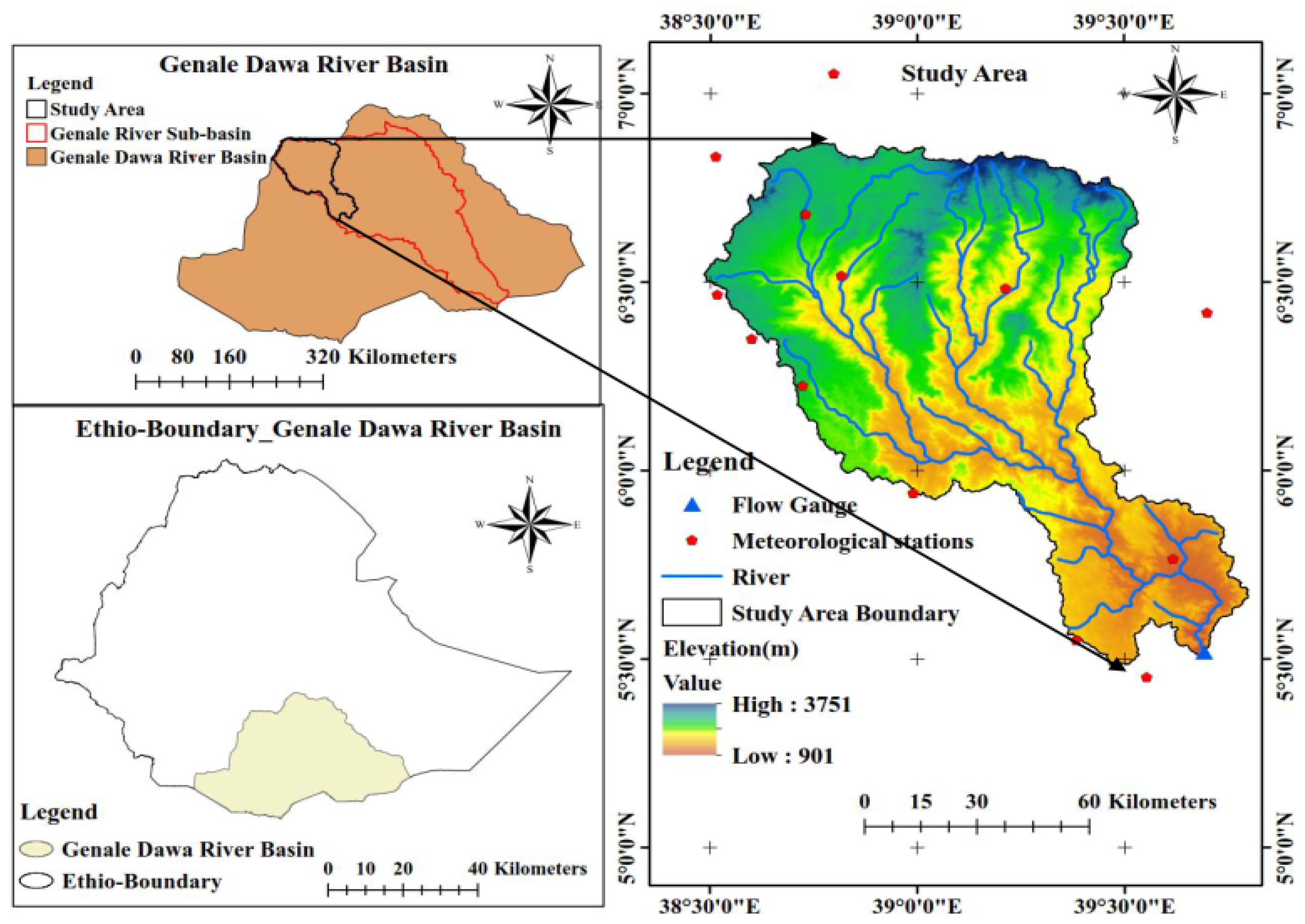
2.1. Description of the Study Area

The Genale River basin is located in the southeastern part of Ethiopia. The basin covers a portion of Southern Nations, Nationalities, and Peoples’ (SNNP), Oromia, and Somali regional states. It is situated between latitudes of 3°30′ and 7°2′ N and longitudes 37°05′ and 43°20′ E. The basin area is about 172,713 km2. It is one of Ethiopia’s three widest river basins [51]. Specifically, the upper Genale River basin (study area) is located between the latitudes of 6°52′ and 5°20′ N and longitudes of 38°30′ and 39°45′ E, and it lies in the upper central area of the basin. It has a basin area of about 10,582.19 km2 (Figure 1). Due to topographic and ITCZ (inter-tropical convergence zone) effects, the basin experiences bimodal type I (three seasons) and bimodal type II (double wet and dry seasons) annual rainfall cycles in the northern (highland) and southeastern (lowland) parts, respectively. The northern and highland area is characterized by three wet seasons, March–May (locally known as belg), June–September (locally known as kiremt), and September–November (locally known as meher) [20]. The lowland and the southeastern parts of the study area experience two wet seasons, one from March to May, with the highest in April, and the other from September to November, with the highest in October [20,52]. The annual average rainfall varies from 1617.7 mm to 591 mm. The annual mean minimum and maximum temperatures range between 6.9 to 16.2 °C and 18.9 to 27.7 °C, respectively. The main river, Genale, emanates in the northwest from the Sidamo Mountains and in the northeast from the Bale Mountains massif [20].

2.2. SWAT Model Input

To evaluate the performance of the SWAT model and to assess the effect of LULC changes on watershed hydrologic characteristics, temporal data such as climate and streamflow data and spatial data such as study area DEM, three different period LULC maps (1986, 2001, and 2016), and a soil map were used.

2.2.1. Study Area DEM (Digital Elevation Model)

A DEM of the upper Genale River basin with a horizontal resolution of 30 m shuttle radar topography mission (SRTM) was obtained from the USGS website. It was used to determine the watershed boundary, sub-watershed, and hydrologic response unit. The DEM was additionally used to identify the subbasin characteristics of the watershed, including elevation, channel slope, slope gradient, reach length, and river network (Figure 1).

2.2.2. Land Use Land Cover Map

LULC is one of the primary factors influencing hydrologic characteristics such as runoff, evapotranspiration, and surface erosion in a watershed, and it is also used in the SWAT model for HRU delineation. To evaluate and understand the hydrological parameters under the effects of LULC changes in the study watershed, the classified LULC maps of 1986, 2001, and 2016 were used separately.

2.2.3. Soil Map

Soil maps of the study basin affecting the hydrological parameters of the basin were used as SWAT model input. The upper Genale River basin soil map was obtained from Food and Agricultural Organization [53] and extracted using ArcGIS10.5 software. From the SWAT database, the soil’s physical and chemical properties, its texture, hydrologic group, bulk density, depth, organic matter content, water capacity, erodibility, and saturated hydraulic conductivities, were extracted. In addition, the required soil physicochemical properties extracted from the SWAT database were compared and verified with the soil survey reports from the Genale Dawa River basin master plan developed by the Federal Democratic Republic of Ethiopia, Ministry of Water Resource [54]. Based on the FAO soil classification system, the study basin contains the soil types of haplic yermosols, eutric nitosols, eutric cambisols, ferric acrisols, and calcaric regosols, which covers about 41.4%, 40.3%, 13.1%, 3.7%, and 1.6%, respectively, of the total watershed.

2.2.4. Meteorological Data

The required daily rainfall and temperature data for 33 years (1984–2016) were used to run the SWAT model. Due to the limitation in the availability of the minimum and maximum temperature data in the study basin, five stations (Arbgona, Bidere, Hager Selam, Haroklo, and Nghele) and rainfall data from ten stations (at Arbegona, Bore, Bidere, Hager Selam, Haroklo, Kibre Mengist, Neghele, Talamokentise, Woreka, and Yirba Muda) were collected from the Ethiopian National Meteorological Service Agency (NMA) Data from three locations (Arbegona, Bidere and Harokelo) were extracted from the Enhancing National Climate Services (ENACTS) dataset. It is a 4 × 4 km resolution dataset reconstructed by integrating data sources from records of local meteorological stations and satellite estimates from NASA (The US National Aeronautics and Space Administration, Washington, WA, USA) and EUMET-SAT (The European Organization for the Exploitation of Meteorological Satellites, Darmstadt, Germany) [55,56]. The performance of ENACTS has been tested at various stations throughout the country and has been proven to perform well [55,56,57].
To make the series for further analyses, the missing values were generated and filled by multiple imputations using fully conditional specification (FCS) implemented by the MICE (multivariate imputation by chained equations) algorithm as described by van Buuren and Groothuis-Oudshoorn [58]. In addition, weather elements such as relative humidity, solar radiation, and wind speed were produced using ARCSWAT, WGNMarker 4. Then, the weather data were arranged in SWAT model format and used for simulation. The first three years of data, from 1984 to 1986, were used as the model initialization phase. The subsequent data, from 1987 to 2016, were used for SWAT analysis.

2.2.5. River Flow Data
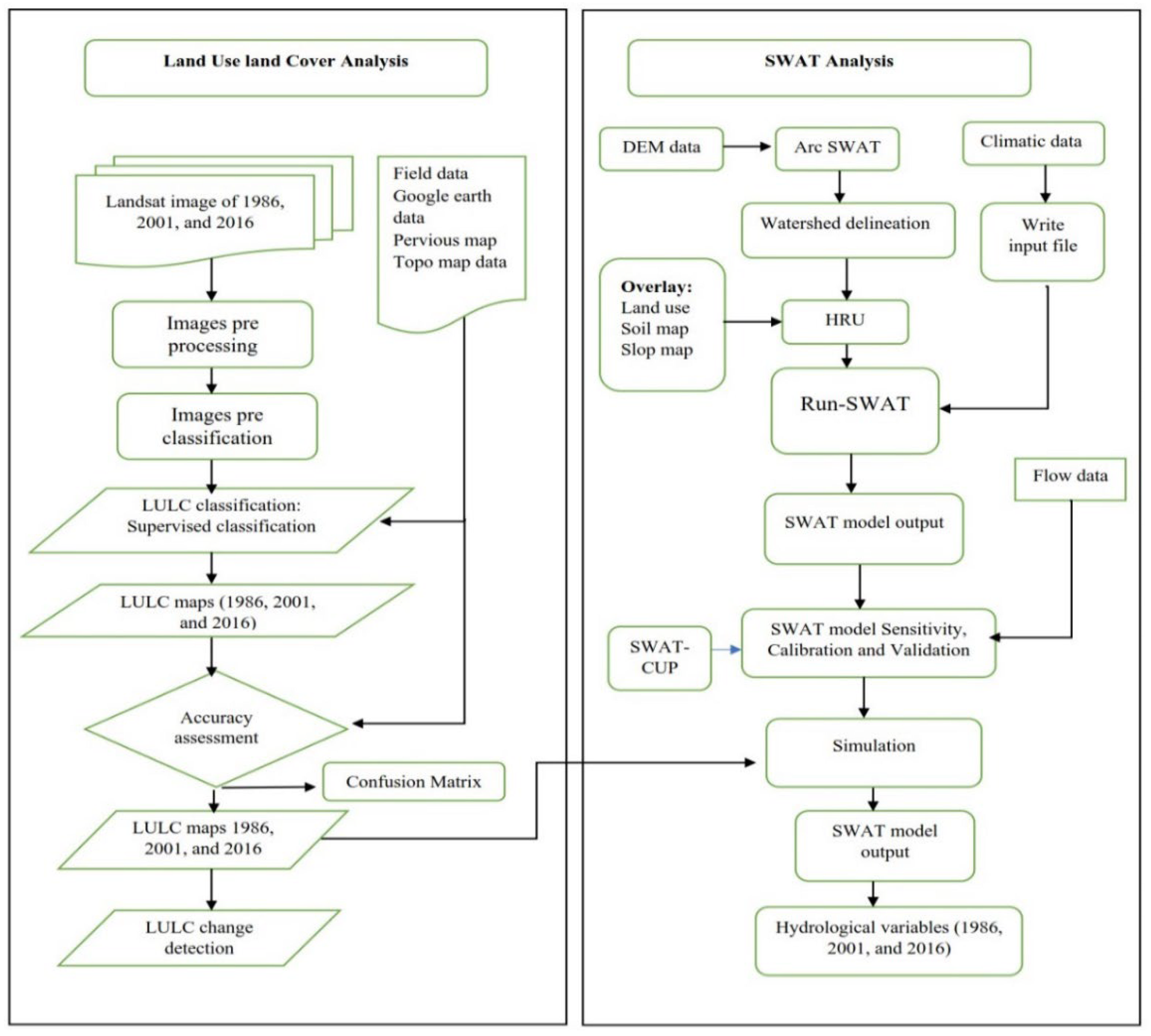
The streamflow data for the period of 1984 to 2011, measured at the Chenemassa hydrological station located at the watershed’s outlet (Figure 1), were obtained from the Ministry of Water, Irrigation, and Energy (MoWIE). The missed values of streamflow data were estimated using multiple imputation. It is the best estimation of missing values [59]. Then the flow data were arranged according to SWAT requirement data format for model calibration and validation. Flow data from 1987 to 2002 were used for model calibration, whereas independent data sets from 2003 to 2011 were used for model validation.

2.3. LULC Analysis

To extract LULC data, cloud-free (<10%) dry season images of Landsat 5 TM (Thematic Mapper) and Landsat 8 OLI (Operational Land Imagery) were used. Landsat images were selected because NASA’s Landsat missions provided free and extensive data on global coverage (since 1972) at a moderate to high level of resolution, and the data have been widely used for detecting LULC changes [60]. The Landsat images at a resolution of 30 m of 1986, 2001, and 2016 were collected from United State Geological Survey (USGS) Earth explorer, available at https://earthexplorer.usgs.gov/ (accesses on 13 November 2020) (Table 1). To cover the entire area of the watershed, three satellites images with path/raw of 167/056, 168/055, and 168/056 were used. The images were selected based on historical drought events and availability of Landsat images. To minimize errors due to different seasonal variation in vegetation distribution or in LULC change detection, images of the same annual season were used [4,61].
Then, the downloaded images were preprocessed in ARC GIS 10.5. For the preprocessing, georeferencing, geometric correction, compositing/layer stacking, mosaicking and clipping were performed prior to image classification [62]. During the preprocessing of satellite images, radiometric and geometric corrections were applied to the raw Landsat images. This approach produces adjusted satellite images that are radiometrically and geometrically corrected. Radiometric corrections are generally used to normalize the multi-temporal satellite images for time-series comparisons. For better interpretation of the scenes, local enhancement (data scaling and histogram equalization) was carried out [62]. Once the preprocessing and mosaicking of the images were completed, the area of interest was clipped using the inbuilt raster processing tools in Arc GIS 10.5.

Image Classification and Accuracy Assessment

In this LULC change analysis, to generate and classify the LULC maps, unsupervised and supervised techniques of classification were employed [44]. The unsupervised method was to generate initial information of the spectral characteristics of clustered pixels prior to the supervised classification [62]. The supervised/maximum likelihood classification was conducted to generate the land cover types using the training sites developed from ground truth data, unsupervised maps, Google Earth, and 1975 topo maps at 1:250,000 scale from EMA (Ethiopian Mapping Agency, Addis Ababa, Ethiopia).
Using the supervised classification maximum likelihood algorithm embedded in ARC GIS 10.5 software, images of the years 1986, 2001 and 2016 were classified based on average total of 360 training points gathered from the digital 1975 topo maps of 1:250,000 scale from EMA, Google Earth, previous LULC maps, and ground-based reference points. To determine the sampling points, systematic purposive sampling was used. For this task, training points from the northern, middle, and southern parts of the study basin were collected. During the field work, at the time of ground truth data collection, in-depth discussions with elders from the area, to recall the past land cover information, were conducted.
In the classification approach, seven major LULC classes such as built-up or settlement, cultivated land, shrubland, forest land, grassland, bare land, and water bodies were identified. Settlement or built-up areas included urban, road network, and rural residential areas such as villages and rural towns; cultivated land meant areas used to cultivate annuals rainfed and irrigated crops; shrubland embraced shrubs, bush, short mixed dense vegetation, and lower-height trees; forestland included areas covered by dense natural forest, trees plantations, and coffee and other dense vegetation; grassland referred to communal and private owned grazing lands and also areas with sparse vegetation dominated with grass; and bare land was areas covered with stones with very little vegetation, exposed rocks and bare soil and degraded areas found in lower rivers and steep mountainsides and water bodies, referred to the main Genale River.
Once the land cover classifications were developed, the LULC maps of 1986, 2001 and 2016 were prepared. Then, by comparing the sample LULC classes of the classified layer and the reference layer, the classification accuracy of the resulting LULC maps was assessed. To evaluate accuracy of 1986, 2001, and 2016 LULC maps, overall, producer’s accuracy, user’s accuracy and Kappa coefficient were computed using Equations (1)–(4), respectively. The details are described by Lillesand et al. [62]:
Overall   accuracy = Total   correctly   classified   pixels Total   of   classified   pixels × 100
Overall accuracy is calculated by dividing the total number of correctly classified pixels (i.e., the sum of the major diagonal) by the total number of reference pixels.
Producer   accuracy = Number   of   correctly   classified   pixels   per   class Number   of   reference   totals   per   class × 100
The producer’s accuracy indicates how well test set pixels of the given cover type are classified.
User   accuracy = Number   of   correctly   classified   pixels   per   class Number   of   classified   totals   per   class × 100
The user’s accuracy is a measure of commission error that indicates the probability that a pixel classified into a given category actually represents that category on the ground.
Kstat = N i = 1 r Xij i = 1 r X RT × X CT N 2 i = 1 r X RT × X CT
where Kstat is Kappa statistic, N is total number of samples, Xij is the product of total number of sample and total diagonal values, XRT is row total, XCT is the column total and r is the number of categories. The statistics or coefficient evaluates the difference between the actual agreement of classified map and chance agreement of random classifier compared with reference data [63]. The overall LULC classification is shown in Figure 2 of the general conceptual framework of the research methodology.
To quantify the percentage share, gains/losses, and percentage change of each LULC classes, the areas of the LULC classes, area comparison analysis of LULCC of two classified LC maps (1986 to 2001, 2001 to 2016, and 1986 to 2016), and percentage of LULC change were computed from the maps. The total gain or loss of LULCC and their percentage between the two periods was computed using Equations (5) and (6) as follows [17,63]:
Gain   / Loss   of   LULCC = final   year   LULC   area     initial   year   LULC   area
LLCC   ( % ) = ( LULC   area   of   the   final   year     LULC   area   of   the   initial   year ) LULC   area   of   the   initial   year × 100

2.4. Description of the SWAT Model Set Up

The Soil and Water Assessment Tool (SWAT) is a semi-distributed and physically based watershed model that runs at a continuous time step [64]. It is developed to test and predict the impacts of change in land use practices and climate on hydrology, agricultural pollutants, sediment movement of large and complex basins [65,66]. The SWAT simulates the hydrologic process of a watershed using two major ways: the land phase and the water or routing phase. The former regulates the amount of water transported, chemicals, nutrients, and sediment loading from the sub-watershed through the channel route, while the latter controls the flow movement up to the basin outlet. Detailed information on the physical processes modeled within SWAT are presented in [67]. To simulate the hydrological processes of the watershed, in the land phase of hydrological cycle, the SWAT used the water balance equation described as follows [67,68]:
SW t = SW o   + i = 1 t P day     R surf     E a     Q gw     Q vad
From Equation (7), SW0 and SWt represent the initial and final soil water content on day i (mm); Pday, Rsurf, Ea, Qgw, and Qvad represent the amount of precipitation, surface runoff, evapotranspiration, return flow, and water entering the vadose zone from the soil profile, respectively, on day i (mm), and t is the time (days).
The SWAT model calculates surface runoff from the watershed using either the USDA Conservation Service Curve Number (SCN-CN) or the Green and Amp method [67]. For this study, to compute surface runoff for each HRU, the SCN-CN method was used (Equation (8)) [69]:
Rsurf = Pday 0.2 S 2 Pday + 0.8 S
where Rsurf is depth of daily accumulated runoff (mm), S is a retention parameter, and Pday is the daily rainfall depth (mm). The above equation indicates that surface runoff in a watershed occurs when the depth of rainfall in a day (Pday) is greater than 0.2S.
In terms of curve number (CN), parameter S is computed by Equation (9). S is affected by slope, types of soil, and land use management practices:
S 2.54 = 1000 CN 10  
According to Arnold et al. [64], CN is a significant parameter that determines the surface runoff of the catchment during the model calibration.
SWAT model has three options to compute evaporation, Hargreaves, Priestly–Taylor, and Penman–Monteith formulas as cited by Neitsch et al. [67]. The Hargreaves method, due to its simplicity and data availability, was used for calculating evapotranspiration.

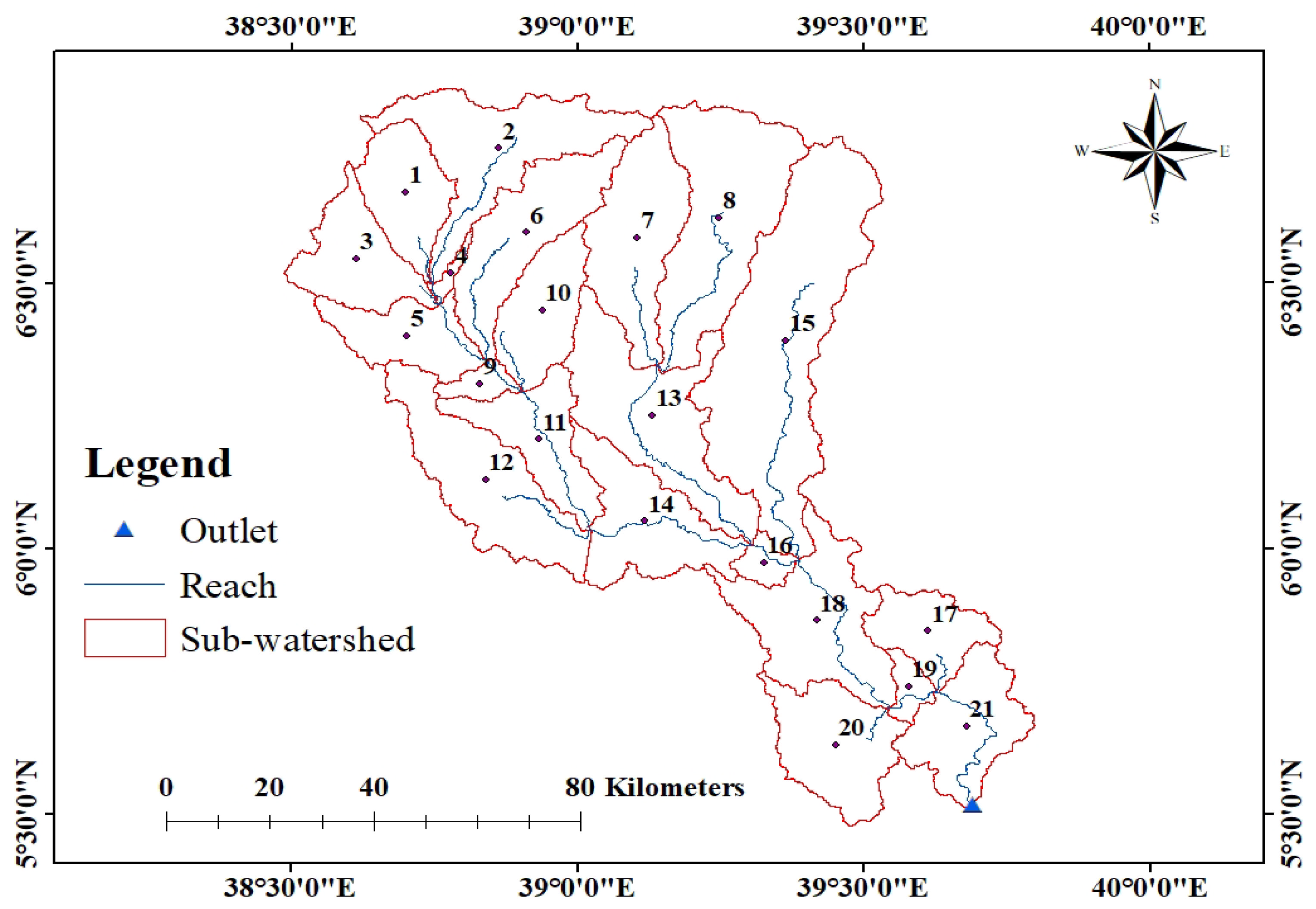
2.5. Watershed Delineation

To delineate the study basin, the SWAT model was set up using the ARCSWAT install of the ARCGIS extension. Using the study area DEM and watershed outlet location point (at Chenemassa gauging station), the watershed, sub-watershed, and reaches of the watershed of the upper Genale basin were delineated. With this delineation process, 21 sub-watersheds were defined (Figure 3).
Then, after watershed and its parameters had been determined, based on a combination of land cover map, soil map, and slope categories with a 10% threshold, 352, 337, and 350 HRUs for the 1986, 2001 and 2016 LULC models, respectively, were created.

2.6. Model Simulation and Sensitivity Analysis

The study area watershed hydrological processes were simulated using hydro-climatic data. The climate data from 1984 to 2016 were arranged according to the SWAT requirement format. Data from 1984 to 1986 were used to initialize the model, and the subsequent data from 1987 to 2016 were used for parameter sensitivity analysis and model calibration.
The SWAT model has a large number of hydrological parameters that affect stream flow, and calibrating them all is difficult and time-consuming. Therefore, identifying the more sensitive parameters that affect model output is valuable [36]. The parameter sensitivity analysis helps to detect the most influential flow parameters that are used for calibration and validation in the model [70]. To differentiate the most influential SWAT flow parameters in this study, twenty-one flow parameters from SWAT-CUP and literature were carefully chosen at the initial phase. Then, using multiple regression methods with Latin hypercube parameters of the objective function, t-stat and p-values, sensitivity of the parameters were determined. The t-stat and p-values indicate the degree and level of sensitivity to flow parameters, and small absolute t-stat values indicate less sensitivity, while large values indicate higher sensitivity. Smaller p-values indicate greater sensitivity, while larger values indicate less sensitivity [68,71].

2.7. SWAT Model Calibration and Validation

For model calibration and validation, recorded daily river flow data at the Chenemasa hydrological station were used. The daily flow data were changed to monthly flow data and arranged according to the SWAT data format requirement for model calibration and validation. Model calibration was then executed using the monthly flow data series ranging from 1987 to 2002. Following the identification of calibrated flow parameters, validation was carried out using flow data ranging from 2003 to 2011. To execute calibration and validation processes, SUFI-2 (sequential uncertainty fitting) algorithm in SWAT-CUP2012 version 5.1.6 were used [71]. SUFI-2 is a popular and extensively used program for model uncertainty, calibration, and validation analysis in different parts of Ethiopia [2,4,26,28,31,36,43,44,72,73].

2.8. Model Performance Evaluation

The SWAT model’s performance was evaluated by comparing the fitness of the output of the measured stream flow data with that of simulated model output. The statistical indices assess the closeness between the measured streamflow data and the corresponding simulated output. Hence, for this study, PBIAS (percent of bias), R2 (coefficient of determination), and NES (Nash–Sutcliffe efficiency) were used to evaluate the performance of the model. These statistical parameters are the most widely used for model performance evaluation [21,74]. The performance indices of R2, NSE, and PBIAS were calculated using Equations (10)–(12), respectively.
The regression coefficient (R2) describes the degree of collinearity between the measured streamflow data and simulated output data [75]. R2 varies from 0 to 1. The closer R2 is to 1, the less the error variance, i.e., the agreement between the observed flow data and the simulated output is higher. Equation (10) is used to compute R2:
R 2 = i = 1 N Oi O ¯ Pi P ¯ i = 1 N Oi O ¯ 2 0.5 i = 1 N P Pi ¯ 2 0.5 2
The Nash–Sutcliffe efficiency (NSE) is a statistical index that is used to assess how much the model accurately simulated or to determine how the measured data and the simulated output closely fits in 1:1 line [75,76] and calculated as described in Equation (11):
NSE = 1 i = 1 N Oi Pi 2 i = 1 N Oi O ¯ 2
The percent of bias (PBIAS) as explained by Moriasi et al. [75] was employed to determine how much the simulated output will be smaller or larger than the measured counterparts. According to [75], the PBIAS was computed using Equation (12):
PBIAS = i = 1 N oi pi i = 1 N oi × 100
where Oi and Pi are the measured and simulated flow, respectively, and O ¯ and P ¯ are the average measured and simulated flow, respectively.
According to Moriasi et al. [75], the performance of the model is acceptable when R2 and NSE are greater than 0.6 and 0.5, respectively, and PBIAS is in the range of ± 25%. R2 varies from 0 and 1, where R2 approaches 1 indicates less error. The NSE ranges from −∞ to 1. If NSE is closer to one, the model performance is best. On the other hand, the closer the PBIAS to 0 indicates best simulation. Positive values show that the model underestimates the simulation, whereas a negative value shows the model overestimates the simulation [77].

2.9. Impacts of LULC Change on Hydrological Processes

Understanding the hydrologic response of a watershed due to changes in land cover characteristics is imperative for managing water resource measures [44]. To evaluate the hydrological process under the impacts of land cover modifications, the SWAT model was executed for the 1986 LULC, 2001LULC, and 2016LULC scenarios using the same climatic data from 1987–2016. The study was carried out with the “fixing-changing” technique. The method works by changing the land cover input data while fixing the other data in the SWAT model, such as climate, soil, and DEM data. This approach has been used by various scholars across the world [22,37,44,78]. The effect of the LULC change on the basin’s hydrologic characteristics and water resources was calculated by comparing SWAT outputs for LULC maps of (1986, 2001, and 2016). The differences in observed outputs represented the impacts of LULC change on hydrologic response and water resources in the catchment.

3. Results and Discussions

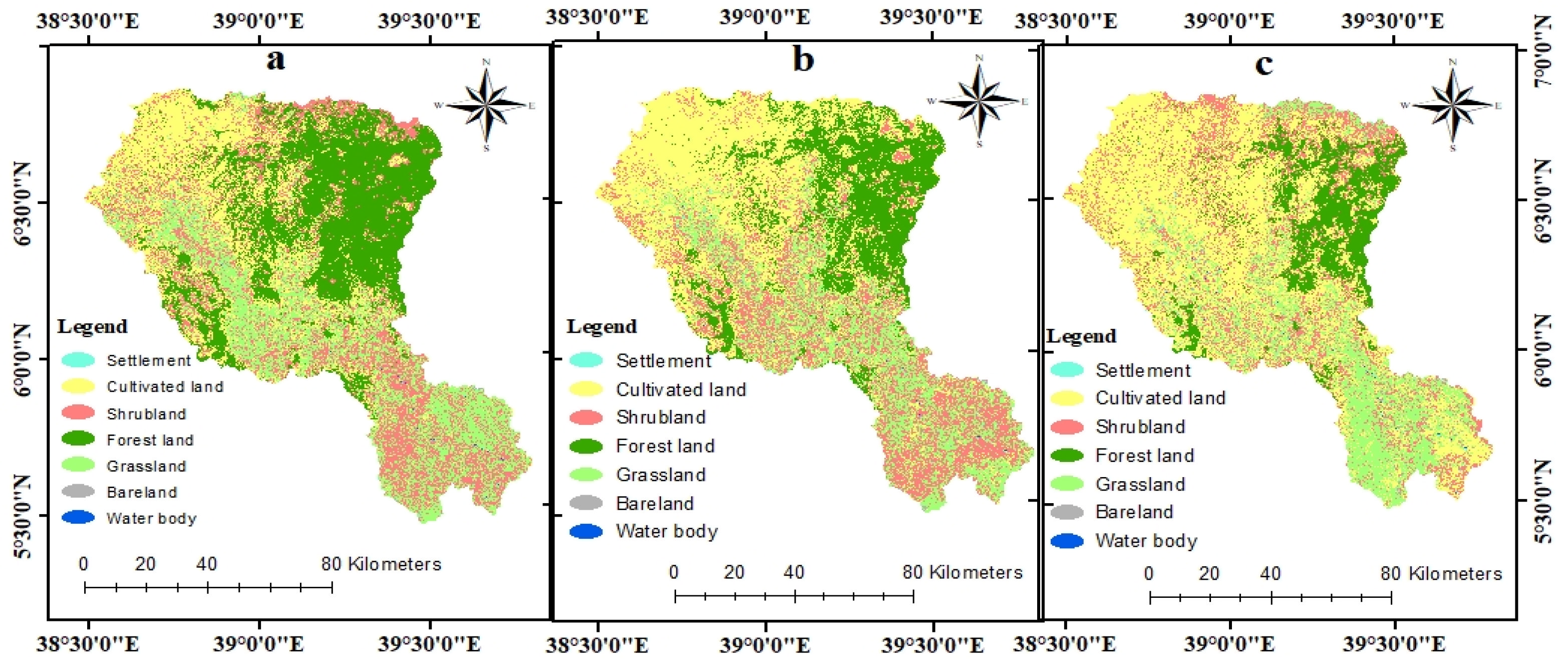
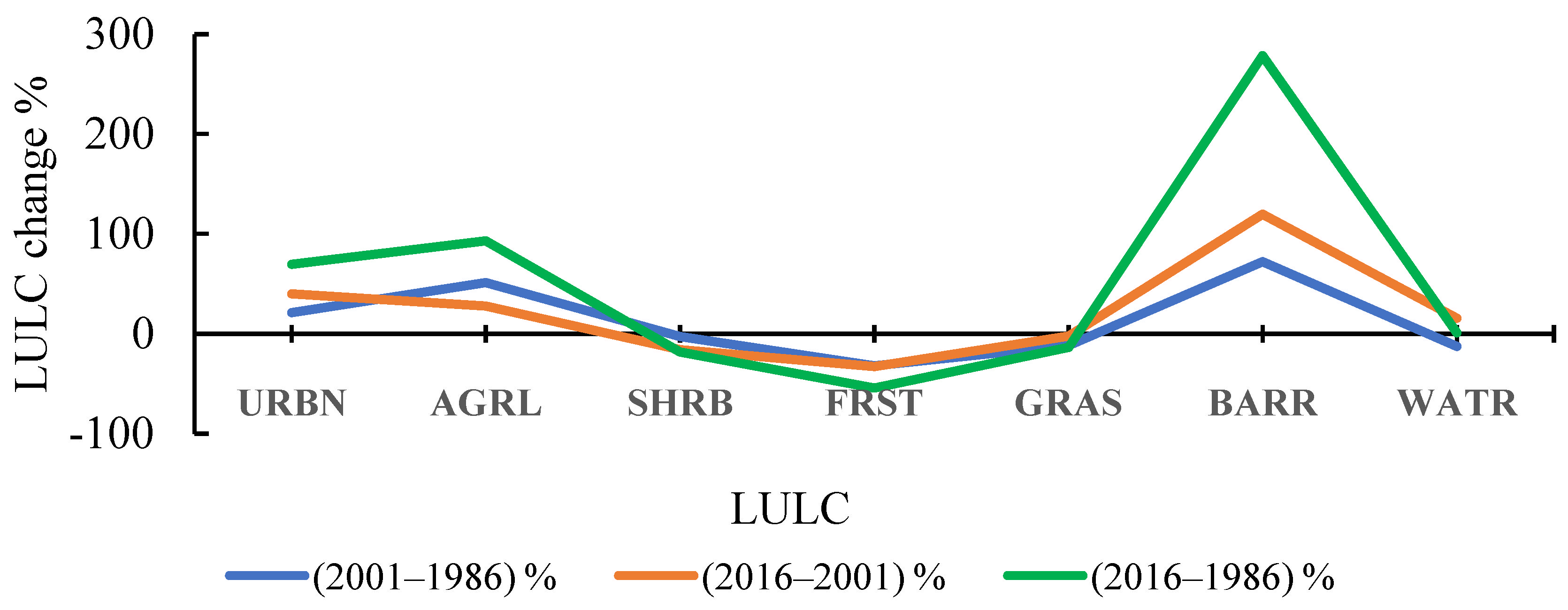
3.1. Land Use/Land Cover Change Dynamics

Based on spectral characteristics and Landsat image processing, seven land cover types were developed. The areal coverage and the spatial distribution of the 1986, 2001, and 2016 LULC classifications are depicted in Table 2 and Figure 4, respectively. The expansion of cultivated land and a significant reduction in forest land occurred in the highland area of the catchment. In addition, significant portions of grassland and bushland were found in the lower part of the catchment. Furthermore, the analysis in Table 2 and Figure 4 showed that in 1986, about 29.6% of the land was covered with forest, followed by cultivated land, shrubland, and grassland, which covered about 24.4%, 23.85%, and 21.8% of the total area, respectively. On the other hand, settlement, bare land, and water bodies covered about 0.16%, 0.16%, and 0.06% of the total area, respectively. However, in 2001, cultivated land, settlement, and bare land coverage increased to 36.85%, 0.2%, and 0.3%, while forest, shrubland, and grassland decreased to 20.1%, 23.2%, and 19.3%, respectively. In 2016, settlement, cultivated land, and bare land further increased to 0.28%, 47.08%, and 0.62% while forest, shrubland, and grassland decreased to 13.53 %, 19.5%, and 18.9%, respectively (Table 2).
During the last three decades, between 1986 and 2016, the upper Genale River basin experienced a substantial alteration in major LULC. Cultivated land, settlement, and bare land had all been increasing in a continuous manner. In contrast, forest, shrubland, and grassland coverage decreased, possibly as a result of growth in population and increased demand for agricultural production. The finding of this study agrees with the studies by [15,79] in the Genale Dawa basin.
The LULC investigation revealed that the rate and pattern of change varied significantly across land uses and study time periods. Between 1986 and 2001, cultivated land increased by 51.3%, and between 2001 and 2016, it increased by 27.7%. Between 1986 and 2001, and 2001 and 2016, about 132,244.4 ha and 108,181.4 ha of land cover were converted into agricultural land, with annual average rates of 8816.3 ha and 7212.1 ha, respectively. However, between 1986 and 2001, the coverage of forest, grass, and shrublands was reduced by 32%, 11.45%, and 2.85%, respectively. Between 2001 and 2016, forest, grass, and shrublands further decreased by 32.7%, 2.2%, and 15.7%, with rates of 4645.6 ha, 302.7 ha, and 2565.5 ha per year, respectively. Between 1986 and 2001 and 2001 and 2016 study periods, bare land expanded rapidly at a rate of 72.3% and 119.8%, respectively. Throughout the study period (1986–2016), the area of cultivated land, settlement area, and barren land increased by 93.3%, 69.7%, and 278.6%, respectively. Through these same periods, the coverage of forestland, shrubland, and grassland reduced by 54.3%, 18.1%, and 13.4%, respectively (Table 3 and Figure 5).
Table 4, Table 5 and Table 6 show the detection of LULC modification and the transitional matrix for each LULC. The totals in the column (Table 4) correspond to land cover values in 1986, while the totals in the row relate to land cover classifications in 2001. The proportion of the corresponding land cover that remained under its original cover is represented by the diagonals of the change matrix.
From 1986 to 2001, about 57.2% of the total LULC remained unchanged in 2001, and about 42.8% of the total LULC areas were converted to other types. The transition matrix analysis also revealed that in 2001, approximately 83.6%, 68.5%, 52.3%, 58.8%, 47.4%, 54.1%, and 87.5% of settlement, cultivated land, shrubland, forestland, grassland, bare land, and water bodies remained unchanged. As can be inferred from Table 4, about 36.5% of grassland, 19% of shrub, 25.8% of forest, and 26.3% of bare land were converted into cultivated land between 1986 and 2001. Babiso et al. [80], working in the Wallecha watershed in southern Ethiopia, indicated that the transformation of forestland, grassland, and shrubland into agricultural land is primarily related to the need for more cropland to fulfill the food demands of an expanding population and the loss of soil productivity due to unsustainable crop farming techniques
According to the change matrix between 2001 and 2016, about 57.54% of total land cover remained under its original cover in 2016 (Table 5). In addition, in 2016, approximately 97.4% of settlements, 78.1% of cultivated land, 33.3% of shrubland, 49.7% of forestland, 55.7% of grassland, 61.7% of bare land, and 100% of water bodies remained unchanged. Furthermore, Table 5 also showed that cultivated land expanded significantly, primarily at the cost of shrubland (35.2%), grassland (29%), and forest land (22.3%).
During the last 30 years (1986–2016), the magnitude and direction of LULC transformation varied continuously and substantially in the study basin. From 1986 to 2016, about 43.7% (462,441.8 ha) of the total land cover remained the same as it was in 1986, while the remaining 56.3% (595,777.4 ha) shifted to another land cover class (Table 6). Cultivated land expanded significantly at a rate of 8014.2 ha per year during this time period. From the totals covered in 1986, approximately 37.2% (933,89.33 ha) of shrubland, 43.2% (998,56.25 ha) of grassland, and 36.5% (114,225.2 ha) of forest land were shifted to cropland. As a result, it is clear that the most dynamic land cover classes were forest, shrubs, and grass land, which were mostly converted to cultivated land. In the same way, settlement and bare land coverage also expanded during the study period. Each of these land cover types is heavily influenced by land form, soils, and climate properties as in the rest of Ethiopia. Natural vegetation cover, particularly forest land, is being heavily encroached by cultivated lands as a result of high population growth, followed by people’s and the government’s preferences for food and export crops in order to alleviate the prevailing food and employment insecurity [81]. Various studies in Ethiopia revealed that settlement areas and cultivated lands were replacing forest, shrub, and grass lands [8,82,83,84]. Similarly, LULC changes were also reported by different scholars in different parts of the Genale Dawa basin [15,79,85,86] For instance, Hailemariam et al. [85] reported a total loss of 123,751 ha of forests and an expansion of cultivated land by 292,294 ha in 30 years in the Bale mountains eco-region. The increasing demand for land for building and cultivation, the demand for fuel wood and fodder, institutional and policy changes regarding land resource management, and an absence of adequate technology to enhance farming practices for socioeconomic purposes and income generation all contributed to land use conversion, primarily the destruction of natural vegetation [4,82]. According to Hailu et al. [6] and Betru et al. [3], the main reasons for land cover changes are the conversion of forestland, shrubland, grassland into settlement, cultivated, and bare land are poverty, population growth, unemployment, lack of off-farm employment, institutional and policy changes, low level of awareness of natural resource conservation and management, and a lack of the proper execution of legal and institutional frameworks related to natural resources managements The Genale Dawa master plan report [81] showed that LULC changes in the basin mainly influenced with fast growth rate of population, occurrence of recurrent drought, shortage of cultivated land, illegal utilization forest resources, and the inclination of the government to implement different land and water resource development activities

3.2. Accuracy Assessment of LULC Images

The accuracy of the 1986, 2001, and 2016 classified images assessed by calculating the kappa coefficients and the user’s, producer’s, and overall accuracy. Table 7 displays the summarized LULC classification accuracy for 1986, 2001, and 2016. Based on the error matrix, the overall accuracies of the classified images of the 1986, 2001, and 2016 were 85.3%, 87%, and 90.05%, respectively. The overall accuracy of the classified images exceeded the minimum recommended accuracy of 85% [87]; about 85%, 87%, and 90% of the LULC classes were precisely classified. For 1986, 2001, and 2016, the kappa statistics were 82.5%, 84.7%, and 88.3%, respectively, indicating that the agreement between the identified LULC classes and the geographical data is strong. According to Viera and Garrett [88], kappa higher than 0.8 represents strong agreement, whereas values ranging from 0.61 to 0.8 indicate very good agreement. The user accuracy of individual classes for 1986, 2001, and 2016 ranged from 77.6% for cultivated land and 100% for water bodies. In these same years, the producer accuracy ranged from 77.6% for grass land and 100% for forest land and water body.

3.3. Sensitivity Analysis

For model calibration and validation, the key parameters that affect the streamflow in the SWAT model were identified using sensitivity analysis [64]. Throughout the simulation period, the SWAT-CUP software SUFI-2 algorithms were used to determine the most significant flow parameters. The sensitivity of the stream flow was calculated using average monthly streamflow data for 25 years (1987–2011) recorded at the Chenemassa hydrological station. During the initial phase of the process, twenty-one flow parameters were carefully selected from the SWAT-CUP and the literature. Out of these initially selected parameters, 10 sensitive flow parameters were identified based on the t-stat (ranging from 7.86 to 0.65) and the p-value (ranging from 0 to 0.5) (Table 8).
Among the identified parameters, the ALPHA_BF.gw, the runoff SCS curve number, CN2.mgt and CANMX.hru were found to be the three most sensitive parameters with respect to streamflow. CN2, mgt is the most influential flow parameter in most Ethiopian watersheds [31].

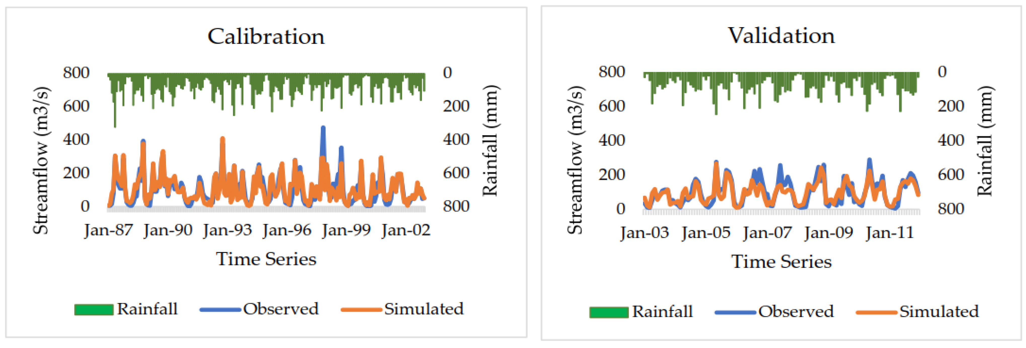
3.4. Model Calibration and Validation

The SWAT model was calibrated and validated using the identified key sensitive flow parameters (shown in Table 8) on the measured streamflow data at Chenemassa station. During the process, the monthly streamflow data from 1987 to 2002 and from 2003 to 2011 were used for model calibration and validation, respectively. To improve the performance of the model during calibration, the selected parameters were changed iteratively within a realistic range until reasonable agreement between observed and simulated streamflow output was obtained (Table 9). Then, after obtaining a reasonable result, the validation was performed using the same set of calibrated flow parameters. During the processes, multiple calibration runs were carried out, and finally, the calibration range and their corresponding best fitted values were obtained and are presented in Table 9.

3.5. Performance Evaluation

The statistical indices of the model calibration and validation results are summarized and presented in Table 10. In this table, two indices, the P-factor and the R-factor, are expressed. Together they show the model calibration’s strength as well as the uncertainty assessment of the simulation results [72]. The percentage of observation bracketed by the 95% prediction uncertainty (95PPU) was 88% for the calibration period and 81% for validation. The R-factor is a measure of the width of the 95PPU band that is determined by dividing the 95PPU average thickness by the standard deviation [70]. The calculated R-factors were 1.02 and 0.87 during the calibration and the validation periods, respectively. According to Abbaspour [71], the closeness of the P-factor and the R-factor is used to assess the goodness of calibration and prediction uncertainty. The P-factor should ideally be 1, representing 100% bracketing of the measured data, hence capturing or accounting for all the correct processes, while R-factor should ideally be close to 0 to match the measured data [71].
Furthermore, Table 10 shows additional information on the statistical valuation results of the model calibration and validation periods for mean monthly flow. The result demonstrated that R2, NSE, and PBIAS of the SWAT model performed well. That is, the SWAT model result showed a good match between observed and simulated monthly flow with NSEs of 0.73 and 0.72 for the model calibration and validation periods, respectively. The R2 result also showed that the model had good agreement between observed and simulated streamflow, with values of 0.78 and 0.74 during the calibration and validation periods, respectively.
The PBIAS for the model was −3.2% for the calibration period and 3.9% for the validation period. The result indicated that the flow during calibration with reference to the observed flow was slightly overestimated. On the other hand, during the validation period, PBIAS indicated that the SWAT model underestimated the simulated flow.
The simulated and observed streamflow hydrographs of the calibrated model displayed that the SWAT model underestimated the peak streamflow of August 1993 and 1996; November 1997; and July, September, and October 1998 in the calibration period, while in the validation period, the model underestimated most of the simulated streamflow (Figure 6).
Figure 7 depicts the scattered plot of the linear regression of the measured and simulated flow of model calibration and validation. The coefficients of determination (R2) for the calibration and validation periods were 0.78 and 0.74, respectively. This indicates a good relationship between the observed and simulated streamflow graphs (Figure 6).
Overall, based on the statistical metrics of R2, NSE, and PBIAS, the SWAT model findings indicated that the measured and simulated monthly streamflow were in good agreement in the study area river basin. Previous research conducted in the Genale Dawa and the surrounding river basin showed that the calibrated and validated SWAT model R2 and NSE ranged from 0.6 to 0.90 and from 0.55 to 0.90, respectively [89,90,91,92]. For instance, research conducted by Negeo and Sarma [90] in the Genale Dawa basin showed that during calibration and validation, NSE was 0.81 and 0.78, and R2 was 0.87 and 0.85, respectively. As a result, the SWAT model is appropriate for further application in understanding the hydrological component and quantifying the potential impacts of LULC change on water resource in the study watershed.

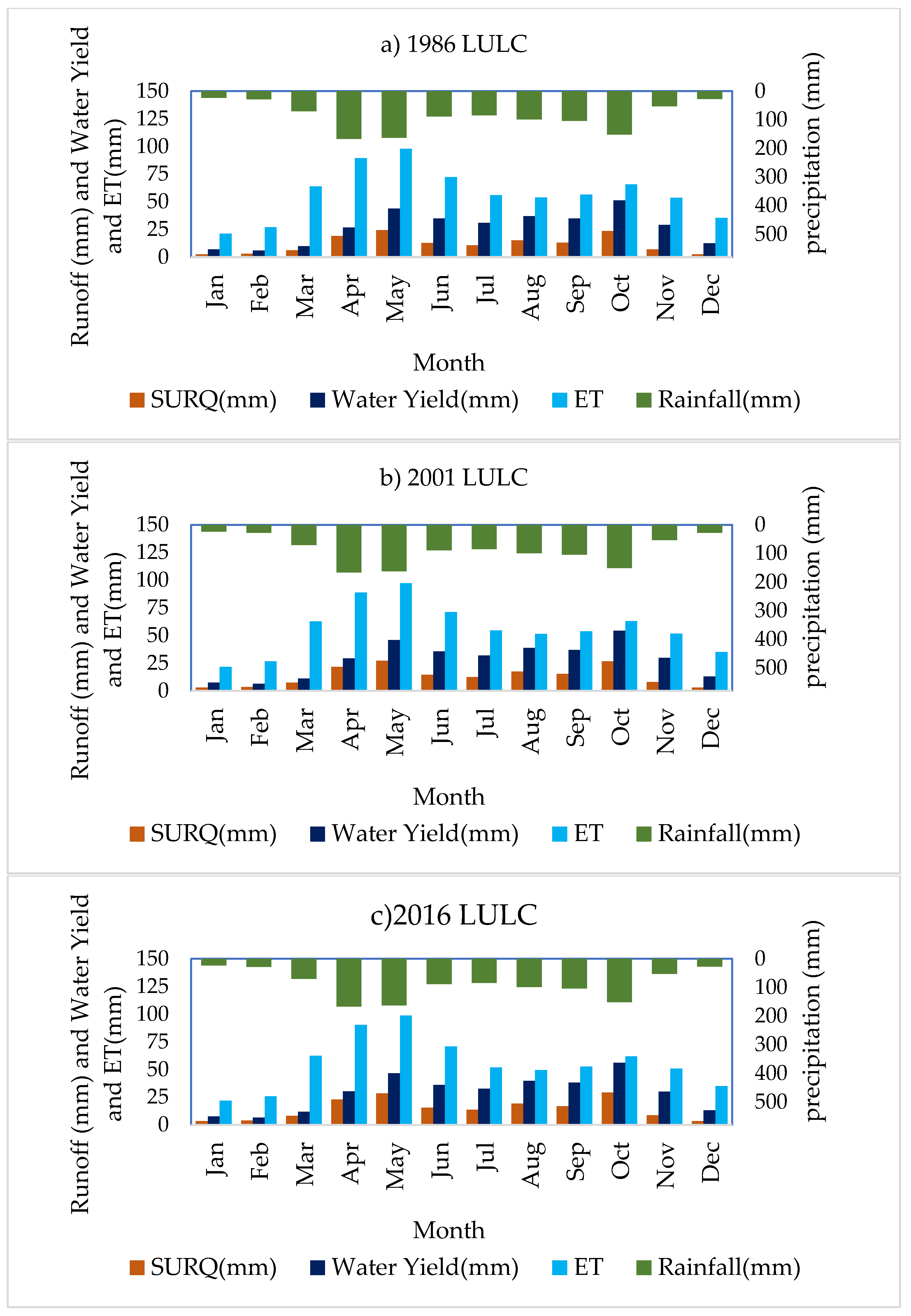
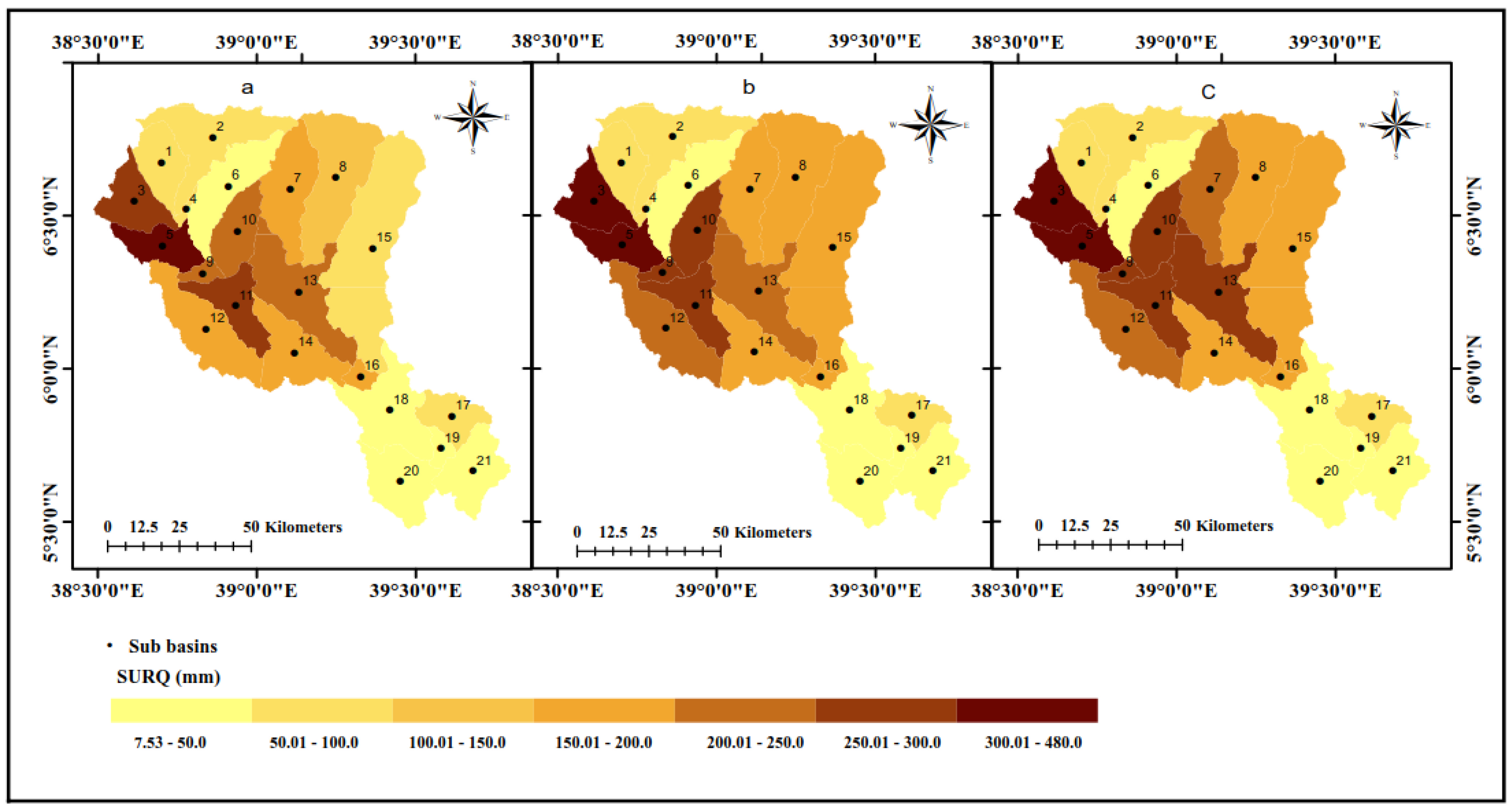
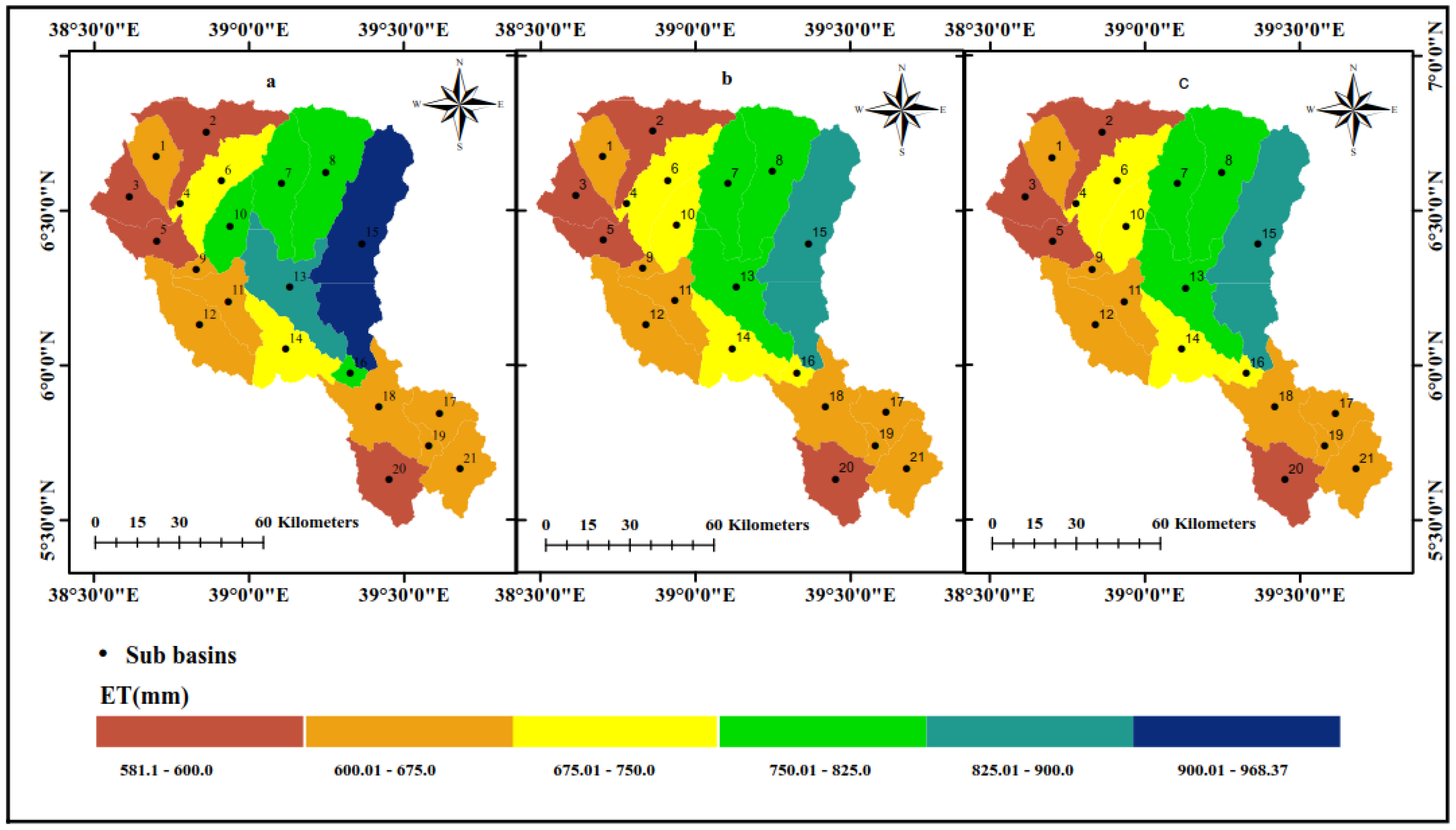
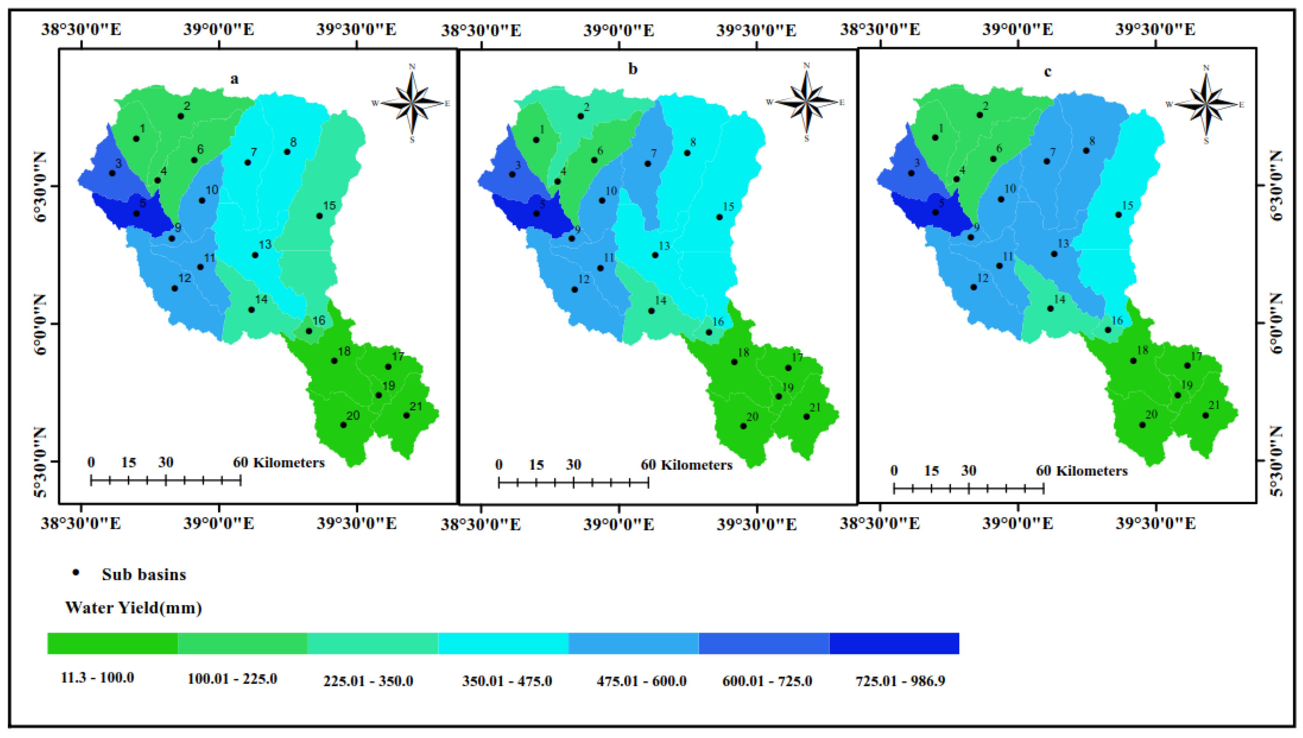
3.6. Effect of Land Use Land Cover Change on Hydrological Process

Based on the simulated precipitation, runoff, evapotranspiration, lateral flow, groundwater flow, and water yield of the SWAT models, the hydrological responses to the 1986, 2001, and 2016 LULC models were examined and are presented in Table 11.
The results during the 1986 to 2001 period showed the annual average runoff in the watershed increased from 139.87 mm to 159.03 mm, and in 2016, it further increased to 171.57 mm, which indicated that there was a 13.7% and 7.9% increment of surface runoff between 1986 to 2001 and 2001 to 2016. The model output also showed that between 1986 and 2016, surface runoff increased by about 31.7 mm, which shows 22.7% increment. Similarly, during the 1986 to 2001 period, the annual total water yield in the study basin was raised from 324.42 mm to 339.63 mm, and to 347.32 mm in 2016. Evidently, this is related to the expansion of settlement, agriculture, and bare land area and the diminishing of forestland, bushland, and grassland throughout the study period, which has a direct influence on total water yield and runoff. In comparison with degraded land and cultivated land, the presence of vegetation on a given landscape increases infiltration depth and initial abstraction, and this allows for more recharge in a given watershed [15].
A number of studies in various parts of Ethiopia have witnessed the same results as this one [15,44,79,89,93]. For example, Aredo et al. [15], in the Genale Dawa River basin in the Shaye Catchment, showed that the increase in cultivated land and built-up areas, as well as a continuous depletion of natural vegetations, contributed to the production of higher runoff in the watershed. Similarly, another study by Messele and Moti [79], in the Weib catchement in the Genale Dawa River basin, concluded that the rapid alteration of vegetation cover such as grass, shrubs, and forestland to agricultural and settlement areas had resulted in more runoff. Another study in the Lake Ziway watershed by Abraham and Nadew [72] showed that the change in land cover from 1996 to 2014 increased annual runoff from 67.5 mm to 129.1 mm and from 40.6 mm to 59.6 mm in the Katar and Meki river basins, respectively. The finding indicated that the land use alterations are the primary causes of increased surface runoff in both watersheds.
Furthermore, the analysis result showed that in the 1986, 2001 and 2016 LULC models, 13.2%, 14.99%, and 16.2% of the basin precipitation converted to surface runoff, while 692.49 mm, 676.76 mm, and 670.34 mm of the precipitation was lost by ET, which is about 65.3%, 63.8%, and 63.2% of precipitation, respectively. These results indicated that the reduction in ET in the watershed was related to the reduction in forest coverage. Moreover, groundwater and lateral flow declined from 145.46 and 38.68 mm in 1986 to 141.31 and 37.92 mm in 2001, and then to 138.34 and 36.08 mm in 2016. On the other hand, compared with the earlier historical LULC data of 1986 and 2001, the recent land cover of 2016 yields higher runoff and water yield and lower groundwater and lateral flow. During the entire period (1986 to 2016), groundwater flow reduced from 145.46 mm to 138.34 mm.
In general, the occurrence of LULC change over the last 30 years (1986–2016) resulted in increased mean annual runoff and total water yield, as well as a reduction in groundwater flow, lateral flow, and evapotranspiration in the watershed. However, the rates of increase and decrease in hydrological components were associated with the rate of LULC changes. For instance, the rates of vegetation reduction (forest, shrub, and grassland) and agricultural expansion during 1986–2001 were higher than in 2001–2016. Consequently, the rate of increase in surface runoff and total water yield was higher during the 1986–2001 period compared with the 2001–2016 period. The reduction in groundwater recharge and the increase in surface runoff are linked with the expansion of agricultural land as well as a significant reduction in vegetation cover. The reduction in forest cover reduced the soil infiltration capacity, which resulted in a large portion of rainfall being converted to runoff, which caused a decline in groundwater and lateral flow. Furthermore, the reduction in evapotranspiration is related to the decline in forest cover and a shortage of soil moisture [26].
The monthly distribution of simulated precipitation, runoff, evapotranspiration, and water yield in Figure 8 shows that the highest values of monthly average surface runoff, evapotranspiration, and water yield were noted during the two main rainy seasons, which run during March, April, and May and September, October, and November. The larger values of runoff, evapotranspiration, and water yield found during these seasons were associated with the substantial amounts and rainfall patterns during the rainy season. Bekele et al. [73] confirmed that the amount and pattern of rainfall are the most influential aspects in the hydrologic process.
The spatial distribution of the water-balance components for the 1986, 2001, and 2016 LULC models at subbasin scale are presented in Figure 9, Figure 10 and Figure 11 and Table S1. The illustrations help in understanding the hydrologic components of the watershed. At the subbasin scale, in the 1986, 2001, and 2016 LULC models, the annual average runoff in the upper Genale River basin varied from 7.75 mm to 427.51 mm, 7.53 mm to 443.09 mm, and 9.72 mm to 476.65 mm, respectively (Figure 9). The figure also depicts that subbasin 20 contributed the least amount of runoff, whereas sub basin 5 produced the most. In the 1986, 2001, and 2016 LULC models, annual mean surface runoff increased in the majority of the subbasins. The observed land cover change over the past 30 years has resulted in changes in runoff and other hydrological components.
The annual evapotranspiration in the subbasin varied from 581.06 mm to 968.37 mm, 563.61 mm to 895 mm, and 582.21 mm to 856.14 mm in the 1986 LULC, 2001 LULC, and 2016 LULC models (Figure 10). The figure also depicts that subbasin 15 contributed the most evapotranspiration; this is due to the fact that subbasin 15 was covered with a significant amount of vegetation. Nicholls et al. [94] confirmed that the rate of evapotranspiration was higher in areas covered with forest than in other land covers. Furthermore, the annual average water yield at the subbasin level varied from 11.35 mm to 985.77 mm, 11.3 mm to 986.89 mm, and 13.93 mm to 983.99 mm in the 1986, 2001, and 2016 LULC models, respectively (Figure 11).
Overall, the reduction in vegetation cover in the landscape, as well as increases in cultivated land, settlement area, and barren land, have had a substantial impact on the hydrologic processes in the study basin. Negese [16] indicated that in Ethiopia during the last forty years, due to the alteration of natural vegetation (grassland, forestland, and shrubland) into built-up area and agricultural land, the mean annual stream flow, surface runoff, sediment yield, soil erosion rate had increased. On the contrary, the observed changes have decreased the groundwater recharge, groundwater flow, and evapotranspiration.

4. Conclusions

A physically continuous, semi-distributed SWAT model was used to understand the hydrological processes of the upper Genale River basin over three different LULC periods (1986, 2001, and 2016). The SUFI-2 algorithm in the SWAT-CUP2012 software was executed for model calibration, validation, and sensitivity analysis. The performance of the model calibration and validation were evaluated using R2, NSE, and PBIAS statistical parameters and monthly measured stream flow data. Flow data from 1987 to 2002 and 2003 to 2011 were used for calibration and validation, respectively.
During the sensitivity analysis, it was discovered that the groundwater and hydrologic response parameters were more sensitive to streamflow than other parameters. During the calibration period, R2, NSE, and PBIAS were 0.78, 0.73, and −3.2%, respectively, while during the validation period, R2, NSE, and PBIAS were 0.74, 0.72, and 3.9%, respectively. The performance of the model calibration and validation showed that the evaluation results were acceptable. That is, the SWAT model performed well and is applicable to simulating hydrological processes in the study basin.
The image analyses during 1986, 2001, and 2016 in the upper Genale River basin showed that the extent of settlement, cultivated land, and barren land area significantly increased by 93.3%, 69.7%, and 278.6%, respectively. On the contrary, forestland, shrubland, and grassland diminished by 54.3%, 18.1%, and 13.4%, respectively. These continuous and dynamic modifications of LULC had a substantial effect on the watershed hydrology of the study area. The expansion of settlement, cultivated, and bare land and the reduction of vegetation cover (grassland, shrubland, and forestland) during the 1986 to 2016 period caused an increase in the annual runoff and water yield. On the other hand, the observed land cover changes decreased groundwater and lateral flow. The hydrological responses of LULC for the 1986, 2001, and 2016 models showed that the average annual runoff increased by 13.7% and 7.9% between 1981 to 2001 and 2001 to 2016. Similarly, between 1986 to 2001 and 2001 to 2016, the annual total water yields increased by 4.69% and 2.26% in the study watershed, respectively. The model output also exhibited that between 1986 and 2016, surface runoff increased by about 31.7 mm, which is a 22.7% increment. Moreover, in the 1986, 2001, and 2016 LULC models, about 43.2%, 47.01%, and 49.6% of runoff contributed to the total flow. The model also showed that groundwater and lateral flow contributions were reduced through the entire study period. Evidently, this result is clearly associated with the declining vegetation cover, as well as the expansion of settlement/built-up, agriculture, and degraded land in the watershed, which have had a direct influence on hydrological processes. Additionally, forest ecosystems play important roles in hydrological processes, especially in providing controls to groundwater recharge. The large decrease in forest cover observed in the region could alter changes in the patterns of recharge. The increase in total water yield and surface runoff along with the declining of groundwater and lateral flow due to land use and land cover changes has broader implications for managing and developing water resources and the environment. In this respect, assessing and understanding watershed hydrologic characteristics are significantly important for water resource planners and managers. Furthermore, it will assist them in establishing decision support systems connected to land and water use spatial planning for sustainable development in the watershed and working on policy concerns. Therefore, understanding the hydrologic characteristics of a basin under the influence of LULC changes is crucial to developing and applying a land and water resource development plan and management strategies for those areas.
In addition to the aforementioned facts, the result of this study confirmed the SWAT model’s applicability for modeling the hydrological characteristics of a river basin. Hence, the findings of this research help to improve the understanding of the available water resource potential as well as to plan, manage, and develop the water resources for current and future development projects across the study area. In general, the study results indicated that the impact of LULC modification on hydrological variables is significant. As a result, natural resource managers, policy makers, and stakeholders will be better able to design and implement effective and sustainable land use planning and water resource management. Furthermore, the results and approach of this study can be used in the future as a guide for the Genale Dawa River basin and other regions that have similar land use and climatic conditions. To improve the result, we recommend further studies in the study basin to generate more detailed information for modeling work by taking into account different hydrological models, high-quality hydro-meteorological data, and soil management.

Supplementary Materials

The following supporting information can be downloaded at: https://www.mdpi.com/article/10.3390/w14233881/s1.

Author Contributions

M.S.: Writing—original draft, Writing—review & editing, Methodology, Formal analysis, Conceptualization, Investigation, Software. T.A.: Supervision, Conceptualization, Investigation. A.A.: Conceptualization, Supervision. C.E.N.: Writing—original draft, Writing—review & editing. H.T.K.: Conceptualization, Writing—original draft. All authors have read and agreed to the published version of the manuscript.

Funding

This work was supported by Addis Ababa University, Dilla University and Australian Rivers Institute, Griffith University, Brisbane.

Institutional Review Board Statement

Not applicable.

Informed Consent Statement

Not applicable.

Data Availability Statement

The data used in this study can be available from the authors on reasonable request.

Acknowledgments

We would like to thank the Ethiopian National Meteorological Service Agency and the Ministry of Water, Irrigation and Energy for providing meteorological and streamflow data.

Conflicts of Interest

The authors declare no conflict of interest.

References

  1. Samal, D.R.; Gedam, S. Assessing the Impacts of Land Use and Land Cover Change on Water Resources in the Upper Bhima River Basin, India. Environ. Chall. 2021, 5, 100251. [Google Scholar] [CrossRef]
  2. Birhanu, A.; Masih, I.; Zaag, P.; Van Der Nyssen, J.; Cai, X. Impacts of Land Use and Land Cover Changes on Hydrology of the Gumara Catchment, Ethiopia. Phys. Chem. Earth 2019, 112, 165–174. [Google Scholar] [CrossRef]
  3. Betru, T.; Tolera, M.; Sahle, K.; Kassa, H. Trends and Drivers of Land Use/Land Cover Change in Western Ethiopia. Appl. Geogr. 2019, 104, 83–93. [Google Scholar] [CrossRef]
  4. Dibaba, W.T.; Demissie, T.A.; Miegel, K. Drivers and Implications of Land Use/Land Cover Dynamics in Finchaa Catchment, Northwestern Ethiopia. Land 2020, 9, 113. [Google Scholar] [CrossRef] [Green Version]
  5. Hassan, Z.; Shabbir, R.; Ahmad, S.S.; Malik, A.H.; Aziz, N.; Butt, A.; Erum, S. Dynamics of Land Use and Land Cover Change (LULCC) Using Geospatial Techniques: A Case Study of Islamabad Pakistan. Springerplus 2016, 5, 812. [Google Scholar] [CrossRef] [Green Version]
  6. Hailu, A.; Mammo, S.; Kidane, M. Dynamics of Land Use, Land Cover Change Trend and Its Drivers in Jimma Geneti District, Western Ethiopia. Land Use Policy 2020, 99, 105011. [Google Scholar] [CrossRef]
  7. Mucova, S.A.R.; Filho, W.L.; Azeiteiro, U.M.; Pereira, M.J. Assessment of Land Use and Land Cover Changes from 1979 to 2017 and Biodiversity & Land Management Approach in Quirimbas National Park, Northern Mozambique, Africa. Glob. Ecol. Conserv. 2018, 16, e00447. [Google Scholar] [CrossRef]
  8. Shawul, A.; Chakma, S. Spatiotemporal Detection of Land Use/Land Cover Change in the Large Basin Using Integrated Approaches of Remote Sensing and GIS in the Upper Awash Basin, Ethiopia. Environ. Earth Sci. 2019, 78, 141. [Google Scholar] [CrossRef]
  9. Zewdie, W.; Csaplovies, E. Remote Sensing Based Multi-Temporal Land Cover Classification and Change Detection in Northwestern Ethiopia. Eur. J. Remote Sens. 2015, 48, 121–139. [Google Scholar] [CrossRef]
  10. Alemu, B. The Effect of Land Use Land Cover Change on Land Degradation in the Highlands of Ethiopia. J. Environ. Earth Sci. 2015, 5, 1–13. [Google Scholar]
  11. Obeidat, M.; Awawdeh, M.; Lababneh, A. Assessment of Land Use/Land Cover Change and Its Environmental Impacts Using Remote Sensing and GIS Techniques, Yarmouk River Basin, North Jordan. Arab. J. Geosci. 2019, 12, 685. [Google Scholar] [CrossRef]
  12. Woldeyohannes, A.; Cotter, M.; Kelboro, G.; Dessalegn, W. Land Use and Land Cover Changes and Their Effects on the Landscape of Abaya-Chamo Basin, Southern Ethiopia. Land 2018, 7, 2. [Google Scholar] [CrossRef] [Green Version]
  13. Chang, Y.; Hou, K.; Li, X.; Zhang, Y.; Chen, P. Review of Land Use and Land Cover Change Research Progress. In Proceedings of the IOP Conference Series: Earth and Environmental Science, Harbin, China, 8–10 December 2017; Volume 113, p. 012087. [Google Scholar]
  14. Berihun, M.L.; Tsunekawa, A.; Haregeweyn, N.; Meshesha, D.T.; Adgo, E.; Tsubo, M.; Masunaga, T.; Fenta, A.A.; Sultan, D.; Yibeltal, M. Exploring Land Use/Land Cover Changes, Drivers and Their Implications in Contrasting Agro-Ecological Environments of Ethiopia. Land Use Policy 2019, 87, 104052. [Google Scholar] [CrossRef]
  15. Aredo, M.R.; Hatiye, S.D.; Pingale, S.M. Impact of Land Use/Land Cover Change on Stream Flow in the Shaya Catchment of Ethiopia Using the MIKE SHE Model. Arab. J. Geosci. 2021, 14, 114. [Google Scholar] [CrossRef]
  16. Negese, A. Impacts of Land Use and Land Cover Change on Soil Erosion and Hydrological Responses in Ethiopia. Appl. Environ. Soil Sci. 2021, 2021, 15–17. [Google Scholar] [CrossRef]
  17. Yesuph, A.Y.; Dagnew, A.B. Land Use/Cover Spatiotemporal Dynamics, Driving Forces and Implications at the Beshillo Catchment of the Blue Nile Basin, North Eastern Highlands of Ethiopia. Environ. Syst. Res. 2019, 8, 21. [Google Scholar] [CrossRef] [Green Version]
  18. Maza, M.; Srivastava, A.; Bisht, D.S.; Raghuwanshi, N.S.; Bandyopadhyay, A.; Chatterjee, C.; Bhadra, A. Simulating Hydrological Response of a Monsoon Dominated Reservoir Catchment and Command with Heterogeneous Cropping Pattern Using VIC Model. J. Earth Syst. Sci. 2020, 129, 200. [Google Scholar] [CrossRef]
  19. Srivastava, A.; Kumari, N.; Maza, M. Hydrological Response to Agricultural Land Use Heterogeneity Using Variable Infiltration Capacity Model. Water Resour. Manag. 2020, 34, 3779–3794. [Google Scholar] [CrossRef]
  20. MoWE Genale-Dawa River Basin Integrated Resources Development Master Plan Study, Sector Report; Volum II, A, Hydrology and Climate; Lahmeyer International GmbH, Germany in association with Yeshi-Ber Consult: Addis Ababa, Ethiopia, 2007.
  21. Shukla, S.; Gedam, S. Assessing the Impacts of Urbanization on Hydrological Processes in a Semi-Arid River Basin of Maharashtra, India. Model. Earth Syst. Environ. 2018, 4, 699–728. [Google Scholar] [CrossRef]
  22. Gyamfi, C.; Ndambuki, J.M.; Salim, R.W. Hydrological Responses to Land Use/Cover Changes in the Olifants Basin, South Africa. Water 2016, 8, 588. [Google Scholar] [CrossRef]
  23. Singh, V.P. Hydrologic Modeling: Progress and Future Directions. Geosci. Lett. 2018, 5, 15. [Google Scholar] [CrossRef]
  24. Johnston, R.; Smakhtin, V. Hydrological Modeling of Large River Basins: How Much Is Enough? Water Resour. Manag. 2014, 28, 2695–2730. [Google Scholar] [CrossRef] [Green Version]
  25. Bizuneh, B.B.; Moges, M.A.; Sinshaw, B.G.; Kerebih, M.S. SWAT and HBV Models ’ Response to Streamflow Estimation in the Upper Blue Nile Basin, Ethiopia. Water-Energy Nexus 2021, 4, 41–53. [Google Scholar] [CrossRef]
  26. Dibaba, W.T.; Demissie, T.A.; Miegel, K. Watershed Hydrological Response to Combined Land Use/Land Cover and Climate Change in Highland Ethiopia: Finchaa Catchment. Water 2020, 12, 1801. [Google Scholar] [CrossRef]
  27. Haile, A.T.; Akawka, A.L.; Berhanu, B. Changes in Water Availability in the Upper Blue Nile Basin under the Representative Concentration Pathways Scenario. Hydrol. Sci. J. 2017, 62, 2139–2149. [Google Scholar] [CrossRef] [Green Version]
  28. Takele, G.S.; Gebre, G.S.; Gebremariam, A.G.; Engida, A.N. Hydrological Modeling in the Upper Blue Nile Basin Using Soil and Water Analysis Tool (SWAT). Model. Earth Syst. Environ. 2022, 8, 277–292. [Google Scholar] [CrossRef]
  29. Tassew, B.G.; Belete, M.A.; Miegel, K. Application of HEC-HMS Model for Flow Simulation in the Lake Tana Basin: The Case of Gilgel Abay Catchment, Upper Blue Nile Basin, Ethiopia. Hydrology 2019, 6, 21. [Google Scholar] [CrossRef] [Green Version]
  30. Teklay, A.; Dile, Y.T.; Asfaw, D.H.; Bayabil, H.K. Impacts of Climate and Land Use Change on Hydrological Response in Gumara Watershed, Ethiopia. Ecohydrol. Hydrobiol. 2020, 21, 315–322. [Google Scholar] [CrossRef]
  31. Tufa, F.G.; Sime, C.H. Stream Flow Modeling Using SWAT Model and the Model Performance Evaluation in Toba Sub-Watershed, Ethiopia. Model. Earth Syst. Environ. 2020, 7, 2653–2665. [Google Scholar] [CrossRef]
  32. Worqlul, A.W.; Dile, Y.T.; Ayana, E.K.; Jeong, J. Impact of Climate Change on Streamflow Hydrology in Headwater Catchments of the Upper Blue Nile. Water 2018, 10, 120. [Google Scholar] [CrossRef] [Green Version]
  33. Zelelew, D.G.; Melesse, A.M. Applicability of a Spatially Semi-Distributed Hydrological Model for Watershed Scale Runoff Estimation in Northwest Ethiopia. Water 2018, 10, 923. [Google Scholar] [CrossRef]
  34. Leng, M.; Yu, Y.; Wang, S.; Zhang, Z. Simulating the Hydrological Processes of a Meso-Scale Watershed on the Loess Plateau, China. Water 2020, 12, 878. [Google Scholar] [CrossRef] [Green Version]
  35. Khoi, D.N.; Thom, V.T. Parameter Uncertainty Analysis for Simulating Streamflow in a River Catchment of Vietnam. Glob. Ecol. Conserv. 2015, 4, 538–548. [Google Scholar] [CrossRef] [Green Version]
  36. Chimdessa, K.; Quraishi, S.; Kebede, A.; Alamirew, T. Effect of Land Use Land Cover and Climate Change on River Flow and Soil Loss in Didessa River Basin, South West Blue Nile, Ethiopia. Hydrology 2019, 6, 2. [Google Scholar] [CrossRef] [Green Version]
  37. Awotwi, A.; Kwame, G.; Quaye-ballard, J.A.; Annor, T.; Kwabena, E.; Harris, E.; Agyekum, J.; Lawer, J. Water Balance Responses to Land-Use/Land-Cover Changes in the Pra River Basin of Ghana, 1986–2025. Catena 2019, 182, 104129. [Google Scholar] [CrossRef]
  38. da Silva, V.d.P.R.; Silva, M.T.; Singh, V.P.; de Souza, E.P.; Braga, C.C.; de Holanda, R.M.; Almeida, R.S.R.; de Sousa, F.d.A.S.; Braga, A.C.R. Simulation of Stream Flow and Hydrological Response to Land-Cover Changes in a Tropical River Basin. Catena 2018, 162, 166–176. [Google Scholar] [CrossRef]
  39. Alvarenga, L.A.; Mello, C.R.D.; Colombo, A.; Cuartas, L.A.; Bowling, L.C. Assessment of Land Cover Change on the Hydrology of a Brazilian Head- Water Watershed Using the Distributed Hydrology-Soil-Vegetation Model. Catena 2016, 143, 7–17. [Google Scholar] [CrossRef]
  40. Kumar, N.; Tischbein, B.; Kusche, J.; Beg, M.K.; Bogardi, J.J. Impact of Land-Use Change on the Water Resources of the Upper Kharun Catchment, Chhattisgarh, India. Reg. Environ. Chang. 2017, 17, 2373–2385. [Google Scholar] [CrossRef]
  41. Chishugi, D.U.; Sonwa, D.J.; Kahindo, J.-M.; Itunda, D.; Chishugi, J.B.; Félix, F.L.; Sahan, M. How Climate Change and Land Use/Land Cover Change Affect Domestic Water Vulnerability in Yangambi Watersheds (D. R. Congo). Land 2021, 10, 165. [Google Scholar] [CrossRef]
  42. Woldesenbet, T.A.; Elagib, N.A.; Ribbe, L.; Heinrich, J. Catchment Response to Climate and Land Use Changes in the Upper Blue Nile Sub-Basins, Ethiopia. Sci. Total Environ. 2018, 644, 193–206. [Google Scholar] [CrossRef] [PubMed]
  43. Bogale, S. Hydrological Response to Land Use and Land Cover Changes of Ribb Watershed, Ethiopia. Hydrology 2021, 9, 1–12. [Google Scholar] [CrossRef]
  44. Gashaw, T.; Tulu, T.; Argaw, M.; Worqlul, A.W. Modeling the Hydrological Impacts of Land Use/Land Cover Changes in the Andassa Watershed, Blue Nile Basin, Ethiopia. Sci. Total Environ. 2018, 619–620, 1394–1408. [Google Scholar] [CrossRef]
  45. Guzha, A.C. Impacts of Land Use and Land Cover Change on Surface Runoff, Discharge and Low Flows: Evidence from East Africa. J. Hydrol. Reg. Stud. 2018, 15, 49–67. [Google Scholar] [CrossRef]
  46. Li, H.; Yu, C.; Qin, B.; Li, Y.; Jin, J.; Luo, L.; Wu, Z.; Shi, K.; Zhu, G. Modeling the Effects of Climate Change and Land Use/Land Cover Change on Sediment Yield in a Large Reservoir Basin in the East Asian Monsoonal Region. Water 2022, 14, 2346. [Google Scholar] [CrossRef]
  47. Li, Y.; Chang, J.; Luo, L.; Wang, Y.; Guo, A.; Ma, F.; Fan, J. Spatiotemporal Impacts of Land Use Land Cover Changes on Hydrology from the Mechanism Perspective Using SWAT Model with Time-Varying Parameters. Hydrol. Res. 2018, 50, 244–261. [Google Scholar] [CrossRef]
  48. Mango, L.M.; Melesse, A.M.; Mcclain, M.E.; Gann, D.; Setegn, S.G. Land Use and Climate Change Impacts on the Hydrology of the Upper Mara River Basin, Kenya: Results of a Modeling Study to Support Better Resource Management. Hydrol. Earth Syst. Sci. 2011, 15, 2245–2258. [Google Scholar] [CrossRef] [Green Version]
  49. Adeba, D.; Kansal, M.L.; Sen, S. Assessment of Water Scarcity and Its Impacts on Sustainable Development in Awash Basin, Ethiopia. Sustain. Water Resour. Manag. 2015, 1, 71–87. [Google Scholar] [CrossRef] [Green Version]
  50. Lv, Z.; Zuo, J.; Rodriguez, D. Predicting of Runoff Using an Optimized SWAT-ANN: A Case Study. J. Hydrol. Reg. Stud. 2020, 29, 100688. [Google Scholar] [CrossRef]
  51. Awulachew, S.B.; Yilma, A.D.; Loiskandl, W.; Ayana, M.; Alamirew, T. Water Resources and Irrigation Development in Ethiopia; International Water Management Institute (IWMI): Colombo, Sri Lanka, 2007; 66p. [Google Scholar]
  52. Degefu, M.A.; Tadesse, Y.; Bewket, W. Observed Changes in Rainfall Amount and Extreme Events in Southeastern Ethiopia, 1955–2015. Theor. Appl. Climatol. 2021, 144, 967–983. [Google Scholar] [CrossRef]
  53. FAO (Food and Agricultural Organization). Major Soils of the World Land and Water Digital Media Series 19; Food and Agricultural Organization of the United Nations: Rome, Italy, 2002. [Google Scholar]
  54. MoWE Genale-Dawa River Basin Integrated Resources Development Master Plan Study, Sector Report; Volume II, F, Soil Survey; Lahmeyer International GmbH, Germany in association with Yeshi-Ber Consult: Addis Ababa, Ethiopia, 2007.
  55. Dinku, T.; Hailemariam, K.; Maidment, R.; Tarnavsky, E.; Connor, S. Combined Use of Satellite Estimates and Rain Gauge Observations to Generate High-Quality Historical Rainfall Time Series over Ethiopia. Int. J. Climatol. 2014, 34, 2489–2504. [Google Scholar] [CrossRef] [Green Version]
  56. Dinku, T.; Cousin, R.; Corral, J.; Ceccato, P.; Thomson, M.C.; Faniriantsoa, R.; Khomyakov, I.; Vadillo, A. The ENACTS Approach: Transforming Climate Services in Africa One Country at a Time. World Policy Pap. 2018, 2018, PA11D-0820. [Google Scholar]
  57. Alemayehu, A.; Bewket, W. Local Spatiotemporal Variability and Trends in Rainfall and Temperature in the Central Highlands of Ethiopia. Geogr. Ann. Ser. A Phys. Geogr. 2017, 99, 85–101. [Google Scholar] [CrossRef]
  58. van Buuren, S.; Groothuis-Oudshoorn, K. Mice: Multivariate Imputation by Chained Equations in R. J. Stat. Softw. 2011, 45, 1–67. [Google Scholar] [CrossRef] [Green Version]
  59. Sattari, M.-T.; Joudi, A.R.; Kusiak, A. Assessment of Different Methods for Estimation of Missing Data in Precipitation Studies. Hydrol. Res. 2017, 48, 1032–1044. [Google Scholar] [CrossRef]
  60. Alam, A.; Bhat, M.S.; Maheen, M. Using Landsat Satellite Data for Assessing the Land Use and Land Cover Change in Kashmir Valley. GeoJournal 2019, 85, 1529–1543. [Google Scholar] [CrossRef] [Green Version]
  61. Kindu, M.; Schneider, T.; Teketay, D.; Knoke, T. Land Use/Land Cover Change Analysis Using Object-Based Classification Approach in Munessa-Shashemene Landscape of the Ethiopian Highlands. Remote Sens. 2013, 5, 2411–2435. [Google Scholar] [CrossRef] [Green Version]
  62. Lillesand, T.M.; Kiefer, R.W.; Chipman, J.W. Remote Sensing and Image Interpretation, 7th ed.; Wiley: New York, NY, USA, 2015; ISBN 9781118343289. [Google Scholar]
  63. Minta, M.; Kibret, K.; Thorne, P.; Nigussie, T.; Nigatu, L. Land Use and Land Cover Dynamics in Dendi-Jeldu Hilly-Mountainous Areas in the Central Ethiopian Highlands. Geoderma 2018, 314, 27–36. [Google Scholar] [CrossRef]
  64. Arnold, J.G.; Moriasi, D.N.; Gassman, P.W.; Abbaspour, K.C.; White, M.J.; Srinivasan, R.; Santhi, C.; Harmel, R.D.; Griensven, A.V.; Van Liew, M.W.; et al. SWAT: Model Use, Calibration, and Validation. Trans. Am. Soc. Agric. Biol. Eng. 2012, 55, 1491–1508. [Google Scholar]
  65. Arnold, J.G.; Srinivasan, R.; Muttiah, R.S.; Williams, J.R. Large Area Hydrologic Modeling and Assessment: Part I. Model Development. J. Am. Water Resour. Assoc. 1998, 34, 73–89. [Google Scholar] [CrossRef]
  66. Taylor, S.D.; He, Y.; Hiscock, K.M. Modelling the Impacts of Agricultural Management Practices on River Water Quality in Eastern England. J. Environ. Manag. 2016, 180, 147–168. [Google Scholar] [CrossRef] [Green Version]
  67. Neitsch, S.L.; Arnold, J.G.; Kiniry, J.R.; Willians, J.R. Soil & Water Assessment Tool Theoretical Documentation Version 2009; Texas Water Resources Institute, Texas AgriLife Research and USDA Agriculural Research Service: Temple, TX, USA, 2011. [Google Scholar]
  68. Narsimlu, B.; Gosain, A.K.; Chahar, B.R. SWAT Model Calibration and Uncertainty Analysis for Streamflow Prediction in the Kunwari River Basin, India, Using Sequential Uncertainty Fitting. Environ. Process. 2015, 2, 79–95. [Google Scholar] [CrossRef]
  69. Arnold, J.G.; Fohrer, N. SWAT2000: Current Capabilities and Research Opportunities in Applied Watershed Modelling. Hydrol. Process. 2005, 19, 563–572. [Google Scholar] [CrossRef]
  70. Abbaspour, K.C.; Vaghefi, S.A.; Srinivasan, R. A Guideline for Successful Calibration and Uncertainty Analysis for Soil and Water Assessment: A Review of Papers from the 2016 International SWAT Conference. Water 2018, 10, 6. [Google Scholar] [CrossRef]
  71. Abbaspour, K.C. SWAT-CUP: SWAT Calibration and Uncertainty Programs—A User Manual; Eawag: Dübendorf, Switzerland, 2015; pp. 16–70. [Google Scholar]
  72. Abraham, T.; Nadew, B. Impact of Land Use Land Cover Dynamics on Water Balance, Lake Ziway Watershed, Ethiopia. Hydrol. Curr. Res. 2018, 9, 309. [Google Scholar]
  73. Bekele, D.; Alamirew, T.; Kebede, A.; Zeleke, G.; Assefa, M.; Bekele, D. Modeling the Impacts of Land Use and Land Cover Dynamics on Hydrological Processes of the Keleta Watershed, Ethiopia. Sustain. Environ. 2021, 7, 1947632. [Google Scholar] [CrossRef]
  74. Akoko, G.; Le, T.H.; Gomi, T.; Kato, T. A Review of SWAT Model Application in Africa. Water 2021, 13, 1313. [Google Scholar] [CrossRef]
  75. Moriasi, D.N.; Arnold, J.G.; Liew, M.W.V.; Bingner, R.L.; Harmel, R.D.; Veith, T.L. Model Evaluation Guidelines for Systematic Quantification of Accuracy in Watershed Simulations. Trans. Am. Soc. Agric. Biol. Eng. 2007, 50, 885–900. [Google Scholar]
  76. Nash, J.; Sutcliffe, J. River Flow Forecasting through Conceptual Models: Part I—A Discussion of Principles. J. Hydrol. 1970, 10, 282–290. [Google Scholar] [CrossRef]
  77. Nasiri, S.; Ansari, H.; Ziaei, A.N. Simulation of Water Balance Equation Components Using SWAT Model in Samalqan Watershed (Iran). Arab. J. Geosci. 2020, 13, 421. [Google Scholar] [CrossRef]
  78. Gebremicael, T.G.; Mohamed, Y.A.; Van der Zaag, P. Attributing the Hydrological Impact of Different Land Use Types and Their Long-Term Dynamics through Combining Parsimonious Hydrological Modelling, Alteration Analysis and PLSR Analysis. Sci. Total Environ. 2019, 660, 1155–1167. [Google Scholar] [CrossRef]
  79. Messele, T.A.; Moti, D.T. Modeling Change of Land Use on Hydrological Response of River by Remedial Measures Using Arc SWAT: Case of Weib Catchment, Ethiopia. Int. J. Innov. Technol. Explor. Eng. 2019, 8, 2381–2390. [Google Scholar] [CrossRef]
  80. Babiso, B.; Toma, S.; Bajigo, A. Land Use/Land Cover Dynamics and Its Implication on Sustainable Land Management in Wallecha Watershed, Southern Ethiopia. Glob. J. Sci. Front. Res. H Environ. Earth Sci. 2016, 16, 49–53. [Google Scholar]
  81. MoWE Genale-Dawa River Basin Integrated Resources Development Master Plan Study, Sector Report; Volume II, E, Land Cover and Land Use; Lahmeyer International GmbH, Germany in association with Yeshi-Ber Consult: Addis Ababa, Ethiopia, 2007.
  82. Hassen, E.E.; Assen, M. Land Use/Cover Dynamics and Its Drivers in Gelda Catchment, Lake Tana Watershed, Ethiopia. Environ. Syst. Res. 2018, 6, 4. [Google Scholar] [CrossRef] [Green Version]
  83. Mathewos, M.; Dananto, M.; Erkossa, T.; Mulugeta, G. Land Use Land Cover Dynamics at Bilate Alaba Sub-Watershed, Southern Ethiopia. J. Appl. Sci. Environ. Manag. 2019, 28, 1521–1528. [Google Scholar] [CrossRef]
  84. Meshesha, T.W.; Tripathi, S.K.; Khare, D. Analyses of Land Use and Land Cover Change Dynamics Using GIS and Remote Sensing during 1984 and 2015 in the Beressa Watershed Northern Central Highland of Ethiopia. Model. Earth Syst. Environ. 2016, 2, 1–12. [Google Scholar] [CrossRef] [Green Version]
  85. Hailemariam, S.N.; Soromessa, T.; Teketay, D. Land Use and Land Cover Change in the Bale Mountain Eco-Region of Ethiopia during 1985 to 2015. Land 2016, 5, 41. [Google Scholar] [CrossRef]
  86. Ayele, G.; Hayicho, H.; Alemu, M. Land Use Land Cover Change Detection and Deforestation Modeling: In Delomena District of Bale Zone, Ethiopia. J. Environ. Prot. 2019, 10, 532–561. [Google Scholar] [CrossRef] [Green Version]
  87. Anderson, J.R.; Hardy, E.E.; Roach, J.T. A Land Use and Land Cover Classification System for Use with Remote Sensor Data; US Government Printing Office: Washington, DC, USA, 1976; Volume 964. [Google Scholar]
  88. Viera, A.J.; Garrett, J.M. Understanding Interobserver Agreement: The Kappa Statistic. Fam. Med. 2005, 37, 360–363. [Google Scholar]
  89. Belihu, M.; Tekleab, S.; Abate, B.; Bewket, W. Hydrologic Response to Land Use Land Cover Change in the Upper Gidabo Watershed, Rift Valley Lakes Basin, Ethiopia. HydroResearch 2020, 3, 85–94. [Google Scholar] [CrossRef]
  90. Negewo, T.F.; Sarma, A.K. Estimation of Water Yield under Baseline and Future Climate Change Scenarios in Genale Watershed, Genale Dawa River Basin, Ethiopia, Using SWAT Model. J. Hydrol. Eng. 2021, 26, 05020051. [Google Scholar] [CrossRef]
  91. Roba, N.T.; Kassa, A.K.; Geleta, D.Y.; Harka, A.E. Streamflow and Sediment Yield Estimation, and Area Prioritization for Better Conservation Planning in the Dawe River Watershed of the Wabi Shebelle River Basin, Ethiopia. Heliyon 2021, 7, e08509. [Google Scholar] [CrossRef] [PubMed]
  92. Shawul, A.A.; Alamirew, T.; Dinka, M.O. Calibration and Validation of SWAT Model and Estimation of Water Balance Components of Shaya Mountainous Watershed, Southeastern Ethiopia. Hydrol. Earth Syst. Sci. Discuss. 2013, 10, 13955–13978. [Google Scholar] [CrossRef] [Green Version]
  93. Haregeweyn, N.; Tesfaye, S.; Tsunekawa, A.; Tsubo, M.; Meshesha, D.T.; Adgo, E.; Elias, A. Dynamics of Land Use and Land Cover and Its Effects on Hydrologic Responses: Case Study of the Gilgel Tekeze Catchment in the Highlands of Northern Ethiopia. Environ. Monit. Assess. 2015, 187, 4090. [Google Scholar] [CrossRef] [PubMed]
  94. Nicholls, E.M.; Drewitt, G.B.; Fraser, S.; Carey, S.K. The Influence of Vegetation Cover on Evapotranspiration atop Waste Rock Piles, Elk Valley, British Columbia. Hydrol. Process. 2019, 33, 2594–2606. [Google Scholar] [CrossRef]
Figure 1. Location map of the upper Genale River basin.
Water 14 03881 g001
Figure 2. Conceptual framework of the research.
Water 14 03881 g002
Figure 3. Sub-watershed of upper Genale River basin (The numbers 1 through 21 represented the number of sub-watersheds).
Water 14 03881 g003
Figure 4. LULC in 1986 (a), 2001 (b), and 2016 (c) periods of the study basin.
Water 14 03881 g004
Figure 5. Pattern of LULC change percentages from 1986 to 2016.
Water 14 03881 g005
Figure 6. Streamflow hydrograph of observed and simulated model’s calibration and validation.
Water 14 03881 g006
Figure 7. Scatter plot of measured and simulated streamflow; left panel shows the calibration period and right panel shows validation period.
Water 14 03881 g007
Figure 8. Monthly distributions of simulated precipitation, runoff, evapotranspiration, and water yield of LULC for (a) 1986, (b) 2001, and (c) 2016.
Water 14 03881 g008
Figure 9. Simulated spatial distribution of runoff for (a) 1986, (b) 2001, and (c) 2016 LULC scenarios.
Water 14 03881 g009
Figure 10. Simulated spatial distribution of evapotranspiration for (a) 1986, (b) 2001, and (c) 2016 LULC scenarios.
Water 14 03881 g010
Figure 11. Simulated spatial distribution of water yield for (a) 1986, (b) 2001 and (c) 2016 LULC.
Water 14 03881 g011
Table 1. Description of Landsat imagery.
DatasetResolution (m)Path/RawImagery Acquisition Date
Landsat 5 TM imagery30 m × 30 m167/056, 168/055 and 168/0561 January 1987; 21 Januar 1986 and
5 January 1986
Landsat 5 TM imagery30 m × 30 m167/056, 168/055 and 168/05626 Januar 2002; 3 March, 2001 and
3 March 2001
Landsat 8 OLI imagery30 m × 30 m167/056, 168/055 and 168/0562 February 2016; 15 March, 2016 and
15 March 2016
Table 2. LULC in the years 1986, 2001, and 2016.
LULC TypeSWAT Code1986 LULC2001 LULC2016LULC
Area Coverage
(ha)
%Area Coverage
(ha)
%Area
Coverage(ha)
%
SettlementsURBN1731.780.162100.420.22939.40.28
Cultivated landAGRL257,741.924.35389,986.336.85498,167.647.08
ShrublandSHRB252,403.723.85245,208.223.17206,725.819.53
Forest landFRST312,945.629.57212,807.720.11143,124.413.53
GrasslandGRAS230,954.821.82204,505.719.33199,965.218.9
Bare landBARR1740.060.162997.270.286587.370.62
Water bodyWATR701.460.06613.620.06709.380.067
Total1,058,2191001,058,2191001,058,219100
Note: SWAT code = URBN= settlement, AGRL = cultivated land, SHRB= shrubland, FRST = forest land, GRAS–grassland, BARR = bare land and WATR = water body.
Table 3. LULC conversion between the study years and corresponding annual rates.
LULC(2001–1986)(2016–2001)(2016–1986)
Gain/Loss of Area (ha)%Annual Rate (ha)Gain/Loss of Area (ha)%Annual Rate (ha)Gain/Loss of Area (ha)%Annual Rate (ha)
URBN368.621.2924.6838.9839.955.91207.6269.740.25
AGRL132,244.451.318816.3108,181.427.77212.1240,425.793.38014.19
SHRB−7195.5−2.85−479.7−38,482.4−15.7−2565.5−45,677.9−18.1−1522.6
FRST−100,137.9−32.0−6675.9−69,683.3−32.7−4645.6−169,821−54.3−5660.71
GRAS−26,449−11.45−1763.3−4540.5−2.2−302.7−30,989.5−13.4−1032.98
BARR1257.272.2583.83590.1119.8239.34847.31278.6161.58
WATR−87.8−12.52−5.995.7615.66.47.921.10.26
Note: LULC = Land Use Land Cover, URBN = settlement, AGRL = cultivated land, SHRB = shrubland, FRST = forest land, GRAS- grassland, BARR = bare land and WATR = water body.
Table 4. LULC change matrix between the years 1986 and 2001 (ha).
LULCURBNAGRLSHRBFRSTGRASBARRWATRTotal
URBN1437.38212.16257.0744.1169.4280.2802100.42
AGRL0176,44247,956.6980,708.7584,421.64457.220389,986.29
SHRB194.0336,822.83132,13940,941.4834,906.79169.4234.3245,208.15
FRST012,389.3815,144.22184,0461227.9400212,807.7
GRAS031,139.3856,906.346911.79109,45791.310204,505.74
BARR100.37736.040.03293.41872.05941.8353.542997.27
WATR000000613.62613.62
Total1731.78257,741.91252,403.65312,945.57230,954.761740.06701.461,058,219
Note: LULC = land use land cover, URBN = settlement, AGRL = cultivated land, SHRB = shrubland, FRST = forest land, GRAS–grassland, BARR = bare land and WATR = water body.
Table 5. LULC change matrix between the years 2001 and 2016 (ha).
LULCURBNAGRLSHRBFRSTGRASBARRWATRTotal
URBN2046.52350107.663.42288.3683.502939.4
AGRL53.9304,712.5486,313.2747,473.1759,306.66308.10498,167.64
SHRB056,938.0481,030.4448,130.5720,383.99242.730206,725.77
FRST016,769.4110,543.95105,713.810,097.2300143,124.39
GRAS08836.466,206.211,401.14112,986.9534.60199,965.24
BARR02379.9936.5301442.61828.3406587.37
WATR0070.1625.600613.62709.38
Total2100.42389,986.3245,208.2212,807.7204,505.72997.27613.621,058,219
Note: LULC = Land Use Land Cover, URBN = settlement, AGRL = cultivated land, SHRB = shrubland, FRST = forest land, GRAS–grassland, BARR = bare land and WATR = water body.
Table 6. LULC change matrix between the years 1986 and 2016 (ha).
LULCURBNAGRLSHRBFRSTGRASBARRWATRTotal
URBN1325.65447.7507.5686.78546.9124.7702939.4
AGRL98.5190,414.3693,389.33114,225.299,856.251840498,167.64
SHRB129.6333,809.5982,632.559,459.6630,694.3900206,725.77
FRST0344314617.95106,401.518,661.9400143,124.39
GRAS027,496.1860,061.6932,500.9579,666.4240.020199,965.24
BARR1782131.081186.7271.481528.841291.2706587.37
WATR007.92000701.46709.38
Total1731.78257,741.91252,403.65312,945.57230,954.761740.06701.461,058,219
Note: LULC = land use land cover, URBN = settlement, AGRL = cultivated land, SHRB = shrubland, FRST = forest land, GRAS–grassland, BARR = bare land and WATR = water body.
Table 7. Accuracy assessment of the 1986, 2001, and 2016 classified images.
Classified Data (1986)Reference Data
URBNAGRLSHRBFRSTGRASBARRWATRTotalUser
Accuracy (%)
URBN222000002491.7
AGRL352106506777.6
SHRB034942015983.1
FRST007610006889.7
GRAS071047205782.5
BARR320022503278.1
WATR0000003939100
Total28665865573240346
Producer accuracy (%)78.678.884.593.882.578.197.5
Overall accuracy = 85.3%; Kappa statistic = 82.5%
Classified Data (2001)
URBN410002104689.1
AGRL248305305978.7
SHRB034234005180.8
FRST008590006888.1
GRAS150045105286.5
BARR120024304889.6
WATR001000363797.3
Total45585462584836361
Producer accuracy (%)91.182.877.895.277.689.6100
Overall accuracy = 87%; Kappa statistic = 84.7%
Classified Data (2016)
URBN461000204993.9
AGRL253109206779.1
SHRB014401004695.7
FRST005590006490.8
GRAS070054006188.5
BARR500014104787.2
WATR0000003838100
Total53625059654538372
Producer accuracy (%)86.885.58810083.191.1100
Overall accuracy = 90.05%; Kappa statistic = 88.3%
Note: URBN = settlement, AGRL = cultivated land, SHRB = shrubland, FRST = forest land, GRAS–grassland, BARR = bare land and WATR = water body.
Table 8. Identified sensitive flow parameters of the study area.
Parameter NameDescriptionRankingt-Statp-Value
ALPHA_BF.gwBaseflow alpha factor (days)17.860.00
CN2.mgtSCS runoff curve number2−3.150.00
CANMX.hruMaximum canopy storage (mm H2O)32.680.01
GWQMN.gwThreshold depth of shallow water aquifer4−1.250.21
CH_K2.rteEffective hydraulic conductivity (mm/h)5−1.140.25
REVAPMN.gwThreshold depth of water in the shallow aquifer for “revap” to occur (mm)6−0.990.32
SOL_AWC(..).solAvailable water capacity of the soil7−0.920.36
RCHRG_DP.gwDeep aquifer percolation fraction8−0.780.44
ESCO.hruSoil evaporation compensation factor9−0.70.49
GW_DELAY.gwGroundwater delay (days)10−0.650.51
Table 9. Final calibration parameters and their fitted values for the SWAT model.
Min ValueMax ValueCalibrated_Value
ALPHA_BF.gw010.74
CN2.mgt−0.20.20.0136
CANMX.hru05015.3
GWQMN.gw125021501755.13
CH_K2.rte0.0110058.7
REVAPMN.gw02501.875
SOL_AWC(..).sol010.0325
RCHRG_DP.gw010.0075
ESCO.hru010.277
GW_DELAY.gw3045052.05
Table 10. Summary of statistical values of calibration, validation and uncertainty of streamflow modeling.
Statistical ParametersCalibrationValidation
P-factor0.880.81
R-factor1.020.87
R20.780.74
NSE0.730.72
PBIAS−3.23.9
Mean Observed discharge (m3/s)101.6398.42
Mean Simulated discharge (m3/s)104.9594.59
Table 11. Average annual water balances components for 1986, 2001, and 2016 LULC.
Hydrological
Parameters
1986 LULC2001LULC2016 LULCPercent Change (%)
(mm)(mm)(mm)1986–20012001–20161986–2016
Precipitation1060.251060.251060.25
Surface Runoff139.87159.03171.5713.77.922.7
Lateral Flow38.6837.9236.08−1.96−4.85−6.72
Groundwater flow145.46141.31138.34−2.85−2.10−4.89
Evapotranspiration692.49676.76670.34−2.27−0.95−3.20
Potential Evapotranspiration1699.681699.681699.68
Total Water Yield324.42339.63347.324.692.267.06
Publisher’s Note: MDPI stays neutral with regard to jurisdictional claims in published maps and institutional affiliations.

