
Simulation of Heat Flow in a Synthetic Watershed: The Role of the Unsaturated Zone


1
U.S. Geological Survey, Nevada Water Science Center, 2730 N. Deer Run Rd. Suite 3, Carson City, NV 89701, USA
2
U.S. Geological Survey, Upper Midwest Water Science Center, Milwaukee Office, 3209 North Maryland Avenue, Milwaukee, WI 53211, USA
3
U.S. Geological Survey, Upper Midwest Water Science Center, 1 Gifford Pinchot Drive, Madison, WI 53726, USA
*
Author to whom correspondence should be addressed.
Water 2022, 14(23), 3883; https://doi.org/10.3390/w14233883
Submission received: 23 June 2022
/
Revised: 17 October 2022
/
Accepted: 17 October 2022
/
Published: 28 November 2022
(This article belongs to the Special Issue Groundwater Hydrological Model Simulation)
Abstract
:Future climate forecasts suggest atmospheric warming, with expected effects on aquatic systems (e.g., cold-water fisheries). Here we apply a recently published and computationally efficient approach for simulating unsaturated/saturated heat transport with coupled flow (MODFLOW) and transport (MT3D-USGS) models via a synthetic three-dimensional (3D) representation of a temperate watershed. Key aspects needed for realistic representation at the watershed-scale include climate drivers, a layering scheme, consideration of surface-water groundwater interactions, and evaluation of transport parameters influencing heat flux. The unsaturated zone (UZ), which is typically neglected in heat transport simulations, is a primary focus of the analysis. Results from three model versions are compared—one that neglects UZ heat-transport processes and two that simulate heat transport through a (1) moderately-thick UZ and (2) a UZ of approximately double thickness. The watershed heat transport is evaluated in terms of temperature patterns and trends in the UZ, at the water table, below the water table (in the groundwater system), and along a stream network. Major findings are: (1) Climate forcing is the product of infiltration temperatures and infiltration rates; they combine into a single heat inflow forcing function. (2) The UZ acts as a low-pass filter on heat pulses migrating downward, markedly dampening the warming recharge signal. (3) The effect of warming on the watershed is also buffered by the mixing of temperatures at discharge points where shallow and deep flow converge. (4) The lateral extent of the riparian zone, defined as where the water table is near land surface (<1 m), plays an important role in determining the short-term dynamics of the stream baseflow response to heat forcing. Runoff generated from riparian areas is particularly important in periods when rejected infiltration during warm and wet periods generates extra runoff from low-lying areas to surface water.
1. Introduction
Most future climate forecasts suggest atmospheric warming [1]. As a result, how warming affects aquatic systems is of societal interest. For example, climatic warming is expected to increase the amount of time that humid temperate streams exhibit conditions not suited to cold-water fisheries [2,3]. Such forecasts, however, typically do not fully represent processes that play an important role in how climatic warming is expressed within watersheds. That is, each part of the watershed’s subsurface system may alter the extent and timing of how heat is transported within a watershed. From the standpoint of recharge processes, the water table is typically separated from the land surface by an unsaturated zone (UZ) of variable thickness. Because the thickness of the UZ is spatially variable, its combined (or integrated) effect on the amount and timing of recharging water and heat associated with a changing climate signal is highly uncertain. Also, short and long groundwater flow paths commonly discharge to surface-water bodies which host temperature-sensitive plant and animal communities. The combined action of multiple groundwater pathways determines the amount of heat transported through the subsurface and delivered to surface water systems. Thus, accurately forecasting the effects of a warming climate on terminal surface water discharge points and associated ecosystems in a watershed requires a quantitative tool that incorporates both unsaturated and saturated zone processes.
The approaches used here build on two previous publications. Using the Unsaturated-Zone Flow (UZF1) package [4] within MODFLOW-NWT [5], Hunt et al. (2008) [6] demonstrated the importance of the UZ on the distribution, magnitude and timing of recharge at the watershed scale, and showed how each of these are impacted differently by the buffering effects of a variably thick UZ. This study expands on the results presented in Hunt et al. (2008) [6], by considering unsaturated zone heat transport over a range of infiltration signals across a range of water table depths. The second publication, Morway et al. (2022) [7], documents and verifies the mathematical framework for new computationally efficient heat transport capabilities within MT3D-USGS, using a combination of steady and transient flow and transport simulations. However, the examples in Morway et al. (2022) [7] are limited to a one-dimensional profile extending from the top of the UZ to the water table. In this study, we use the revised MT3D-USGS code to simulate heat transport at the watershed scale, following the heat influx from its entry point below the root zone as deep percolation, through the unsaturated and saturated zones, and finally to the terminal surface water discharge points. This work focuses on the groundwater system, however; temperature processes within the surface water discharge points themselves (e.g., heat changes from precipitation and shading, evaporative cooling) are not investigated, to highlight the importance of processes operating in the unsaturated zone.
The watershed used for testing can be considered quasi-hypothetical (see, for example, Anderson and Bowser (1986) [8] for an example in the context of the subsurface propagation of the effects of acid rain). That is, a homogeneous synthetic groundwater model was constructed to allow for control of important system characteristics at a scale typical of a humid temperate watershed (HUC10 size [9]), with realistic land surface and surface water configurations. The imposed transient forcing function, used to account for heat influx under conditions of warming, is also synthetic. In addition, the specified infiltration rates and temperatures vary temporally, to facilitate the exploration of watershed response relations. In effect, our experimental design pairs spatially uniform subsurface properties with temporally variable forcing functions of infiltration rates and temperatures.
Thus, this article has three principal objectives. The first is to extend the method presented in Morway et al. (2022) [7] for simulating unsaturated/saturated heat transport with MODFLOW [5,10] and MT3D-USGS [11] from a one-dimensional column to a three-dimensional surficial aquifer system, with groundwater—surface-water exchange. The second objective assesses the importance of explicitly representing UZ heat transport processes in watershed scale models. Finally, the third objective explores temperature patterns and trends within the UZ, at the water table, within the groundwater (saturated) system, and along the stream network, as the synthetic watershed warms. The warming signal migrating through and being stored in the subsurface is subject to lags (that is, change of phase), to dampening (that is, change of amplitude), and mixing (that is, convergence of flow lines), which jointly giving rise to subsurface thermal buffering. Of particular interest is the effect of the UZ as a low-pass filter, flattening high frequency and high amplitude temperature events before the heat in the percolating water reaches the water table.
2. Methods
The following four sub-sections describe the setup of the MODFLOW and MT3D-USGS models. In order, the sections focus on (1) how the warming climate is represented within the model, (2) a description of the MODFLOW model setup, including various boundary conditions (e.g., streams, lakes, etc.), (3) an in-depth discussion of three different UZ configurations for elucidating how the role of the UZ as a warming climate may impact groundwater temperatures, and (4) a description of the MT3D-USGS heat transport model. Additional details also may be found in the Supplementary Material Sections S1 and S2.
2.1. Representation of Warming Conditions
The infiltration of “warm” water is an important, if not dominant, pathway by which atmospheric heat enters the subsurface. As a result, changes to watershed heat loading must consider two factors—(1) the amount of infiltration, and (2) the temperature of the infiltration below the bottom of the root zone. Since both are temporally variable, it is the product of these time series that represents a major component of the total heat influx at the top of the UZ. Periods of high infiltration combined with elevated temperatures (e.g., a prolonged warm spring rain or particularly high infiltration event during the hottest part of summer) will significantly increase the influx of heat into the subsurface system. By contrast, if the same elevated atmospheric temperatures that control the temperature of the infiltration are paired with reduced infiltration rates, the influx of heat to the subsurface is reduced.
For the synthetic watershed developed in this study, the top of the UZ corresponds to the bottom of the root zone and extends to the water table. As such, the specified infiltration rates and temperatures correspond to the bottom of the root zone, which is the same as the top of the unsaturated zone. In addition, the specified infiltration rates and temperatures vary on a monthly basis, to capture seasonal cycling. Monthly infiltration rates and associated temperature input into the models include a constant 30-year spin-up period, to ensure a dynamic equilibrium is established prior to the start of a variable 30-year warm-up period.
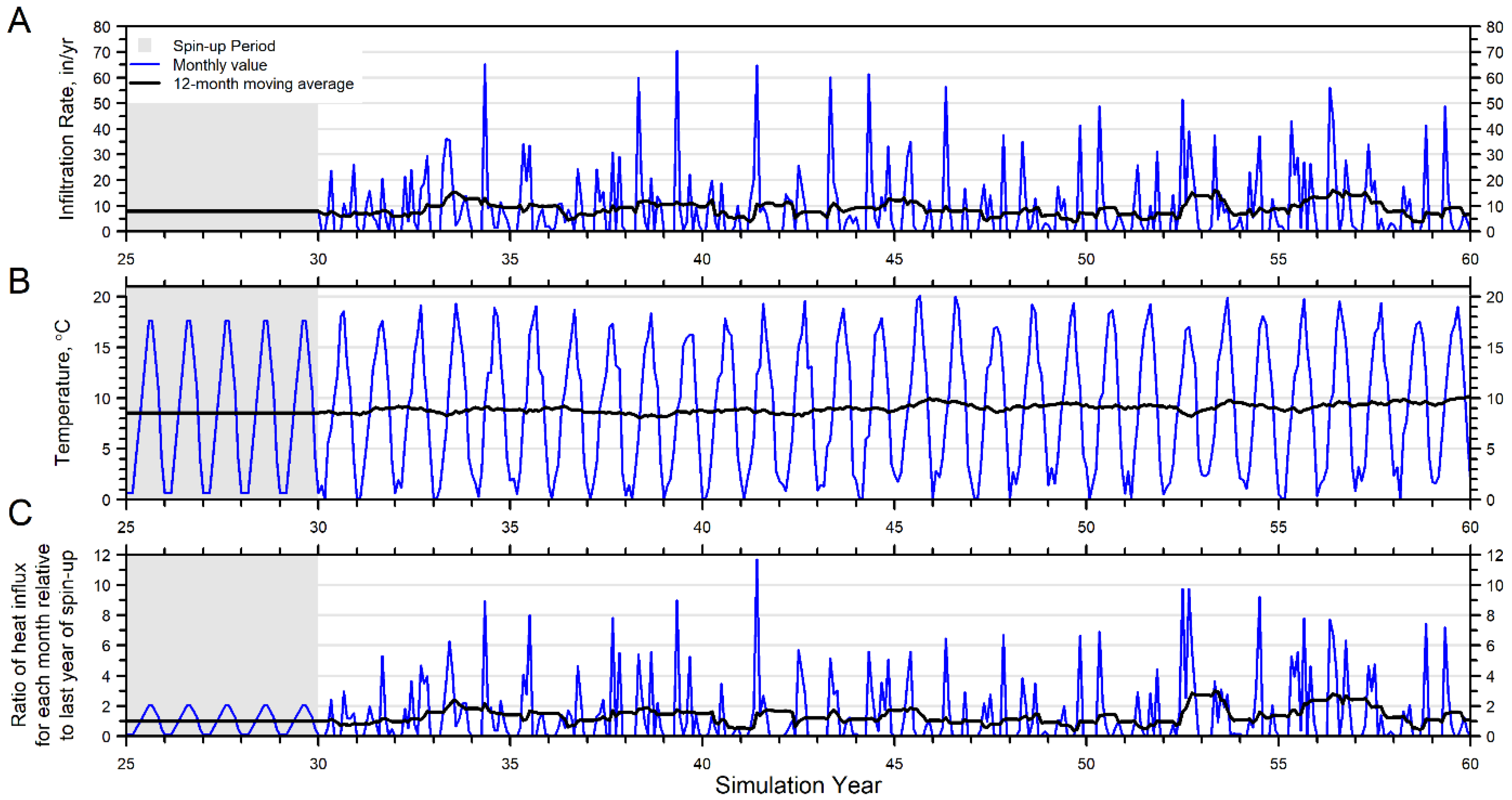
During the 30-year spin-up period, the monthly infiltration rates specified at the top of the UZ total 8.0 in/year (0.20 m/year) and are held constant in each monthly stress period, at 0.66 in/month (0.02 m/month; Figure 1A). In contrast, the infiltration rate varies monthly during the 30-year warm-up period, commensurate with typical seasonal change, but also includes random noise generated from a uniform distribution. The average annual infiltration rate during the 30-year warm-up period is 8.84 in/year (0.224 m/year) and does not include an underlying trend, although the annual totals do vary. The infiltration rates used during the spin-up and warm-up periods are similar to other modeling efforts investigating climate change impacts in humid temperate watersheds, located in Wisconsin, USA [e.g., Table 3 of Hunt et al. (2016) [3]].
During the spin-up period, the temperatures assigned to the monthly infiltration rates vary, but the same sequence of monthly temperatures are repeated every January in order to generate a constant annual average value (Figure 1B). By contrast, the monthly temperatures assigned to the infiltration rates during the 30-year warm-up period reflect three sources of variability: (1) seasonal oscillations, (2) random noise, and (3) an underlying linear warming trend of 0.0025 °C/month (Figure 1B), which equates to 0.9 °C after 30 years, and is commensurate with predicted warming under a high-emission scenario downscaled for southern Wisconsin for the period 2022–2051 [12].
The use of spin-up and warm-up periods results in relative heat influx values that are in a thermal dynamic equilibrium by the end of the spin-up period, and then transition to an unsteady condition during the warm-up period (Figure 1C). Although the warming trend contained within the infiltration temperature time series of the warm-up period is relatively modest, when combined with the variability of the monthly infiltration rates (absent during the spin-up portion of the synthetic simulations), an appreciable increase in the amount of heat added to the system occurs in some stress periods.
The unsteady heat forcing represented in the model during the warm-up period is calculated as the monthly infiltration rate multiplied by the monthly infiltration temperature. The result, after further multiplying by the heat capacity and density of water, results in units of energy/time. Figure 1C shows the ratio of the heat influx for any month, which is calculated as the heat influx for a given month divided by the average heat influx during the last year of spin-up. Hereafter, this ratio is referred to as the relative heat influx. In Figure 1C, seasonal oscillations around a stationary average are present during the spin-up period. During the warm-up period, the relative heat influx shows a considerably more variable pattern. Monthly episodes of significant forcing, or high relative heat influx, are noted throughout Figure 1C, but especially toward the end of the warming period when high monthly infiltration rates are paired with high monthly temperatures (simulation years 52, 55–56; Figure 1C). Additional discussion of the forcing function, and the ramifications of assumptions used to construct them are given in the Supplementary Material Section S1.
2.2. Model Construction: Groundwater Flow
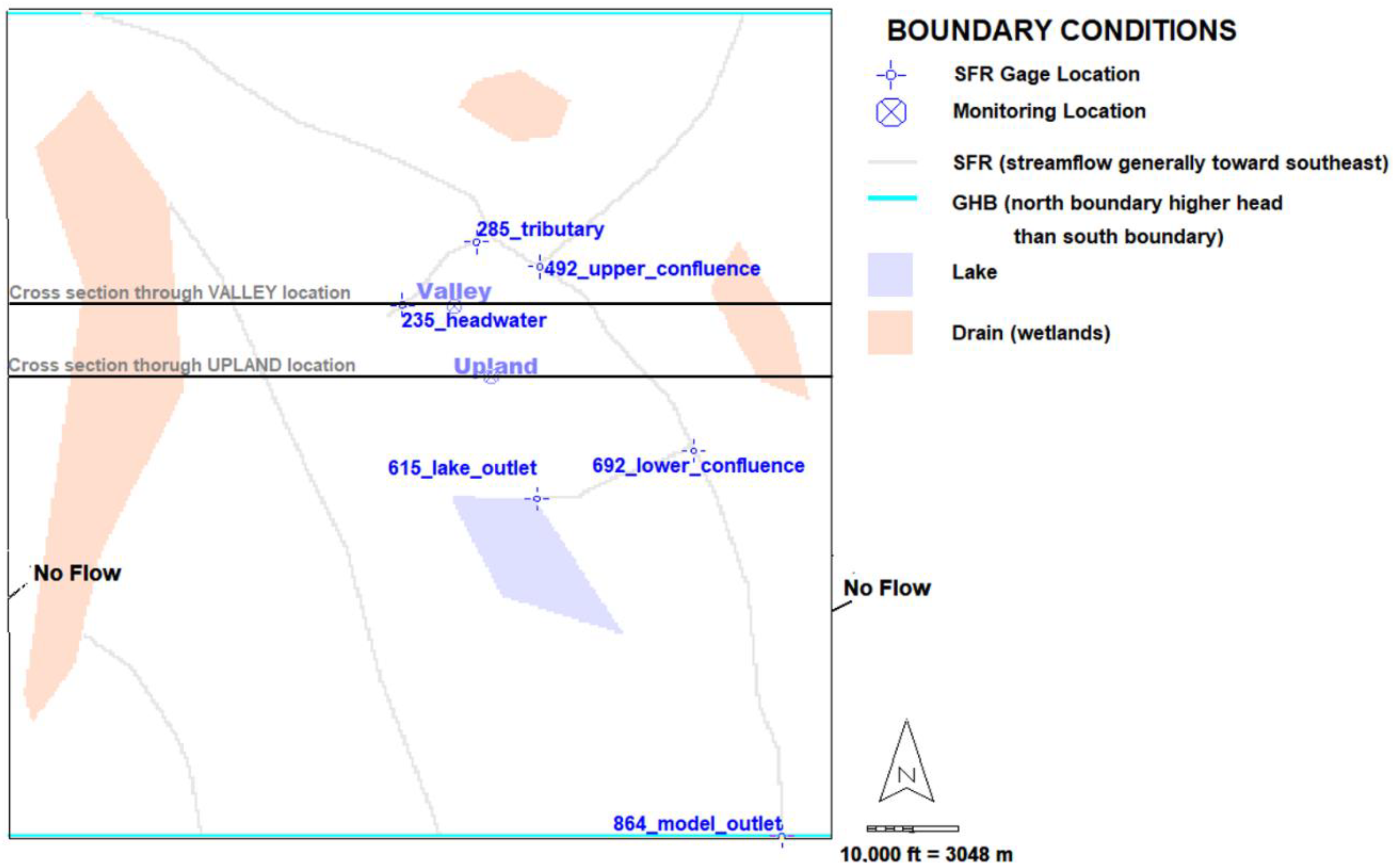
The quasi-hypothetical watershed-scale model covers an area of about 290 square miles (about 750 square kilometers), corresponding in size to a HUC-10 [9] watershed designation (Figure 2). The domain is conceived as a homogeneous (hydraulic conductivity and specific yield) sandy aquifer, with the water table at variable depth below a spatially varying land surface elevation (resulting in variable UZ thickness from cell to cell). The model grid is 300 rows by 300 columns by 8 layers. Laterally, grid cells are 300 ft (91.4 m) on each side and vary in thickness. Aquifer parameters are uniform throughout the domain (Table 1). Boundary condition parameters, controlling sources and sinks of water, are also spatially homogeneous (Table 1).
The General-Head Boundary (GHB) package [10] simulates flow entering the north perimeter boundary and exiting the south perimeter boundary of the model domain. No-flow conditions are imposed along the eastern and western sides of the model at all elevations, and on the bottom of the model. Stream networks are represented by the Streamflow Routing (SFR2) package [13] (Figure 2). Three wetlands are simulated using the Drain (DRN) package [10] and a lake is represented by the Lake (LAK) package [14] (Figure 2). Simulated baseflows within the synthetic model are the sum of (1) direct groundwater discharge to the channel, (2) groundwater discharge to the land surface in riparian areas that subsequently runs off and into the surface-water network, and (3) rejected infiltration resulting from saturation excess in riparian areas that runs off and into the surface-water network. The model is configured so that groundwater–surface-water interaction is one-way as groundwater discharge to the stream; there are no losing reaches. Transient forcing functions and the geometry of surface water sinks, result in appreciable complexity within the flow system, despite the spatially homogeneous parameterization. Additional information on the overarching groundwater model design is provided in Supplementary Material Section S1.
2.3. Representation of Unsaturated Zone Processes
Hunt et al. (2008) [6] demonstrate the importance of including UZ flow processes in steady-state and transient regional-scale groundwater flow models. However, a paucity of data for parameterizing Richards’ equation-based approaches, as well as the computational demands of implementing the approach in numerical models, makes alternative approaches such as that of UZF1, highly attractive [15]. At the time of writing, UZF1 is now a common alternative for simulating UZ flow in regional-scale models [2,3,16,17,18,19,20,21,22]. Hunt et al. (2008) [6] go on to show how UZ flow and the corresponding changes in UZ storage result in lags between the timing of infiltration at the top of the UZ and recharge to the water table. In addition, because of transient water table elevations, the UZ may at times pinch out as the water table rises, resulting in Dunnian overland flow [23]. This, in turn, reduces net infiltration rates which further alters the individual components of a watershed budget. Thus, approaches that omit UZ processes result in infiltration being transmitted instantaneously to the water table at rates that may not be supported by the system. Such over-simplification can confound the use of head data to estimate recharge and can be problematic where timing of infiltration-related recharge is vital for understanding a process of concern (for example, studies involving solute loading to the water table [24] lagged by the unsaturated zone).
Niswonger et al. (2006) [4] offer a detailed explanation of UZF1. Of particular note is that UZF1 neglects capillary forces, an assumption that provides computational efficiencies for regional-scale models [15]. Moreover, UZF1 is equipped to simulate groundwater discharge to land surface when groundwater heads rise to within a user-specified proximity of the land surface [20]. Additionally, UZF1 simulates rejected infiltration when the specified infiltration rate exceeds the vertical hydraulic conductivity (Hortonian overland flow), or when the UZ becomes saturated (Dunnian overland flow). Options are available for routing both the rejected infiltration and groundwater discharge to land-surface to nearby surface water features, which are often important components of the overall water budget [20]. Although supported by the UZF1 package, evapotranspiration was not simulated from the UZ in the synthetic watershed presented herein; rather, evapotranspiration loss is accounted for in the net infiltration rate specified at the top of the UZ. Additional UZF1 information is available in the Supplementary Material Section S1.
Just as with the calculation of infiltration leading to recharge [6], the UZ also acts as a low-pass filter for heat transport, as it migrates downward from near the land surface toward the water table. Equipped with the enhancements described in Morway et al. (2022) [7], MT3D-USGS can simulate heat transport from the top of the UZ, through the UZ and saturated zones, and exchange with surface-water features (represented with different packages). The focus herein is on variably saturated and saturated water temperature, whereas a companion paper focuses on transmission of total energy [25].
Hunt et al. (2008) [6] demonstrated how the thickness of the UZ is a major control on the timing and magnitude of recharge. This investigation goes a step further, and explores how UZ thickness, as well as the parameterization of the UZ, modulate the timing and magnitude of the infiltrating heat signal, prior to becoming recharge. To this end, the synthetic watershed was constructed using three alternative configurations:
- NO_UZ_THK: no UZ processes are simulated by the model. Instead, a monthly infiltration of water and heat is applied directly to the water table, using the Recharge (RCH) [10] and Source/Sink Mixing (SSM) [26] packages, respectively. Note that the NO_UZ_THK and MID_UZ_THK models (explained below) are dimensionally identical (i.e., cell geometries (thicknesses) are the same), meaning that an overlying UZ is present in the NO_UZ_THK, although the grid cells above the water table are inactive. The NO_UZ_THK designation does not imply that the water table is near the land surface throughout the model domain.
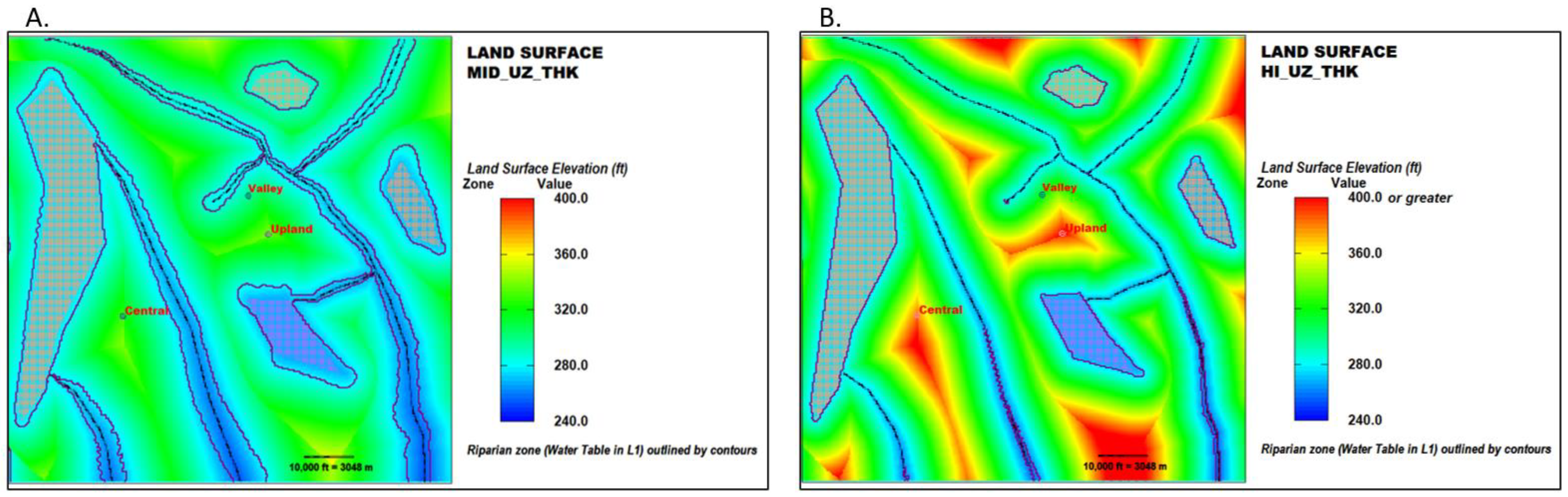
- MID_UZ_THK: a model with the same grid cell dimensions as the NO_UZ_THK simulation but simulates UZ processes with the UZF1 and unsaturated zone transport (UZT) [11,27] packages. The UZ average thickness is approximately 11 ft, with a maximum of 62 ft. The land surface slope from surface water features to “upland” locations is low (1.5 ft/300 ft, or 0.005 ft/ft; Figure 3A).
- HI_UZ_THK: the UZ is approximately three times thicker than the MID_UZ_THK setup, averaging approximately 31 ft thick with a maximum thickness of approximately 150 ft. The land surface slope from surface water features is steeper than the MID_UZ_THK model (3.0 ft/300 ft, or 0.01 ft/ft; Figure 3B).
Differences between the MID_UZ_THK and HI_UZ_THK simulations are evidenced by the water table residing in layer 1 across more than 20% of the MID_UZ_THK simulation domain, while residing only in less than 5% of the layer 1 cells in the HI_UZ_THK simulation (Supplementary Material Section S1).
As with any groundwater solute transport simulation, careful consideration of the model layering (i.e., vertical discretization) scheme is an important part of a heat transport simulation. Too many layers can result in overly lengthy model run-times with untenable linker file [28] sizes that do not offer meaningful gains in simulation accuracy. However, too few model layers can misrepresent heat transport processes, most notably conduction. For example, overly thick grid cells cannot accurately account for thermal gradients that drive conduction and therefore the spread of heat.
The simulations in this analysis use a minimum of eight layers, although sensitivity runs with two additional layers dedicated to the UZ were also explored, using both the MID_UZ_THK and HI_UZ_THK configurations (see Supplementary Material). All models employ a 3 ft thick top layer, referred to below as the “receptor” layer, which functionally serves to receive the heat signal in a spatially consistent manner. The alternative of applying a heat signal to layer 1 cells with spatially varying thicknesses would complicate the interpretation of the relative temperatures in layer 1, since the amount of stored heat would also be a function of the thickness of each cell. Furthermore, keeping layer 1 predominately unsaturated (except when adjacent to surface water features), allows a thermal gradient to develop in the upper UZ for simulating conduction between the UZ layers. The logic for deciding the thickness of layers 2 and 3 was determined after a preliminary run of the model. Both layers were assigned a minimum thickness of 6 ft where the water table reached a minimum depth of less than 15 ft sometime during the simulation (the receptor plus the minimum thickness of 6 ft for layers 2 and 3). Where the minimum water table depth was greater than 15 ft, the thickness of layers 2 and 3 was increased, such that the additional UZ thickness was divided equally among them while layer 1 remained a constant 3 ft thick (see for example Figure S3-2). Where the UZ was greater than 15 ft, the water table resided in layer 4. Layers 5 through 8 were fully saturated for the duration of the simulation and were present to enable differing temperature with depth.
2.4. Model Construction—Heat Transport
The mathematical framework and equations for simulating heat transport in the synthetic watershed discussed herein are presented in detail for a one-dimensional system in Morway et al. (2022) [7]. This study adopts a similar approach but applies the methodology at a watershed scale. Table 2 lists the transport and heat flux parameters applied to all three versions of the model. Heat sorption in the matrix is assumed to act instantaneously, portioning the thermal energy between the solid and fluid phases according to a ratio that varies with water content. The partitioning of the total thermal energy between the aqueous and solid phases is commonly referred to as the retardation factor in MT3D-USGS. A retardation factor of 2.0, for example, implies that half of the thermal energy is “sorbed” to the solid phase, and, therefore, the heat moves at half the advective fluid velocity. For unsaturated flow conditions, the retardation factor depends not only on a linear distribution coefficient, but also on the water content. Additional discussion of the treatment of sorption and the selection of parameter values is provided in the Supplementary Material Section S2.
An aspect of heat transport that is often quite different from solute transport is the relative contribution of the mechanical dispersion and molecular diffusion terms that contribute to the overall hydrodynamic dispersion term. In solute transport, mechanical dispersion is generally orders of magnitude greater than molecular diffusion, especially in advection-dominated settings [29]. In heat transport simulations, however, the thermal conduction as represented by the molecular diffusion term can exceed the mechanical dispersion term. In MT3D-USGS, the thermal conduction is a bulk process, representing the movement of heat fronts through both the solid (not explicitly simulated) and fluid phase [7]. In this modeling exercise, a relatively modest longitudinal dispersivity value of 3 ft is assumed. Although advection in the UZ is downward only, as implemented by the kinematic wave approximation within the UZF1 package, conduction and dispersion may still occur in all directions, including upward, in both the saturated and unsaturated zones (see parameters listed for the DSP Package, Table 2).
Within MT3D-USGS, the streamflow transport (SFT) and lake transport (LKT) packages simulate heat transport in the surface water network, including the exchange of heat between surface water and groundwater [11]. SFT solves a 1D advection-dispersion equation for calculating the temperature within each stream reach. In LKT, a single, instantaneously mixed temperature is calculated for each lake interacting with the aquifer. Groundwater discharged directly to surface water features as well as groundwater runoff (i.e., groundwater discharge to land surface adjacent to streams combined with rejected infiltration from the top of UZ, both instantaneously transferred to the nearest stream or lake feature) is routed through the surface-water network in a way that integrates all upstream discharge for any downstream point. As a result, the stream temperature at a particular location may be realistically simulated as higher or lower than the temperature of the ambient groundwater at that same location. The ability to simulate spatially distributed surface water temperatures at specific points within a watershed is increasingly important for resource management.
3. Results
Simulation results are described here and in the Supplementary Material Section S3. Results are grouped under three main subsections that discuss (1) groundwater temperatures near the water table (where recharge occurs) as they relate to the thickness of the UZ, relative heat influx, and time of year, (2) deeper groundwater temperatures, and (3) the cooling influence of groundwater discharge on surface water temperatures after accounting for the temperature changes occurring in the subsurface.
3.1. Water Table Temperatures
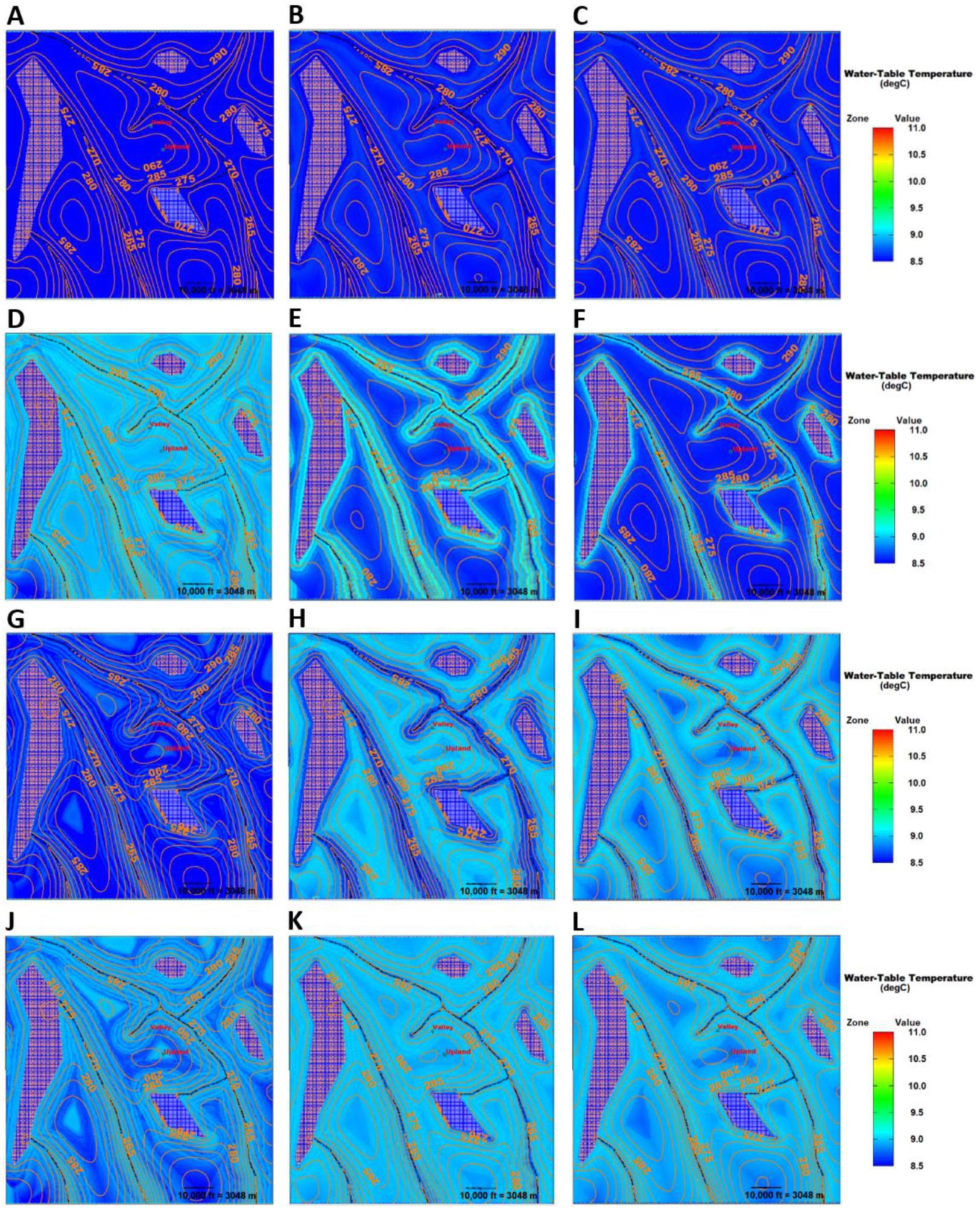
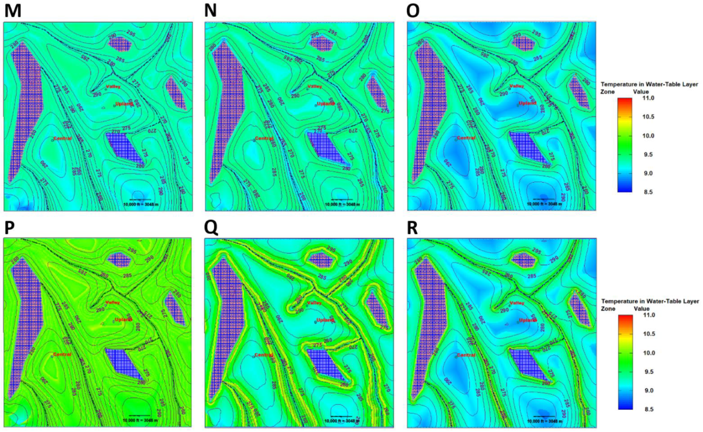
A snapshot of simulated water table temperature for the month of December at the end of the 30-year spin-up period shows nearly identical and uniform conditions of 8.55 °C across all three base models (Figure 4A–C). In the 30 years following the spin-up period (i.e., the warm-up period), the effect of the UZ on the relative heat influx results in a complex spatial and temporal temperature response near the top of the saturated groundwater system, as shown by the monthly snapshots of water table temperatures at 2.75 (Figure 4D–F), 10.17 (Figure 4G–I), 15.17 (Figure 4J–L), 24.67 (Figure 4M–O), and 25.67 years (Figure 4P–R). The relative heat influx ratio for each date displayed in Figure 4 are provided in Table 3. A relative heat influx ratio of 1.0 signifies that the heat loading rate for the month or year, depending on which value is considered, is equivalent to the heat loading rate during the last year of spin-up. In Figure 4D–F, for example, the relative heat loading rate for the second year of the 30-year warm-up period (year 2.75) is 1.30. This suggests that 30% more heat flux (infiltration rate multiplied by the temperature of the infiltration) entered the subsurface, relative to the last year of the spin-up period. In general, the monthly heat flux rates vary by an approximate value of 1.0 over the course of a year, while the annual values gradually increase over the 30-year warming period.
The effect of the UZ is demonstrated by comparing the water table temperature maps for the three test models. For the NO_UZ_THK model (recharge is applied directly to groundwater system rather than routed through the UZ) the map for 2.75 years (September) shows mostly homogeneous water-table conditions, averaging a little above 9 °C early in the warm-up period (Figure 4D). In contrast to Figure 4D, the temperatures in the water table layer of the MID_UZ_THK model (Figure 4E) persist at cooler temperatures (~8.55 °C) where the UZ is thick and are prevalent throughout the model domain at the end of the spin-up period (Figure 4B). However, where the UZ is thin and the infiltration quickly converts to recharge (~1 stress period, equivalent to 1 month), simulated warming at the water table is similar in magnitude to the NO_UZ_THK model, for example along the riparian corridor (Figure 4E). The same is true for the HI_UZ_THK model, except that the effect along the riparian corridors is narrower, due to the steeper slope leading away from the streams and water bodies (Figure 4F).
The expression of warming within a particular model layer depends partly on which month is chosen for closer inspection. For example, after 10.17 years of warm-up (relative heat influx of 1.51), which corresponds to February (relative heat influx of 0.24), the water table temperatures in the NO_UZ_THK model (Figure 4G) remain mostly homogeneous, although the water table temperature has cooled, relative to the temperatures at 2.75 years (Figure 4D). The overall cooling between 2.75 and 10.17 years reflects the direct input of colder water to the water table rather than mixing with warmer water through a thicker UZ, as simulated by the UZT package. For the MID_UZ_THK model (Figure 4H) at 10.17 years, the water table temperatures generally increased from year 2.75. However, the groundwater temperatures are inverted compared to what they were at 2.75 years—the riparian corridor is now cooler than the non-riparian corridor areas (i.e., compare Figure 4E to Figure 4H). Similar temperatures are exhibited in the HI_UZ_THK model (i.e., compare Figure 4F to Figure 4I). In another February snapshot from five years later (15.17 years; Figure 4J–L), all three models show similar patterns, as seen at 10.17 years of generally warmer water table temperatures, because the warming trend applied to the temperature of the infiltration begins to affect the overall ambient temperature of the water table.
At 24.67 years into warming, corresponding to August, the NO_UZ_THK and MID_UZ_THK results (Figure 4M,N) show a similar and fairly uniform water table temperature across the model domain. For the same simulated period, the water table temperatures in the HI_UZ_THK model (Figure 4O) appreciably depart from the NO_UZ_THK and MID_UZ_THK model results. That is, the water table temperature is less uniform—areas below a thicker UZ are cooler, for example, at the UPLAND location. The final set of water table temperature maps (Figure 4P–R), also corresponding to August, show the groundwater temperature at 25.67 years. This period is characterized by the highest monthly relative heat influx during the entire warming period (7.79; Figure 1C) as well as a very high average annual relative heat influx (2.12). The NO_UZ_THK model shows warmer temperatures over most of the domain, at nearly 10 °C (Figure 4P). In contrast, the MID_UZ_THK model shows warmer riparian corridors and cooler temperatures under the uplands (Figure 4Q). The HI_UZ_THK model for year 25.67 (Figure 4R) is cooler under the uplands and along the river corridors than either of the other two models. A comparison of the water table temperatures after 24.67 and 25.67 years of warming shows that appreciable warming occurred during the elapsed year in the NO_UZ_THK and MID_UZ_THK models (i.e., comparing Figure 4M to Figure 4P, and Figure 4N to Figure 4Q, respectively) and only a small amount of warming in the HI_UZ_THK model (i.e., comparing Figure 4O to Figure 4R). Given that the only difference between these models is the thickness of the UZ, the cooler temperatures in the HI_UZ_THK model suggest meaningful thermal buffering in the UZ before infiltrating heat reaches the water table.
3.2. Groundwater System Temperatures
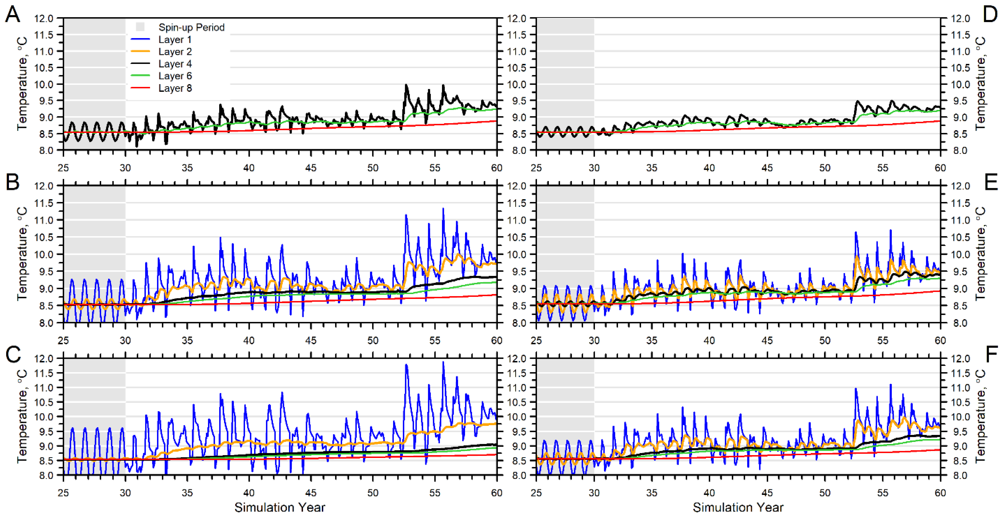
Time series plots of the simulated temperature at the UPLAND location show markedly different behavior for each layer of the three base models (Figure 5). For example, the temperature response in the water table layer (layer 4) of the NO_UZ_THK model exhibits higher frequencies and amplitudes compared with the MID_ and HI_UZ_THK models. This result is expected, since the UZ is not simulated and therefore unable to buffer the infiltrating heat signal. Thus, the layer 4 response at the UPLAND location is notably flashier in the NO_UZ_THK model (Figure 5A). The temperature response in layer 4 for the other two models with thicker unsaturated zones is much smoother, and the total warm-up in layer 4 of the MID_UZ_THK (Figure 5B) model is approximately 0.3 °C less by the end of the simulation, compared with the HI_UZ_THK model (Figure 5C). The simulated temperatures also trend upward at the VALLEY location in all layers Figure 5D–F), albeit with different behaviors. For example, the amplitude of the temperature swings in layer 1 at the UPLAND location is greater than at the VALLEY location; however, larger amplitudes are seen at the VALLEY location in layers 2 and 4, compared with the UPLAND location. Additional cross-sectional results are provided in the Supplementary Material Section S3.
3.3. Stream Baseflow Temperatures
Groundwater discharge plays an import role in cooling streamflow temperatures, particularly during late summer, when its proportional contribution to streamflow is greatest (i.e., baseflow conditions). Because groundwater discharge is comprised of an ensemble of subsurface flow paths, streamflow temperature during baseflow largely reflects the (1) thermal buffering that occurred within the UZ prior to the infiltrating water becoming recharge, (2) buffering within the saturated zone as groundwater flow paths of different temperature converge, (3) thermal buffering that occurred within the UZ prior to it becoming recharge, and (4) other processes not specifically addressed in this paper, including direct atmospheric effects on surface water. Heat in storm runoff from the land surface, not addressed here but incorporated in a companion paper by Feinstein et al. (2022) [25], does not affect baseflow temperatures, but rather acts on total streamflow temperatures. The key point is that simulated baseflow temperatures for a given location within a stream network represent a composite of heat accumulated from upstream in the watershed. In particular, the baseflow temperature responds to dampened heat flows through the UZ and the saturated system, along with the undampened heat contribution from groundwater runoff (by way of rapid transfers from groundwater discharge to the land surface plus rejected infiltration from the top of the unsaturated zone).
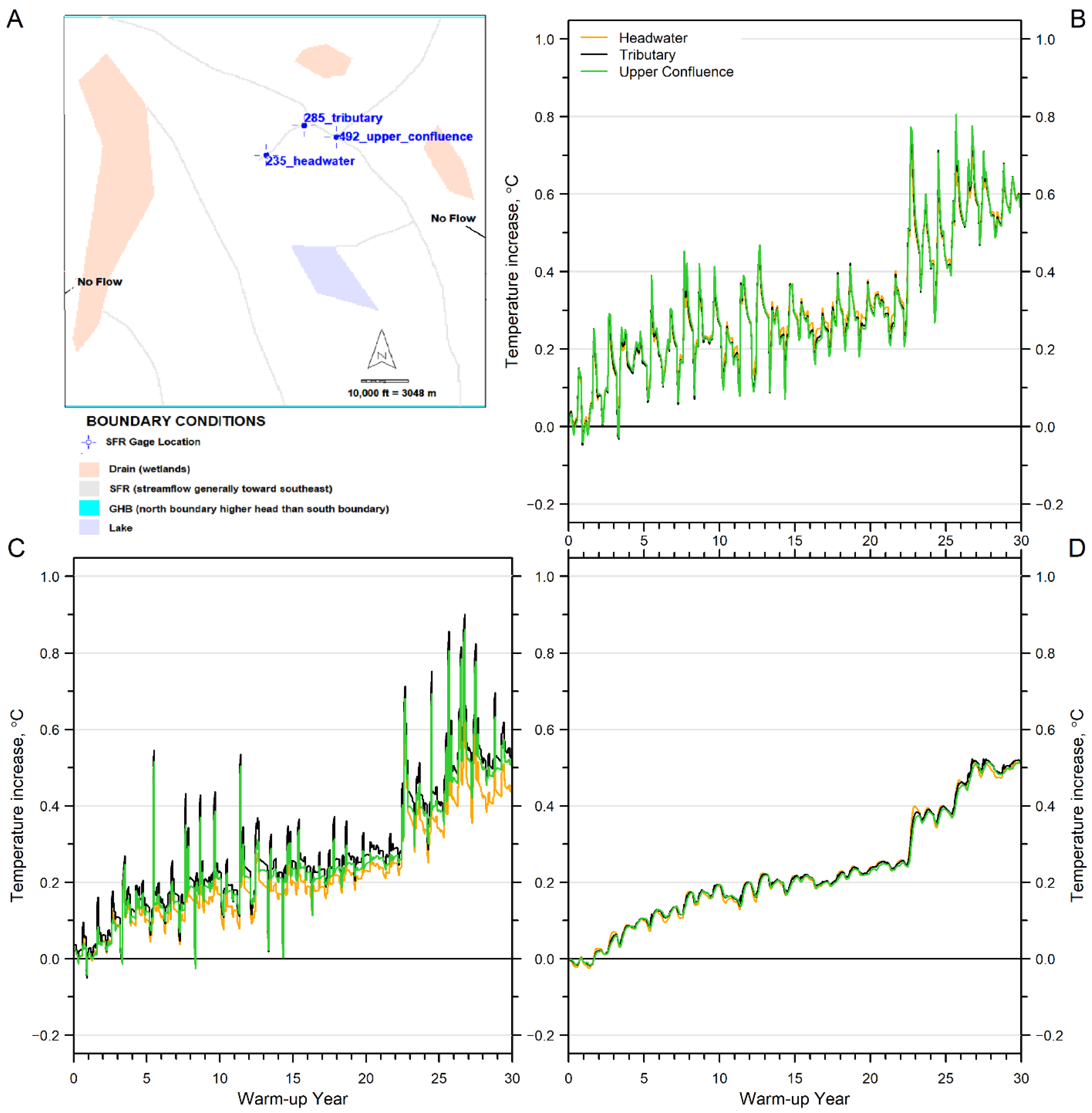
The hypothetical stream gage locations used in this investigation to describe baseflow conditions are divided into two groups of three (Figure 6): the first group consists of upgradient gages (Figure 2) corresponding to a headwater location (site 235), a tributary outlet (site 285), and an upper confluence location (site 492), while the second group of downgradient gages consists of a lake outlet (site 615), a lower confluence (site 692), and the model outlet (site 864). Temperatures in the lake outlet gage reflect a single temperature computed for a well-mixed lake through time. Temperatures at the model outlet gage reflect the integrated response of an entire upgradient surface-water network over time.
For the upgradient gages, results of the NO_UZ_THK model (Figure 6B) show a seasonal temperature frequency and a rising magnitude trend, but with little temperature separation at the three gage locations (Figure 6A). The MID_UZ_THK model (Figure 6C) shows seasonality and rising trends in stream temperatures similar to the NO_UZ_THK model (Figure 6D), but with increased separation among the thermal hydrographs. For example, the 95th percentile temperature increase is greatest at the tributary location and lowest at the upstream headwater location. In contrast to the other simulations, stream temperatures generated by the HI_UZ_THK model are virtually identical across the three upgradient locations, and the upward trend is notably dampened, compared with the NO_UZ_THK and MID_UZ_THK models.
For the three downgradient gage locations (Figure 7A), the streamflow temperature response is different from that of the upgradient locations. For example, in all three test models, the lake outlet gage (Figure 7A) shows a pronounced yearly oscillation superimposed on the rising trend. Although the codes used in this work do not simulate all components of the lake temperature budget, the lake outlet results have heuristic value. Annual temperature swings of roughly 0.3 °C are simulated at the lake outlet, where the lake acts as a well-mixed reservoir, integrating discharge from its groundwater contributing area, which largely consists of areas with little UZ thickness. That is, the simulated streamflow temperature at the lake outlet reflects the solitary temperature simulated for the entire lake. The lower confluence location (ID 692) is somewhat dampened for all three base model versions. However, the results at the model outlet gage are less flashy in the NO_UZ_THK model (Figure 7B) compared to the flashier temperatures in the MID_UZ_THK model (Figure 7C), with the 95th percentile stream baseflow temperature increase for the moderately thick UZ model exceeding 0.6 °C, and an excursion (maximum minus minimum) exceeding 1.0 °C. Results of the HI_UZ_THK model (Figure 7D), by contrast, show a dampened response in the streams for both the lower confluence and model outlet locations.
For the NO_UZ_THK and MID_UZ_THK simulations, the flashiest stream temperature response is at the model outlet gage (Figure 7B,C respectively)—an initially counterintuitive result, considering that this location integrates contributions from the largest portion of the watershed. However, because the model outlet is flanked by riparian areas (the water table resides in the top 3-foot-thick layer), there is minimal UZ buffering for the MID_UZ_THK model, and no buffering for the NO_UZ_THK model; therefore, direct runoff contributed by precipitation will immediately (that is, within the same model monthly time step) influence the stream temperature. The extent of the riparian area varies within the contributing area of each gage, where a rough trend of increasing riparian area at more downstream gage locations is observed (Table 4). For the NO_UZ_THK model, the specified recharge volumes (as opposed to simulating infiltration with UZF) result in elevated water levels near the streams and (unrealistic) high groundwater gradients, which, in turn, facilitate rapid lateral groundwater flow to nearby streams that discharge appreciable amounts of flow and heat in a short period of time. In the MID_UZ_THK model, an extensive riparian area exists within the contributing area, that is, between the lower confluence (gage 692) and model outlet (gage 864). In this circumstance, a thin UZ associated with a water table near the land surface facilitates rejected infiltration; that is, the ability of the groundwater system to accept infiltration is significantly reduced and it is therefore shunted as runoff to the nearby stream. Conversely, the reduced riparian area in the HI_UZ_THK simulation, along with more dampening of a thick UZ, results in a smoother stream temperature response.
By the end of the 30-year warm-up period (i.e., the end of the simulations), an overall increase in the stream baseflow temperature of approximately 0.5 °C is simulated at all three of the downgradient gage locations (Figure 7). This increase is roughly half of the 1.0 °C rise in the simulated water table temperature at the VALLEY well location (the shallowest layer for each UZ model; Figure 5D–F), an area with a similarly shallow water table. Thus, there is a thermally dampened response in the stream temperatures relative to the groundwater system, which is suggestive of groundwater mixing—the upwelling of cooler groundwater from deeper groundwater flow paths combining with shallower and warmer flow paths—before discharging into the stream. It is important to emphasize that at the end of the 30-year warm-up period, simulated temperatures throughout the system have not reached a new dynamic equilibrium. In other words, the UZ continues to buffer the underlying warming signal applied to the infiltration during the last 30 years of the simulation. Additionally, cooler groundwater from deeper parts of the aquifer mixes with the warmer groundwater near the water table to further dampen the effect of the warming signal on the stream temperatures. Finally, longer flow paths, unaffected by 30 years of warming, may begin to show signs of more significant warming, given enough time. For example, the simulated groundwater temperatures in layer 8 do show signs of warming by the end of the simulations (Figure 5), although it is the most muted response across all layers. Therefore, the overall watershed residence time, and the distribution of residence times within a watershed, influence the thermal resiliency of a watershed subject to warming.
Additional UZ layers for further resolving UZ flow and transport had little effect on the final temperatures, indicating that the kinematic wave approximation within the UZF1 package provides sufficient information to capture lags in the infiltrating heat flux. However, including at least one completely unsaturated layer above the water table enables MT3D-USGS to simulate lags in heat reaching the water table, since MT3D-USGS instantaneously mixes the unsaturated and saturated temperatures (i.e., “concentrations”) in cells containing the water table [11]. A parameter sensitivity analysis (Supplementary Material Section S3) showed that the simulated water table temperatures responded more strongly to perturbations than the stream temperatures. Table S3-1 lists the parameters that were adjusted. Parameters related to flow of water (UZ vertical hydraulic conductivity and saturated water content) had modest sensitivity, while heat transport-related parameters (i.e., distribution coefficient, thermal conductivity) were more sensitive. However, a highly reduced UZ vertical hydraulic conductivity did appreciably reduce the amount of groundwater recharge, which was balanced by an increase in rejected infiltration, leading to an increase in the amount of overland flow to surface water, which in turn affected the heat balance of the system.
4. Discussion and Implications for Watershed Heat Transport Modeling
The simulated temperatures throughout the watershed may be evaluated in terms of how the infiltrating heat signal’s amplitude, frequency, and phase are modified first by the UZ, and secondly by the saturated zone. For example, seasonal swings in the average simulated temperature of layer 1 can be as high as 2.5 °C (Figure 5B,C,E,F), although they are frequently less than that. When the heat signal reaches the bottom of the UZ (represented by layers 1–3), the amplitudes of the seasonal swings in temperatures have almost entirely disappeared, although small seasonal swings in the groundwater temperature are still evident at the VALLEY location in layer 4 of the MID_UZ_THK simulation (Figure 5E). The existence of some seasonality in temperature for layer 4 in the MID_UZ_THK model (Figure 5E) compared with the HI_UZ_THK model (Figure 5F) further demonstrates the dampening effect of the UZ. Thus, the temperature swings assigned to the infiltration at the top of the UZ (Figure 1) are largely smoothed by the unsaturated and saturated zones.
By the end of the warm-up period, the simulated average temperature increase in layer 4—representative of the shallow part of the groundwater system—is approximately 0.75 °C at the UPLAND location in the MID_UZ_THK model (Figure 5B). At the VALLEY location, the average temperature of layer 4 increased by nearly 1.0 °C (Figure 5E). The average temperature increase in the deeper aquifer, represented by layer 8, was only approximately 0.25 °C and 0.40 °C at the UPLAND (Figure 5B) and VALLEY (Figure 5E) locations, respectively, in the MID_UZ_THK model. In general, layer 8 is representative of groundwater temperatures roughly 100 ft (30 m) below the water table.
The behavior of stream baseflow temperatures during warming is shown for downstream gages in Figure 7. At the end of the 30-year warm-up period, the stream temperatures rose between 0.5–0.6 °C in the three models, compared with the end of the spin-up period. Thus, the model, as expected, simulates less overall warm-up in the stream temperatures compared with the amount of warm-up applied to the infiltrating water (2 °C, Figure 1B). The dampened stream temperature response is sustained by the discharge of colder groundwater from deeper in the aquifer mixing with the groundwater discharge. Moreover, the effect of UZ thickness on stream temperatures also is likely evident in the results; for the upgradient locations, the HI_UZ_THK stream temperatures (Figure 6D) are much smoother and considerably more muted, compared with the MID_UZ_THK stream temperatures (Figure 6C).
A final consideration in evaluating infiltrating heat in a watershed is the phase, or lag time, between the forcing boundary condition (i.e., the temperature of the infiltration) and the downgradient response. The effects of lag time are most clearly seen during periods of high heat inflow, where the response is felt relatively quickly in the MID_UZ_THK simulation (i.e., warmer temperatures below the UPLAND area in Figure 4Q), whereas cooler temperatures persist for the same location in the HI_UZ_THK simulation (Figure 4R).
These findings have implications for watershed heat transport simulations in humid temperate climates. They are:
- A potential effect of warming climate on groundwater temperatures in a watershed depends on the relative heat flux—the product of infiltration rate and associated temperature—that determines the amount of heat entering the subsurface. For example, if the temperature of infiltrating water increases during a warming climate, the net change in groundwater temperature may be lessened if drought conditions cause the rate of infiltration to be reduced;
- The UZ acts as a low-pass filter. Both the magnitude and timing of water and heat pulses entering the subsurface and migrating downward to the water table, are attenuated by the UZ. Neglecting the UZ from a model simulation (as in the NO_UZ_THK version of the synthetic model) effectively “short circuits” the dampening and lag time influences of the UZ;
- The effect of a warming climate is buffered in a watershed by the total thickness of the groundwater system. A relatively thick groundwater system gives rise to mixed water temperatures at natural discharge points where shallow and deep flow lines converge. The convergence of flow lines dampens the heat signal carried by recharge that eventually discharges as baseflow to surface water;
- The spatial extent of riparian zones plays an important role in determining the flashiness of a stream’s response to heat forcing. That is, the riparian zone sheds (or shunts) precipitation to the surface water network, without the low-pass filtering of the UZ;
- Additional vertical discretization to more accurately simulate the movement of wetting and heat fronts did not change simulation results. However, omission of the UZ and its effects on heat transport in a watershed-scale model produces erroneous results;
- A sensitivity analysis of the flow and heat transport parameters showed an appreciable influence on simulated temperatures in both the saturated and unsaturated components of the subsurface, as well as on simulated stream temperatures (Supplementary Material Section S3).
5. Limitations of the Methodology
A discussion of the limitations and assumptions used in this work are provided in Supplementary Material Section S3, with a brief summary here.
- Root zone processes (i.e., evapotranspiration) are neglected; therefore, the infiltration rate is equated with the water that drains out of the root zone and enters the top of the UZ.
- As noted above, the UZF1 package in MODFLOW implements simplifying assumptions that neglect capillary forces. As a result, UZF1 simulates downward-only gravitational flow. This simplification is generally considered acceptable at a watershed scale [30].
- With the UZF1 package active in MODFLOW, one of three potential states is simulated for any active cell. They are either (1) unsaturated (i.e., partially-saturated over the entire thickness of the active grid cell), (2) a mix of unsaturated and saturated conditions (i.e., the water table is present within the cell), or (3) fully saturated. For water table cells, a single water content value is calculated that is equivalent to a volume average of both the unsaturated and saturated portions of the cell. Ambiguity arising from this mixed condition appears to have minimal effect on the heat flux solution, insofar as refined layer discretization hardly changes model results (Supplementary Material Section S3).
- Although conduction occurs through the matrix material of an aquifer and may transport heat more rapidly than in the fluid phase in low convection environments, MT3D-USGS simulates a single “bulk” diffusion term that approximates heat transport through both phases. In other words, the conductive propagation of heat through the solid and fluid phases is represented as a conjoined movement that is slower than thermal diffusion through a pure solid but faster than thermal diffusion through a pure fluid. In a predominantly horizontal flow-field, the upward or downward thermal diffusion is generally secondary, compared with the convection in humid temperate climates [25]. It is conceivable that the conductive flux through matrix material is dominant when the temperature gradient is unusually strong.
- The methods applied in this study were designed for temperate climate regions. It neglects processes such as mountain-front recharge in settings with deep water tables (>30 m), long flow paths (>2–3 km), and long UZ residence times, which are characteristic of arid and semi-arid regions.
- The effects of changes in viscosity owing to temperature changes are not considered in this study. However, variations in viscosity over the relatively small temperature changes simulated in the model are expected to be small.
A second group of limitations that are not related to the methodology chosen, but instead arise from the way the synthetic watershed model was constructed, include:
- Temporal smoothing of system dynamics via the use of a monthly climate forcing.
- Simplification of the thermal influence of storm runoff to streams was ignored/not simulated: that is, the restriction of the simulation to monthly average baseflow conditions.
- Inadequate representation of lake energy budget considerations as important for lake temperature. For example, neglecting the formation of ice during the winter months, energy changes related to evaporation, and lake thermal stratification.
Finally, it is important to note that the heat forcing function used to represent watershed warming in this study was designed to illustrate the components of watershed heat transport rather than represent an expected future condition. A companion paper, Feinstein et al. (2022) [25], incorporates a heat forcing function derived from predictions of climate trends.
6. Conclusions
This study developed a methodology for simulating watershed scale heat transport in a humid temperate climate. Beyond the use of the modified MT3D-USGS code described in Morway et al. (2022) [7], the applied methodology relies on two aspects of the model design:
- Whereas specification of infiltration is critical for representative groundwater flow models, specification of the heat forcing function, represented by the product of the infiltration rate added to the top of UZ multiplied by the infiltration temperature (the relative heat influx) is critical for developing a representative heat transport model.
- Heat transport in watershed models stand to benefit from a discretization scheme with at least one unsaturated layer. This approach enables the simulation to store, dampen, and/or lag the heat pulse before it is mixed with an underlying water table cell.
By the end of each simulation, the increase in the stream baseflow temperature (approximately 0.5 °C) is approximately half of the temperature increase at the water table (approximately 1.0 °C). Even with simulating monthly average conditions, the spatial extent of the riparian zone (water table < 1 m deep) plays an important role in determining the temperature ‘flashiness’ of the stream response to heat forcing. Thin UZs in riparian areas are more likely to generate rejected infiltration (runoff), which effectively short-circuits the dampening effects of a thicker UZ.
The methods applied in this study of a synthetic watershed highlight the importance of including the UZ in heat transport models. The UZ acts a low-pass filter that dampens the simulated effect of an infiltrating heat signal over time. That is, the thickness of the UZ can modify the amplitude, frequency, and phase change of the infiltrating heat signal as it migrates down to the water table. Moreover, because the thickness of the UZ varies across the active model domain, explicit representation of the UZ within a watershed model better captures the spatially-varying effect of the UZ on heat fluxes delivered to the water table. Equipped with a spatially and temporally refined recharging heat flux simulated by the model, the subsequent heat-buffering effects of the groundwater (saturated) system on a migrating heat signal are better accounted for. For example, as the shallow and deep flow paths converge near discharge points, the respective temperatures associated with each flow path mix. In this way, the cumulative and combined effects of the unsaturated and saturated zones on the temperature of the discharge to surface water features is more accurately simulated. Thus, heat transport models that consider the unsaturated and saturated zones are better equipped to evaluate the impacts of a changing climate on ecologically sensitive endpoints such as stream habitats.
Supplementary Materials
The following supporting information can be downloaded at https://www.mdpi.com/article/10.3390/w14233883/s1. Figure S1-1: Monthly and average yearly infiltration rates over warming period; Figure S1-2: Average yearly infiltration rate over warming period; Figure S1-3: Monthly temperature signal for spin-up; Figure S1-4: Forcing function component: Monthly temperature; Figure S1-5: Forcing function component: Relative monthly heat influx; Figure S1-6: Relative heat influx: 12-month averages during warming; Figure S1-7: Average relative heat influx by month for 30-year spin-up and 30-year warming; Figure S1-8: Synthetic model; Figure S1-9: Model layering and water-table elevation for UPLAND and VALLEY locations at end of spin-up period; Figure S1-10: Depth to water table at end of spin-up; Figure S2-1: Linear relations between thermal conductivity and volumetric moisture content; Figure S3-1: Head hydrographs for base model layers 1-8 at UPLAND and VALLEY locations; Figure S3-2: Temperature and water-table elevation in cross section through UPLAND location for three base models, layers 1-8, at selected times during warming period; Figure S3-3: Stream baseflow temperature for three base models in response to warming at selected gages; Figure S3-4: Cross sections showing layering for 8-layer base model version and 10-layer revised base model version of MID-UZ-THK; Figure S3-5: Cross sections showing layering for 8-layer base model version and 10-layer revised base model version of HI-UZ-THK; Figure S3-6: Temperature hydrographs comparing results for 8-layer and 10-layer model versions for the UPLAND location; Figure S3-7: Temperature hydrographs comparing results for 8-layer and 10-layer model versions for VALLEY location; Figure S3-9: Sensitivity results for MID_UZ_THK model as a percentage of model domain for August, by year, with water-table temperature at or above 9.5°C; Figure S3-10: Sensitivity results for MID_UZ_THK model for stream temperatures at the model outlet gage during warming period; Table S1-1: Infiltration rates over warming period in inches/year; Table S1-2: Vertical distribution of water-table elevations and corresponding temperatures at selected times during warming. Units for average temperature are degrees Celsius; Table S2-1: Spatially homogeneous transport and heat flux parameters; Table S3-1: Summary of changes to parameter values for sensitivity simulations using the MID_UZ_THK base model. References [31,32,33,34] at the end of the reference list are cited in the Supplementary Materials.
Author Contributions
E.D.M., D.T.F. and R.J.H. shared equally in the conceptualization of the material.; E.D.M. and D.T.F. split much of the writing, with help from R.J.H.; E.D.M. and D.T.F. collaborated on the figures; E.D.M. took the lead on the response to reviewers, with contributions from coauthors. All authors have read and agreed to the published version of the manuscript.
Funding
The authors would like to acknowledge support from the U.S. Geological Survey Land Change Science/Climate Research and Development for this work.
Data Availability Statement
The model executables, input and output files associated with the example models described in this manuscript are available in an online model archive located at: https://doi.org/10.5066/P99NUKIX (Morway et al., 2022b) [35].
Acknowledgments
Any use of trade, firm, or product names is for descriptive purposes only and does not imply endorsement by the U.S. Government. The authors wish to thank Dan Bright and Ramon Naranjo, both from the U.S. Geological Survey’s Nevada Water Science Center, as well as anonymous reviewers selected by the journal, for their helpful reviews.
Conflicts of Interest
The authors declare no conflict of interest.
References
- IPCC. Climate Change 2022: Impacts, Adaptation, and Vulnerability, Technical Summary; Cambridge University Press: Cambridge, UK, 2022. [Google Scholar]
- Hunt, R.J.; Walker, J.F.; Selbig, W.R.; Westenbroek, S.M.; Regan, R.S. Simulation of Climatechange Effects on Streamflow, Lake Water Budgets, and Stream Temperature Using GSFLOW and SNTEMP, Trout Lake Watershed, Wisconsin; U.S. Geological Survey Scientific Investigations Report 2013-5159; U.S. Geological Survey Scientific: Reston, VA, USA, 2013; p. 118. Available online: http://pubs.usgs.gov/sir/2013/5159/ (accessed on 15 January 2022).
- Hunt, R.J.; Westenbroek, S.M.; Walker, J.F.; Selbig, W.R.; Regan, R.S.; Leaf, A.T.; Saad, D.A. Simulation of Climate Change Effects on Streamflow, Groundwater, and Stream Temperature Using GSFLOW and SNTEMP in the Black Earth Creek Watershed, Wisconsin; 2328-0328; U.S. Geological Survey, Scientific Investigations Report 2016-5091; U.S. Geological Survey Scientific: Reston, VA, USA, 2016; p. 117. [CrossRef]
- Niswonger, R.G.; Prudic, D.E.; Regan, R.S. Documentation of the Unsaturated-Zone Flow (UZF1) Package for Modeling Unsaturated Flow between the Land Surface and the Water Table with MODFLOW-2005; 2328-7055; U.S. Geological Survey Scientific: Reston, VA, USA, 2006; p. 62. [CrossRef]
- Niswonger, R.G.; Panday, S.; Ibaraki, M. MODFLOW-NWT, a Newton Formulation for MODFLOW-2005; U.S. Geological Survey Scientific: Reston, VA, USA, 2011; p. 44. [CrossRef] [Green Version]
- Hunt, R.J.; Prudic, D.E.; Walker, J.F.; Anderson, M.P. Importance of unsaturated zone flow for simulating recharge in a humid climate. Groundwater 2008, 46, 551–560. [Google Scholar] [CrossRef]
- Morway, E.D.; Feinstein, D.T.; Hunt, R.J.; Healy, R.W. New capabilities in MT3D-USGS for Simulating Unsaturated-Zone Heat Transport. Groundwater 2022. [Google Scholar] [CrossRef] [PubMed]
- Anderson, M.P.; Bowser, C. The role of groundwater in delaying lake acidification. Water Resour. Res. 1986, 22, 1101–1108. [Google Scholar] [CrossRef]
- USDA-NRCS. HUC10: USGS Watershed Boundary Dataset of Watersheds. Available online: https://datagateway.nrcs.usda.gov (accessed on 25 May 2022).
- Harbaugh, A.W. MODFLOW-2005, the U.S. Geological Survey Modular Ground-Water Model: The Ground-Water Flow Process; U.S. Geological Survey Scientific: Reston, VA, USA, 2005. [CrossRef] [Green Version]
- Bedekar, V.; Morway, E.D.; Langevin, C.D.; Tonkin, M.J. MT3D-USGS Version 1: A U.S. Geological Survey Release of MT3DMS Updated with New and Expanded Transport Capabilities for Use with MODFLOW; 2328-7055; U.S. Geological Survey Scientific: Reston, VA, USA, 2016. [CrossRef] [Green Version]
- USGS. National Climate Change Viewer. Available online: https://www2.usgs.gov/landresources/lcs/nccv/maca2/maca2_watersheds.html (accessed on 31 January 2022).
- Niswonger, R.G.; Prudic, D.E. Documentation of the Streamflow-Routing (SFR2) Package to Include Unsaturated Flow Beneath Streams—A Modification to SFR1; 2328-7055; U.S. Geological Survey, Techniques and Methods 6-A13; U.S. Geological Survey Scientific: Reston, VA, USA, 2005. [CrossRef] [Green Version]
- Merritt, M.L.; Konikow, L.F. Documentation of a Computer Program to Simulate Lake-Aquifer Interaction Using the MODFLOW Ground-Water Flow Model and the MOC3D Solute-Transport Model; U.S. Geological Survey Water-Resources Investigations Report 00–4167; U.S. Geological Survey Scientific: Reston, VA, USA, 2000; p. 146. Available online: https://pubs.er.usgs.gov/publication/wri004167 (accessed on 15 May 2020).
- Niswonger, R.; Prudic, D.E. Comment on “evaluating interactions between groundwater and vadose zone using the HYDRUS-based flow package for MODFLOW” by Navin Kumar, C. Twarakavi, Jirka Simunek, and Sophia Seo. Vadose Zone J. 2009, 8, 818–819. [Google Scholar] [CrossRef]
- Markstrom, S.L.; Niswonger, R.G.; Regan, R.S.; Prudic, D.E.; Barlow, P.M. GSFLOW-Coupled Ground-Water and Surface-Water FLOW Model Based on the Integration of the Precipitation-Runoff Modeling System (PRMS) and the Modular Ground-Water Flow Model (MODFLOW-2005); U.S. Geological Survey Techniques and Methods 6-D1; U.S. Geological Survey Scientific: Reston, VA, USA, 2008; p. 240. Available online: https://pubs.usgs.gov/tm/tm6d1/pdf/tm6d1.pdf (accessed on 15 May 2020).
- Morway, E.D.; Gates, T.K.; Niswonger, R.G. Appraising options to reduce shallow groundwater tables and enhance flow conditions over regional scales in an irrigated alluvial aquifer system. J. Hydrol. 2013, 495, 216–237. [Google Scholar] [CrossRef]
- Woolfenden, L.R.; Nishikawa, T. Simulation of Groundwater and Surface-Water Resources of the Santa Rosa Plain Watershed, Sonoma County, California; 2328-0328; U.S. Geological Survey, Scientific Investigation Report 2014-5052; U.S. Geological Survey Scientific: Reston, VA, USA, 2014. [CrossRef] [Green Version]
- Haserodt, M.J.; Hunt, R.J.; Fienen, M.N.; Feinstein, D.T. Groundwater/Surface-Water Interactions in the Partridge River Basin and Evaluation of Hypothetical Future Mine Pits, Minnesota; 2328-0328; U.S. Geological Survey, Scientific Investigations Report 2021-5038; U.S. Geological Survey Scientific: Reston, VA, USA, 2021. [CrossRef]
- Feinstein, D.T.; Hart, D.J.; Gatzke, S.; Hunt, R.J.; Niswonger, R.G.; Fienen, M.N.J.G. A simple method for simulating groundwater interactions with fens to forecast development effects. Groundwater 2020, 58, 524–534. [Google Scholar] [CrossRef] [PubMed] [Green Version]
- Khadim, F.K.; Dokou, Z.; Bagtzoglou, A.C.; Yang, M.; Lijalem, G.A.; Anagnostou, E. A numerical framework to advance agricultural water management under hydrological stress conditions in a data scarce environment. Agric. Water Manag. 2021, 254, 106947. [Google Scholar] [CrossRef]
- Kitlasten, W.; Morway, E.D.; Niswonger, R.G.; Gardner, M.; White, J.T.; Triana, E.; Selkowitz, D. Integrated Hydrology and Operations Modeling to Evaluate Climate Change Impacts in an Agricultural Valley Irrigated with Snowmelt Runoff. Water Resour. Res. 2021, 57, e2020WR027924. [Google Scholar] [CrossRef]
- Dunne, T.; Black, R.D. An experimental investigation of runoff production in permeable soils. Water Resour. Res. 1970, 6, 478–490. [Google Scholar] [CrossRef]
- Muldoon, M.A.; Madison, F.M.; Lowery, B. Variability of Nitrate Loading and Determination of Monitoring Frequency for a Shallow Sandy Aquifer, Arena, Wisconsin. 1998. Available online: https://wgnhs.wisc.edu/catalog/publication/000810/resource/wofr199809 (accessed on 25 January 2022).
- Feinstein, D.T.; Hunt, R.J.; Morway, E.D. Simulation of heat flow in a synthetic watershed: Lags and damping across multiple pathways under a climate-forcing scenario. Water 2022, 14, 2810. [Google Scholar] [CrossRef]
- Zheng, C.; Wang, P.P. MT3DMS: A Modular Three-Dimensional Multispecies Transport Model for Simulation of Advection, Dispersion, and Chemical Reactions of Contaminants in Groundwater Systems; Documentation and User’s Guide; Contract Report SERDP-99-1; U.S. Army Engineer Research and Development Center: Vicksburg, MS, USA, 1999; Available online: http://hydro.geo.ua.edu/mt3d (accessed on 22 June 2022).
- Morway, E.D.; Niswonger, R.G.; Langevin, C.D.; Bailey, R.T.; Healy, R.W. Modeling variably saturated subsurface solute transport with MODFLOW-UZF and MT3DMS. Groundwater 2013, 51, 237–251. [Google Scholar] [CrossRef] [PubMed]
- Zheng, C.; Hill, M.C.; Hsieh, P.A. MODFLOW-2000, the U.S. Geological Survey Modular Ground-Water Model: User Guide to the LMT6 Package, the Linkage with MT3DMS for Multi-Species Mass Transport Modeling; 2331-1258; U.S. Geological Survey Scientific: Reston, VA, USA, 2001. [CrossRef]
- Zheng, C.; Bennett, G.D. Applied Contaminant Transport Modeling, 2nd ed.; John Wiley & Sons, Inc.: New York, NY, USA, 2002. [Google Scholar]
- Harter, T.; Hopmans, J.W. (Eds.) Role of Vadose-Zone Flow Processes in Regional-Scale Hydrology: Review, Opportunities and Challenges; Kluwer Academic Publishers: Wageningen, The Netherlands, 2004; pp. 179–208. [Google Scholar]
- Healy, R.W.; Ronan, A.D. Documentation of Computer Program VS2DH for Simulation of Energy Transport in Variably Saturated Porous Media—Modification of the U.S. Geological Survey’s Computer Program VS2DT; U.S. Geological Survey Water-Resources Investigations Report 96-4230 36; United States Environmental Protection Agency: Washington, DC, USA, 1996. [CrossRef]
- Van Duin, R.H.A. The Influence of Soil Management on the Temperature Wave Near the Soil Surface. Wageningen University & Research, Technical Bulletin no. 29, Institute for Land and Water Management Research. 1963. Available online: https://edepot.wur.nl/417072 (accessed on 22 June 2022).
- Westenbroek, S.M.; Engott, J.A.; Kelson, V.A.; Hunt, R.J. SWB Version 2.0—A Soil-Water-Balance Code for Estimating Net Infiltration and Other Water-Budget Components; Book 6; U.S. Geological Survey Techniques and Methods: Lakewood, CO, USA, 2018; Chapter A59; p. 118. [CrossRef]
- Zheng, C. MT3DMS V5.3: A Modular Three-Dimensional Multispecies Transport Model For Simulation Of Advection, Dispersion, And Chemical Reactions Of Contaminants In Groundwater Systems: Supplemental User’s Guide. 2010. Available online: https://hydro.geo.ua.edu/mt3d/index.htm (accessed on 25 August 2021).
- Morway, E.D.; Feinstein, D.T.; Hunt, R.J. MODFLOW-NWT and MT3D-USGS Models for Appraising Parameter Sensitivity and Other Controlling Factors in a Synthetic Watershed Accounting for Variably-Saturated Flow Processes. Available online: https://doi.org/10.5066/P99NUKIX (accessed on 25 January 2022).
Figure 1.
Forcing function applied to a synthetic model for a high emission (RCP8.5) warming scenario, corresponding to representative watershed in southern Wisconsin for warming period 2022–2051 (adapted with permission from Ref. [12]). (A) Monthly infiltration rates during the spin-up and warm-up periods. (B) Monthly infiltration temperatures during spin-up and warm-up periods. (C) A time series of the relative heat influx. Relative heat influx is calculated as the product of the monthly infiltration rates and temperatures for any given month in the warm-up period, divided by the average monthly heat influx during the spin-up period, resulting in a ratio that is referred to as the relative heat influx.

Figure 2.
Plan view of synthetic model setup, showing boundary conditions (SFR: streamflow routing package; GHB: general-head boundary package; No Flow: no-flow boundary), locations for monitoring output, and the locations of cross-sections shown in the Supplementary Material (Figures S1–S9). Numbers associated with SFR gage locations correspond to IDs used later in the text.

Figure 3.
A comparison of the land surface elevations for the (A) MID_UZ_THK and (B) HI_UZ_THK models. Land surface elevation for each model cell is proportional to its distance from the nearest surface water body. The proportionality constant is 1.5 ft/300 ft (0.005) for the MID_UZ_THK simulation and 3.0 ft/300 ft (0.01) for the HI_UZ_THK simulation. The land surface does not directly enter into the NO_UZ_THK solution, since the UZ is not simulated and therefore no attenuation of the infiltrating signal is realized. The riparian zone contours correspond to conditions at the end of spin-up.

Figure 4.
Simulated heads (contour lines) and temperatures (color-filled) for the water table layer through time for the NO_UZ_THK (A,D,G,J,M,P), MID_UZ_THK (B,E,H,K,N,Q) and HI_UZ_THK models (C,F,I,L,O,R). Water table temperatures are shown for (A–C) end of spin-up, (D–F) after 2.75 years of warm-up, (G–I) after 10.17 years of warm-up, (J–L) after 15.17 years of warm-up, (M–O) after 24.67 years of warm-up, and (P–R) after 25.67 years of warm-up. Additional details for each subplot are provided in Table 3.


Figure 5.
Simulated temperature hydrographs by model layer at the (A–C) UPLAND well and (D–F) VALLEY well locations for the spin-up and warm-up periods. Groundwater temperature hydrographs are further organized as follows: (A,D) NO_UZ_THK, (B,E) MID_UZ_THK, and (C,F) HI_UZ_THK models. Depths of the various layers for both locations are shown in the Supplementary Material Section, Figures S1–S9.

Figure 6.
Simulated stream baseflow temperature response to warming (A) at the upgradient gage locations for the (B) NO_UZ_THK, (C) MID_UZ_THK, and (D) HI_UZ_THK model simulations.
Figure 6.
Simulated stream baseflow temperature response to warming (A) at the upgradient gage locations for the (B) NO_UZ_THK, (C) MID_UZ_THK, and (D) HI_UZ_THK model simulations.

Figure 7.
Simulated stream baseflow temperature response to warming (A) at the downgradient gage locations for the (B) NO_UZ_THK, (C) MID_UZ_THK, and (D) HI_UZ_THK models.
Figure 7.
Simulated stream baseflow temperature response to warming (A) at the downgradient gage locations for the (B) NO_UZ_THK, (C) MID_UZ_THK, and (D) HI_UZ_THK models.


Table 1.
Flow parameter values used in synthetic water model are spatially homogeneous.
| MODFLOW-NWT Package | Parameter Name | Value |
|---|---|---|
| UPW | ||
| Horizontal hydraulic conductivity | 42.5 ft/day (12.95 m/day) | |
| Vertical hydraulic conductivity | 1 ft/day (0.30 m/day) | |
| Specific yield | 0.26 (unitless) | |
| Specific storage | 1 × 10⁻⁵ 1/day | |
| UZF1 | ||
| Vertical hydraulic conductivity | 1 ft/day (0.30 m/day) | |
| Surface infiltration hydraulic conductivity | 0.1 ft/day (0.0305 m/day) | |
| Saturated water content | 0.30 (unitless) | |
| Residual water content | 0.04 (unitless) | |
| Brooks-Corey epsilon | 3.87 (unitless) | |
| Monthly infiltration rate | See Figure 1A | |
| SFR2 | ||
| Channel width | 25 ft (7.62 m) | |
| Channel bed thickness | 1 ft (0.30 m) | |
| Channel bed hydraulic conductivity | 20 ft/day (6.10 m/day) | |
| Channel slope | 0.0002 (ft/ft) | |
| Channel incision (streambed elevation below top of cell) | 2.5 ft (0.76 m) | |
| DRN | ||
| Conductance | 90,000 ft2/day (8362 m2/day) | |
| LAK | ||
| Lakebed conductance | 90,000 ft2/day (8362 m2/day) | |
| GHB | ||
| Conductance | 11.37 ft2/day (1.06 m2/day) |
Table 2.
Transport parameter values for synthetic watershed model, spatially homogeneous.
| MT3D-USGS Package | Parameter Name | Value |
|---|---|---|
| BTN | ||
| Porosity | 0.3 (unitless) | |
| DSP | ||
| Saturated thermal conductivity | 52,669 Joules/(day·ft·°C) [2.0 Joules/(sec·m °C)] | |
| Residual thermal conductivity | 13,167 Joules/(day·ft °C) [0.5 Joules/(sec·m °C)] | |
| Fluid density | 28.3166 kg/ft3 (1000 kg/m3) | |
| Fluid heat capacity | 4183 Joules/(kg °C) | |
| Residual water content | 0.04 (unitless) | |
| Longitudinal dispersivity | 3.0 ft (0.91 m) | |
| Transverse horizontal dispersivity | 0.30 ft (0.091 m) | |
| Transverse vertical dispersivity | 0.30 ft (0.091 m) | |
| UZT | ||
| Monthly infiltration temperature | see Figure 4 | |
| RCT | ||
| Bulk density of solid | 51.849 kg/ft3 (1830 kg/m3) | |
| Distribution coefficient | 2.68 × 10⁻³ ft3/kg (7.59 × 10⁻⁵ m3/kg) | |
| SSM | ||
| Source temperature | 8.55 °C during spin-up (raised 0.03 °C/yr during warm-up) | |
| SFT | ||
| Initial temperature | 8.55 °C | |
| LKT | ||
| Initial temperature | 8.55 °C | |
| Precipitation temperature | see Figure 4 (temperature the same as infiltration, with following exceptions) April: +0.5 °C; May: +1.0 °C; June: +1.5 °C; July: +2.0 °C; August: +1.5 °C; September: +1.0 °C; October: +0.5 °C | |
Table 3.
Additional information pertaining to subplots shown in Figure 4.
Table 3.
Additional information pertaining to subplots shown in Figure 4.
| Figure 4 Subplot ID | Warming Year | Month | Relative Heat Influx for Current Month | Relative Heat Influx for Proceeding 12 Months | Infiltration Rate (in/mo) | Infiltration Temperature (°C) |
|---|---|---|---|---|---|---|
| A–C | 0.00 | December | 0.07 | 1.00 | 0.75 | 0.02 |
| D–F | 2.75 | September | 3.48 | 1.30 | 1.58 | 12.60 |
| G–I | 10.17 | February | 0.24 | 1.51 | 1.13 | 1.24 |
| J–L | 15.17 | February | 0.00 | 1.71 | 0.00 | 2.62 |
| M–O | 24.67 | August | 0.00 | 1.20 | 0.00 | 17.31 |
| P–R | 25.67 | August | 7.79 | 2.12 | 2.25 | 19.78 |
Table 4.
Percent of the contributing area above each stream gage (Figure 2) that is classified as riparian zone.
Table 4.
Percent of the contributing area above each stream gage (Figure 2) that is classified as riparian zone.
| Base Model Version | Stream Gage | Contributing Area (Fraction of Model Domain) | Riparian Area (Percent of Contributing Area) |
|---|---|---|---|
| NO_UZ_THK | 285-tributary | 0.042 | 20.6% |
| 492-upper confluence | 0.202 | 25.4% | |
| 692-lower confluence | 0.353 | 27.6% | |
| 864-model outlet | 0.447 | 31.8% | |
| MID_UZ_THK | 285-tributary | 0.042 | 16.9% |
| 492-upper confluence | 0.202 | 22.1% | |
| 692-lower confluence | 0.353 | 22.6% | |
| 864-model outlet | 0.447 | 24.9% | |
| HI_UZ_THK | 285-tributary | 0.042 | 0.8% |
| 492-upper confluence | 0.202 | 1.6% | |
| 692-lower confluence | 0.353 | 3.2% | |
| 864-model outlet | 0.447 | 4.4% |
Publisher’s Note: MDPI stays neutral with regard to jurisdictional claims in published maps and institutional affiliations. |
© 2022 by the authors. Licensee MDPI, Basel, Switzerland. This article is an open access article distributed under the terms and conditions of the Creative Commons Attribution (CC BY) license (https://creativecommons.org/licenses/by/4.0/).
Share and Cite
MDPI and ACS Style
Morway, E.D.; Feinstein, D.T.; Hunt, R.J. Simulation of Heat Flow in a Synthetic Watershed: The Role of the Unsaturated Zone. Water 2022, 14, 3883. https://doi.org/10.3390/w14233883
AMA Style
Morway ED, Feinstein DT, Hunt RJ. Simulation of Heat Flow in a Synthetic Watershed: The Role of the Unsaturated Zone. Water. 2022; 14(23):3883. https://doi.org/10.3390/w14233883
Chicago/Turabian StyleMorway, Eric D., Daniel T. Feinstein, and Randall J. Hunt. 2022. "Simulation of Heat Flow in a Synthetic Watershed: The Role of the Unsaturated Zone" Water 14, no. 23: 3883. https://doi.org/10.3390/w14233883
Note that from the first issue of 2016, this journal uses article numbers instead of page numbers. See further details here.