
Numerical Simulation of Boulder Fluid–Solid Coupling in Debris Flow: A Case Study in Zhouqu County, Gansu Province, China


1
State Key Laboratory of Continental Dynamics, Department of Geology, Northwest University, Xi’an 710069, China
2
CAS Key Laboratory of Mountain Hazards and Earth Surface Process, Institute of Mountain Hazards and Environment, Chinese Academy of Sciences, Chengdu 610041, China
3
School of Civil Engineering, Shijiazhuang Tiedao University, Shijiazhuang 050043, China
4
Shaanxi Key Laboratory of Earth Surface System and Environmental Carrying Capacity, Institute of Earth Surface System and Hazards, College of Urban and Environmental Sciences, Northwest University, Xi’an 710127, China
*
Author to whom correspondence should be addressed.
Water 2022, 14(23), 3884; https://doi.org/10.3390/w14233884
Submission received: 27 September 2022
/
Revised: 17 November 2022
/
Accepted: 24 November 2022
/
Published: 28 November 2022
(This article belongs to the Special Issue Numerical Modeling of Water Flow, Nutrients and Sediment Transport)
Abstract
:Boulders mixed with debris flows roll downstream under interactions with debris flow slurry, which poses a great threat to the people, houses, bridges, and other infrastructure encountered during their movement. The catastrophic debris flow in Zhouqu County, which occurred on 7 August 2010, was used as an example to study the motion and accumulation characteristics of boulders in debris flows. In this study, a fluid–solid coupling model utilizing the general moving objects collision model and the renormalization group turbulent model was used in the FLOW-3D software, treating boulders with different shapes in the Zhouqu debris flow as rigid bodies and the debris flow as a viscous flow. Numerical simulation results show that this method can be used to determine the motion parameters of boulders submerged in debris flows at different times, such as the centroid velocity, angular velocity, kinetic energy, and motion coordinates. The research method employed herein can provide a reference for studying debris flow movement mechanisms, impact force calculations, and aid in designing engineering control structures.
1. Introduction
Debris flow is a common geological phenomenon in mountainous areas. Owing to the large amount of solid materials and their high flow velocity, the downstream houses, roads, bridges, and other infrastructure are seriously damaged every year [1,2,3].
The solid material source of debris flow is a typical wide graded soil. The size of the solid particles ranges from millimetre-level soil particles to boulders with a diameter of more than 10 m. Generally, the type of debris flow can be preliminarily determined according to the local geological conditions or the existing debris flow, such as the loess mud flow in the loess area of China and the viscous debris flow in Jiangjia Gully of Yunnan Province. The volume, quantity, and spatial distribution of solid particles in debris flow have certain regularity, but also have certain contingency. For example, the Zhouqu debris flow in Gansu Province in 2010 is a viscous debris flow in the loess area, but the debris flow material rarely contains a large number of boulders, which will significantly enhance the impact force and risk [4,5,6,7,8,9]. Therefore, it is necessary to study the impact characteristics of debris flow with different particle composition in order to prepare for local debris flow warning and engineering prevention.
Debris flows usually move rapidly along gullies under the action of gravity; the impact force of these flows can be regarded as being composed of debris flow slurry impact and boulder impact forces [10,11]. Although the number of massive rocks in debris flows is relatively small, their mass is large, they are submerged in the fluid, and are invisible to a certain degree; therefore, these rocks can potentially cause severe destruction. For example, on 9 July 1981, a debris flow broke out in the Liziyida gully of the Dadu River on Chengdu–Kunming Railway in Ganluo County, Sichuan Province. The boulders in the debris flow hit the bridge pier, causing a train to fall into the debris flow and resulting in the death of more than 400 people. On 11 July 2013, a large-scale debris flow occurred in the Qipan gully, Wenchuan, Sichuan Province. Many buildings were damaged by boulders. Debris flow impact is the most serious mode of debris flow destruction [12,13,14]. It is also a critical point of structural design and parameter selection in prevention and control engineering. Owing to the importance of debris flow impact, the calculation model and parameters of debris flow impact have become a topic of discussion in the research of debris flow [15,16]. At present, there are many studies on debris flow slurry, including flow velocity distribution and impact force calculations [17,18]. However, there are few studies on the motion characteristics and impact calculation of boulders in debris flows.
Hu et al. [19] conducted an on-site investigation of the Zhouqu debris flow and found that the shapes of the large rocks in the accumulation area are prismatic, pyramidic, and rhombic. Moreover, the impact force is closely related to the diameter of the boulders. Tan et al. [20] studied the impact of rocks on a flexible barrier through large-scale model tests. Su et al. [21] used the large-scale pendulum model to study the debris flow-entrained boulder impact on the new light-weight concrete foam. Toshiyuki et al. [22] used a discrete element method to calculate an interaction function force with respect to the contact point between boulders and an open sabo dam. Although the calculation of impact force of boulders in debris flow has been studied through field research, theoretical research, and model tests, there are some difficulties in the selection of parameters due to the complexity of debris flow movement. For example, the movement of large boulders under the action of debris flow slurry presents complex motion characteristics, and the motion velocity, which is an important parameter for calculating the impact force of the boulders, cannot be directly measured in most cases.
The movement of boulders is not only related to their diameters, shape, lithology, and density but also to external factors such as topography and geomorphologic characteristics, such as slope, curve, vegetation, and channel accumulation. The movement of boulders in a fluid will be affected by forces such as buoyancy, friction, impact force between rocks, and hydrodynamic pressure. Boulders in debris flows move by rolling, sliding, and bouncing. These modes of movement are influenced by many factors and exhibit complex three-dimensional motion characteristics. Such complex problems can be studied using numerical simulation methods. For example, Pudasaini used a fully analytical model to calculate the virtual mass force between the viscous fluid and the solid particles [23].
At present, there are few studies on boulder movement in debris flow, but there is substantial research on boulders or various tsunami-driven objects such as shipping containers, vehicles, boats, and trees near coastlines caused by storms or tsunami [24,25,26,27,28,29,30,31,32]. The research contents include the initiation, the transportation modes, hydrodynamic forces of boulders, or tsunami-driven objects and the influence of wave characteristics on their movement under the action of tsunamis [30,31,33,34,35,36,37]. For example, Oetjen et al. studied the influence of boulder shape and coastline type on the movement process of boulders under the action of tsunami through a flume model [38]. Zainali et al. studied the boulder dislodgement and transport by solitary waves with a three-dimensional numerical simulation model [39]. Istrati et al. [29] studied that if large debris impacts and jams a bridge at an off-center location then it generates significant roll and yaw moments that increase the individual forces inside the two supports of the structure and the likelihood of failure. Hasanpour et al. [30] proved that when large water debris (e.g., containers) impacts a column, it then generates large impulsive loads that are affected by the velocity and the pitching angle at the instant of the impact. This study was also the first one in the world to validate and prove the accuracy of a high-fidelity multi-physics method (coupled SPH–FEM) for simulating the debris flow structure interaction in a two-dimensional environment. Hasanpour et al. [31] found a very complex debris movement pattern around bridge superstructures, which introduced multiple impulsive forces both in the horizontal direction, and surprisingly in the upwards direction when the debris moved below the superstructure. Such debris effects in the vertical direction are not considered in any design guidelines at this point, making it difficult for engineers to design against them. Although there are some differences between the two research fields in terms of fluid media, the basic research methods are the same, which can provide reference for the study of boulders in debris flow.
In the study of landslide movement into rivers or lakes, numerical methods are also used to study the process of landslide movement or surge wave disasters. Yin et al. [40] studied the sliding motion of the Qianjiangping landslide using a fluid–solid coupling model of a general moving object (GMO) collision model and renormalization group (RNG) turbulent model, which provided an important reference for the study of waves generated by landslides. Ataie-ashtiani and Yavari-Ramshe [41] used numerical methods to study the effect of various sliding mass geometries on the wave height, wave run-up, and maximum wave height over a dam crest. Zhou et al. [42] and Hu et al. [43] simulated the landslide-generated wave processes at the Three Gorges Reservoir and Jinsha River using a fluid–solid coupling method by integrating the GMO collision mode. These studies showed that this numerical simulation method can be used to study complex problems such as fluid–structure coupling. There are also other numerical methods to solve such problems. For example, a multi-physics modeling approach of the coupled SPH–FEM can also be used to simulate the three-dimensional interaction of large debris with extreme flows generated by dambreaks by simulating (i) the fluid with SPH particles, (ii) the debris and the structure with continuum elements (FEM), and (iii) the coupling between the two via a penalty-based contact [37]. In this study, using the Zhouqu debris flow in 2010 as the research target, we studied the movement characteristics of boulders of different shapes under the interaction of debris flow. The RNG turbulent model in the FLOW-3D software was used to describe the motion of the debris flow, and the fluid–solid coupling model of the GMO collision model was used to describe the motion of boulders with different shapes. Using the above numerical models, the parameters of boulder movement under the action of debris flow, such as the velocity, angular velocity, kinetic energy, and movement distance, were obtained. The results of this study can provide a reference for studying the debris flow movement mechanism, impact force calculation, and risk assessment.
2. Background
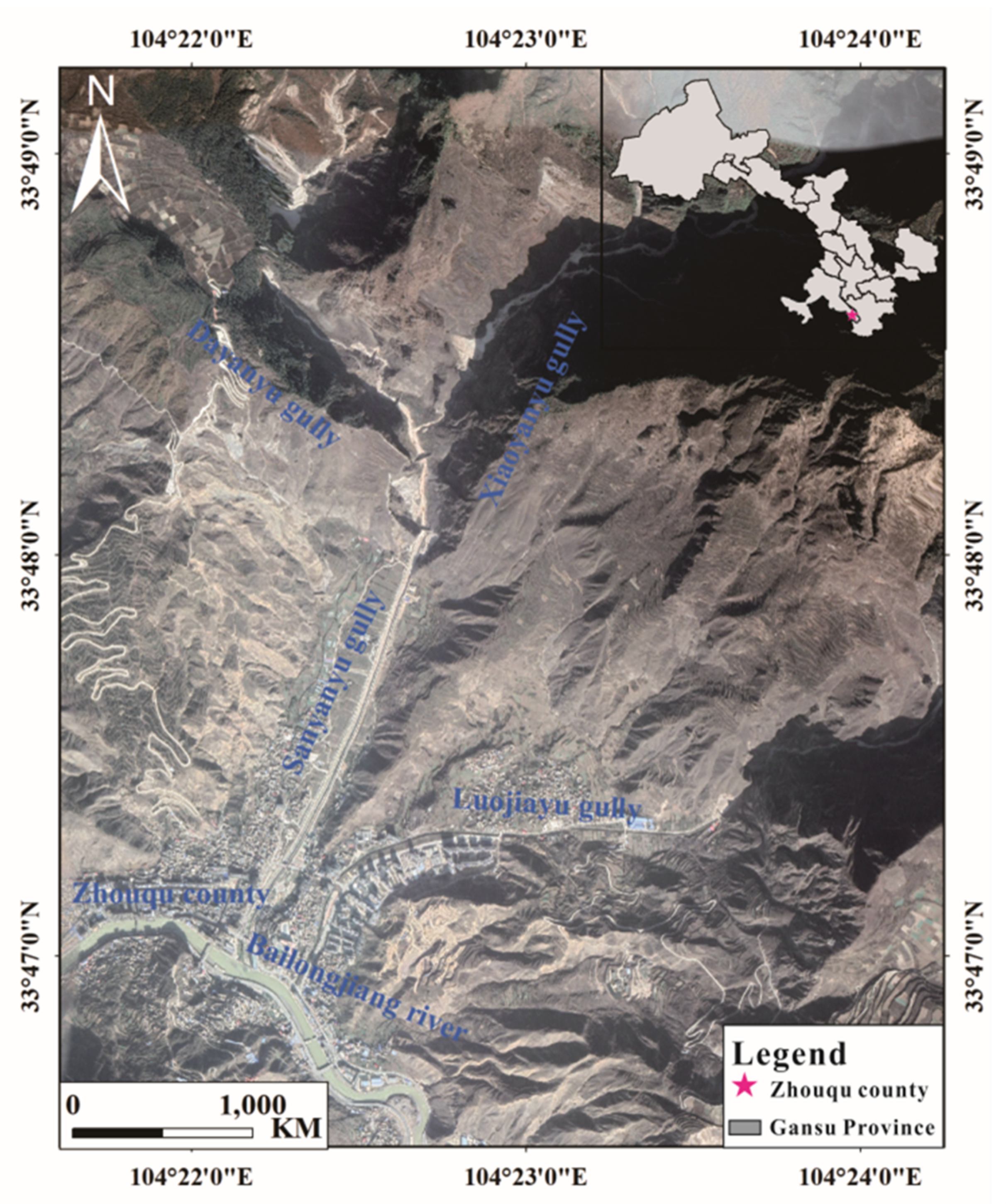
At approximately 22:00 on 7 August 2010, torrential rain suddenly occurred in the northern mountainous area of the eastern part of Zhouqu County, Gansu Province. Ninety-seven millimetres of rainfall were recorded during this event, which lasted for more than 40 min, resulting in catastrophic mountain torrents in four gullies, including the Sanyanyu gully and Luojiayu gully (Figure 1). The debris flow was approximately 5 km long, with an average width of 300 m, an average thickness of 5 m, and a total volume of 7.5 million cubic meters. More than 5000 houses and other infrastructure were impacted and buried. The solid materials blocked the Bailong River, a tributary of the Jialing River, and formed a barrier lake. Power, transportation, and communication in the region were completely interrupted. A total of 1557 people were killed and 284 people were missing in the Zhouqu debris flow, the most serious debris flow event in China [44,45].
The Sanyanyu gully watershed in Zhouqu County, Gansu Province is a tributary of the left bank of the Bailong River, with a drainage area of 25.75 km2. The gully is generally distributed from south to north, with high terrain from north to south and low terrain from south to north, which is typical alpine canyon topography. The highest point of the basin is 3828 m above sea level and the lowest point is only 1340 m above sea level at the estuary, with a relative elevation difference of 2488 m. According to statistics, there have been many large-scale debris flows in this area and the “8.7” Zhouqu debris flow is the most serious debris flow disaster in the history of this area [46,47].
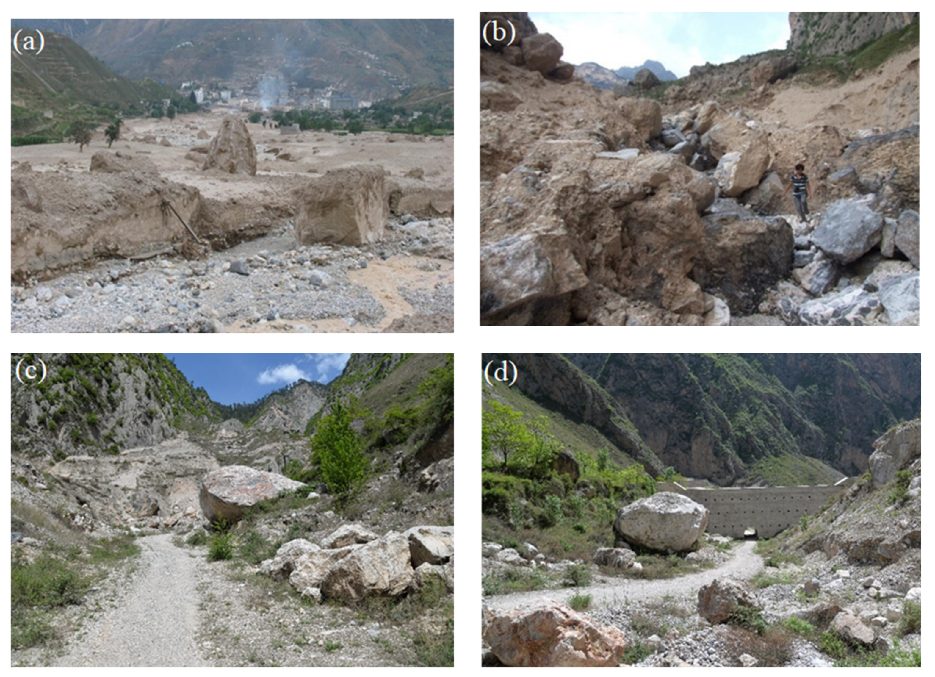
The Zhouqu debris flow caused the deposition of a large amount of material, and massive boulders mixed in the debris flow caused great damage to downstream buildings, prevention and control projects, and other infrastructure (Figure 2). Figure 2a shows a large number of huge boulders in the accumulation area, which pose a serious threat to the downstream buildings. The diameter of the boulder in Figure 2d is approximately 18 m; such a boulder could severely undermine the structural stability of the check dam in the event of a debris flow outbreak. At present, research on debris flow impact is mainly focused on debris flow slurry, and there is relatively little attention and research on the movement characteristics and impact of boulders submerged in debris flows.
3. Numerical Model of the Zhouqu Debris Flow
Owing to the limitations of traditional observation and theoretical methods, it is very difficult to study the movement characteristics of rocks submerged in debris flows. The numerical method can solve the nonlinear and complex fluid–solid coupling problem. To accurately predict the movement characteristics of boulders in the Zhouqu debris flow, the FLOW-3D software was applied to simulate the motion of boulders with different shapes under the action of the debris flow. The GMO and RNG turbulence models were used to present the boulders and debris flow, respectively. This model has been used to analyze the waves generated by landslides [40].
The RNG turbulence model was adopted to describe the movement of debris flow in Zhouqu County. This model can accurately simulate the movement characteristics of debris flow under the premise of a single-phase flow [48]. The two transport equations for the RNG model are as follows:
where kT is the turbulent kinetic energy, VF is the fractional volume open to flow, and Ax, Ay, and Az are the fractional area open to flow in the x-, y-, and z-directions, respectively. PT is the turbulent kinetic energy production term, GT is the buoyancy production term, Diff is the diffusion term, and εT is the turbulence dissipation term. CDIS1 = 1.42, CDIS2, and CDIS3 = 0.2 are dimensionless parameters. CDIS2 is computed from the turbulent kinetic energy (kT) and turbulent production (PT) terms [48].
A GMO is a rigid body. It can be either fully dynamically coupled with fluid flow or be user-prescribed. The moving object can move with six degrees of freedom or rotate about a fixed point or a fixed axis. The GMO model allows users to simulate the motion of multiple moving objects simultaneously. Meanwhile, this model allows the user to define the rebound effect using the coefficient of restitution and coefficient of friction. The motion parameters of each object can be conveniently obtained.
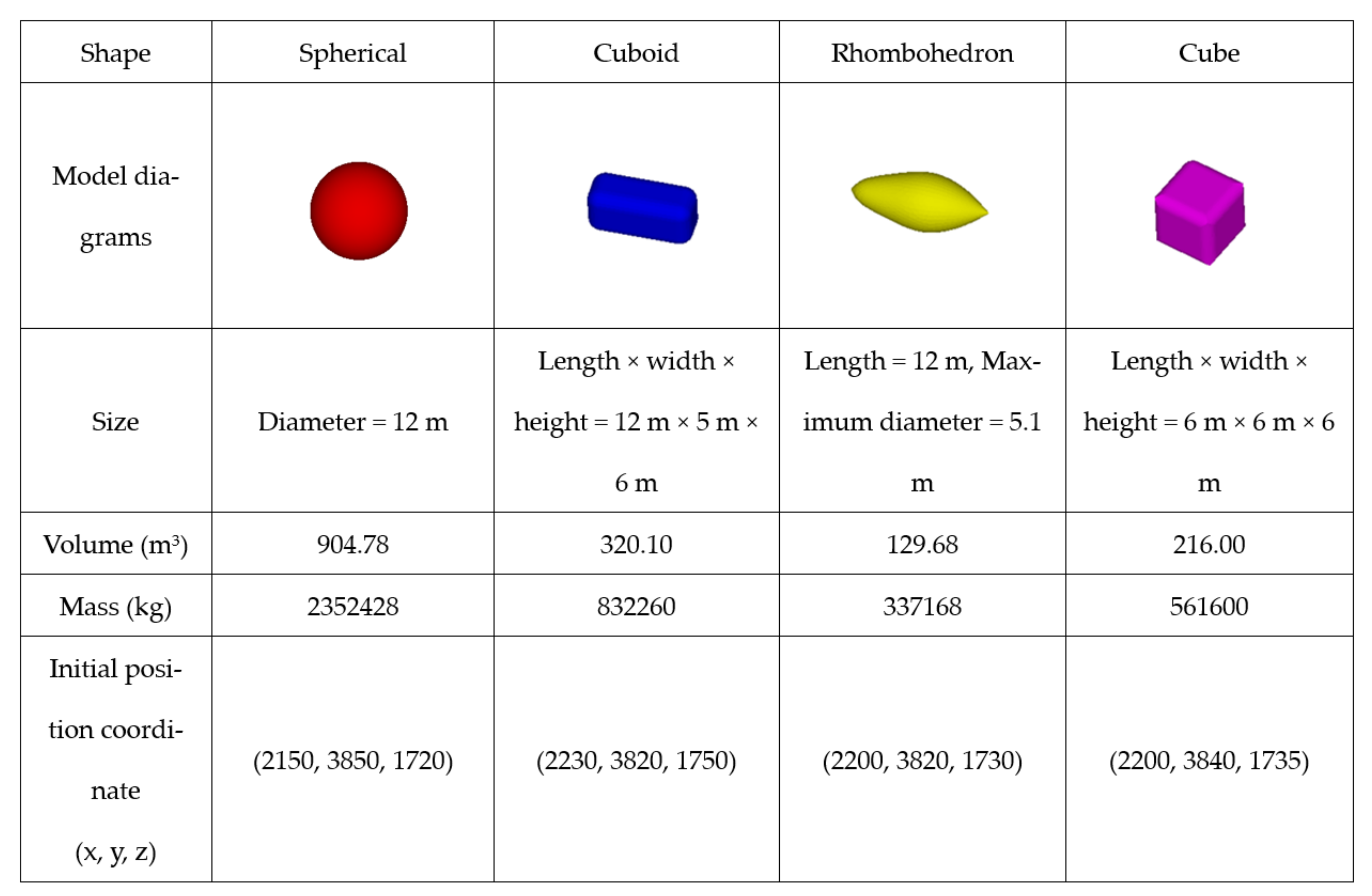
Although the boulders are large in volume, they are relatively small in number and are often buried by the soil. In the field survey before the occurrence of debris flow, the boulders are not considered as an investigation item of debris flow source. At present, the study on the size and shape of boulders carried by the debris flow is only after the occurrence of debris flow, so the initial location and volume of boulders cannot be determined. In this study, four different shapes of boulders were defined in the GMO model. According to the results of the field investigation by Hu et al. [19], spherical, cuboid, rhombohedral, and cube-shaped boulders were adopted in the simulation. However, the initial positions were set by the authors to study the influence of the boulder shape on their movement characteristics. The boulder models were first established in AutoCAD software. Next, the STL file was exported and then imported into FLOW-3D software. The density of boulders was 2600 kg/m3 according to the field survey data. Owing to the large mass of the boulders, the restitution coefficients (e) and the friction coefficient (μ) used in the simulation are 0.10 and 0.35, respectively. The restitution coefficients (e) are the square root of the ratio of h2 to h1 (h1 is the height before the rebound, h2 is the height after the rebound), which is between 0 and 1. Due to the large mass of the boulders and the soft ground with water on its surface, we believe that the boulders basically have no rebound; therefore, this value is empirically obtained as 0.10. The friction coefficient (μ) is the ratio of the tangential force to the normal stress on the contact surface. Because there is no relevant research on this parameter, we used the friction coefficient of hard clay against the base of the retaining wall to approximate this coefficient. This value can be found in Table 6.6.5-2 of P44 of the National standard of the People’s Republic of China, Code for Design of Building Foundation [49]. The specific information of these boulders is shown in Figure 3.
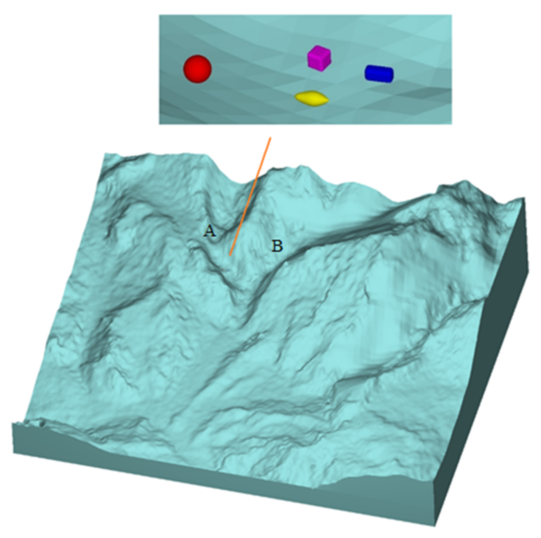
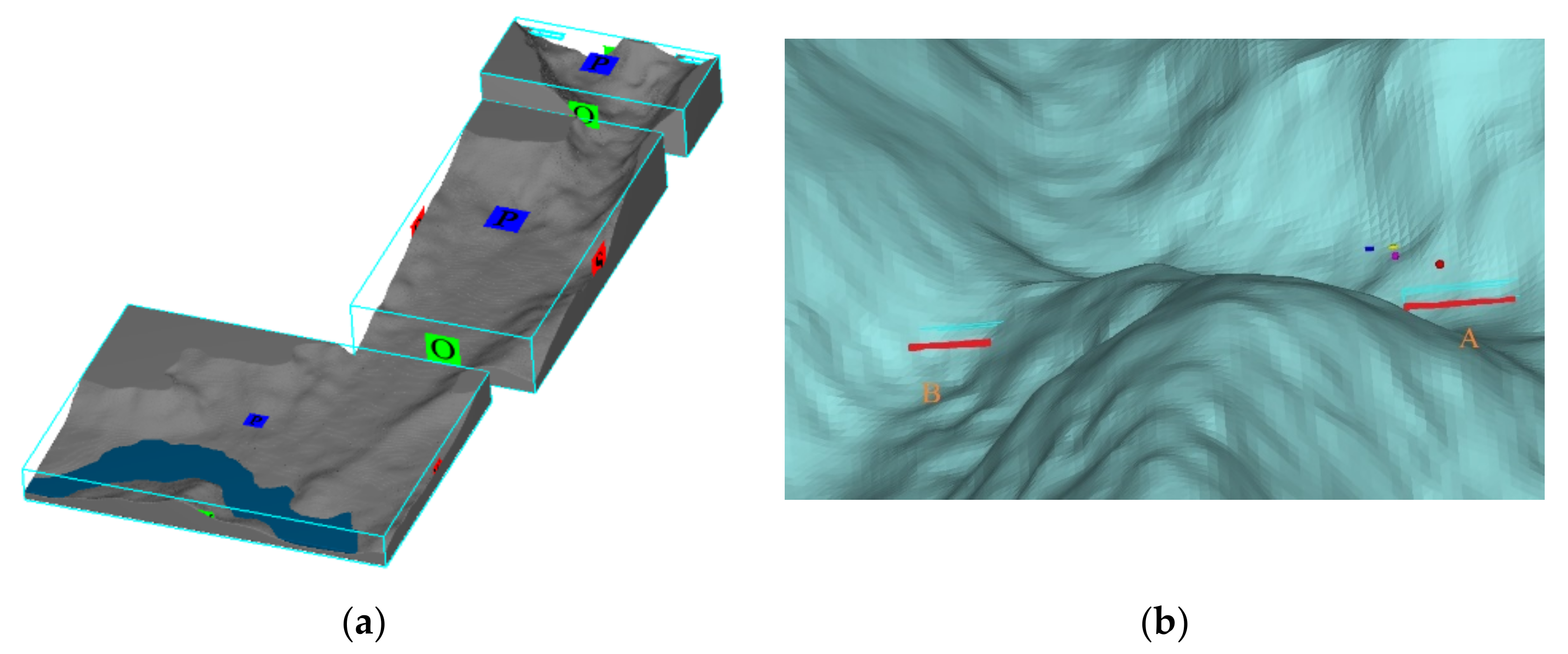
The topographic map of the Zhouqu debris flow is based on digital elevation model (DEM) data, with a length of 6.412 km and a width of 5.25 km. The DEM terrain range and initial position of the boulders and debris flow boundary entrance (section A and B) are shown in Figure 4 and Figure 5b. There are four boulders in each simulation, and they are placed almost at the same position. The arrangement of the boulders is random, but the arrangement is the same in each simulation condition. Since the boulders travel relatively long distances, their initial arrangement is not very important in this simulation. However, it is necessary to make them basically at the same starting position, so as to better simulate the influence of the boulder shape on their motion characteristics. Owing to limited computer memory resources, five mesh blocks were used to divide the study area and the mesh cells in the simulation were 21,984,310 in total. The boulders moved from the initial position to the Bailong River and then stopped. The total calculation time was 220 s. Figure 5a,b show the meshing range of the simulation and the schematic diagram of rectangular debris flow inlet (section A and B), as shown in the red area in Figure 5b.
In the process of transportation of a natural debris flow, the density changes with the change in flow discharge, and its properties also change constantly. For various types of debris flows, different mathematical models are needed; the Bingham fluid, dilatant fluid, viscoplastic fluid, and Coulomb mixture models are usually used to describe the debris flow [50,51]. In this simulation, the Bingham debris flow model was selected, as shown in Equation (3).
where τ is the shear stress, τy is the yield stress, η is the viscosity coefficient, and du/dy is the flow velocity gradient. According to the quantitative relationship between the yield stress and density for Jiangjia gully debris flows (Equation (4)) [52], as well as that between the stiffness coefficient and the yield stress for a debris flow density larger than 1300 kg/m3 (Equation (5)) [53], the following equations were used:
where τy is the yield stress, ρ is the debris flow density, and η is the viscosity coefficient. According to Equations (4) and (5), the simulation parameters of debris flow densities of 1200 kg/m3, 1500 kg/m3, 1800 kg/m3, and 2100 kg/m3 can be calculated, as shown in Table 1.
The initial boundary conditions of debris flow are determined according to the post-disaster field investigation results of Zhouqu debris flow by Hu et al. [54], and the specific parameters are shown in Table 2. The debris flow depth and velocity at the rectangular inlets (Figure 5b) remain constant throughout the simulation.
4. Results of the Simulation
4.1. Movement Process of the Boulders
Figure 6a shows the movement process of four types of boulders under the action of a debris flow with a density of 2100 kg/m3. In the simulation, the boulders are mainly arranged in the Dayanyu gully, the movement progress of which can be divided into two stages according to the obvious change in the terrain slope. In the first stage, the boulder moves in the circulation area where the Dayanyu gully and Xiaoyanyu gully intersect. In this stage, the terrain slope is relatively large, and the average gradient of the gully reaches 12%. In the second stage, the movement is in the accumulation area from the Sanyanyu gully to the Bailongjiang River and the terrain slope is relatively gentle with an average gradient of 9%. The obvious change in terrain slope in these two stages will have a great impact on the movement of boulders. In the simulation (Figure 6a), the debris flows in the Dayanyu gully and Xiaoyanyu gully began to converge after 30 s. When the simulation time was 90 s, the debris flow moved in the Sanyanyu gully with a gentle slope. When the simulation time was 180 s, the debris flow moved into the Bailongjiang River. According to the simulation, the surface velocity of the debris flow reached its maximum of approximately 30 m/s downstream of the intersection. After that, the flow velocity gradually decreased to 18 m/s. The boulders moved along the gully under the action of debris flow. At 30 s, the direction of the boulder movement began to turn due to the influence of terrain and moved downstream along the Sanyanyu gully and some boulders rolled into the Bailong River. By observing boulder movement under other simulation conditions, it can be seen that boulder movement is not only affected by the size, shape, and mass of the boulder, but also by topographic factors, the coupling effect of debris flow, and the collision of boulders in the movement process. Therefore, it is necessary to analyze the laws of the movement and accumulation of boulders from the changes in their motion parameters. Figure 6b show the snapshots of cube and spherical boulders flowing into the river for a debris flow of 2100 kg/m3.
4.2. Velocity Variation Characteristics of Boulders
4.2.1. Influence of Density
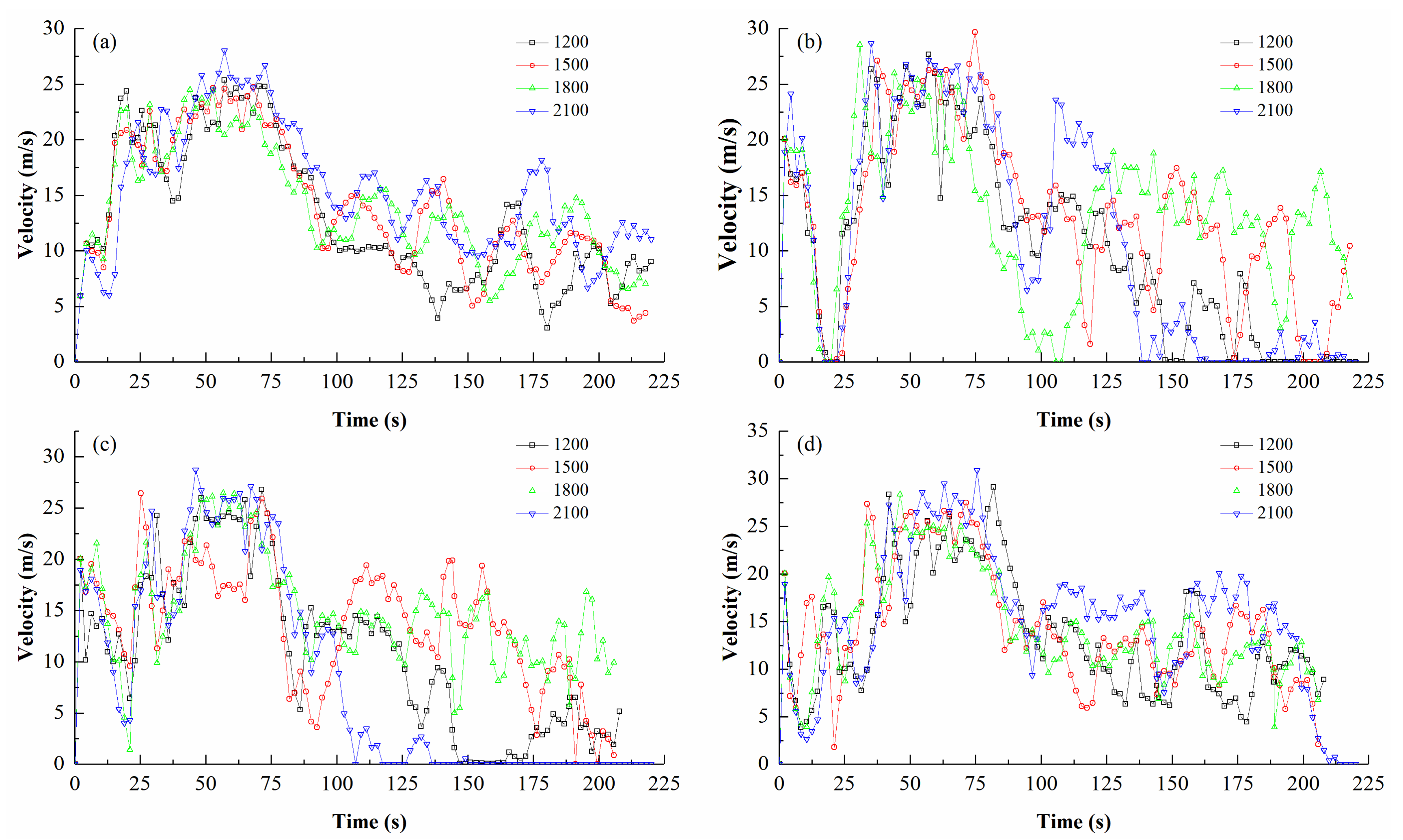
Figure 7 shows the changes in the centroid velocity of the boulders with debris flow densities of 1200 kg/m3, 1500 kg/m3, 1800 kg/m3, and 2100 kg/m3. It can be seen from Figure 7 that the velocity of the four shapes of boulders increases first and then decreases gradually, which is consistent with the change in terrain slope. At T = 75 s, the slope of the terrain gradually decreased, and the average velocity of the boulders gradually slowed to approximately 13 m/s (Figure 7a). In this stage, the motion velocity of the spherical boulder is essentially positively correlated with the increase in the debris flow density and the variation amplitude of the velocity is relatively small, whereas the motion velocity of other shaped boulders has little correlation with the debris flow density. Similar conclusions can be preliminarily seen from our previous research, that is, the motion velocity of spherical boulders is positively correlated with the density of debris flow [55]. In this study, the velocity of the spherical boulders is not only affected by debris flow density, but also by the irregular slope of natural terrain. Therefore, this correlation was not always valid in this study and we cannot give a specific correlation formula between them.
4.2.2. Influence of Shape
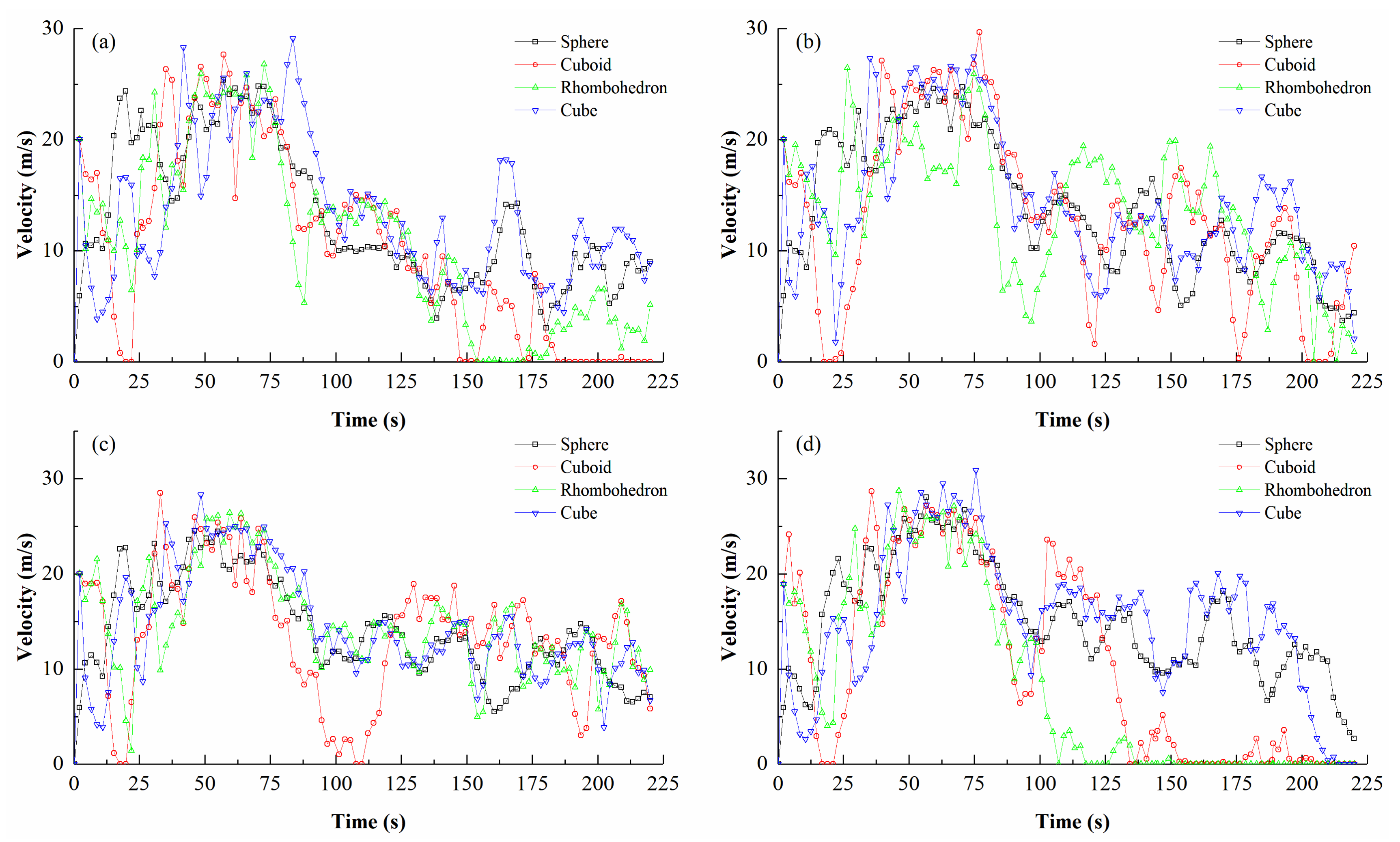
Figure 8 shows the changes in the centroid velocity of the four kinds of boulders with a specific debris flow density. As the movement of boulders is affected by a variety of factors and has complex three-dimensional characteristics, it is difficult to identify the change rule that is influenced by shape. Under the simulation condition of debris flow densities of 1200 kg/m3 and 2100 kg/m3, the velocity of cuboid and rhombohedron boulders reaches zero and stops first compared with the spherical and cube boulders (Figure 8a,b). This may be related to the inconsistency of the edge length of cuboid and rhombohedron boulders, which makes it difficult for them to move along a straight line. The spherical and cube boulders have a symmetrical appearance and can move longer distances under the same conditions.
4.3. Angular Velocity Variation Characteristics of Boulders
4.3.1. Influence of Density
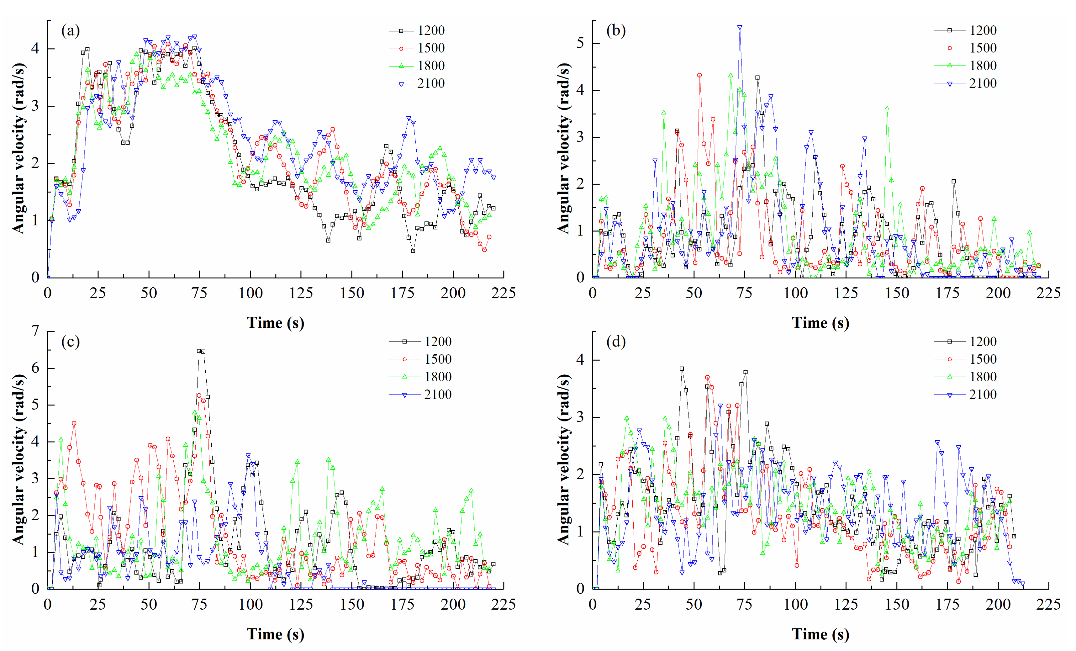
Figure 9 shows the variation in the angular velocity of the boulders with time under the condition of density change. It can be seen from the curves in Figure 9 that the angular velocity of spherical boulders has a small fluctuation amplitude with time, whereas the angular velocity of cuboid, rhombohedron, and cube boulders presents a peak pattern of “increasing-decreasing” throughout the movement process. This is mainly because under the action of debris flow, when the centre of gravity of the cuboid, rhombohedron, and cube boulders passes over the bottom edge, it decreases under the action of gravity, and the angular velocities first increase and then decrease rapidly when it touches the ground. However, the height of the centre of gravity from the ground for the spherical boulder did not change during the movement. Therefore, the curves of the angular velocity of the spherical boulder will not present a “peak.” When the terrain slope is large (T = 0–75 s), the angular velocity of the sphere increases rapidly, whereas the increase of angular velocity for the cuboid, rhombohedron, and cube boulders is relatively small (Figure 9b–d). This is because the edges and corners of the boulders hinder its rolling, making the boulder move in a rolling and sliding manner. When the terrain slope is less (T = 75–220 s), the angular velocity of spherical boulders increases with the increase in flow density, but it is difficult to observe this phenomenon for other boulders with edges and corners, which is mainly related to the shape of the boulders.
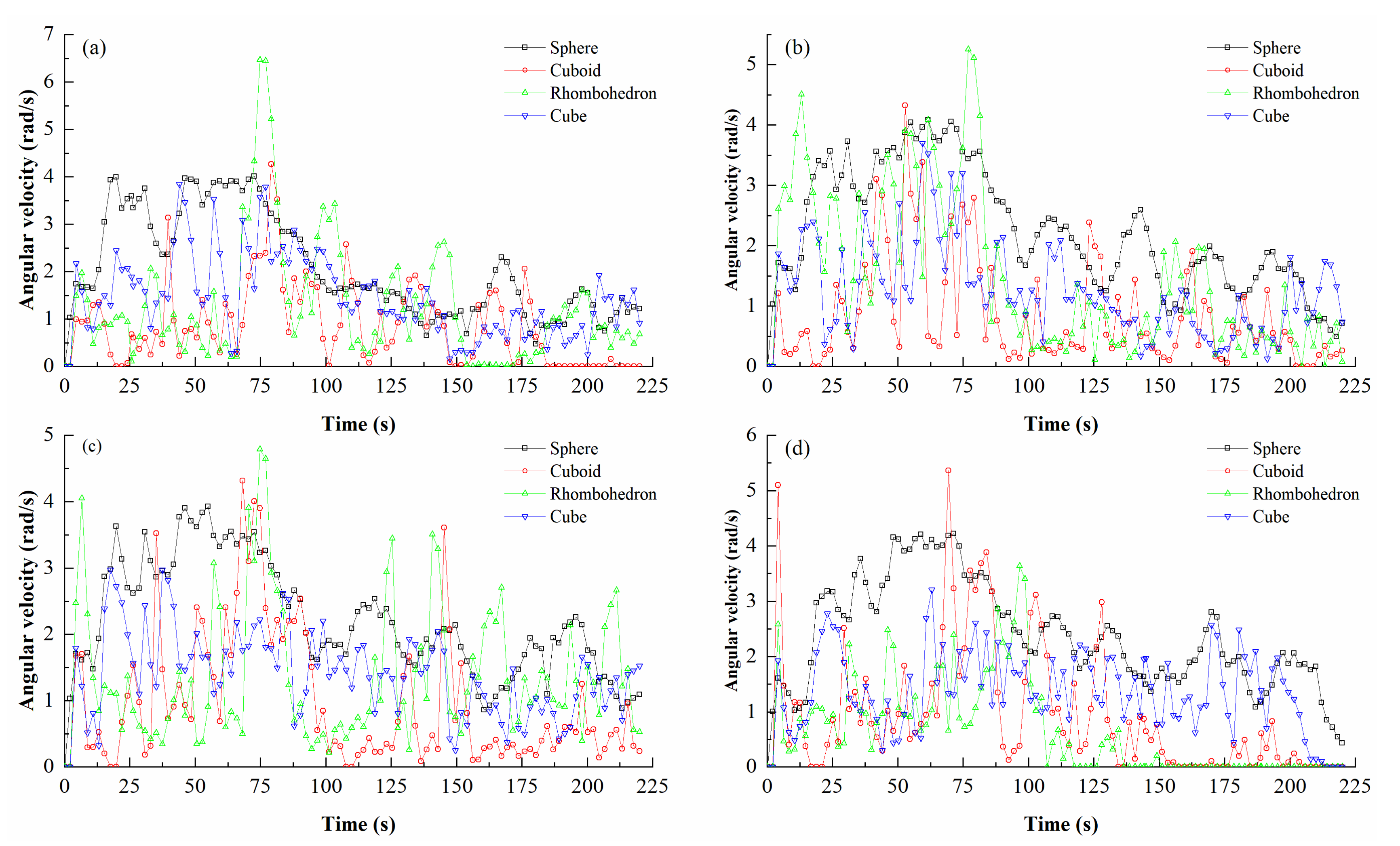
4.3.2. Influence of Shape
Figure 10 shows the angular velocity curves of different shapes of boulders under the conditions of debris flow density of 1200 kg/m3, 1500 kg/m3, 1800 kg/m3, and 2100 kg/m3. It can be seen from the figures that the angular velocity of spherical and cube boulders is greater than that of boulders of other shapes most of the time under four kinds of flow densities, with the angular velocity of the cuboid boulder being the smallest. This is because the shape of the boulder with spherical symmetry and the smoothness of its surface has an important influence on its angular velocity. The spherical boulder not only has a spherically symmetrical shape but also has a smooth surface; therefore, the angular velocity is the largest. Although the axis of symmetry of the cube boulder is the same in length and approximately spherically symmetric, the surface is not smooth enough. The length of the symmetry axis of rhombohedron boulder is different but the surface is smooth. However, the length of the symmetry axis of a cuboid boulder is not the same and the surface is not smooth. Therefore, most of the time, the angular velocity of the cuboid boulder is the least.
4.4. Kinetic Energy Variation Characteristics of Boulders
Boulders roll forward under the action of debris flow slurry. They have a very large kinetic energy and pose a great threat to buildings. According to the above analysis, the kinetic energy of the boulders mainly includes two aspects, namely the translational kinetic energy and the rotational kinetic energy of the boulder, as shown in Equation (6):
where m is the mass of the rigid boulders, v is the velocity of the centre of mass, Ic is the rotational inertia of the rigid body to the centroid axis, and ω is the angular velocity of the rigid boulders.
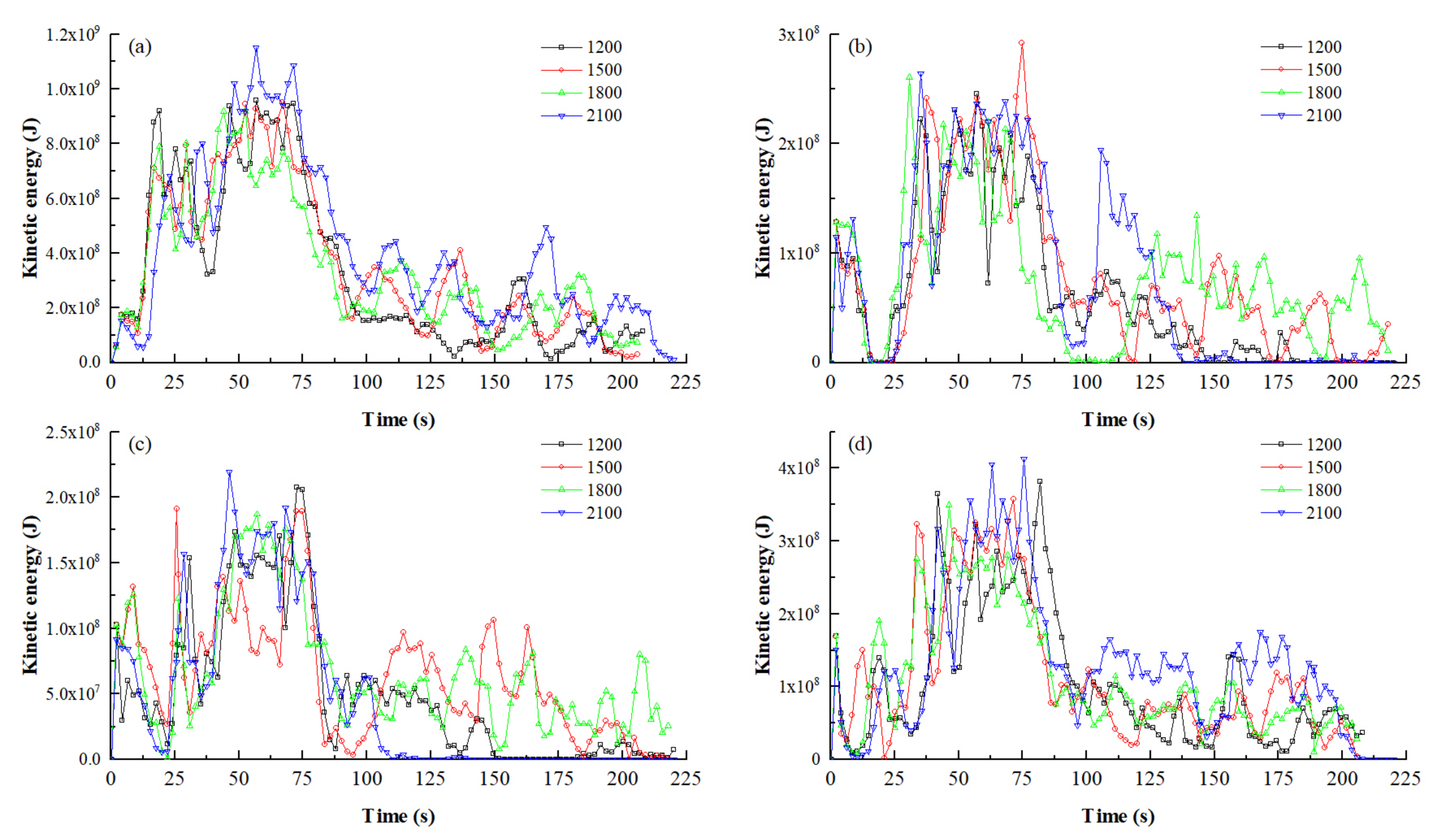
4.4.1. Influence of Density
Figure 11 shows the kinetic energy curve of the four kinds of boulders under different flow density conditions. The change curve of boulder kinetic energy is very similar to that of the centroid velocity of boulders. This indicates that the translational kinetic energy of boulder motion accounts for most of the total kinetic energy.
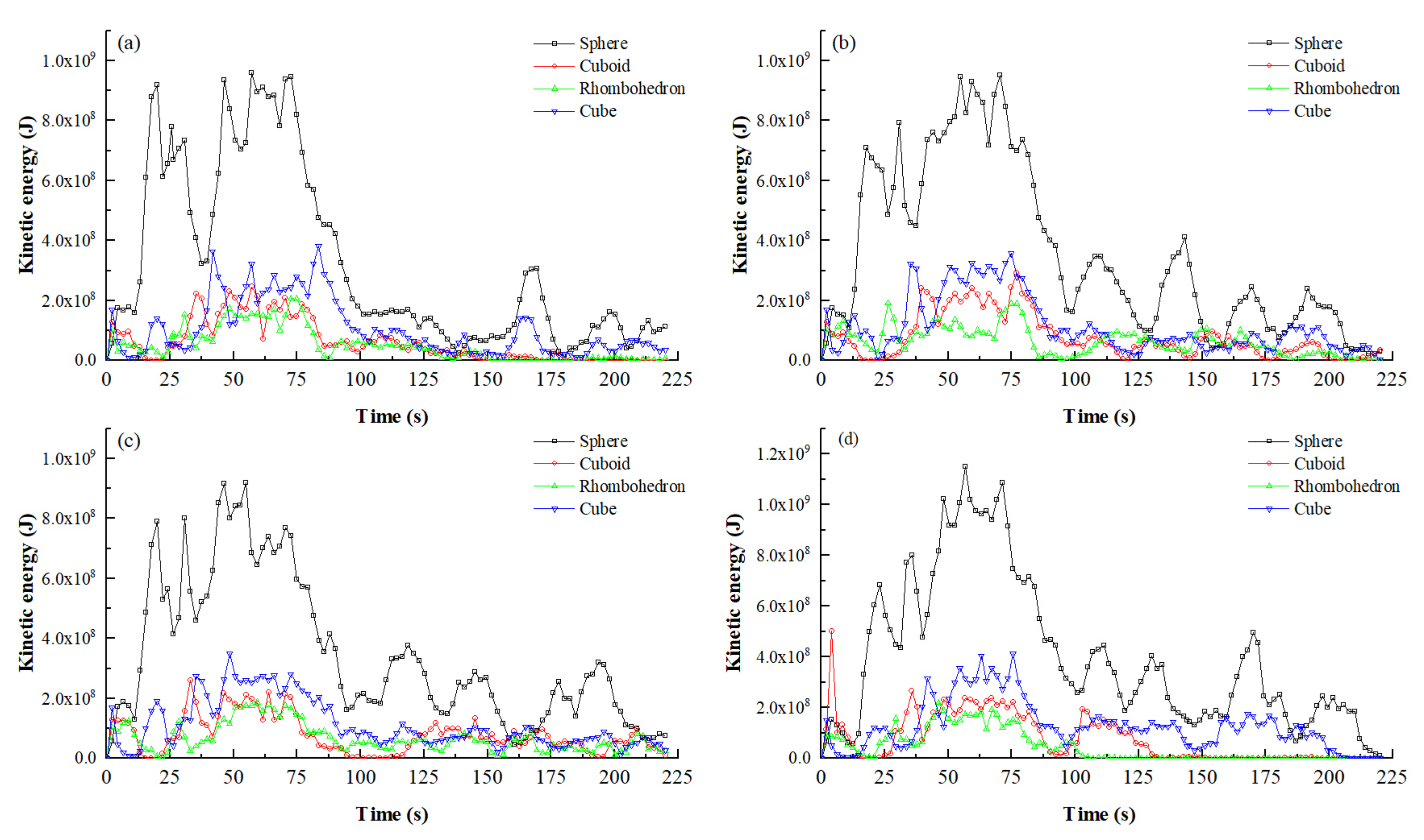
4.4.2. Influence of Shape
Figure 12 shows the kinetic energy of different shapes of boulders under debris flow density of 1200 kg/m3, 1500 kg/m3, 1800 kg/m3, and 2100 kg/m3. It can be seen from the figures that the kinetic energy of the sphere is far greater than that of other shapes of boulders, which is related to its larger mass. In addition, the kinetic energy also decreases after the slope becomes gentle, which indicates that the terrain slope has a great influence on the velocity and kinetic energy of boulders. Therefore, corresponding engineering measures can be adopted to reduce the energy of boulders in the debris flow, such as the use of check dams to block the boulders in the channel or the installation of concrete retaining walls and deceleration baffles in front of buildings to absorb the energy [56].
5. Discussion
5.1. Boulder Movement Range
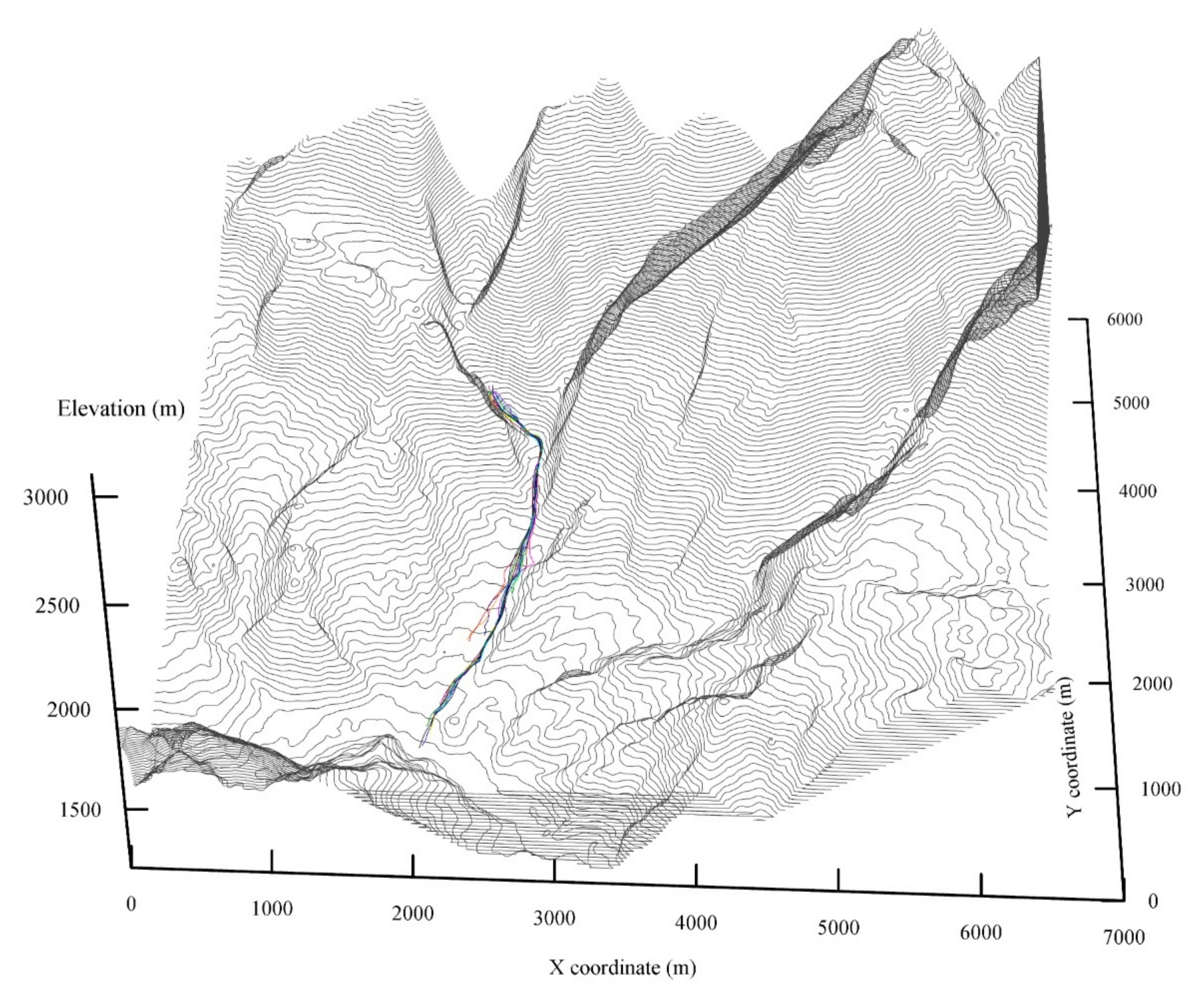
Owing to the potential danger of boulders submerged in debris flows, the possible threat range of boulder movement can be obtained through multiple simulation calculations of boulder movement. According to the above research on the velocity, angular velocity, and kinetic energy of boulders, the movement of boulders in debris flows is affected by many factors, and it is very difficult to determine the movement parameters of boulders. Therefore, multiple simulation methods can be used to obtain the range of motion parameters, such as the upper limit of the centroid velocity (Figure 7 and Figure 8), which can provide effective parameters for the design of debris flow engineering measures. In addition, the possible threat range of boulder movement can be obtained based on multiple simulations, as shown in Figure 13, which can provide references for the long-term planning of infrastructure such as houses, schools, and factories.
5.2. Boulder Movement Distance
5.2.1. Influence of Density
The change curves of the movement distance of the boulders under different density conditions can be obtained by calculating the movement distance between two adjacent time intervals according to Equations (7) and (8):
where Dn is the distance between the nth point and the n-1th point, Xn, Yn, and Zn are the spatial coordinates of the nth point, and Sn is the total distance from the nth point to the initial position.
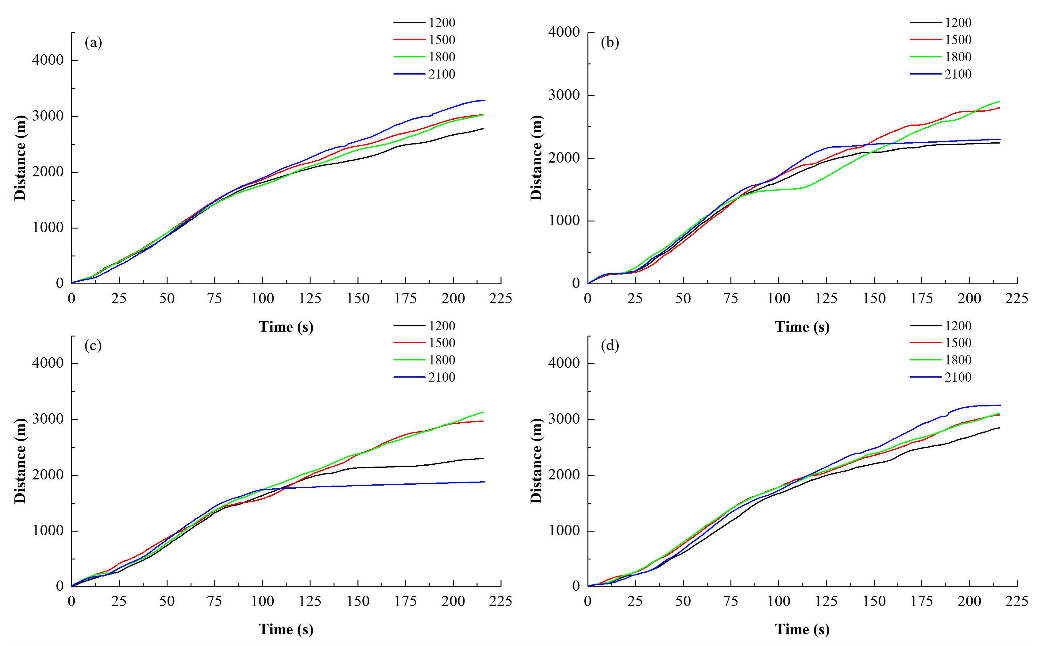
It can be seen from Figure 14 that when the terrain slope is large (T = 0–75 s), the movement distance curves almost overlap, indicating that the debris flow density has a relatively small influence on the movement distance for different boulder shapes. However, when the terrain gradient becomes gentle (T = 75–225 s), the movement distance curves of different shapes of boulders gradually separate, and the value of some curves stops changing, indicating that the boulders stop moving. This phenomenon implies that when the slope is large, the appearance characteristics of the boulders have less influence on the movement distance and when the slope is less, the influence of the appearance characteristics of the boulders is greater. This is because when the slope is large, the gravity component of the boulder can be greater than the resistance of the boulder’s appearance, and when the slope is less, the dynamics of the boulder’s movement are insufficient, and the resistance brought by its appearance and shape will cause it to stop moving.
It can also be seen from Figure 14 that the greater the density of debris flow, the farther the spherical and cubic boulders travel (Figure 14a–d); however, the moving distance of rhombohedron and cuboid boulders may be closer (Figure 14b,c). We believe that the shapes of the spherical and cube shaped boulders are basically symmetrical and can maintain the same flow direction as the debris flow. The greater flow density will cause them to move further. However, the movement direction of the cuboid and rhombohedron boulders and the flow direction of debris flow cannot be completely maintained due to their appearance characteristics. The greater density of debris flow can cause them to move at a faster velocity, potentially pushing out of the fluid range of the debris flow and stopping moving.
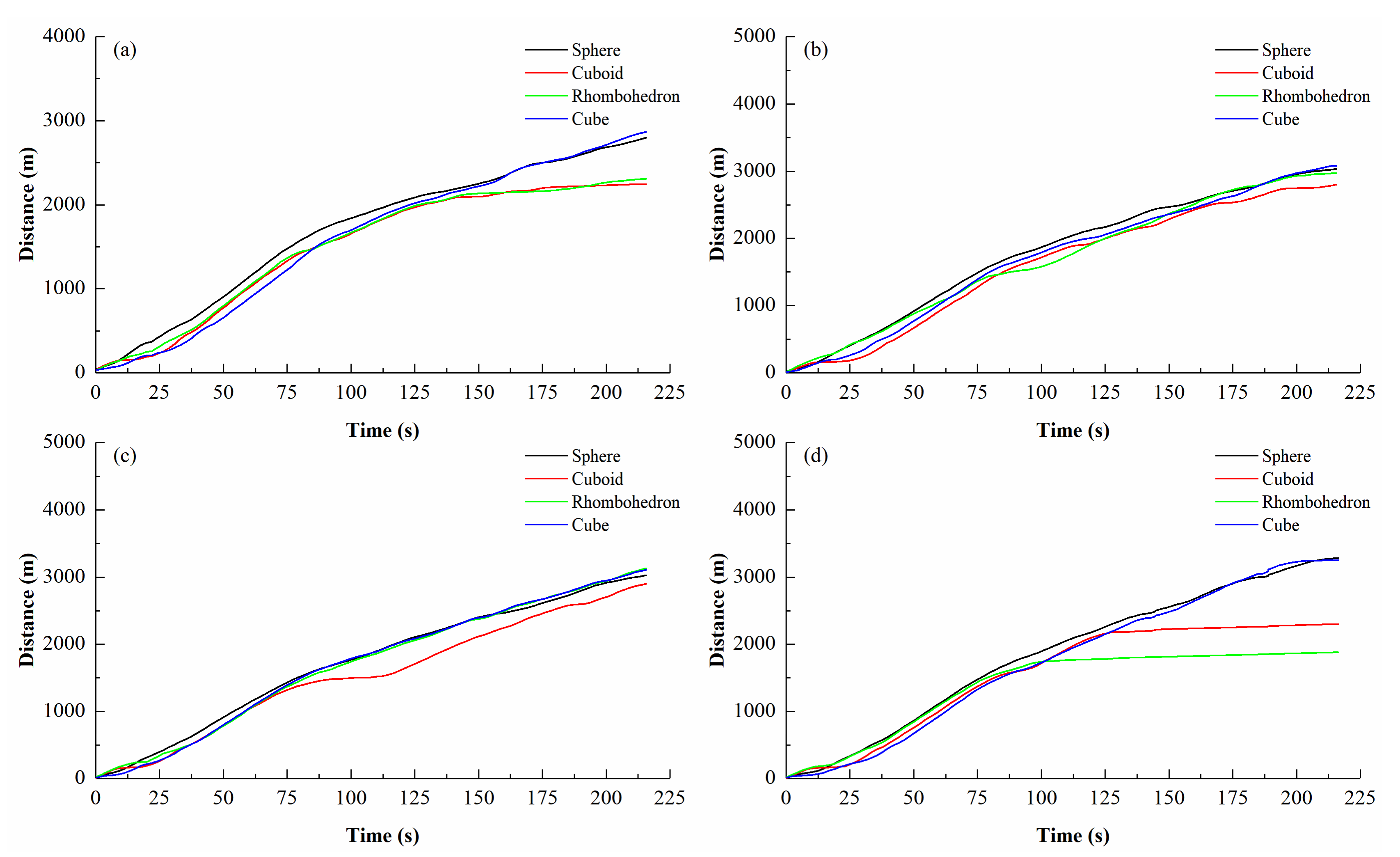
5.2.2. Influence of Shape
Figure 15 shows the variation curves of the movement distance of boulders with different shapes under the conditions of debris flow density of 1200 kg/m3, 1500 kg/m3, 1800 kg/m3, and 2100 kg/m3. From Figure 15, it can be seen that the spherical and cube boulders have a longer movement distance, whereas the cuboid and rhombohedron boulders have lesser movement distance and some of them will stay in the accumulation area. This is because the closer the boulder shape is to the spherical symmetry, the smoother the surface is, and the greater the cumulative movement distance is. In the movement process, a boulder with a non-spherical shape may not be able to move in a straight line due to its appearance. Instead, it may move to one side of the gully, out of the range of the debris flow, and may stop due to lack of dynamics. On the other hand, the gravity center of the cuboid and rhombohedron boulders will fluctuate up and down during the rolling movement, while the height of the gravity center of the spherical boulder will remain unchanged during the movement. Therefore, a part of the kinetic obtained from the debris flow of the cuboid and rhombohedron boulders used to overcome the acting of its gravity, thus reducing the kinetic energy obtained in the horizontal direction. This is also an important reason for their small moving distance [31,57]. These simulation results are essentially consistent with the field research of Hu et al. [19] that most of the boulders in the accumulation area are cuboid and rhombohedron boulders.
5.3. Dynamic Impact Force of the Boulders
The impact force of debris flow can be divided into two kinds: one is the dynamic pressure load of debris flow fluid, the other is the impact force load of the boulders in the debris flow slurry. The dynamic pressure load of debris flow fluid was initially based on the one-dimensional static fluid model [58], and then some empirical models suitable for different conditions were developed on this basis [59]. The calculation of the impact force of boulders in debris flow includes the theoretical model of elastic spherical impact force, the calculation formula of the impact force of plastic plane and rigid sphere, and the calculation formulas of cantilever beam and simply supported beam impacted by boulders [60]. In addition, the impact force of debris flow slurry and boulders can be obtained through the numerical simulation [61,62,63]. The difficulty in calculating the impact force of boulders in debris flow is to determine the movement velocity of boulders under the influence of multiple factors and calculate the impact duration of interaction with infrastructures. The simulation method adopted in this study can obtain the velocity variation process well under the coupling of boulder and debris flow slurry, which can provide reference for engineering prevention and control. According to the momentum theorem Ft = mv2 − mv1, the collision force between a boulder and a structure is inversely proportional to its collision time. We assume that the velocity of the boulder is zero after the collision, and compare the impact force of the rhombohedron boulder when the three collision durations are 0.1 s, 0.3 s, and 0.6 s. The simulation results show that the velocity of rhombohedron boulder is 14.64 m/s when t = 150 s under the action of debris flow with a density of 1800 kg/m3. It can be calculated that the impact force of the rhombohedron boulder on a structure is 4.94 × 10⁷ N, 1.65 × 10⁷ N, and 0.82 × 10⁷ N when the interaction time is 0.1 s, 0.3 s, and 0.6 s, respectively. The impact force of the rhombohedron boulder can reach six times when the action time is reduced from 0.6 s to 0.1 s. Therefore, reducing the rigid collision between boulders and buildings can effectively reduce the impact force on infrastructures from the perspective of engineering protection. In engineering practice, decelerating obstacles such as waste tires, mounds, or concrete piers can be arranged in front of the protected objects to absorb the impact of boulders.
5.4. Limitation of the Study
Through the above simulations, it can be seen that the fluid–solid coupling model applied in this study can be used to obtain the movement parameters of boulders submerged in debris flows. The research results can reveal the movement mechanism of boulders in debris flows and provide a reference for engineering design. However, due to time constraints, resources, and other aspects, this study has some limitations, including the following: (1) although this study is based on the Zhouqu debris flow, the scanning model of the on-site boulders is not adopted for certain reasons; thus, the boulder model adopted in the simulation is somewhat different from reality; moreover, there is no observation data on the movement of boulders in debris flows; therefore, the simulation results cannot be directly verified; (2) the topographic map data of the Zhouqu County area used in the simulation are not accurate enough, which may affect the simulation results; (3) limited computing resources led to a certain difference between the boulder model and the imported STL file after meshing, which will have a certain influence on the calculation results; (4) mesh sensitivity studies will be conducted in the future to ensure that the results do not depend on discretization, so as to improve the reliability and computational efficiency of numerical results. In the follow-up research, we will solve the above problems to make the simulation results closer to the real situations.
6. Conclusions
Based on the results of relevant references and numerical simulation analysis on the motion characteristics of boulders with different shapes that interact with debris flow in Zhouqu County, the following conclusions can be drawn:
- (1)
- The motion characteristics of boulders in the 8.7 Zhouqu debris flow were simulated using FLOW-3D software with the GMO and RNG coupled models. The simulation results can be used to obtain various motion parameters of the boulders that interact with the debris flow slurry, such as the centroid velocity, angular velocity, kinetic energy, and motion trajectory. This method has a certain reference for studying the movement mechanism of debris flow.
- (2)
- The simulation results show that the movement velocity of boulders is affected by many factors such as terrain conditions, debris flow densities, and shapes of the boulders. When the terrain slope is relatively large, the boulders have greater potential energy, and the influence of terrain on the movement velocity of boulders is greater than that of debris flow density and boulder shape. When the slope is less, the appearance of boulders has a great influence on its movement. The velocity of a spherical boulder increases with debris flow density. However, the movement of cuboid, rhombohedron, and cube boulders presents a complex motion state, and it is difficult to predict the change law of their velocity.
- (3)
- The simulation results show that the angular velocity of the spherical boulder fluctuates slightly with time during the whole movement progress, whereas the angular velocity of the cuboid, rhombohedron, and cube boulders fluctuates continuously during the movement, presenting a peak form of “increasing-decreasing.” In addition, in most cases, the angular velocity of the spherical and cube boulders is larger than that of the cuboid and rhombohedron boulders. This indicates that the angular velocity variation law of boulder motion is related to whether the shape of the boulder is spherically symmetric, as well as the smoothness of the surface.
- (4)
- The simulation results show that motion distance is greatly influenced by the terrain slope and shape of the boulders. When the topographic slope is relatively large, the debris flow density and appearance characteristics of boulders have little influence. As the slope decreases, the boulders will gradually stop owing to insufficient dynamics. Moreover, the movement distance of the spherical and the approximately spherically symmetric cube boulders are greater than those of the cuboid and rhombohedron boulders. The accumulation characteristics of boulders in the simulation are generally consistent with the field investigation results.
- (5)
- Although the results of this study have simulated the coupled motion of debris flow and boulders under the influence of multiple factors, there are still some deficiencies in this study, such as the inaccuracy of the topographic map, limited computational resources, and boulder modeling. Further improvements can be made in subsequent studies.
Author Contributions
Conceptualization, F.W.; methodology, F.W.; software, S.Z.; validation, J.W. and X.C.; formal analysis, F.W.; investigation, H.Q.; resources, J.W. and X.C.; data curation, C.L.; writing—original draft preparation, F.W.; writing—review and editing, F.W.; visualization, C.L.; supervision, J.W. and X.C.; project administration, J.W.; funding acquisition, J.W. All authors have read and agreed to the published version of the manuscript.
Funding
This research was funded by The National Key Foundation for Exploring Scientific Instrument Program, grant number 42027806; The National Natural Science Foundation of China, grant number 41807252; The Second Tibetan Plateau Scientific Expedition and Research Program, grant number 2019QZKK0902; The Key Research and Development Program of Hebei Province, grant number 20375409D.
Institutional Review Board Statement
Not applicable.
Informed Consent Statement
Not applicable.
Data Availability Statement
The authors agree to make data supporting the results or analyses presented in this paper available upon reasonable request from the first author and corresponding author.
Acknowledgments
We are grateful for the support of the debris flow simulation test platform of the Department of Geology, Northwest University, China.
Conflicts of Interest
The authors declare no conflict of interest.
References
- Iverson, R.M. The physics of debris flows. Rev. Geophys. 1997, 35, 245–296. [Google Scholar] [CrossRef] [Green Version]
- Cui, P.; Chen, X.Q.; Zhu, Y.Y.; Su, F.H.; Wei, F.Q.; Han, Y.S.; Liu, H.J.; Zhuang, J.Q. The Wenchuan earthquake (May 12, 2008), Sichuan province, China, and resulting geohazards. Nat. Hazards. 2011, 56, 19–36. [Google Scholar] [CrossRef]
- Tang, C.; van Asch, T.; Chang, M.; Chen, G.; Zhao, X.; Huang, X. Catastrophic debris flows on 13 August 2010 in the Qingping area, southwestern China: The combined effects of a strong earthquake and subsequent rainstorms. Geomorphology 2012, 139–140, 559–576. [Google Scholar] [CrossRef]
- Cui, P.; Zhou, G.G.; Zhu, X.; Zhang, J. Scale amplification of natural debris flows caused by cascading landslide dam failures. Geomorphology 2013, 182, 173–189. [Google Scholar] [CrossRef]
- Chen, X.; Cui, P.; You, Y.; Chen, J.; Li, D. Engineering measures for debris flow hazard mitigation in the Wenchuan earthquake area. Eng. Geol. 2015, 194, 73–85. [Google Scholar] [CrossRef]
- Choi, S.-K.; Lee, J.-M.; Kwon, T.-H. Effect of slit-type barrier on characteristics of water-dominant debris flows: Small-scale physical modeling. Landslides 2018, 15, 111–122. [Google Scholar] [CrossRef]
- Wang, J.; Xu, Y.; Ma, Y.; Qiao, S.; Feng, K. Study on the deformation and failure modes of filling slope in loess filling engineering: A case study at a loess mountain airport. Landslides 2018, 15, 2423–2435. [Google Scholar] [CrossRef]
- Wang, J.; Zhang, D.; Wang, N.; Gu, T. Mechanisms of wetting-induced loess slope failures. Landslides 2019, 16, 937–953. [Google Scholar] [CrossRef]
- Qiu, H.; Zhu, Y.; Zhou, W.; Sun, H.; He, J.; Liu, Z. Influence of DEM resolution on landslide simulation performance based on the Scoops3D model. Geomat. Nat. Hazards Risk 2022, 13, 1663–1681. [Google Scholar] [CrossRef]
- Cui, Y.-F.; Zhou, X.-J.; Guo, C.-X. Experimental study on the moving characteristics of fine grains in wide grading unconsolidated soil under heavy rainfall. J. Mt. Sci. 2017, 14, 417–431. [Google Scholar] [CrossRef]
- Liu, D.; Cui, Y.; Guo, J.; Yu, Z.; Chan, D.; Lei, M. Investigating the effects of clay/sand content on depositional mechanisms of submarine debris flows through physical and numerical modeling. Landslides 2020, 17, 1863–1880. [Google Scholar] [CrossRef]
- Cui, P.; Zeng, C.; Lei, Y. Experimental analysis on the impact pressure of viscous debris flow. Earth Surf. Process. Landf. 2015, 12, 1644–1655. [Google Scholar] [CrossRef] [Green Version]
- Armanini, A. On the Dynamic Impact of Debris Flows. In Recent Developments on Debris Flows; Lecture Notes in Earth Sciences; Armanini, A., Michiue, M., Eds.; Springer: Berlin, Heidelberg, 1997; Volume 64, pp. 208–226. [Google Scholar]
- Liu, Z.; Qiu, H.; Zhu, Y.; Liu, Y.; Yang, D.; Ma, S.; Zhang, J.; Wang, Y.; Wang, L.; Tang, B. Efficient Identification and Monitoring of Landslides by Time-Series InSAR Combining Single- and Multi-Look Phases. Remote. Sens. 2022, 14, 1026. [Google Scholar] [CrossRef]
- Bugnion, L.; McArdell, B.W.; Bartelt, P.; Wendeler, C. Measurements of hillslope debris flow impact pressure on obstacles. Landslides 2012, 2, 179–187. [Google Scholar] [CrossRef] [Green Version]
- Choi, C.; Ng, C.; Song, D.; Kwan, J.; Shiu, H.; Ho, K.; Koo, R. Flume investigation of landslide debris–resisting baffles. Can. Geotech. J. 2014, 5, 658–662. [Google Scholar] [CrossRef]
- He, S.M.; Liu, W.; Li, X.P. Prediction of impact pressure of debris flows based on distribution and size of particles. Environ. Earth Sci. 2016, 4, 298. [Google Scholar] [CrossRef]
- Wang, D.; Chen, Z.; He, S.; Liu, Y.; Tang, H. Measuring and estimating the impact pressure of debris flows on bridge piers based on large-scale laboratory experiments. Landslides 2018, 15, 1331–1345. [Google Scholar] [CrossRef]
- Hu, G.S.; Chen, N.S.; Deng, M.F.; Lu, Y. Analysis of the Characteristics of Impact Force of Massive Stones of the Sanyanyu Debris Flow Gully in Zhouqu, Gansu Province. Earth Env. 2011, 4, 478–484. (In Chinese) [Google Scholar]
- Tan, D.-Y.; Yin, J.-H.; Feng, W.-Q.; Qin, J.-Q.; Zhu, Z.-H. New simple method for measuring impact force on a flexible barrier from rockfall and debris flow based on large-scale flume tests. Eng. Geol. 2020, 279, 105881. [Google Scholar] [CrossRef]
- Su, Y.; Choi, C.; Ng, C.; Lam, H.; Wong, L.A.; Lee, C. New light-weight concrete foam to absorb debris-flow-entrained boulder impact: Large-scale pendulum modelling. Eng. Geol. 2020, 275, 105724. [Google Scholar] [CrossRef]
- Toshiyuki, H.; Vincent, R. Post-analysis simulation of the collapse of an open sabo dam of steel pipes subjected to boulder laden debris flow. Int. J. Sediment Res. 2020, 6, 621–635. [Google Scholar]
- Pudasaini, S.P. A fully analytical model for virtual mass force in mixture flows. Int. J. Multiph. Flow 2019, 113, 142–152. [Google Scholar] [CrossRef]
- Paris, R.; Fournier, J.; Poizot, E.; Etienne, S.; Morin, J.; Lavigne, F.; Wassmer, P. Boulder and fine sediment transport and deposition by the 2004 tsunami in Lhok Nga (western Banda Aceh, Sumatra, Indonesia): A coupled offshore–onshore model. Mar. Geol. 2010, 268, 43–54. [Google Scholar] [CrossRef]
- Imamura, F.; Goto, K.; Ohkubo, S. A numerical model for the transport of a boulder by tsunami. J. Geophys. Res.-Oceans 2008, 113, C01008. [Google Scholar] [CrossRef]
- Goto, K.; Okada, K.; Imamura, F. Numerical analysis of boulder transport by the 2004 Indian Ocean tsunami at Pakarang Cape, Thailand. Mar. Geol. 2010, 268, 97–105. [Google Scholar] [CrossRef]
- Nandasena, N.; Paris, R.; Tanaka, N. Reassessment of hydrodynamic equations: Minimum flow velocity to initiate boulder transport by high energy events (storms, tsunamis). Mar. Geol. 2011, 281, 70–84. [Google Scholar] [CrossRef]
- Nandasena, N.; Tanaka, N. Boulder transport by high energy: Numerical model-fitting experimental observations. Ocean Eng. 2013, 57, 163–179. [Google Scholar] [CrossRef]
- Istrati, D.; Hasanpour, A.; Buckle, I. Numerical Investigation of Tsunami-Borne Debris Damming Loads on a Coastal Bridge. In Proceedings of the 17th World Conference on Earthquake Engineering, Sendai, Japan, 13–18 September 2020. [Google Scholar]
- Hasanpour, A.; Istrati, D.; Buckle, I. Coupled SPH–FEM Modeling of Tsunami-Borne Large Debris Flow and Impact on Coastal Structures. J. Mar. Sci. Eng. 2021, 9, 1068. [Google Scholar] [CrossRef]
- Hasanpour, A.; Istrati, D.; Buckle, I.G. Multi-Physics Modeling of Tsunami Debris Impact on Bridge Decks. In Proceedings of the 3rd International Conf on Natural Hazards & Infrastructure, Athens, Greece, 5–7 July 2022. [Google Scholar]
- Haehnel, R.B.; Daly, S.F. Maximum Impact Force of Woody Debris on Floodplain Structures. J. Hydraul. Eng. 2004, 130, 112–120. [Google Scholar] [CrossRef]
- Liu, H.; Sakashita, T.; Sato, S. AN Experimental Study On The Tsunami Boulder Movement. Coast. Eng. Proc. 2014, 1, 16. [Google Scholar] [CrossRef] [Green Version]
- Oetjen, J.; Engel, M.; Brückner, H.; Pudasaini, S.P.; Schã¼Ttrumpf, H. Enhanced field observation based physical and numerical modelling of tsunami induced boulder transport phase 1: Physical experiments. Coast. Eng. Proc. 2017, 1, 4. [Google Scholar] [CrossRef] [Green Version]
- Lodhi, H.A.; Hasan, H.; Nandasena, N. The role of hydrodynamic impact force in subaerial boulder transport by tsunami—Experimental evidence and revision of boulder transport equation. Sediment. Geol. 2020, 408, 105745. [Google Scholar] [CrossRef]
- Hastewell, L.; Inkpen, R.; Bray, M.; Schaefer, M. Quantification of contemporary storm-induced boulder transport on an intertidal shore platform using radio frequency identification technology. Earth Surf. Process. Landf. 2020, 45, 1601–1621. [Google Scholar] [CrossRef]
- Istrati, D.; Hasanpour, A. Advanced Numerical Modelling of Large Debris Impact on Piers During Extreme Flood Events. In Proceedings of the 7th IAHR Europe Congress, Athens, Greece, 7–9 September 2022. [Google Scholar]
- Oetjen, J.; Engel, M.; Pudasaini, S.P.; Schuettrumpf, H. Significance of boulder shape, shoreline configuration and pre-transport setting for the transport of boulders by tsunamis. Earth Surf. Process. Landf. 2020, 9, 2118–2133. [Google Scholar] [CrossRef] [Green Version]
- Zainali, A.; Weiss, R. Boulder dislodgement and transport by solitary waves: Insights from three-dimensional numerical simulations. Geophys. Res. Lett. 2015, 42, 4490–4497. [Google Scholar] [CrossRef]
- Yin, Y.-P.; Huang, B.; Chen, X.; Liu, G.; Wang, S. Numerical analysis on wave generated by the Qianjiangping landslide in Three Gorges Reservoir, China. Landslides 2015, 2, 355–364. [Google Scholar] [CrossRef]
- Ataie-Ashtiani, B.; Yavari, S. Numerical simulation of wave generated by landslide incidents in dam reservoirs. Landslides 2011, 4, 417–432. [Google Scholar] [CrossRef]
- Zhou, J.-W.; Xu, F.-G.; Yang, X.-G.; Yang, Y.-C.; Lu, P.-Y. Comprehensive analyses of the initiation and landslide-generated wave processes of the 24 June 2015 Hongyanzi landslide at the Three Gorges Reservoir, China. Landslides 2016, 13, 589–601. [Google Scholar] [CrossRef]
- Hu, Y.-X.; Yu, Z.-Y.; Zhou, J.-W. Numerical simulation of landslide-generated waves during the 11 October 2018 Baige landslide at the Jinsha River. Landslides 2020, 10, 2317–2328. [Google Scholar] [CrossRef]
- Tang, C.; Rengers, N.; Asch, T.W.J.; Yang, Y.H.; Wang, G.F. Triggering conditions and depositional characteristics of a disastrous debris-flow event in Zhouqu city, Gansu Province, northwestern China. Nat. Hazards Earth Syst. Sci. 2011, 11, 2903–2912. [Google Scholar] [CrossRef] [Green Version]
- Hu, K.H.; Ge, Y.G.; Cui, P.; Guo, X.J.; Yang, W. Preliminary analysis of extra-large-scale debris flow disaster in Zhouqu County of Gansu Province. J. Mt. Sci. 2010, 5, 628–634. [Google Scholar]
- Xiong, M.; Meng, X.; Wang, S.; Guo, P.; Li, Y.; Chen, G.; Qing, F.; Cui, Z.; Zhao, Y. Effectiveness of debris flow mitigation strategies in mountainous regions. Prog. Phys. Geogr. Earth Environ. 2016, 40, 768–793. [Google Scholar] [CrossRef]
- Fan, S. Internal Characteristics of Loose Solid Source of Debris Flow in Zhouqu. Sains Malays. 2017, 46, 2179–2186. [Google Scholar] [CrossRef]
- Flow Science. FLOW-3D V11.2 User’s Manual; Flow Science Inc.: Santa Fe, NM, USA, 2016. [Google Scholar]
- GB 50007-2002Code for Design of Building Foundation; The National Standard of the People’s Republic of China: Beijing, China, 2002; p. 44.
- Bagnold, R.A. Experiments on a gravity-free dispersion of large solid spheres in a Newtonian fluid under shear. P. Roy. Soc. A. 1954, 1160, 49–63. [Google Scholar]
- Iverson, R.M.; Denlinger, R.P. Flow of variably fluidized granular masses across three-dimensional terrain: 1. coulomb mixture theory. J. Geophys. Res.-Solid Earth. 2001, 106, 537–552. [Google Scholar] [CrossRef]
- Wu, J.S.; Zhang, J.; Cheng, Z.L. Relation and Its Determination of Residual Layer and Depth of Viscous Debris Flow. Int. J. Sediment Res. 2003, 6, 7–12. (In Chinese) [Google Scholar]
- Yang, H.J.; Hu, K.H.; Wei, F.Q. Methods for computing rheological parameters of debris-flow slurry and their extensibilities. J. Hydraul. Eng. 2013, 11, 1338–1346. (In Chinese) [Google Scholar]
- Hu, X.D.; Wang, G.L.; Zhao, C.; Zhu, L.F.; Wei, J.; Li, H. Analyses of Characteristic Values for Sanyanyu Debris Flow in Zhouqu County on August 8, 2010. Northwest. Geol. 2011, 3, 44–52. (In Chinese) [Google Scholar]
- Wang, F.; Chen, X.; Li, Y.; Li, K.; Yu, X. Fluid-solid Coupling Analysis of Boulder Rolling in Channel after Silt Dam Filled Based on Flow-3d. Sci. Technol. Eng. 2015, 10, 1671–1815. (In Chinese) [Google Scholar]
- Wang, F.; Chen, X.; Chen, J.; You, Y. Experimental study on a debris-flow drainage channel with different types of energy dissipation baffles. Eng. Geol. 2017, 220, 43–51. [Google Scholar] [CrossRef]
- Oetjen, J.; Engel, M.; Schüttrumpf, H. Experiments on tsunami induced boulder transport—A review. Earth-Sci. Rev. 2021, 220, 103714. [Google Scholar] [CrossRef]
- Lichtenhahn, C. Berechnung von Sperren in Beton und Eisenbeton. Mitt. Forstl. Bundensanstalt Wien. Heft 1973, 102, 91–127. [Google Scholar]
- Liu, X.; Ma, J.; Tang, H.; Zhang, S.; Huang, L.; Zhang, J. A novel dynamic impact pressure model of debris flows and its application on reliability analysis of the rock mass surrounding tunnels. Eng. Geol. 2020, 273, 105694. [Google Scholar] [CrossRef]
- Li, D.J. Debris Flow Mitigation Theory and Practices; Science Press: Beijing, China, 1997; pp. 65–70. (In Chinese) [Google Scholar]
- Chehade, R.; Chevalier, B.; Dedecker, F.; Breul, P.; Thouret, J.-C. Effect of Boulder Size on Debris Flow Impact Pressure Using a CFD-DEM Numerical Model. Geosciences 2022, 12, 188. [Google Scholar] [CrossRef]
- Zhang, B.; Huang, Y. Seismic shaking-enhanced impact effect of granular flow challenges the barrier design strategy. Soil Dyn. Earthq. Eng. 2021, 143, 11. [Google Scholar] [CrossRef]
- Zhang, B.; Huang, Y. Impact behavior of superspeed granular flow: Insights from centrifuge modeling and DEM simulation. Eng. Geol. 2022, 299, 106569. [Google Scholar] [CrossRef]
Figure 1.
Location and terrain of the Zhouqu County (from Google Earth, 2019).

Figure 2.
Picture of the Zhouqu debris flow: (a) boulders left in the accumulation area after the Zhouqu debris flow, (b,c) boulders in the gully, and (d) a boulder approximately 18 m in diameter upstream of a check dam.
Figure 2.
Picture of the Zhouqu debris flow: (a) boulders left in the accumulation area after the Zhouqu debris flow, (b,c) boulders in the gully, and (d) a boulder approximately 18 m in diameter upstream of a check dam.

Figure 3.
Parameters of boulders (the origin of x and y coordinates is the left and lower side of the DEM model, and z is the elevation).
Figure 3.
Parameters of boulders (the origin of x and y coordinates is the left and lower side of the DEM model, and z is the elevation).

Figure 4.
Digital elevation model (DEM) of the Zhouqu debris flow.

Figure 5.
(a) Meshing range of the simulation; (b) schematic diagram of debris flow inlet, as shown in the red area.
Figure 5.
(a) Meshing range of the simulation; (b) schematic diagram of debris flow inlet, as shown in the red area.

Figure 6.
Simulation results. (a) instantaneous images of debris flow and boulder movement at different times for a debris flow of 2100 kg/m3; (b) snapshots of cube and spherical boulders flowing into the river for a debris flow of 2100 kg/m3.
Figure 6.
Simulation results. (a) instantaneous images of debris flow and boulder movement at different times for a debris flow of 2100 kg/m3; (b) snapshots of cube and spherical boulders flowing into the river for a debris flow of 2100 kg/m3.

Figure 7.
Influence of debris flow density on movement velocity of boulders with different shapes of boulders: (a) spherical, (b) cuboid, (c) rhombohedron, (d) cube.
Figure 7.
Influence of debris flow density on movement velocity of boulders with different shapes of boulders: (a) spherical, (b) cuboid, (c) rhombohedron, (d) cube.

Figure 8.
Influence of boulder shape on movement velocity under different density conditions: (a) ρ = 1200 kg/m3, (b) ρ = 1500 kg/m3, (c) ρ = 1800 kg/m3, and (d) ρ = 2100 kg/m3.
Figure 8.
Influence of boulder shape on movement velocity under different density conditions: (a) ρ = 1200 kg/m3, (b) ρ = 1500 kg/m3, (c) ρ = 1800 kg/m3, and (d) ρ = 2100 kg/m3.

Figure 9.
Influence of debris flow density on angular velocity of boulders with different shapes: (a) spherical, (b) cuboid, (c) rhombohedron, and (d) cube.
Figure 9.
Influence of debris flow density on angular velocity of boulders with different shapes: (a) spherical, (b) cuboid, (c) rhombohedron, and (d) cube.

Figure 10.
Influence of boulder shape on angular velocity under different density conditions, (a) ρ = 1200 kg/m3, (b) ρ = 1500 kg/m3, (c) ρ = 1800 kg/m3, and (d) ρ = 2100 kg/m3.
Figure 10.
Influence of boulder shape on angular velocity under different density conditions, (a) ρ = 1200 kg/m3, (b) ρ = 1500 kg/m3, (c) ρ = 1800 kg/m3, and (d) ρ = 2100 kg/m3.

Figure 11.
Influence of debris flow density on kinetic energy of boulders with different shapes, (a) spherical, (b) cuboid, (c) rhombohedron, (d) cube.
Figure 11.
Influence of debris flow density on kinetic energy of boulders with different shapes, (a) spherical, (b) cuboid, (c) rhombohedron, (d) cube.

Figure 12.
Influence of boulder shape on kinetic energy under different density conditions: (a) ρ = 1200 kg/m3, (b) ρ = 1500 kg/m3, (c) ρ = 1800 kg/m3, and (d) ρ = 2100 kg/m3.
Figure 12.
Influence of boulder shape on kinetic energy under different density conditions: (a) ρ = 1200 kg/m3, (b) ρ = 1500 kg/m3, (c) ρ = 1800 kg/m3, and (d) ρ = 2100 kg/m3.

Figure 13.
Movement tracks of the boulders under different simulation conditions.

Figure 14.
Influence of debris flow density on movement distance of boulders with different shapes: (a) spherical, (b) cuboid, (c) rhombohedron, and (d) cube.
Figure 14.
Influence of debris flow density on movement distance of boulders with different shapes: (a) spherical, (b) cuboid, (c) rhombohedron, and (d) cube.

Figure 15.
Influence of boulder shape on movement distance under different density conditions, (a) ρ = 1200 kg/m3, (b) ρ = 1500 kg/m3, (c) ρ = 1800 kg/m3, and (d) ρ = 2100 kg/m3.
Figure 15.
Influence of boulder shape on movement distance under different density conditions, (a) ρ = 1200 kg/m3, (b) ρ = 1500 kg/m3, (c) ρ = 1800 kg/m3, and (d) ρ = 2100 kg/m3.


Table 1.
Numerical simulation parameters of the Bingham debris flow.
| Condition | Debris Flow Density (kg/m3) | Yield Stress η (Pa) | Viscosity Coefficient (Pa·s) |
|---|---|---|---|
| 1 | 1200 | 4.706 | 0.023 |
| 2 | 1500 | 18.900 | 0.091 |
| 3 | 1800 | 75.900 | 0.364 |
| 4 | 2100 | 304.770 | 1.463 |
Table 2.
Boundary conditions of numerical simulation.
| Debris Flow Inlet | Extent of the Rectangular Inlet (m) | Inlet Width (m) | Depth of Debris Flow (m) | Debris Flow Velocity (m/s) |
|---|---|---|---|---|
| A | x direction: 2062–2200 z direction: 1724–1732 | 138 | 8.0 | 7.10 |
| B | X direction: 2734–2832 z direction: 1730–1736 | 98 | 6.0 | 5.80 |
Publisher’s Note: MDPI stays neutral with regard to jurisdictional claims in published maps and institutional affiliations. |
© 2022 by the authors. Licensee MDPI, Basel, Switzerland. This article is an open access article distributed under the terms and conditions of the Creative Commons Attribution (CC BY) license (https://creativecommons.org/licenses/by/4.0/).
Share and Cite
MDPI and ACS Style
Wang, F.; Wang, J.; Chen, X.; Zhang, S.; Qiu, H.; Lou, C. Numerical Simulation of Boulder Fluid–Solid Coupling in Debris Flow: A Case Study in Zhouqu County, Gansu Province, China. Water 2022, 14, 3884. https://doi.org/10.3390/w14233884
AMA Style
Wang F, Wang J, Chen X, Zhang S, Qiu H, Lou C. Numerical Simulation of Boulder Fluid–Solid Coupling in Debris Flow: A Case Study in Zhouqu County, Gansu Province, China. Water. 2022; 14(23):3884. https://doi.org/10.3390/w14233884
Chicago/Turabian StyleWang, Fei, Jiading Wang, Xiaoqing Chen, Shaoxiong Zhang, Haijun Qiu, and Canyun Lou. 2022. "Numerical Simulation of Boulder Fluid–Solid Coupling in Debris Flow: A Case Study in Zhouqu County, Gansu Province, China" Water 14, no. 23: 3884. https://doi.org/10.3390/w14233884
Note that from the first issue of 2016, this journal uses article numbers instead of page numbers. See further details here.