
A Comparison of Model Calculations of Ice Thickness with the Observations on Small Water Bodies in Katowice Upland (Southern Poland)


1
Institute of Social and Economic Geography and Spatial Management, Faculty of Natural Sciences, University of Silesia in Katowice, Będzińska 60, 41-200 Sosnowiec, Poland
2
Institute of Earth Sciences, Faculty of Natural Sciences, University of Silesia in Katowice, Będzińska 60, 41-200 Sosnowiec, Poland
*
Author to whom correspondence should be addressed.
Water 2022, 14(23), 3886; https://doi.org/10.3390/w14233886
Submission received: 2 November 2022
/
Revised: 22 November 2022
/
Accepted: 24 November 2022
/
Published: 28 November 2022
(This article belongs to the Section Hydrology)
Abstract
:Small bodies of water in densely populated areas have not yet been thoroughly studied in terms of their ice cover. Filling the existing research gap related to ice cover occurrence is therefore important for identifying natural processes (e.g., response to climate warming and water oxygenation in winter), and also has socio-economic significance (e.g., reducing the risk of loss of health and life for potential ice cover users). This paper addresses the issue of determining the utility of two simple empirical models based on the accumulated freezing degree-days (AFDD) formula for predicting maximum ice thickness in water bodies. The study covered 11 small anthropogenic water bodies located in the Katowice Upland and consisted of comparing the values obtained from modelling with actual ice thicknesses observed during three winter seasons (2009/2010, 2010/2011, and 2011/2012). The best fit was obtained between the values observed and those calculated using Stefan’s formula with an empirical coefficient of 0.014. A poorer fit was obtained for Zubov’s formula (with the exception of the 2011/2012 season), which is primarily due to the fact that this model does not account for the thickness of the snow accumulated on the ice cover. Bengst’cise forecasting of the state of the ice cover and the provision of the relevant information to interested users will increase the safety of using such water bodies in climate warming conditions, reducing the number of accidents.
1. Introduction
The thickness of a water body’s ice cover is one of the basic characteristics which define its ice regime [1,2,3,4,5,6]. Information on the average or maximum thickness of lake ice is usually set against the dates related to ice phenology [7,8,9].
The thickness of ice forming on water bodies is the result of several natural factors, the most important of which are air temperatures during winter, the location of the water body in question, the amount of heat accumulated in its water and bottom sediments, and the amount of snowfall, which translates into the thickness of the snow cover accumulated on the ice [1,2,4,10,11,12,13,14,15,16,17,18,19,20]. Additionally, ice thickness may be affected by anthropogenic factors, mainly consisting of thermal pollution (e.g., heated water) and the impact of so-called urban heat islands [18,21,22,23,24,25,26]. In recent decades, global warming has been considered to have an increasing impact on ice phenomena (including the formation of lake ice covers) [27,28,29]. This is due to the fact that, since the mid-19th century, the global average air temperature has risen by about 0.6 °C [30], while Poland saw an increase in average air temperature by around 1 °C in the second half of the 20th century [31].
In recent years, an increasing number of studies have emerged in which ice thickness has been modelled using more or less complex formulas [32,33,34,35]. The most commonly used models include the Canadian Lake Ice Model (CLIMo) [12,36,37,38,39,40], Minnesota Lake Model (MINLAKE96) [13,41], Multi-Year Lake Simulation Model (MYLAKE) [42,43], Freshwater Lake Model (FLAKE) [40,44], and Lake Ice Model Numerical Operational Simulation developed for Wisconsin lakes (LIMNOS) [45,46]. These are one-dimensional thermodynamic models developed mainly for lakes situated in North America (Canada and the United States); however, they can also be used to study other lakes located in temperate latitudes [42,43,46]. These models require the use of certain data that are often not available to researchers, for instance due to their inability to deploy portable weather stations (e.g., in densely populated urban areas where the risk of damage to, or theft of, research equipment is high). Ice thickness modelling and remote sensing data acquisition methods have recently become primary sources of data on ice cover on water bodies, which is dictated, inter alia, by financial, logistical, and personnel considerations [40,47,48].
Ice thickness modelling may be useful not only from a purely cognitive point of view, but also from the utilitarian one, e.g., to determine whether the ice is thick enough to guarantee safety, especially in regions where it is common to use ice covers on water bodies during the winter season [49,50]. Effective identification of ice cover thickness is also extremely important in the era of progressive climate warming and of new determinants of natural processes in lakes and anthropogenic water bodies, e.g., water circulation, the occurrence of gases, eutrophication, water acidification or alkalinisation, water salinity, and sedimentation conditions.
This paper discusses the utility of two simple empirical models based on the accumulated freezing degree-days formula for predicting the maximum ice thickness of several small water bodies [51,52]. The significance of the simple model studies proposed from the cognitive, methodological, and application points of view can be considered particularly high due to the fact that these models have been validated and tested on the basis of almost daily snow and ice thickness measurements conducted by the author in around a dozen water bodies in three consecutive winter seasons.
2. Materials and Methods
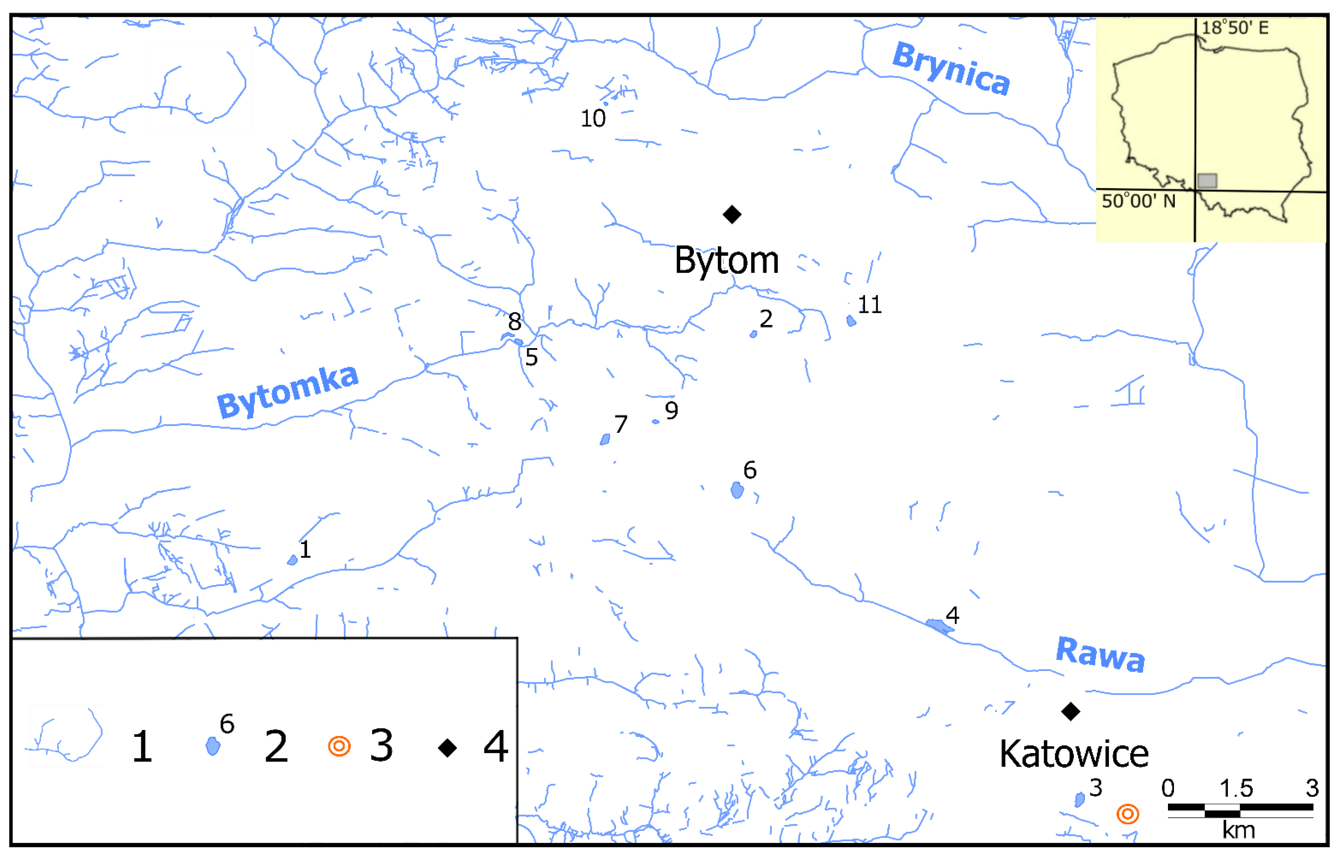
The study covered 11 small anthropogenic water bodies located in the Katowice Upland (Figure 1). The water bodies selected for the study have small surface areas and depths, which translate into small volumes of water retained. The studied water bodies emerged as a result of either intentional or unintentional human activities, and are all classified as endorheic and polymictic (Table 1). The selection of water bodies with similar surface areas, volumes, depths, hydrological characteristics, and mixing patterns was dictated by the desire to reduce the number of factors that could affect the thickness of the forming ice cover; water bodies into which warmer mine waters or river waters burdened with thermal pollutants flowed, which could inhibit ice cover development in such small water bodies, were not selected [26,53]. Endorheic and polymictic water bodies with small surface areas and volumes freeze almost simultaneously, which is also reflected in further changes in ice thickness and the ability to conduct objective observations [11,17].
The study was conducted during three winter seasons: 2009/2010, 2010/2011, and 2011/2012. Ice thickness measurements were conducted frequently: every two days during water body freezing and thawing, and every four days during the period when the ice cover persisted. During winter season 2011/2012, in two water bodies (Amendy and Żabie Doły S), ice thickness measurements were conducted every day from the date that ice phenomena started until they ended. The measurements were performed in the traditional manner, using an ice drill and a measuring staff with a millimetre scale [54,55]. The thickness of both the ice and the snow layer accumulated thereon were observed.
Ice thickness data obtained from field measurements were compared with the ice thickness values obtained from modelling. Two simple empirical models based on the accumulated freezing degree-day formula were used in the study [51,52].
The first model used was the formula put forward by Zubov [52] (Equation (1)):
where:
- h—final ice thickness [cm];
- h0—initial ice thickness [cm];
- ∑(−Tp)—the sum of negative air temperatures counted during the ice accumulation period [°C].
The second model used was the Stefan [51] formula as modified by Michel [32] and Latosri et al. [34] (Equation (2)):
where:
- η—maximum ice thickness during the season [cm];
- αh—empirical coefficient ranging from 0.014–0.017 m/°C−1/2·day1/2;
- S—accumulated freezing degree-days (AFDD).
Originally, both models were used to predict maximum sea ice thickness.
Data on air temperatures were obtained from the meteorological station of the Institute of Meteorology and Water Management in Katowice-Muchowiec.
3. Results
3.1. Meteorological Features
The three consecutive winter seasons included in the study were characterised by quite different weather conditions, which translated into different conditions in which ice covers formed, persisted, and disappeared in the water bodies covered by the study.
During the 2009/2010 season included in the study, negative mean air temperature values were present for 73 days. Low daily air temperature values (below −10 °C) only persisted for 10 days. There were two brief thaw events during that season: the first was in the third decade of December, and the second lasted from the end of the second decade of February until early March. The sum of negative air temperature values during that season was −411.6.
In the 2010/2011 winter season, negative mean air temperature values were present for 72 days and low air temperature values persisted for 4 days. In that season, seven episodes with positive air temperatures were recorded, with the shortest two lasting two days each (in the first decade of December and in the second decade of February), and the longest one lasting almost two weeks (from 7 to 19 January). The sum of negative temperature values from the start until the end of the ice phenomena was −338.7.
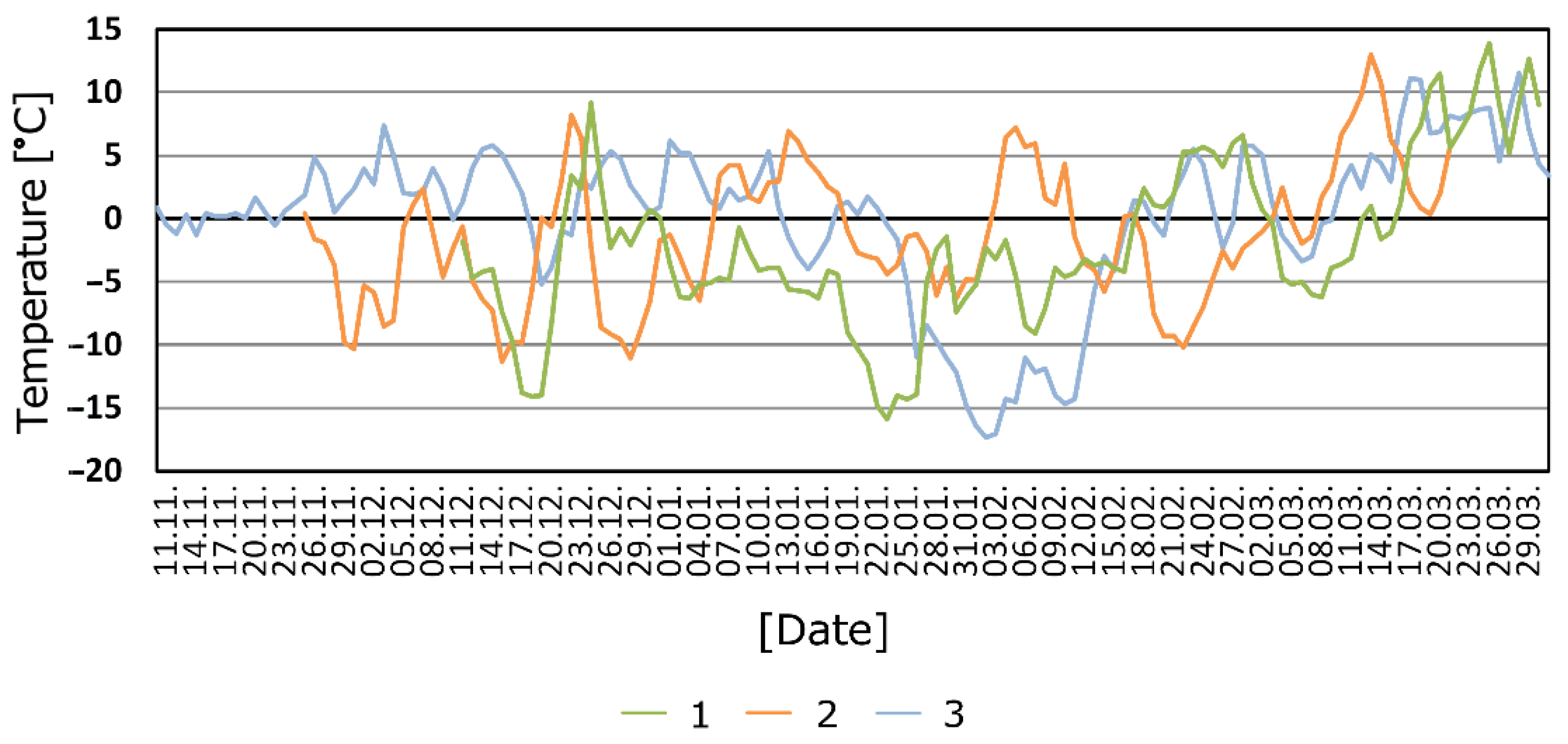
In the 2011/2012 winter season, negative mean air temperature values were present for 48 days and very low air temperatures persisted for 15 days. In the first part of this season (from 11 November to 13 January), air temperatures oscillated around 0 °C, which favoured the rapid emergence and disappearance of ice phenomena on the water bodies which were studied. A significant drop in air temperature did not occur until the second half of January and it lasted for 35 days (Figure 2). In the third study season, the sum of negative temperature values was −296.4.
3.2. Snow Conditions
Snow conditions during the three seasons in which measurements were conducted varied (Table 2).
During the first study season, the average thickness of snow accumulated on the ice cover ranged from 4.1 cm to 7.9 cm with a mean of 5.2 cm. During that period, the maximum snow thickness ranged from 7.0 to 16.5 cm with a mean of 13.0 cm (Table 2). Snow cover thickness steadily increased during the winter season, reaching its maximum at the end of the first and at the beginning of the second decade of February. This was followed by a rapid decline in snow thickness.
In the second study season, the snow accumulated on the ice covering the water bodies was slightly thinner. The average thickness ranged from 2.5 cm to 4.6 cm with a mean of 3.7 cm, and the maximum snow thickness ranged from 6.0 to 11.0 cm with a mean of 9.0 cm (Table 2). During that study season, the thickest snow cover was recorded in the first part of the season (December), and, thereafter, a gradual decrease in snow thickness followed.
During the third study season, the average snow thickness ranged from 1.4 cm to 5.0 cm with a mean of 2.8 cm. The maximum snow cover thickness ranged from 4.0 cm to 21.5 cm with a mean of 11.0 cm (Table 2). During that season, thick snow only lasted for a short time, from late January until mid-February.
3.3. Ice Cover Thickness
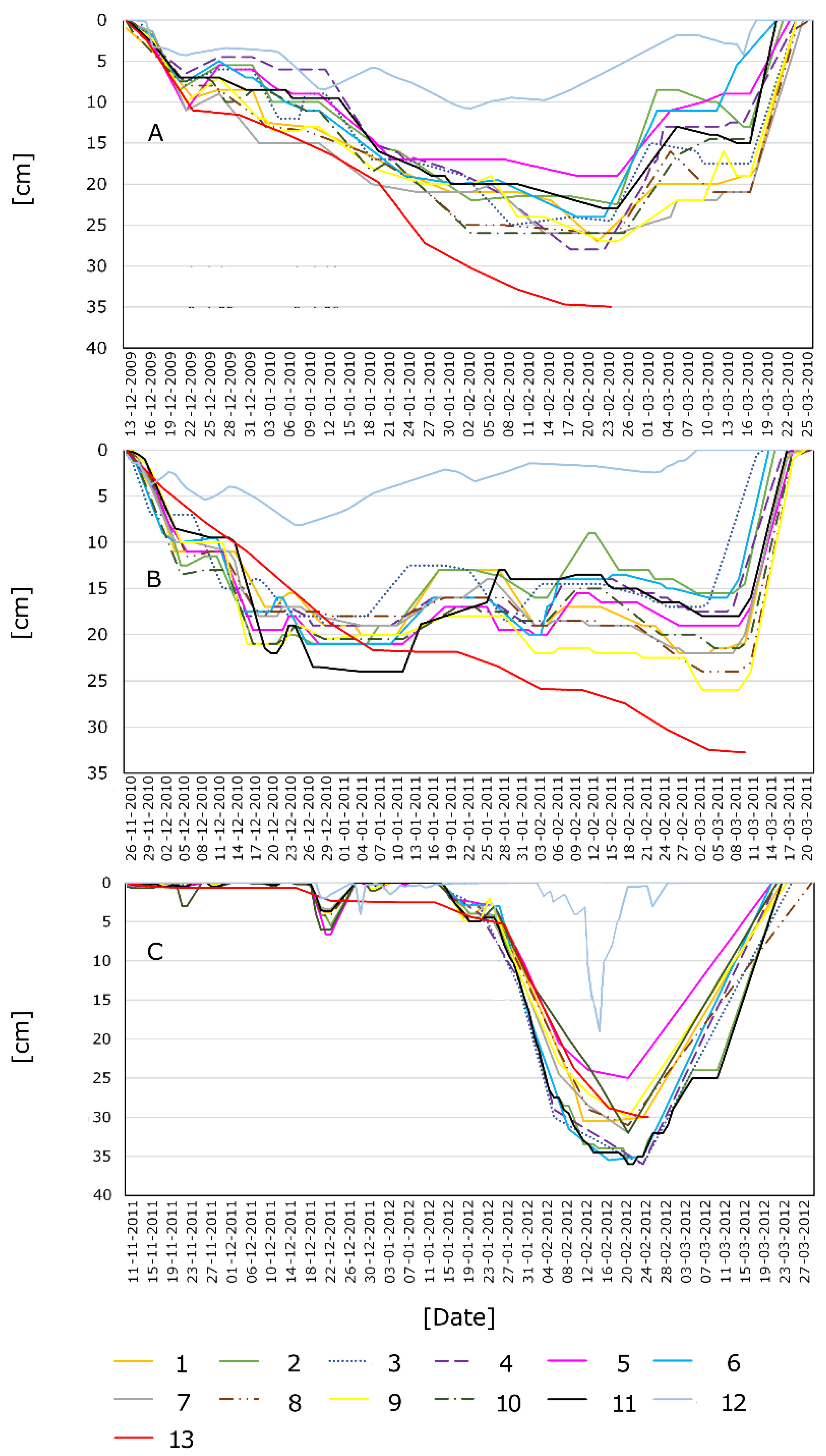
Ice cover thickness during the three seasons in which measurements were conducted varied (Table 3, Figure 3 and Figure 4).
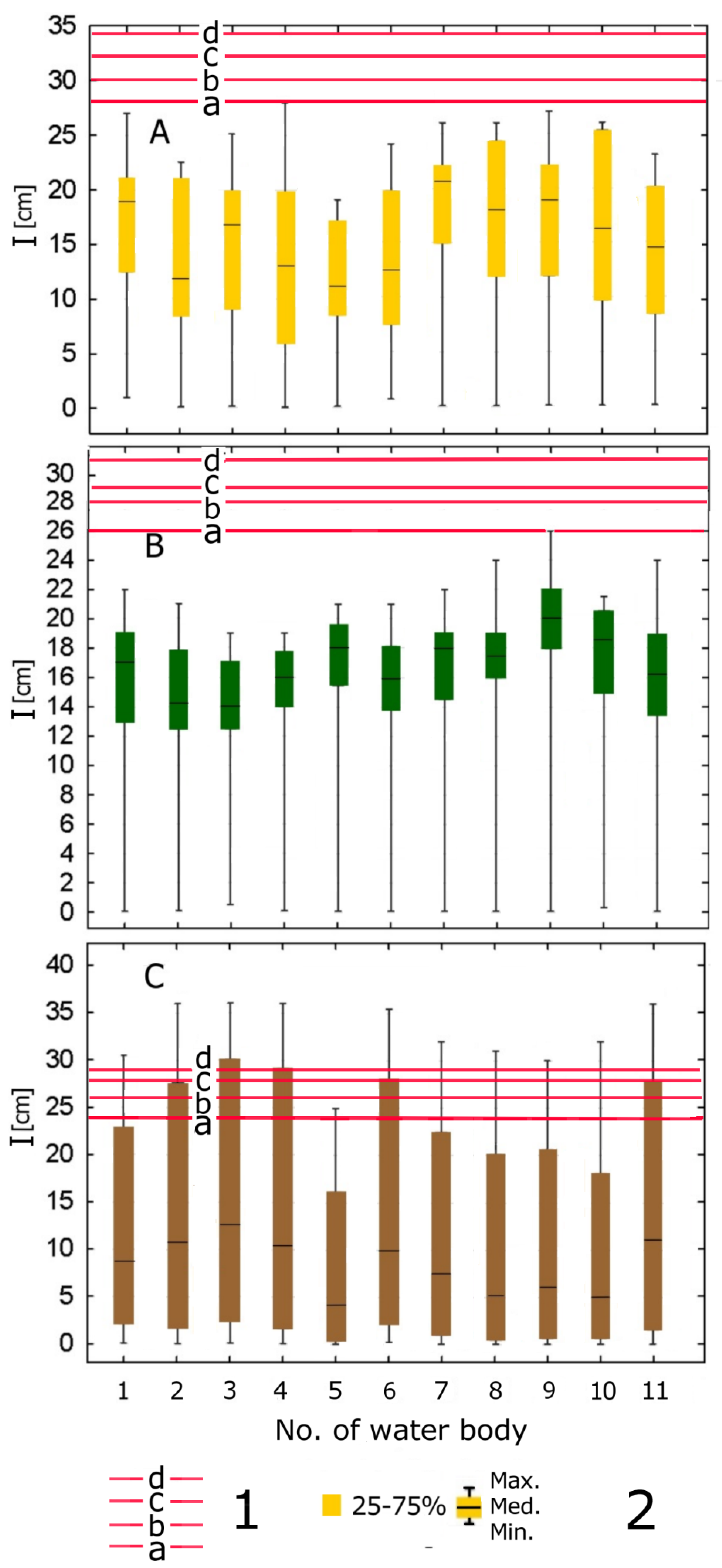
In the 2009/2010 winter season, the differences between the maximum ice thickness values observed and the maximum thickness values obtained by modelling using Zubov’s formula ranged from 7.0 cm (Maroko) to 16.0 cm (Rozlewisko Bytomki) with a mean of 10.0 cm (Figure 3, Table 3). A better fit between the model and the values observed was obtained using Stefan’s formula. In this case, the maximum thickness values modelled ranged from 28 cm to 34 cm depending on the coefficient which was adopted (Figure 4). The closest fit was obtained using a coefficient of 0.014. In this case, the differences between the thickness values observed and modelled ranged from 0.0 cm (Maroko) to 9.0 cm (Rozlewisko Bytomki) with a mean of 3.0 cm.
In the 2010/2011 winter season, the differences between the maximum ice thickness values observed and the maximum thickness values obtained by modelling using Zubov’s formula ranged from 7.0 cm (Trupek) to 14.0 cm (Grunfeld, Maroko) with a mean of 11.0 cm (Figure 3, Table 3). A better fit between the model and the values observed was obtained using Stefan’s formula. In this case, the maximum thickness values modelled ranged from 26 cm to 31 cm (Figure 4), and the differences between them and the values observed ranged from 4.0 cm to 9.0 cm on average. Again, the closest fit was obtained using a coefficient of 0.014. In this case, the differences between the thickness values observed and modelled ranged from 0.0 cm (Trupek) to 7.0 cm (Grunfeld, Maroko) with a mean of 4.0 cm (Table 3).
In the 2011/2012 winter season, the differences between the maximum ice thickness values observed and the maximum thickness values obtained by modelling using Zubov’s formula ranged from 0.0 cm (Trupek) to 6.0 cm (Amendy, Grunfeld, Maroko, Żabie Doły S) with a mean of 3.6 cm (Figure 3, Table 3). In the 2011/2012 winter season, in nine cases, the values modelled were lower than those observed. For Stefan’s formula, a better fit between the values observed and modelled was obtained for higher coefficient values (0.016–0.017) (Figure 4). On average, differences between the values observed and modelled ranged from 2.6 cm (for a coefficient of 0.016) to 8.0 cm (for a coefficient of 0.014). The maximum ice thickness values derived from the modelling were generally lower than the values which were observed (for coefficient values within the 0.014–0.017 range).
4. Discussion
Maximum ice thickness values usually occur in the second part of the winter season as a result of the gradual accretion of crystalline ice from below (in the first part of winter) followed by snow ice accretion from above [18,26,56]. The dynamics of both these processes determine the final thickness of the ice cover formed on the water body. Therefore, the most important factors that affect final ice thickness include air temperatures in the immediate vicinity of the water body, the amount of heat accumulated in the water and bottom sediments after the summer season, and the thickness of snow accumulated on the ice cover during the winter.
The three winter seasons which were studied differed in terms of the prevailing air temperatures and snowfall. During the first season, the ice cover grew gradually to reach its greatest thickness in late February. Almost from the very beginning of the ice phenomena, a thin (a few centimetres thick) layer of snow lay on the ice cover, which grew until the second half of February, reaching a dozen or so centimetres on most of the examined water bodies. Thus, ice accretion in the first part of the winter was inhibited by the layer of snow present on the ice, and when a thick layer of snow accumulated on the ice cover, the accretion of snow ice from above was triggered. The maximum ice thickness values which were observed differed significantly from those obtained from modelling using Zubov’s formula, which does not account for the snow layer that accumulates on the ice during winter. A better fit was obtained for Stefan’s formula, which is mainly due to the fact that it takes into account the role of snow cover in ice cover accretion; the smallest differences between the values observed and modelled were obtained for a coefficient of 0.014. During the second winter season, ice phenomena on water bodies persisted for a long period. At the same time, that winter was milder with periods of lower air temperatures interspersed with thaw episodes. In total, during the period when ice phenomena were present, there were as many as seven periods with positive mean daily air temperatures, which ranged from two days to almost two weeks in duration. A thick ice cover played a part in the vertical development of the ice cover from the beginning of that season. The maximum thickness of the snow accumulated on the ice cover in all studied water bodies was observed in the first part of the season (in December). The dynamics of ice thickness growth in the studied water bodies varied. In five water bodies, the maximum value was observed at the beginning of winter, while, in six, it was reached only at the end of the season. The maximum ice thickness values observed were smaller than the maximum thickness obtained using Zubov’s model by as much as 11 cm, which is mainly due to the fact that ice cover accretion at the beginning of the season was inhibited by the layer of snow accumulated thereon. Nevertheless, an important factor limiting the vertical development of the ice cover was the air temperatures during winter. Ice covers accumulated and melted several times as a result of thaw events. A much better fit of the values modelled was obtained using Stefan’s formula with the coefficient set at the levels of 0.014 and 0.015. In this case, the ice thickness values modelled were only overestimated by four centimetres (0.014) and six centimetres (0.015) on average.
The third winter season was the longest; however, at the same time, negative mean air temperatures persisted for only about one-third of the time during which ice phenomena were present. During the first two months of the season (from 11 November to 13 January), the mean daily air temperature oscillated around 0 °C, which resulted in the water bodies fully freezing and subsequently thawing several times. At that time, ice thickness did not exceed a few centimetres. A significant drop in temperature occurred in mid-January, with mean daily values remaining below −10 °C for more than two weeks. Subsequently, the air temperature started to gradually rise in late February. During that study season, no thick snow layer affected ice cover accretion in general. A snow cover of around a dozen centimetres persisted on the ice covers for almost two weeks; however, that was at a time when the ice covers had already reached their maximum thickness. The values modelled using both Zubov’s formula and Stefan’s model were slightly lower than the maximum observed ice thickness values. The maximum ice thickness modelled using Zubov’s formula was 30 cm, which was, on average, 2.7 cm lower than the thickness values observed in the water bodies. The best ice thickness fit was once again obtained using Stefan’s formula. The maximum ice thickness calculated using this model, with a coefficient of 0.016, was, on average, only 2.6 cm lower than the values observed. Slightly larger differences were noted for a coefficient of 0.017 (an average of 2.8 cm). Ice thickness was underestimated by much more when coefficients of 0.014 and 0.015 were used—by 8 cm and 6 cm, respectively. The fact that Zubov’s model achieved a much better fit in that season was due to the small contribution of snow cover—it first contributed to inhibiting ice cover growth and then to its accretion from above. For Stefan’s formula, higher coefficient values of 0.016 and 0.017 produced much better results than in the previous two study seasons.
5. Conclusions
In the study, two simple models were used to estimate the maximum thickness of ice forming on water bodies. These are based primarily on the accumulated freezing degree-days formula. The model fits varied across the winter seasons. In the first winter season, the ice thickness modelled by Zubov’s formula was, on average, 10 cm greater than the values observed; the difference represented on average 40% of the maximum ice thickness values observed in that season. The values obtained using Stefan’s formula were overestimated by between three and nine centimetres; the difference represented on average between 13 and 37% of the maximum ice thickness values observed. In the second winter season, ice thickness values modelled using Zubov’s formula were overestimated by an average of 11 cm, which represented, on average, 51% of the maximum ice thickness values observed in that season. Again, a much better model fit was obtained using Stefan’s formula, with the ice thickness values obtained using this formula overestimated by an average of four to nine centimetres, i.e., 19 to 42% of the maximum ice thickness values observed in that season. The best fit between Zubov’s model and the thickness values observed was obtained in the third study season. In this case, the modelled values were underestimated by an average of 3.6 cm, which represented, on average, 11% of the maximum ice thickness values observed during that season. A better fit between the model and the observed values was obtained using Stefan’s formula, but only for higher coefficient values (0.016 and 0.017), in which case the model’s underestimation was 2.6 cm and 2.8 cm, or 8% and 9% of the maximum ice thickness, respectively. Much poorer fits were obtained for coefficients of 0.014 and 0.015. In this case, the modelled ice thickness values were underestimated by 25% and 19% of the maximum ice thickness, respectively.
The study demonstrates that Stefan’s formula is the model that produces better empirically-validated results. During snowy winters, a better fit between the model and empirical results was obtained using lower coefficients (0.014 and 0.015), and during winters in which the effect of snow on ice cover accretion was negligible, a good fit was obtained using higher coefficient values (0.016 and 0.017). Zubov’s formula may be useful for estimating ice thickness in seasons when no thick snow cover is present on the ice. In general, both models may be useful for estimating ice thickness when the range of data used by more extensive models such as CLimo, FLake, MinLake, or BW88 is not available.
Author Contributions
M.S. and M.R. conceived and planned the study, conducted field work and analyzed the results, and wrote the paper. M.S. and M.R. collaborated on manuscript editing at all stages. All authors have read and agreed to the published version of the manuscript.
Funding
This research was funded by University of Silesia in Katowice (Poland)—Institute of Earth Sciences (project no. WNP/INoZ/2020_ZB25) and Institute of Social and Economic Geography and Spatial Management.
Institutional Review Board Statement
Not applicable.
Informed Consent Statement
Not applicable.
Data Availability Statement
Not applicable.
Acknowledgments
We would like to thank Łukasz Potempka for consulting on the statistical methods applied.
Conflicts of Interest
The authors declare no conflict of interest.
References
- Ashton, G.D. River and lake ice thickening, thinning, and snow ice formation. Cold Reg. Sci. Technol. 2011, 68, 3–19. [Google Scholar] [CrossRef]
- Bengtsson, L. Ice covered lakes. In Encyclopedia of Lakes and Reservoirs; Bengtsson, L., Herschy, R.W., Fairbridge, R.W., Eds.; Springer: New York, NY, USA, 2012; pp. 357–360. [Google Scholar]
- Choiński, A. Physical Limnology of Poland; Adam Mickiewicz University Press Publ.: Poznań, Poland, 2007. [Google Scholar]
- Kirillin, G.; Leppäranta, M.; Terzhevik, A.; Granin, N.; Bernhardt, J.; Engelhardt, C.H.; Efremova, T.; Golosov, S.; Palshin, N.; Sherstyankin, P.; et al. Physics of seasonally ice-covered lakes: A review. Aquat. Sci. 2012, 74, 659–682. [Google Scholar] [CrossRef]
- Skowron, R. The Differentiation and the Changeability of Chosen of Elements the Thermal Regime of Water in Lakes on Polish Lowland; Wydawnictwo Uniwersytetu M. Kopernika: Toruń, Poland, 2011; p. 345. [Google Scholar]
- Solarski, M.; Szumny, M. Conditions of spatiotemporal variability of the thickness of the ice cover on lakes in the Tatra Mountains. J. Mt. Sci. 2020, 17, 2369–2386. [Google Scholar] [CrossRef]
- Livingstone, D.M.; Adrian, R.; Blencknert, T.; George, G.; Weyhenmeyer, G.A. Lake ice phenology. In The Impact of Climate Change on European Lakes 4; George, G., Ed.; Aquatic Ecology Series; Springer: Dordrecht, The Netherlands, 2010; pp. 51–62. [Google Scholar]
- Skowron, R. Differences in thermal and ice regimes formation in lakes Gopło and Bachotek. Limnol. Rev. 2006, 6, 255–262. [Google Scholar]
- Skowron, R. Changeability of the ice cover on the lakes of northern Poland in the light of climatic changes. Bull. Geogr.—Phys. Geogr. 2009, 1, 103–124. [Google Scholar] [CrossRef] [Green Version]
- Aihara, M.; Chikita, K.A.; Momoki, Y.; Mabuchi, S. A physical study on the thermal ice ridge in a closed deep lake: Lake Kuttara, Hokkaido, Japan. Limnology 2010, 11, 125–132. [Google Scholar] [CrossRef] [Green Version]
- Bengtsson, L. Ice formation on lakes and ice growth. In Encyclopedia of Lakes and Reservoirs; Bengtsson, L., Herschy, R.W., Fairbridge, R.W., Eds.; Springer: New York, NY, USA, 2012; pp. 360–361. [Google Scholar]
- Brown, L.C.; Duguay, C.R. The fate of lake ice in the North American Arctic. Cryosphere Discuss 2011, 5, 1775–1834. [Google Scholar] [CrossRef] [Green Version]
- Gao, S.B.; Stefan, H.G. Multiple linear regression for lake ice and lake temperature characteristics. J. Cold Reg. Eng. 1999, 13, 59–77. [Google Scholar] [CrossRef]
- Launiainen, J.; Cheng, B. Modelling of ice thermodynamics in natural water bodies. Cold Reg. Sci. Technol. 1998, 27, 153–178. [Google Scholar] [CrossRef]
- Leppäranta, M. A growth model for black ice, snow ice and snow thickness in subarctic basins. Nord. Hydrol. 1983, 14, 59–70. [Google Scholar] [CrossRef]
- Richards, T.O. The meteorological aspects of ice cover on the Great Lakes. Mon. Weather Rev. 1964, 92, 297–302. [Google Scholar] [CrossRef]
- Solarski, M.; Pradela, A.; Rzetala, M. Natural and anthropogenic influences on ice formation on various water bodies of the Silesian Upland (southern Poland). Limnol. Rev. 2011, 11, 33–44. [Google Scholar] [CrossRef] [Green Version]
- Solarski, M. The ice phenomena dynamics of small anthropogenic water bodies in the Silesian Upland, Poland. Environ. Socio-Econ. Stud. 2017, 5, 74–81. [Google Scholar] [CrossRef] [Green Version]
- Marszelewski, W.; Skowron, R. Spatial diversity of the ice cover on the lakes of the European Lowland in the winter season 2003/2004. Limnol. Rev. 2005, 5, 155–165. [Google Scholar]
- Choiński, A.; Ptak, M.; Skowron, R.; Strzelczak, A. Changes in ice phenology on Polish lakes from 1961 to 2010 related to location and morphometry. Limnologica 2015, 53, 42–49. [Google Scholar] [CrossRef]
- Chen, C.V.; Weintraub, L.H.Z.; Herr, J.; Goldstein, R.A. Impacts of a thermal power plant on the phosphorus TMDL of a reservoir. Environ. Sci. Policy 2000, 3, 217–223. [Google Scholar] [CrossRef]
- Eloranta, P.V. Physical and chemical properties of pond waters receiving warm water effluent from a thermal power plant. Water Res. 1983, 17, 133–140. [Google Scholar] [CrossRef]
- Machowski, R. Course of ice phenomena in small water reservoir in Katowice (Poland) in the winter season 2011/2012. Environ. Socio-Econ. Stud. 2013, 1, 7–13. [Google Scholar] [CrossRef] [Green Version]
- Rzetala, M. Ice cover development in a small water body in an undrained depression. In Proceedings of the International Multidisciplinary Scientific Geoconference, 14th GeoConference on Water Resources. Forest, Marine and Ocean Ecosystems SGEM, Albena, Bulgary, 17–26 June 2014; pp. 397–404. [Google Scholar] [CrossRef]
- Rzętała, M. Functioning of Water Reservoirs and the Course of Limnic Processes under Conditions of Varied Anthropopression a Case Study of Upper Silesian Region; University of Silesia: Katowice, Poland, 2008; pp. 1–172. [Google Scholar]
- Solarski, M.; Rzetala, M. Changes in the Thickness of Ice Cover on Water Bodies Subject to Human Pressure (Silesian Upland, Southern Poland). Front. Earth Sci. 2021, 9, 675216. [Google Scholar] [CrossRef]
- Solarski, M.; Rzetala, M. Ice Regime of the Kozłowa Góra Reservoir (Southern Poland) as an Indicator of Changes of the Thermal Conditions of Ambient Air. Water 2020, 12, 2435. [Google Scholar] [CrossRef]
- Noori, R.; Bateni, S.M.; Saari, M.; Almazroui, M.; Haghighi, A.T. Strong Warming Rates in the Surface and Bottom Layers of a Boreal Lake: Results From Approximately Six Decades of Measurements (1964–2020). Earth Space Sci. 2022, 9, 1–14. [Google Scholar] [CrossRef]
- Noori, R.; Woolway, R.I.; Saari, M.; Pulkkanen, M.; Klove, B. Six Decades of Thermal Change in a Pristine Lake Situated North of the Arctic Circle. Water Resour. Res. 2022, 58, 2021WR031543. [Google Scholar] [CrossRef]
- Jones, P.D.; Osborn, T.J.; Briffa, K.R. The evolution of climate over the last millennium. Science 2001, 292, 662–667. [Google Scholar] [CrossRef] [Green Version]
- Degirmendzic, J.; Rozuchowski, K.; Zmudzka, E. Changes of air temperature and precipitation in Poland in the period 1951–2000 and their relationship to atmospheric circulation. Int. J. Climatol. 2004, 24, 291–310. [Google Scholar] [CrossRef]
- Michel, B. Winter Regime of River and Lakes. In Cold Regions Science and Engineering Monograph III-B1a; U.S. Army Cold Regions Research and Engineering Laboratory: Hanover, NH, USA, 1971; pp. 1–131. [Google Scholar]
- DEBruijn, E.I.F.; Bosveld, F.C.; Van Der Plas, E.V. An intercomparison study of ice thickness models in the Netherlands. Tellus A Dyn. Meteorol. Oceanogr. 2014, 66, 21244. [Google Scholar] [CrossRef] [Green Version]
- Lotsari, E.; Lind, L.; Kämäri, M. Impacts of Hydro-Climatically Varying Years on Ice Growth and Decay in a Subarctic River. Water 2019, 11, 2058. [Google Scholar] [CrossRef] [Green Version]
- Barańczuk, J.; Barańczuk, K. Models for calculating ice cover thickness on selected endorheic lakes of the upper Radunia (Kashubian Lakeland, northern Poland). Limnol. Rev. 2018, 18, 129–135. [Google Scholar] [CrossRef] [Green Version]
- Ménard, P.; Duguay, C.R.; Flato, G.M.; Rouse, W.R. Simulation of ice phenology on Great Slave Lake, Northwest Territories, Canada. Hydrol. Process. 2002, 16, 3691–3706. [Google Scholar] [CrossRef]
- Duguay, C.R.; Flato, G.M.; Jeffries, M.O.; Ménard, P.; Morris, K.; Rouse, W.R. Ice-cover variability on shallow lakes at high latitudes: Model simulations and observations. Hydrol. Process. 2003, 17, 3465–3483. [Google Scholar] [CrossRef]
- Jeffries, M.O.; Morris, K.; Duguay, C.R. Lake ice growth and decay in central Alaska, USA: Observations and computer simulations compared. Ann. Glaciol. 2005, 40, 195–199. [Google Scholar] [CrossRef] [Green Version]
- Morris, K.; Jeffries, M.; Duguay, C. Model simulation of the effects of climate variability and change on lake ice in central Alaska, USA. Ann. Glaciol. 2005, 40, 113–118. [Google Scholar] [CrossRef]
- Kheyrollah-Pour, H.; Duguay, C.R.; Martynov, A.; Brown, L.C. Simulation of surface temperature and ice cover of large northern lakes with 1-D models: A comparison with MODIS satellite data and in situ measurements. Tellus A 2012, 64, 17614. [Google Scholar] [CrossRef]
- Fang, X.; Stefan, H.G. Simulations of climate effects on water temperature, dissolved oxygen, ice and snow covers in lakes of the Contiguous United States under past and future climate scenarios. Limnol. Oceanogr. 2009, 54, 2359–2370. [Google Scholar] [CrossRef]
- Dibike, Y.; Prowse, T.; Saloranta, T.; Ahmed, R. Response of Northern Hemisphere lake-ice cover and lake-water thermal structure patterns to a changing climate. Hydrol. Process. 2011, 25, 2942–2953. [Google Scholar] [CrossRef]
- Dibike, Y.; Prowse, T.; Bonsal, B.; DERham, L.; Saloranta, T. Simulation of North American lake-ice cover characteristics under contemporary and future climate conditions. Int. J. Climatol. 2012, 32, 695–709. [Google Scholar] [CrossRef]
- Bernhardt, J.; Engelhardt, C.H.; Kirillin, G.; Matschullat, J. Lake ice phenology in Berlin-Brandenburg from 1947–2007: Observations and model hindcasts. Clim. Chang. 2011, 112, 791–817. [Google Scholar] [CrossRef]
- Vavrus, S.J.; Wynne, R.H.; Foley, J.A. Measuring the sensitivity of southern Wisconsin lake ice to climate variations and lake depth using a numerical model. Limnol. Oceanogr. 1996, 41, 822–831. [Google Scholar] [CrossRef]
- Walsh, S.E.; Vavrus, S.J.; Foley, J.A.; Fisher, V.A.; Wynne, R.H.; Lenters, J.D. Global patterns of lake ice phenology and climate: Model simulations and observations. J. Geophys. Res. Atmos. 1998, 103, 28825–28837. [Google Scholar] [CrossRef] [Green Version]
- Wang, J.; Duguay, C.R.; Clausi, D.A.; Pinard, V.; Howell, S.E.L. Semi-Automated Classification of Lake Ice Cover Using Dual Polarization RADARSAT-2 Imagery. Remote Sens. 2018, 10, 1727. [Google Scholar] [CrossRef] [Green Version]
- Cai, Y.; Duguay, C.R.; Ke, C.-Q. A 41-year (1979–2019) passive-microwave-derived lake ice phenology data record of the Northern Hemisphere. Earth Syst. Sci. Data 2022, 14, 3329–3347. [Google Scholar] [CrossRef]
- Knoll, L.B.; Sharma, S.; Denfeld, B.A.; Flaim, G.; Hori, Y.; Magnuson, J.J.; Straile, D.; Weyhenmeyer, G.A. Consequences of lake and river ice loss on cultural ecosystem services. Limnol. Oceanogr. Lett. 2019, 4, 119–131. [Google Scholar] [CrossRef]
- Sharma, S.; Blagrave, K.; Watson, S.R.; O’Reilly, C.M.; Batt, R.; Magnuson, J.J.; Clemens, T.; Denfeld, B.A.; Flaim, G.; Grinberga, L.; et al. Increased winter drownings in ice-covered regions with warmer winters. PLoS ONE 2020, 15, e0241222. [Google Scholar] [CrossRef]
- Stefan, J. Ueber die Theorie der Eisbildung, insbesondere über die Eisbildung im Polarmeere. Ann. Der Phys. 1891, 278, 269–286. [Google Scholar] [CrossRef] [Green Version]
- Zubov, N.N. L’dy Arktiki (Arctic Ice); Izdatel’stvo Glavsevmorputi: Moscow, Russia, 1945. [Google Scholar]
- Stigebrandt, A. Dynamics of an Ice Covered Lake with Through-Flow. Hydrol. Res. 1978, 9, 219–244. [Google Scholar] [CrossRef]
- Doesken, N.J.; Judson, A. The Snow Booklet: A Guide to the Science, Climatology and Measurements of Snow in the United States, 2nd ed.; Colorado State University: Fort Collins, CO, USA, 1996; p. 85. [Google Scholar]
- Pirazzini, R.; Leppänen, L.; Picard, G.; Lopez-Moreno, J.I.; Marty, C.; Macelloni, G.; Kontu, A.; Von Lerber, A.; Tanis, C.M.; Schneebeli, M.; et al. European In-Situ Snow Measurements: Practices and Purposes. Sensors 2018, 18, 2016. [Google Scholar] [CrossRef]
- Leppäranta, M. Freezing of Lakes and the Evolution of Their Ice Cover; Springer: Berlin, Germany, 2015. [Google Scholar]
Figure 1.
Location of the anthropogenic water bodies studied in the Katowice Upland (southern Poland): 1—rivers; 2—water bodies studied (numbering as in Table 1); 3—meteorological station; 4—major towns.
Figure 1.
Location of the anthropogenic water bodies studied in the Katowice Upland (southern Poland): 1—rivers; 2—water bodies studied (numbering as in Table 1); 3—meteorological station; 4—major towns.

Figure 2.
Average air temperature values in the ice phenomena period for the winter seasons studied: 2009–2010 (1), 2010–2011 (2), and 2011–2012 (3).
Figure 2.
Average air temperature values in the ice phenomena period for the winter seasons studied: 2009–2010 (1), 2010–2011 (2), and 2011–2012 (3).

Figure 3.
Maximum thickness of ice on water bodies in Katowice Upland in 2009/2010, 2010/2011, and 2011/2012 winter seasons—observed and modelled values: (A)—2009/2010 winter season; (B)—2010/2011 winter season; (C)—2011/2012 winter season; 1–11—ice thickness observed in water bodies (water body numbering as in Table 3); 12—snow cover thickness, 13—maximum ice thickness according to Zubov’s formula.

Figure 4.
Ice thickness on the water bodies of the Silesian Upland in the (A) first, (B) second, and (C) third winter season: I—ice thickness; No. of water body—ordinal number (numbering as in Table 3). 1—the maximum ice thickness values obtained from modelling using Stefan’s equation (coefficient values: a—0.014, b—0.015, c—0.016, d—0.017); 2—statistical parameters.


Table 1.
Certain morphogenetic and hydrological parameters of the selected water bodies in the Katowice Upland.
Table 1.
Certain morphogenetic and hydrological parameters of the selected water bodies in the Katowice Upland.
| No. | Water Body | Altitude [m a.s.l.] | A [ha] | Davg [m] | V [103 m3] | O | H | M |
|---|---|---|---|---|---|---|---|---|
| 1 | Akwen | 241.0 | 2.4 | 2.6 | 62.3 | Pe | B | P |
| 2 | Amendy | 287.7 | 1.3 | 1.6 | 21.4 | Pe | B | P |
| 3 | Grunfeld | 290.0 | 3.9 | 4.6 | 179.0 | Pe | B | P |
| 4 | Maroko | 264.9 | 8.1 | 1.4 | 109.5 | Pg | B | P |
| 5 | Rozlewisko Bytomki | 243.0 | 1.2 | 1.2 | 14.3 | N | B | P |
| 6 | Skałka | 276.1 | 5.9 | 1.9 | 110.3 | S | B | P |
| 7 | Smrodlok | 284.5 | 2.9 | 1.6 | 46.4 | N | B | P |
| 8 | Szkopka | 245.2 | 1.4 | 1.6 | 21.8 | Pg | B | P |
| 9 | Trupek | 288.0 | 0.7 | 1.2 | 8.1 | Pe | B | P |
| 10 | Zbiornik przy Leśnej | 259.4 | 0.3 | 0.7 | 2.0 | N | B | P |
| 11 | Żabie Doły S | 278.0 | 2.6 | 1.7 | 43.3 | N | B | P |
Notes: A—area; Davg—Average depth; V—Volume; O—Origin (N—subsidence bowl; Pg—polygenetic; Pe—former extraction pit; S—artifical bowl; H—Hydrological type (B—non-drained); M—Mixing type (P—polymictic).
Table 2.
Average (AT) and maximal (MT) snow cover thickness values on studied water bodies of Katowice Upland in the winter seasons of 2009/2010, 2010/2011, and 2022/2012 ([26] simplified).
Table 2.
Average (AT) and maximal (MT) snow cover thickness values on studied water bodies of Katowice Upland in the winter seasons of 2009/2010, 2010/2011, and 2022/2012 ([26] simplified).
| No. | Water Body | Season I (2009/2010) | Season II (2010/2011) | Season III (2011/2012) | |||
|---|---|---|---|---|---|---|---|
| AT | MT | AT | MT | AT | MT | ||
| [cm] | |||||||
| 1 | Akwen | 7.8 | 15.0 | 3.8 | 8.0 | 4.7 | 21.5 |
| 2 | Amendy | 6.3 | 10.0 | 3.8 | 7.0 | 2.7 | 15.0 |
| 3 | Grunfeld | 4.7 | 15.5 | 3.1 | 9.5 | 1.8 | 8.0 |
| 4 | Maroko | 5.8 | 12.0 | 3.6 | 10.0 | 1.4 | 6.0 |
| 5 | Rozlewisko Bytomki | 5.3 | 12.0 | 3.5 | 6.0 | 2.2 | 6.0 |
| 6 | Skałka | 5.8 | 13.0 | 4.6 | 9.0 | 5.0 | 21.5 |
| 7 | Smrodlok | 6.8 | 17.0 | 4.1 | 11.0 | 2.5 | 8.0 |
| 8 | Szkopka | 4.1 | 7.0 | 3.5 | 8.0 | 2.5 | 7.5 |
| 9 | Trupek | 6.7 | 16.5 | 4.7 | 11.0 | 2.9 | 8.0 |
| 10 | Zbiornik przy Leśnej | 6.5 | 16.5 | 2.5 | 9.0 | 2.1 | 4.0 |
| 11 | Żabie Doły S | 5.1 | 9.0 | 3.8 | 10.0 | 2.5 | 15.5 |
Table 3.
Maximum thickness of ice cover on water bodies in Katowice Upland in 2009/2010–2011/2012 winter seasons.
Table 3.
Maximum thickness of ice cover on water bodies in Katowice Upland in 2009/2010–2011/2012 winter seasons.
| No. | Water Body | Max IT | Max Z | Max S | |||
|---|---|---|---|---|---|---|---|
| 0.014 | 0.015 | 0.016 | 0.017 | ||||
| Season 2009/2010 | |||||||
| 1 | Akwen | 27.0 | 35.0 | 28.0 | 30.0 | 32.0 | 34.0 |
| 2 | Amendy | 23.0 | 35.0 | 28.0 | 30.0 | 32.0 | 34.0 |
| 3 | Grunfeld | 25.0 | 35.0 | 28.0 | 30.0 | 32.0 | 34.0 |
| 4 | Maroko | 28.0 | 35.0 | 28.0 | 30.0 | 32.0 | 34.0 |
| 5 | Rozlewisko Bytomki | 19.0 | 35.0 | 28.0 | 30.0 | 32.0 | 34.0 |
| 6 | Skałka | 24.0 | 35.0 | 28.0 | 30.0 | 32.0 | 34.0 |
| 7 | Smrodlok | 26.0 | 35.0 | 28.0 | 30.0 | 32.0 | 34.0 |
| 8 | Szkopka | 26.0 | 35.0 | 28.0 | 30.0 | 32.0 | 34.0 |
| 9 | Trupek | 27.0 | 35.0 | 28.0 | 30.0 | 32.0 | 34.0 |
| 10 | Zbiornik przy Leśnej | 26.0 | 35.0 | 28.0 | 30.0 | 32.0 | 34.0 |
| 11 | Żabie Doły S | 23.0 | 35.0 | 28.0 | 30.0 | 32.0 | 34.0 |
| Season 2010/2011 | |||||||
| 1 | Akwen | 22.0 | 33.0 | 26.0 | 28.0 | 29.0 | 31.0 |
| 2 | Amendy | 21.0 | 33.0 | 26.0 | 28.0 | 29.0 | 31.0 |
| 3 | Grunfeld | 19.0 | 33.0 | 26.0 | 28.0 | 29.0 | 31.0 |
| 4 | Maroko | 19.0 | 33.0 | 26.0 | 28.0 | 29.0 | 31.0 |
| 5 | Rozlewisko Bytomki | 21.0 | 33.0 | 26.0 | 28.0 | 29.0 | 31.0 |
| 6 | Skałka | 21.0 | 33.0 | 26.0 | 28.0 | 29.0 | 31.0 |
| 7 | Smrodlok | 22.0 | 33.0 | 26.0 | 28.0 | 29.0 | 31.0 |
| 8 | Szkopka | 24.0 | 33.0 | 26.0 | 28.0 | 29.0 | 31.0 |
| 9 | Trupek | 26.0 | 33.0 | 26.0 | 28.0 | 29.0 | 31.0 |
| 10 | Zbiornik przy Leśnej | 22.0 | 33.0 | 26.0 | 28.0 | 29.0 | 31.0 |
| 11 | Żabie Doły S | 24.0 | 33.0 | 26.0 | 28.0 | 29.0 | 31.0 |
| Season 2011/2012 | |||||||
| 1 | Akwen | 30.5 | 30.0 | 24.0 | 26.0 | 28.0 | 29.0 |
| 2 | Amendy | 36 | 30.0 | 24.0 | 26.0 | 28.0 | 29.0 |
| 3 | Grunfeld | 36 | 30.0 | 24.0 | 26.0 | 28.0 | 29.0 |
| 4 | Maroko | 36 | 30.0 | 24.0 | 26.0 | 28.0 | 29.0 |
| 5 | Rozlewisko Bytomki | 25 | 30.0 | 24.0 | 26.0 | 28.0 | 29.0 |
| 6 | Skałka | 36 | 30.0 | 24.0 | 26.0 | 28.0 | 29.0 |
| 7 | Smrodlok | 32 | 30.0 | 24.0 | 26.0 | 28.0 | 29.0 |
| 8 | Szkopka | 31 | 30.0 | 24.0 | 26.0 | 28.0 | 29.0 |
| 9 | Trupek | 30 | 30.0 | 24.0 | 26.0 | 28.0 | 29.0 |
| 10 | Zbiornik przy Leśnej | 32 | 30.0 | 24.0 | 26.0 | 28.0 | 29.0 |
| 11 | Żabie Doły S | 36 | 30.0 | 24.0 | 26.0 | 28.0 | 29.0 |
Notes: Max IT—measured maximum ice thickness (cm); Max Z—maximum ice thickness using Zubov’s formula (cm); Max S—maximum ice thickness usingStefan’s formula (cm), (0.14–0.017—coefficient values).
Publisher’s Note: MDPI stays neutral with regard to jurisdictional claims in published maps and institutional affiliations. |
© 2022 by the authors. Licensee MDPI, Basel, Switzerland. This article is an open access article distributed under the terms and conditions of the Creative Commons Attribution (CC BY) license (https://creativecommons.org/licenses/by/4.0/).
Share and Cite
MDPI and ACS Style
Solarski, M.; Rzetala, M. A Comparison of Model Calculations of Ice Thickness with the Observations on Small Water Bodies in Katowice Upland (Southern Poland). Water 2022, 14, 3886. https://doi.org/10.3390/w14233886
AMA Style
Solarski M, Rzetala M. A Comparison of Model Calculations of Ice Thickness with the Observations on Small Water Bodies in Katowice Upland (Southern Poland). Water. 2022; 14(23):3886. https://doi.org/10.3390/w14233886
Chicago/Turabian StyleSolarski, Maksymilian, and Mariusz Rzetala. 2022. "A Comparison of Model Calculations of Ice Thickness with the Observations on Small Water Bodies in Katowice Upland (Southern Poland)" Water 14, no. 23: 3886. https://doi.org/10.3390/w14233886
Note that from the first issue of 2016, this journal uses article numbers instead of page numbers. See further details here.