An Automated Machine Learning Engine with Inverse Analysis for Seismic Design of Dams

Abstract

This paper proposes a systematic approach for the seismic design of 2D concrete dams. As opposed to the traditional design method which does not optimize the dam cross-section, the proposed design engine offers the optimal one based on the predefined constraints. A large database of about 24,000 simulations is generated based on transient simulation of the dam-foundation-water system. The database includes over 150 various dam shapes, water levels, and material properties, as well as 160 different ground motion records. Automated machine learning (AutoML) is used to generate a surrogate model of dam response as a function of thirty variables. The accuracy of single- and multi-output surrogate models are compared, and the efficiency of the design engine for various settings is discussed. Next, a simple yet robust inverse analysis method is coupled with a multi-output surrogate model to design a hypothetical dam in the United States. Having the seismic hazard scenario, geological survey data, and also the concrete mix, the dam shape is estimated and compared to direct finite element simulation. The results show promising accuracy from the AutoML regression. Furthermore, the design shape from the inverse analysis is in good agreement with the design objectives and also the finite element simulations.

1. Introduction

Seismic design and analysis of concrete dams have been always challenging tasks because multiple factors are involved in performance evaluation [1]. They include, but are not limited to, the semi-unbounded size of the reservoir and foundation rock domains, fluid-structure interaction, wave absorption at the reservoir boundary, water compressibility, foundation rock-structure interaction, spatial variations in ground motion at the dam-foundation interface, and nonlinear damage mechanism of dam concrete. A detailed review of the dynamic analysis of concrete dams can be found in [2]. However, the seismic safety of existing dams is different from the seismic design of new ones. Whereas linear elastic analyses are warranted for design, nonlinear ones must be performed when the complete structural response is desired, the failure load is to be determined as accurately as possible, or the “true” factor of safety must be found [3].

Structural design is founded on verification of the safety inequality: “Demand ≤ Capacity”. This inequality can be interpreted with different engineering response quantities which results in various seismic design philosophies. In a broad classification, the seismic design is force-based, displacement-based, or energy-based. If both sides of safety inequality are written based on forces or moments, the design is force-based, and if displacement or deformation (e.g., deflection, curvature, strain, and rotation) is used, the design is displacement-based. Finally, if energy terms are compared, the design is energy-based [4].

In force-based design, the lateral load-resisting system is designed for an equivalent static force. However, in the displacement-based method, multiple (drift-based) performance levels are checked to ensure the displacement does not exceed the threshold values. In force-based design, the structural system is designed for a single seismic hazard level, i.e., the design basis earthquake (DBE) in which the structure should satisfy the life safety performance objective. However, the satisfaction of one performance level does not guarantee the satisfaction of other (i.e., higher) performance levels too. In contrast, the displacement-based design operates on multiple performance levels to satisfy all of them. It is noteworthy that an earthquake originally imposes energy (and not force) on a structure. Such energy (through the foundation) produces displacement relative to the ground. The forces are indeed the byproduct of such a relative displacement and not the other way around. Therefore, a displacement-based method is straightforward and more detailed.

Concrete gravity dams have traditionally been designed by an extended version of force-based procedure [5,6]. As opposed to framed structures which include only one equivalent lateral force, there are three static lateral forces in dams: (1) the forces associated with the weight of the dam which is obtained as a product of a seismic coefficient ($\alpha \in [0.05–0.10]$) and the weight of the portion of the dam being considered, (2) the forces associated with reservoir hydrodynamic pressure which are obtained as a product of $\alpha$ and a pressure coefficient, ${\alpha }_p$, and (3) the hydrostatic pressure [7]. There are several limitations in this method: the dynamic characteristics of the coupled system, as well as the time and frequency-domain characteristics of the ground motion records, are not considered. The traditional design method has also very conservative criteria: the compressive stress should be limited to 1/4 of the compressive strength, $f_c^{\prime }$, and the tension is usually not permitted, or the allowable tensile stress is very small. In addition, the static sliding and overturning criteria have little meaning in the context of traditional seismic dam design as the oscillatory responses are ignored.

The authors are unaware of any previous attempt at the displacement-based design of concrete dams. The only accessible document is the research by Andonov et al. [8] which proposed to use of a displacement-based method for linear and nonlinear seismic assessment of the existing dams. Beyond the previous classification for seismic design methods, other extensions have been proposed such as performance-based seismic design [9], reliability-based seismic design [10], risk-based seismic design [11], and more recently, the resilience-based seismic design [12]. Despite the availability of such advanced seismic design frameworks, there are rarely used in concrete dam design probably due to the complexity of the numerical model. For example, Ferguson et al. [13] showed the application of the risk-informed design framework for roller-compacted concrete dams under extreme seismic events.

On the other hand, the shape optimization of the existing dam layout has been discussed widely for both gravity and arch dams. The pioneering work belongs to Ramakrishnan and Francavilla [14] that used the penalty function to optimize the shape of gravity dams. Others adopted simple or advanced optimization algorithms for dam shape optimization [15,16,17]. Some others combined the optimization algorithms with machine learning to accelerate the process [18,19]. A risk-based framework for shape optimization of arch dams was introduced by Talatahari et al. [20] on which expected costs of failure are incorporated in the analysis. More recently, a surrogate–assisted shape optimization framework for dams was introduced by Fengjie and Lahmer [21] which incorporates various uncertainty sources. This method has been extended by Abdollahi et al. [22] for multiple seismic performance levels by eliminating the design dependency on a particular ground motion record. Nearly all these techniques require advanced knowledge of optimization techniques and/or machine learning modeling. Moreover, a large number of finite element simulations is required to satisfy the objective functions. Therefore, they are not popular among practitioners. Moreover, a series of particular cost functions are required during the shape optimization such as volume of concrete, construction quality and complexity, location of dam and availability of materials, etc. which makes the generalization of results nearly impossible.

With multiple limitations in the traditional seismic design method, and also the complexity of the advanced shape optimization techniques, there is a need for a simple yet accurate seismic design framework. This paper proposes a finite element-based design engine to assist the practitioners in feasibility level (i.e., initial) layout development for 2D concrete gravity dams under seismic events. The engine includes a large inventory of gravity dam shapes with different material properties for concrete and foundation rock. Such a large inventory has been subjected to different water levels and many ground motion records. The current database covers about 24,000 unique combinations of dam shapes, material properties, water, and earthquake loading. Further, a low-code automated machine learning (AutoML) tool is used to develop a high-fidelity surrogate model that connects all the design variables to response quantities (e.g., displacements and stresses). Such an AutoML surrogate model has never been trained for structural systems (more specifically dams) with both the epistemic (i.e., modeling and material) and aleatory (i.e., loading) variability [23,24]. Therefore, the first contribution of this paper is to explore the accuracy of such a surrogate model with different assumptions that an AutoML prepackage is provided for analysts. Next, a surrogate model-based inverse analysis is introduced for initial parameter estimation during dam design. Using the generated engine in this paper, and also having some information about the seismic event, the engineer will be able to estimate the dam shape for different levels of response quantity in a second. This engine provides the best initial guess (shape and material of the dam) based on the constraints that are introduced by the analyst.

The paper’s structure is as follows: Section 2 provides a quick review of the AutoML and its differences with classical machine learning approaches. Furthermore, a high-level review is provided about the application of machine learning in the seismic analysis of dams. Section 3 provides the underpinning theories about the design variables used in this paper to develop the surrogate models. The data structure is discussed in Section 4 including a brief explanation of the software used for finite element simulations, and also some generic responses from the database. Section 5 dives into the AutoML application, the anatomy, and performance of the developed surrogate models, while Section 6 explores the design engine and inverse problems, as well as some practical examples. Finally, a summary of the research this provided in Section 7.

2. Automated Machine Learning (AutoML)

2.1. ML-Based Response Evaluation of Dams

Most of the current applications of machine learning in dam engineering are focused on structural health monitoring which mainly compiles the measured data during the lifetime of the dam and predicts the response trend [25,26]. This is not the focus of our paper. In this paper, (automated) machine learning is used to post-process the results of finite element simulations. Studies in this field are limited and there is no comprehensive research on comparing different techniques.

Chen et al. [27] evaluated the probability of sliding in a dam using an improved response surface method. Karimi et al. [28] proposed a neural network procedure for system identification of gravity dams coupled with a hybrid finite element-boundary element analysis to estimate the dynamic characteristics of an empty dam. Gaspar et al. [29] conducted a global sensitivity analysis of the thermo-chemo-mechanical coupled model of RCC’s physical properties. Gu et al. [30] proposed a chaos genetic optimization algorithm to invert the initial zoning deformation modulus and determine the inversion objective function using the measured displacement and finite element method. Su et al. [31] proposed the application of least squares support vector machine and conditional back analysis for optimal selection of dam parameters. Hariri-Ardebili and Pourkamali-Anaraki [32,33] showed the application of several machine learning techniques in the multi-hazard analysis of gravity dams. Both the simplified and nonlinear damage analyses were performed including the seismic, hydrologic, and aging hazard sources. Seismic reliability and sensitivity of concrete dams were investigated with polynomial chaos expansion (PCE) [34] and adaptive Kriging methods [35].

Segura et al. [36] developed a series of seismic fragility curves for concrete dams using various machine learning methods. Macedo et al. [37] developed a series of new models for estimating seismically-induced slope displacements based on various machine learning techniques. Zhou et al. [38] coupled the support vector machine with a plastic failure model for fragility analysis of concrete-faced rockfill dams. Cheng et al. [39] proposed two back-analysis frameworks based on multivariate machine learning models to determine the dynamic properties of the material in concrete dams. Salazar and Hariri-Ardebili [40] combined the random forest method with stochastic finite element procedure to evaluate the impact of concrete heterogeneity in dams. A PCE and Random Forest-based model is also used for sensitivity analysis of heterogeneous arch dams [41]. Segura et al. [42] developed a dual-layer meta-model for the safety assessment of rock wedges. Hariri-Ardebili et al. [43] proposed a machine learning-aided probabilistic seismic demand model for concrete dams using both real and artificial ground motions. Li et al. [44] developed an efficient methodology for risk analysis of dams with a large number of seismic waves which is based on screening for intensity measures and a surrogate model.

While many of the above-mentioned researches have adopted multiple machine learning (or surrogate) methods to generalize the findings, those methods were selective depending on the personal preference of the analyst (or the availability and/or capability of the software), and thus, there is no generalized recommendation regarding the efficiency of a particular method. Moreover, none of them have used an automated machine learning framework for regression or classification purposes. In the following section, the concept of AutoML is explained.

2.2. Underpinning Theory

Automated machine learning, also known as AutoML, is a growing field that aims to allow users with varying backgrounds and expertise to design an end-to-end machine learning system for the problem at hand [45,46]. The automation process facilitates several crucial and time-consuming aspects, including feature processing or engineering, model discovery, and hyperparameter tuning. Given a set of raw features or attributes, the first step is to find a set of meaningful and usable features to be passed to a machine learning method. Examples include converting categorical features to numerical values and feature scaling methods, such as standardization [47], to ensure that all features are in the same range and treated equally. Model discovery refers to finding the best learning method among a set of candidate machine learning methods. For example, in the context of regression which is the main focus of this paper, eligible machine learning methods may include linear/polynomial regression, instance-based learning techniques such as nearest neighbors, or even neural networks. On the other hand, hyperparameter tuning involves selecting the best hyperparameters for the learning method which is deemed to be the final choice. Hyperparameters can be viewed as external parameters that have to be specified before training machine learning models, and are known to significantly impact the outcome, such as the number of nearest neighbors when using instance-based models. In machine learning, the combination of model discovery and hyperparameter tuning is typically called model selection.

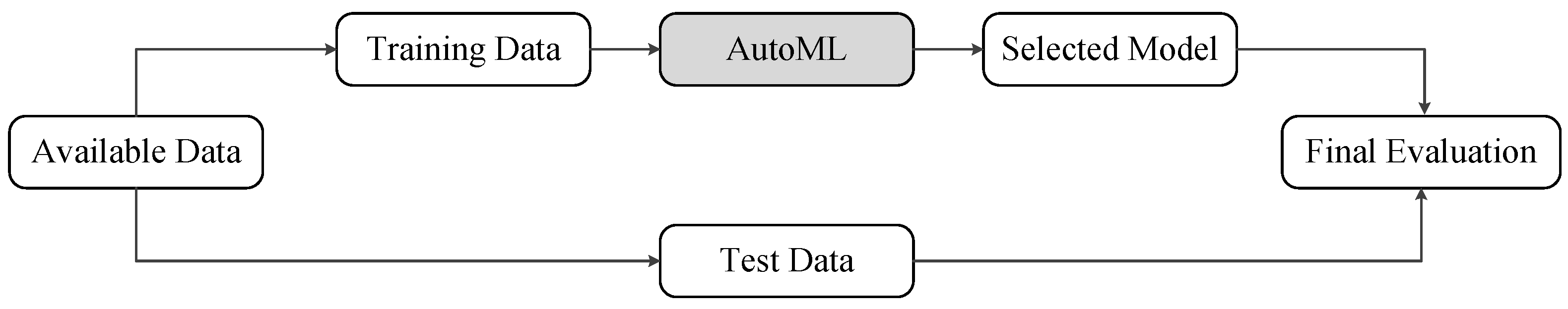
Therefore, AutoML holds great potential to make machine learning and data science more accessible across scientific disciplines to extract patterns and make data-driven decisions. For example, AutoML has been deployed in a wide array of applications, such as image-based plant phenotyping [48], fault severity diagnosis in industrial processes [49], reducing manufacturing costs [50], analyzing biological data [51], and predicting the casualty rate and economic loss induced by earthquakes [52]. Despite the recent progress in this area, we would like to highlight the proper way to evaluate the effectiveness of AutoML techniques. After finalizing a learning method and its hyperparameters using AutoML, one should evaluate its performance on a test or hold-out data set to report its generalization error. This additional step allows us to decouple the model selection process and model assessment, reflecting the “true” performance of the selected model or surrogate when facing new cases. The overall procedure is depicted in Figure 1 via a flowchart. The training data set will be used along with an AutoML technique to select the final model and its hyperparameters, while the test data will be used to report evaluation metrics on unseen data to measure the generalization error.

Given the above introduction of AutoML, we explain the underlying concepts in more detail. Let $\mathcal{A}=\{A^{\left(1\right)},\dots ,A^{\left(N\right)}\}$ represent a set of N eligible machine learning algorithms. Moreover, each $A^{\left(n\right)}$, $n=1,\dots ,N$, comes with a set of hyperparameter configurations, represented by ${\Lambda }^{\left(n\right)}$. Furthermore, let us assume that the training data in Figure 1, called ${\mathcal{D}}_{\mathrm{train}}$ is split into K cross-validation folds $\{{\mathcal{D}}_{\mathrm{train}}^{\left(1\right)},\dots ,{\mathcal{D}}_{\mathrm{train}}^{\left(K\right)}\}$ and $\{{\mathcal{D}}_{\mathrm{valid}}^{\left(1\right)},\dots ,{\mathcal{D}}_{\mathrm{valid}}^{\left(K\right)}\}$, such that ${\mathcal{D}}_{\mathrm{train}}^{\left(k\right)}={\mathcal{D}}_{\mathrm{train}}\backslash {\mathcal{D}}_{\mathrm{valid}}^{\left(k\right)}$ for $k=1,\dots ,K$. Given a loss function $\mathcal{L}$ that measures the prediction quality, we make the assumption that $\mathcal{L}(A_{\lambda }^{\left(n\right)},{\mathcal{D}}_{\mathrm{train}}^{\left(k\right)},{\mathcal{D}}_{\mathrm{valid}}^{\left(k\right)})$ represents the loss evaluated on the validation data ${\mathcal{D}}_{\mathrm{valid}}^{\left(k\right)}$ using the training data ${\mathcal{D}}_{\mathrm{train}}^{\left(k\right)}$ and the learning method $A^{\left(n\right)}$ with its corresponding hyperparameter choices $\lambda \in {\Lambda }^{\left(n\right)}$. With this notation in place, the main idea behind automated machine learning is to solve the following minimization problem in an efficient and robust manner:

$$\underset{A^{\left(n\right)}\in \mathcal{A},\lambda \in {\Lambda }^{\left(n\right)}}{arg\; min}\frac{1}{K}\sum _{k=1}^K\mathcal{L}(A_{\lambda }^{\left(n\right)},{\mathcal{D}}_{\mathrm{train}}^{\left(k\right)},{\mathcal{D}}_{\mathrm{valid}}^{\left(k\right)})$$

(1)

The solution to the above problem results in finding the best learning method and its hyperparameters, which can be used as a surrogate model to capture the behavior of the desired system as accurately as possible. As mentioned before and depicted in Figure 1, an additional step is to evaluate the performance of the selected model on a hold-out test data set to ensure that the model generalizes well beyond the existing data ${\mathcal{D}}_{\mathrm{train}}$.

Among available AutoML techniques/frameworks, we have decided to use auto-sklearn [53,54] in this paper because of five main reasons. First, auto-sklearn is a Python-based open-source toolkit, which resembles the widely-used scikit-learn machine learning package, also known as sklearn [55]. This means that we can use similar methods such as “fit” and “predict” to train and evaluate models, respectively. Second, during the optimization process, auto-sklearn can automatically create an ensemble of top-performing models, instead of reporting a single model with the highest accuracy. To be more formal, the final solution of auto-sklearn can take the form of ${\sum }_n{\beta }_n{A}_{\lambda }^{\left(n\right)}$, where the weights should satisfy $0\le {\beta }_n\le 1$ and ${\sum }_n{\beta }_n=1$. As a result, the top-performing models will have ${\beta }_n>0$ to contribute to the final surrogate model. It has been shown that ensemble methods provide an efficient way to improve predictive accuracy, e.g., [56], which makes auto-sklearn a very attractive choice. Third, auto-sklearn allows us to solve multi-output problems in which the goal is to predict multiple quantities of interest at the same time. This is an important feature of auto-sklearn because, for the application of seismic design of dams, we have to describe the system’s behavior using various quantities, and training distinct models for each quantity becomes intractable. Currently, PyCaret, which is another popular AutoML framework [57], does not support multi-output regression models, which is a substantial drawback for many applications, including the problem of interest in this paper.

The fourth reason is that auto-sklearn runs within a user-determined time budget, with the default value of one hour. Therefore, the user has the option to spend more or less time depending on the computational requirements and the availability of resources. Finally, the fifth reason is that the search space of auto-sklearn is significantly large and considers various regression models and classifiers from the scikit-learn library. For example, in the most recent version of auto-sklearn 0.15.0 that we use in this paper, the following regression models $\mathcal{A}$ are included in the search space:

• Linear models: minimizing a regularized empirical loss with stochastic gradient descent (SGD), and Bayesian Automatic Relevance Determination (ARD) regression;
• Ensemble models: Adaboost, random forest (and decision trees), extra trees, gradient boosting;
• Probabilistic model: Gaussian process (GP) regression;
• K-nearest neighbor (KNN) and support vector regression (SVR);
• Neural networks: Multilayer perceptron (MLP).

Although we refer interested readers to the sklearn documentation page for more detailed information and updates regarding these models and their implementations, we can immediately see the diversity of the models that are included in solving the above optimization problem. To demonstrate the ease-of-use of auto-sklearn for practitioners without a deep knowledge of machine learning methods, we show relevant code snippets for performing the three main steps involved in our proposed framework in Listing 1: (1) dividing the available data into training and test sets, (2) model selection using ${\mathcal{D}}_{\mathrm{train}}$, and (3) model assessment via ${\mathcal{D}}_{\mathrm{test}}$. To save space, we listed $R^2$ or the coefficient of determination as the only score to measure the quality of predictions, but we will use a broader list of evaluation metrics in our numerical results. As a final point, once auto-sklearn finds the best model according to the search space and the given time budget, we can store/load the surrogate model “automl” to make predictions in the future.

Listing 1. Sample of auto-sklearn code to perform the proposed framework.

3. Design Variables

The feasibility level design of a gravity dam includes the selection of an appropriate cross-section including the material properties for the coupled system that satisfy the design objectives under the applied loads. Figure 2 illustrates a generic gravity dam including the dimensions, material properties, and loading.

3.1. Dam Shape

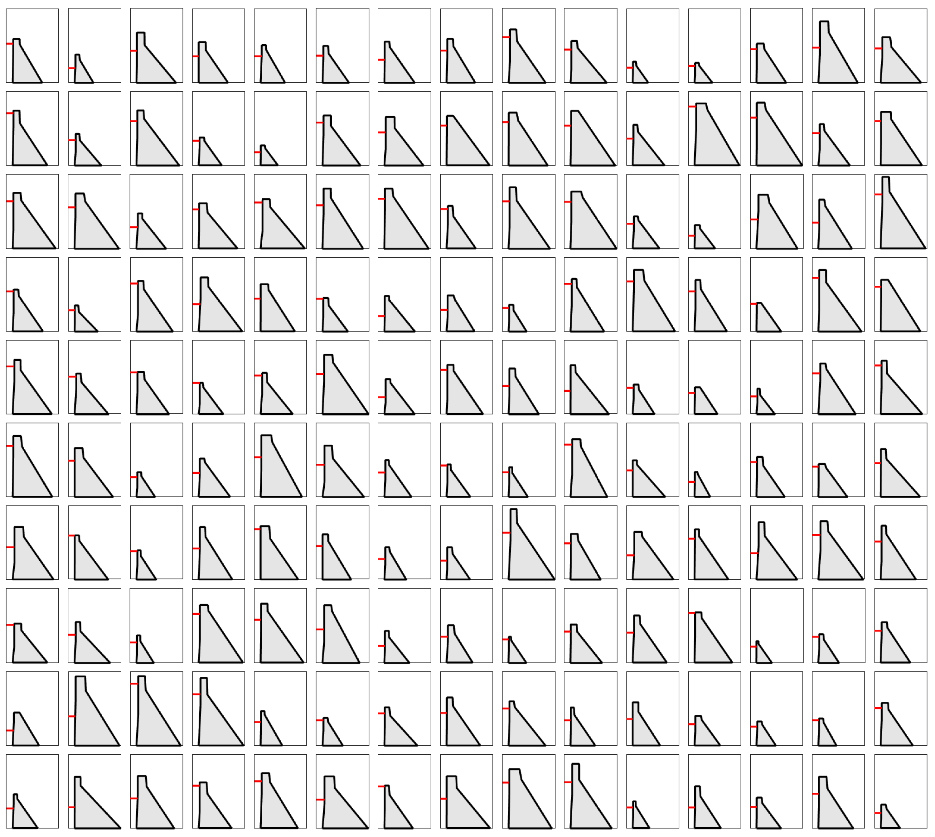
Probably the most important task during seismic design is to select an optimal initial cross-section. Multiple sources offer a cross-section for concrete gravity and arch dams. A large inventory of dams has been studied and a generic dam shape is developed using seven length-related variables as shown in Figure 3 ($L_1$ to $L_7$). All dimensions are a random dependent of the dam base. Furthermore, the reservoir is modeled by assuming a random water level between 50–100% of dam height (corresponding to winter and summer conditions). All the generated dam layouts are consistent with current dam design practices or an existing dam.

• $L_1\in$ (50, 150) m.
• $L_2$ = $L_1\times {\alpha }_1$; ${\alpha }_1\in (0.00,0.05)$⟶$L_2\in$ (0, 7) m.
• $L_3$ = $L_4\times {\alpha }_3$; ${\alpha }_3\in (1.00,1.20)$⟶$L_3\in$ (7, 40) m.
• $L_4$ = $L_1\times {\alpha }_2$; ${\alpha }_2\in (0.12,0.24)$⟶$L_4\in$ (6, 35) m.
• $L_5$ = $L_6\times {\alpha }_5$; ${\alpha }_5\in (0.30,0.70)$⟶$L_6\in$ (20, 140) m.
• $L_6$ = $L_1\times {\alpha }_4$; ${\alpha }_4\in (1.10,1.60)$⟶$L_5\in$ (55, 235) m.
• $L_7$ = $L_5\times {\alpha }_6$; ${\alpha }_6\in (0.75,0.90)$⟶$L_7\in$ (40, 200) m.
• $WL$ = $L_5\times {\alpha }_7$; ${\alpha }_7\in (0.50,1.00)$

3.2. Material Properties

The design of a new dam requires the definition of material properties for finite element simulations. The concrete properties mainly depend on the mix design, and also the availability of the ingredients (e.g., sand, gravel, and cement) near the dam site. The rock properties are typically obtained from geological surveys. However, for feasibility-level design, the exact rock properties might not be available yet. Moreover, the reservoir bottom reflection coefficient, ${\alpha }_w$, is needed which simulates the impact of bottom sediments and alluvium. For new dams, ${\alpha }_w>0.9$ is typically used. However, to account for long terms effects, smaller values should be used. Seven properties are assumed to be unknown during the design process. Each one covers a wide range of possible values.

Concrete modulus of elasticity $E_c\in [15,45]$ GPa, concrete Poisson’s ratio ${\nu }_c=0.2$ (fixed), concrete mass density ${\rho }_c\in [2200,2600]$ kg/m${}^3$, concrete hysteretic damping ${\eta }_c\in [0.02,0.10]$, rock modulus of elasticity $E_r\in [15,45]$ GPa, rock Poisson’s ratio ${\nu }_r=0.33$ (fixed), rock mass density ${\rho }_r\in [2200,2800]$ kg/m${}^3$, rock hysteretic damping ${\eta }_r\in [0.02,0.08]$, and the reservoir bottom wave reflection coefficient ${\alpha }_w\in [0.5,0.9]$. All material properties are sampled based on a truncated normal distribution using the Latin Hypercube sampling technique. No correlation is assumed among these variables. Figure 4 shows the distribution of the material properties used for surrogate modeling. Concrete compressive strength, $f_c^{\prime }$, is not directly used in finite element analyses; however, the results of linear elastic simulations should be compared to tensile ($f_t^{\prime }\approx 0.1f_c^{\prime }$) and compressive strength to ensure the demand does not exceed the capacity.

3.3. Loads

The inputs to the finite element model include both the ground motion records and the water pressure (both hydrostatic and hydrodynamic components). As discussed earlier, the water level is assumed to be 50–100% of the dam height. Subsequently, the corresponding hydrostatic and hydrodynamic pressures are automatically computed and applied by the software. For the seismic simulations, a large database of 160 ground motions is selected worldwide to consider the aleatory uncertainty. While the current practice in earthquake engineering is to select the ground motion records based on the seismic hazard characteristics of the dam site, a random record selection process is used in this paper to generate the surrogate model (later we will show the application of ground motion selection and scaling for a particular dam site). A random ground motion selection is especially useful because none of the generic dams in this paper are associated with a specific site/location. Moreover, variation of the geometry and material properties in the generic models changes the vibration characteristics of the structures (e.g., fundamental period). Thus, ground motion selection and scaling methods such as spectral matching are not practical methods.

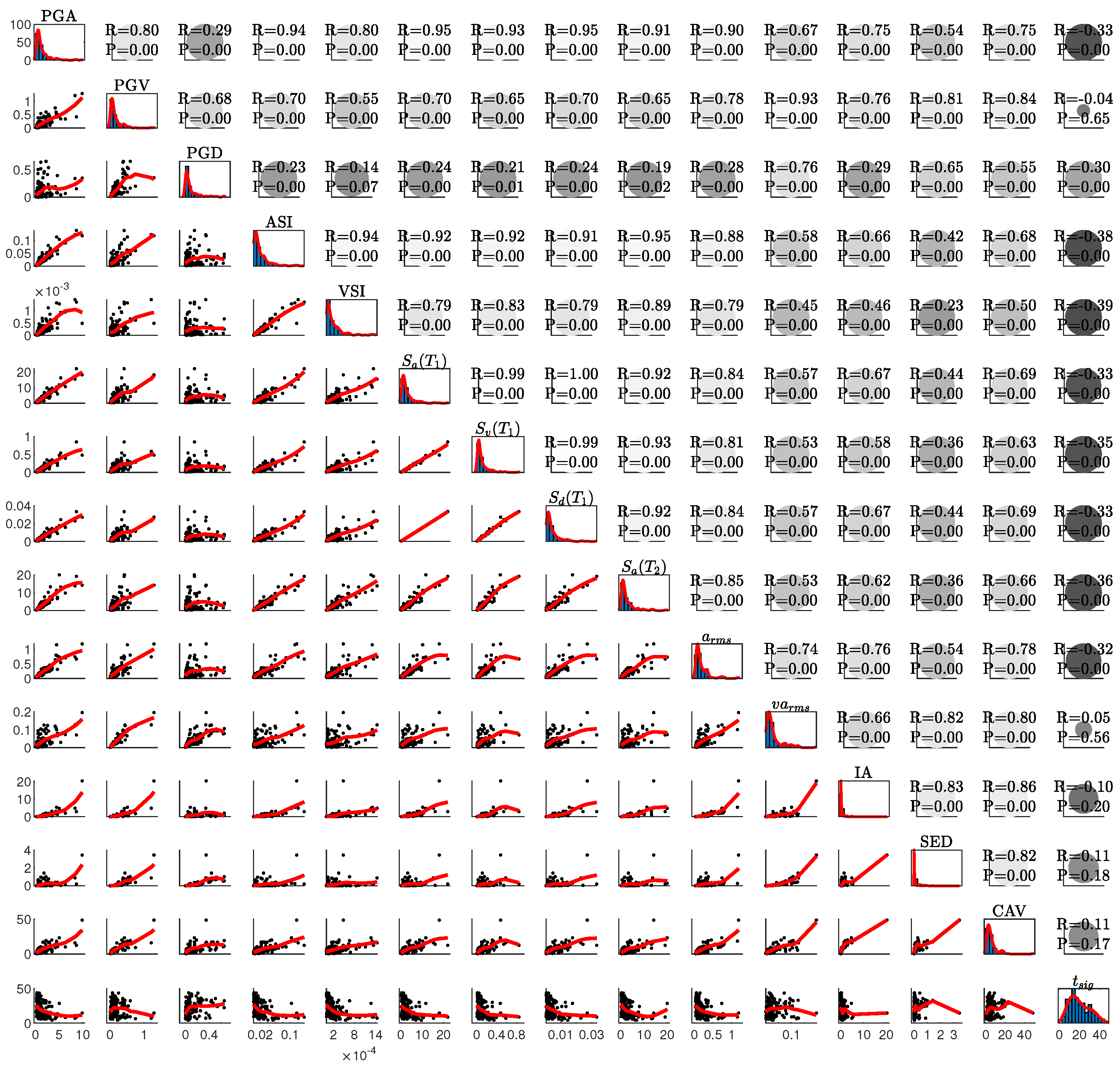
Since a ground motion record has a stochastic nature, one cannot directly use it for classical machine learning regression (unless a time series regression is used which is a complex task). Therefore, it is efficient to extract several meta-features. It is possible to distinguish the ground motion records based on their unique characteristics. A wide range of time-, frequency-, spectral- and intensity-dependent intensity measure (IM) parameters are summarized in

Table 1. A list of ground motion IMs [58].

No.	Description of IM	Symbol	Mathematical Model
1	Peak ground acceleration	$PGA$	$max\left(\left|\ddot{u}\left(t\right)\right|\right)$
2	Peak ground velocity	$PGV$	$max\left(\left|\dot{u}\left(t\right)\right|\right)$
3	Peak ground displacement	$PGD$	$max\left(\left|u\left(t\right)\right|\right)$
4	Acceleration spectrum intensity	$ASI$	${\int }_{0.1}^{0.5}{S}_a\left(T,\xi \right)dT$
5	Velocity spectrum intensity	$VSI$	${\int }_{0.1}^{2.5}{S}_v\left(T,\xi \right)dT$
6	First-mode spectral acceleration	$S_a\left(T_1\right)$	$S_a(T_1,\xi )$
7	First-mode spectral velocity	$S_v\left(T_1\right)$	$S_v(T_1,\xi )$
8	First-mode spectral displacement	$S_d\left(T_1\right)$	$S_d(T_1,\xi )$
9	First-mode spectral acceleration	$S_a\left(T_2\right)$	$S_a(T_2,\xi )$
10	Root-mean-square of acceleration	$a_{RMS}$	${\left(\frac{1}{t_{tot}}{\int }_0^{t_{tot}}{\left(\ddot{u}\left(t\right)\right)}^{2}dt\right)}^{1/2}$
11	Root-mean-square of velocity	$v_{RMS}$	${\left(\frac{1}{t_{tot}}{\int }_0^{t_{tot}}{\left(\dot{u}\left(t\right)\right)}^{2}dt\right)}^{1/2}$
12	Arias intensity	$I_A$	$\frac{\pi }{2g}{\int }_0^{t_{tot}}{\left(\ddot{u}\left(t\right)\right)}^{2}dt$
13	Specific energy density	$SED$	${\int }_0^{t_{tot}}{\left(\dot{u}\left(t\right)\right)}^{2}dt$
14	Cumulative absolute velocity	$CAV$	${\int }_0^{t_{tot}}\left|\ddot{u}\left(t\right)\right|dt$
15	Significant duration	$t_{sig}$	$t_{0.95I_A}-t_{0.05I_A}$

Note: $\ddot{u}\left(t\right)$, $\dot{u}\left(t\right)$ and $u\left(t\right)$ are acceleration, velocity and displacement time histories, respectively.

[58,59]. For each single ground motion signal, fifteen IM parameters are extracted. Figure 5 shows the correlation among fifteen IM parameters for a pilot dam (i.e., a dam that all its shape and material parameters are close to the median of the design space). The lower triangular cells show the one-by-one correlation between 160 ground motion records. The diagonal cells are the histogram of data points. The upper triangular cells are the correlation in terms of Spearman’s linear correlation coefficient (R) and p-values for testing the hypothesis of no correlation against the alternative hypothesis of a nonzero correlation (P). As seen, the significant duration, $t_{sig}$, has the lowest correlation with other IMs, while the first-mode spectral values have the highest correlation with other IMs.

4. Data Structure

So far, all the design variables including the geometry parameters, material properties, and loading have been discussed. In this section, the finite element software is introduced, and the data structure is explained.

4.1. Software

The finite element code EAGD [60] is used for dynamic analyses, where the foundation rock is idealized as a homogeneous, isotropic, viscoelastic half-plane. A two-dimensional model is developed including 480 elements which is reasonable for linear elastic systems. The dam-foundation interaction effects are included by adding the dynamic stiffness matrix for the rock region in the dam’s equation of motion. This frequency-dependent matrix is defined with respect to the degree of freedom of the nodal points at the dam base [61]. The reservoir water is idealized by a fluid domain of constant depth and infinite length in the upstream direction. The dissipation of hydrodynamic pressure waves by the reservoir bottom materials is accounted for by applying a boundary condition that partially absorbs the incident waves. The system is analyzed based on the following load cases: dam self-weight, water pressure, and the free-field horizontal component of the earthquake ground motion.

4.2. Input-Output Coverage

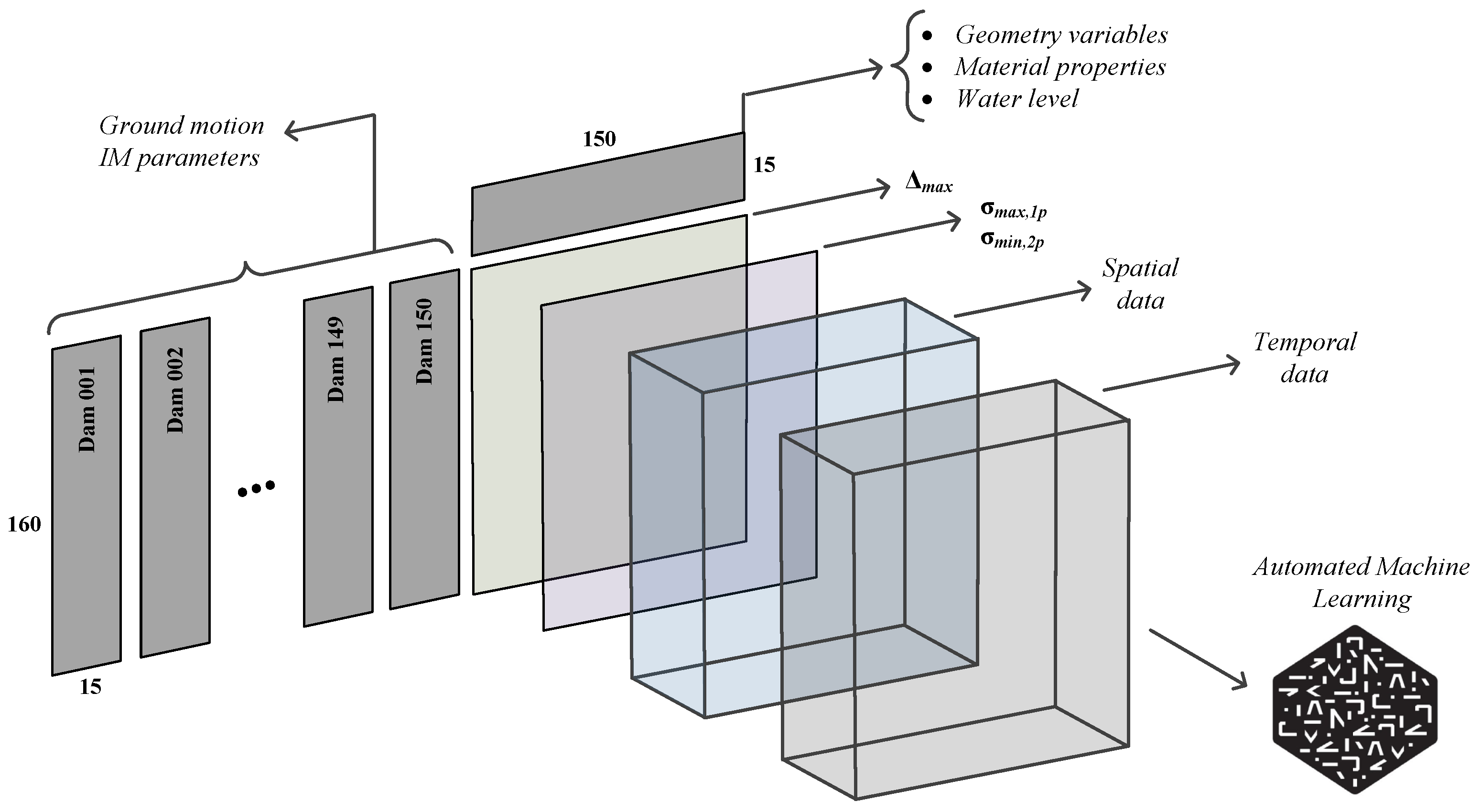
Matlab [62] is paired with EAGD to automate the finite element simulations. A total of 24,000 simulations have been conducted which cover a wide range of dam shapes, material properties, and ground motions. Figure 6 shows the data structure. Two side matrices of $160\times 15\times 150$ and $15\times 150$ are used as inputs in AutoML. The former one is a 3D matrix that identifies the characteristics of the ground motion record. One may note that some of the IM parameters depend on the vibration period of the dam (e.g., $S_a\left(T_1\right)$), and thus, this side matrix is three-dimensional and not two-dimensional. On the other hand, the side matrix which defines the geometry, material, and water level is a two-dimensional matrix as it does not depend on the applied seismic load.

Within the probabilistic simulation framework, and after completing any single finite element analysis, the results are post-processed, and the required information is extracted. Data are stored in the form of a 2D matrix (for scalar quantities) and a 3D matrix (for spatial and temporal quantities).

• Scalar quantities cover the maximum (or minimum) response of the dam at a particular location and the entire duration of the applied ground motion. For example, maximum crest displacement shows the “global” behavior of the dam under the applied motion. Similarly, the maximum first principal stress at the dam heel is a “local” metric that presents the onset of cracking (if exceeds the tensile strength). Other peaks (i.e., maximum or minimum) response quantities can be extracted from displacement, stress, and strain results.
• Vector quantities cover the responses over time, or they present the spatial distribution of the response parameters. Cumulative inelastic duration (CID) shows the time intervals in which the stress at a particular location exceeds the tensile strength. The overstressed area (OA) illustrates the spatial distribution of regions within the dam body where the tensile strength exceeds the tensile strength (or a multiplayer of it).

While it is possible to use as many as output parameters in developing a surrogate model, for any practical implementation, a total of ten response quantities are considered in this paper. They are:

• Out1: maximum horizontal crest displacement, ${\Delta }_{max}$
• Out2: maximum first principal stress at heel, ${\sigma }_{p1,max}^{heel}$
• Out3: maximum first principal stress at upstream face 5% from the heel, ${\sigma }_{p1,max}^{UP5\%}$
• Out4: maximum first principal stress at toe, ${\sigma }_{p1,max}^{toe}$
• Out5: minimum third principal stress at the heel, ${\sigma }_{p2,min}^{heel}$
• Out6: minimum third principal stress at the toe, ${\sigma }_{p2,min}^{toe}$
• Out7: CID for demand capacity ratio exceeds one at the heel, $CI{D}_{DCR=1}^{heel}$
• Out8: CID for demand capacity ratio exceeds two at the heel, $CI{D}_{DCR=2}^{heel}$
• Out9: Overstressed area for demand capacity ratio exceeds one at the heel, $O{A}_{DCR=1}^{heel}$
• Out10: Overstressed area for demand capacity ratio exceeds two at the heel, $O{A}_{DCR=2}^{heel}$

5. Results: Surrogate Model

In this section, we examine the efficacy of auto-sklearn, explained in Section 2, for developing accurate machine learning-based surrogate models mapping the design variables to the quantities of interests (QoI). Specifically, we consider three scenarios that involve predicting: (1) Out2, i.e., single output, (2) outputs 1 through 6, and (3) all 10 outputs discussed in the previous section. The main intention behind this analysis is to better understand the tradeoff between the number of outputs and the quality of the final surrogate models when using AutoML techniques. We hypothesize that the increase in the number of outputs makes it more challenging to find a model (and its corresponding hyperparameters) that performs well across all the desired outputs. Before stating our results, note that the studied outputs fall within substantially different ranges. Thus, it makes sense to use a linear transformation technique for each output individually such that all values of a desired quantity of interest will be transformed into the range $[0,1]$. That is, the minimum and maximum values of the transformed output will be 0 and 1, respectively. To this end, we use the “MinMaxScaler” method from sklearn, where the transformation is given by $(y-min)/(max-min)$ for each output value y.

For all experiments, we use three evaluation metrics that are specifically designed for regression problems. The first one is $R^2$ or the coefficient of determination, which is defined as follows for a set of n finite element results $y_1,\dots ,y_n$ and their predicted values obtained by a machine learning model ${\widehat{y}}_1,\dots ,{\widehat{y}}_n$:

$$R^2(y,\widehat{y})=1-\frac{{\sum }_{i=1}^n{(y_i-{\widehat{y}}_i)}^2}{{\sum }_{i=1}^n{(y_i-\overline{y})}^2},$$

(2)

where $\overline{y}=\frac{1}{n}{\sum }_{i=1}^n{y}_i$ is the sample mean or average. Therefore, the best possible score is 1 when $y_i={\widehat{y}}_i$ for all cases, and the result is 0 when all the predicted values are equal to the sample mean $\overline{y}$, which means that the machine learning model has not learned any patterns. Therefore, $R^2$ values closer to 1 indicate a more accurate machine learning-based surrogate model. The two other evaluation metrics are Root Mean Square Error (RMSE) and Mean Absolute Error (MAE). We can compute these two metrics as follows:

$$\begin{array}{c}\hfill \mathrm{RMSE}(y,\widehat{y})={\left(\frac{1}{n}\sum _{i=1}^n{(y_i-{\widehat{y}}_i)}^2\right)}^{1/2}\end{array}$$

(3)

$$\begin{array}{c}\hfill \mathrm{MAE}(y,\widehat{y})=\frac{1}{n}\sum _{i=1}^n|y_i-{\widehat{y}}_i|.\end{array}$$

(4)

Based on these formulas, when $y_i={\widehat{y}}_i$ for all cases, the return values are zeros, and, overall, values closer to 0 indicate more accurate machine learning or surrogate models.

5.1. Scenario 1: Single Output

In the first scenario, we just consider Out2 (i.e., maximum principal stress at the heel) and use the default time limit of one hour when using auto-sklearn for model selection (we fix the time limit throughout this section).

Table 2. The result of model selection performed by auto-sklearn when considering a single output (Scenario 1).

Rank	Ensemble Weight	Type	Duration
1	$0.16$	Gradient Boosting	$24.10$
2	$0.04$	Gradient Boosting	$3.85$
3	$0.14$	Gradient Boosting	$11.88$
4	$0.24$	ARD Regression	$103.09$
5	$0.06$	Gradient Boosting	$11.311$
6	$0.12$	Gradient Boosting	$3.21$
7	$0.06$	Gradient Boosting	$11.13$
8	$0.10$	Gradient Boosting	$8.95$
9	$0.06$	Gradient Boosting	$147.51$
10	$0.02$	ARD Regression	$1.65$

reports the final result, including the types of machine learning models used in the ensemble and their corresponding weights ${\beta }_n$ as well as the length of time the model was optimized for (called duration). To interpret this table, note that the rank of each model is based on the calculated value of the loss function that we discussed in Section 2; Rank 1 has the lowest value of the loss. In terms of the ensemble method selected by auto-sklearn, as expected, we can confirm that ${\sum }_n{\beta }_n=1$. Furthermore, we notice that the final model consists of two main types of machine learning models: Gradient Boosting and ARD Regression. Gradient Boosting is a boosting-like algorithm for regression that combines weak learners and the main difference between the models listed in the table is related to critical hyperparameters, such as the maximum depth of the tree and the minimum number of samples required to split an internal node [63]. On the other hand, the most influential model in the ensemble according to the assigned weight is ARD Regression, which can be viewed as a Bayesian extension of linear regression, where the parameters of the regression model are assumed to be in Gaussian distributions. Due to its probabilistic nature, training such models can be time-consuming, as evident from the duration column of Table 2.

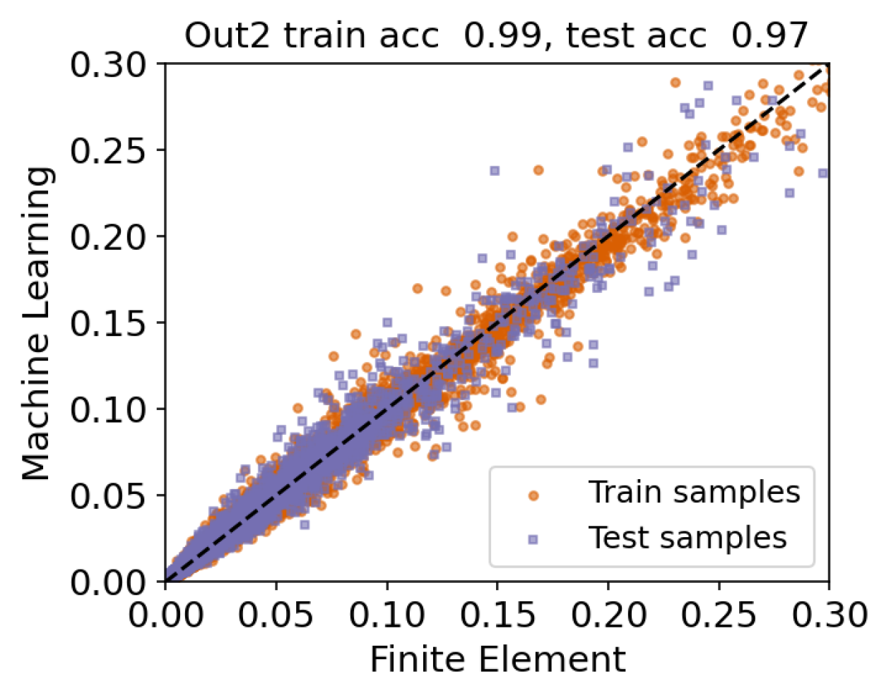
Next, we present a parity plot to better understand the performance of the final model using both training and test data sets. This step is crucial because we should show that the final model is not suffering from overfitting, which is a common problem when the selected machine learning model is too complex for the problem at hand. Particularly, Figure 7 plots true values of the quantity of interest obtained via our finite element model versus predicted values produced by the machine learning model that auto-sklearn selected. The reason that we focus on the range $[0,0.3]$, instead of $[0,1]$, is that the majority of scaled output values fall within this range. Hence, this allows us to visualize the behavior of the surrogate model more closely in this interesting regime. However, we use the entire data set to report evaluation metrics. In the title of this figure, the accuracy score refers to $R^2$ or the coefficient of determinations, and the best possible score is 1. Therefore, we corroborate that the trained surrogate model performs well on both training and test data sets. In addition, we evaluated the performance of this model on the test data using the other discussed metrics: $\mathrm{RMSE}=0.008$ and $\mathrm{MAE}=0.004$, showing the reasonable performance of the final surrogate model.

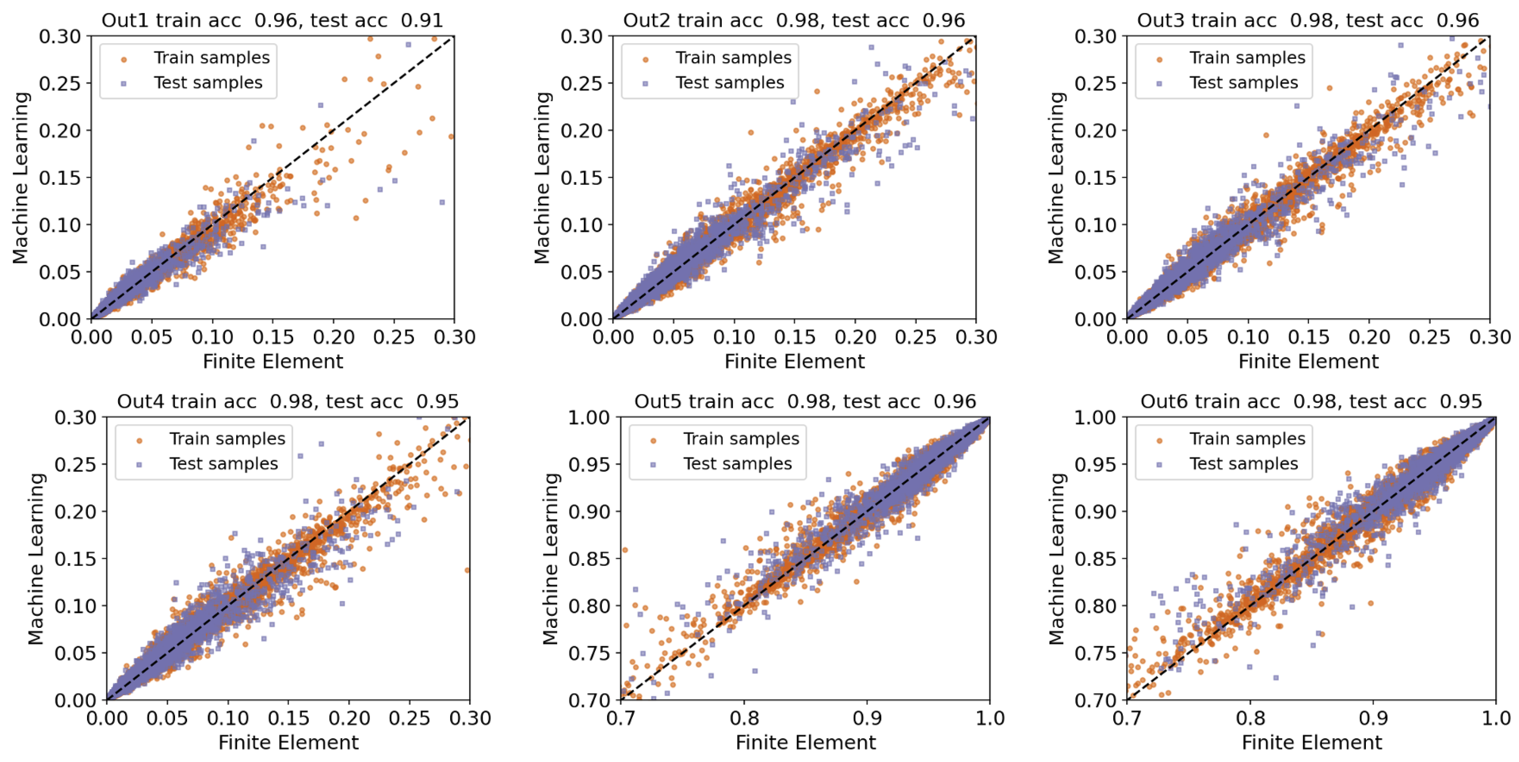
5.2. Scenario 2: Multi-Output, Out1 through Out6

In the second scenario, we consider a multi-output setting, where the objective is to develop a surrogate model to predict six quantities of interest: Out1 through Out6. Similar to the previous experiment, we report the anatomy of the final model, including ranks, ensemble weights/models, and duration, in

Table 3. The result of model selection performed by auto-sklearn when considering six outputs (Scenario 2).

Rank	Ensemble Weight	Type	Duration
1	$0.84$	Extra Trees	$176.97$
2	$0.06$	Random Forest	$132.60$
3	$0.10$	K-Nearest Neighbor	$19.53$

. Note that the final model primarily consists of tree-based machine learning models. In fact, Extra Trees and Random Forests are similar in the sense that they both build multiple trees and split nodes using random subsets of features. Therefore, their main goal is to improve the predictive accuracy and control overfitting by constructing ensemble methods. However, as apparent in the table, such methods are computationally expensive. On the other hand, K-Nearest Neighbor methods are much faster when working with data sets consisting of a few thousand data points, which is the case in our study. The number of nearest neighbors, which is the most important hyperparameter, is set to 17 in this example.

Moreover, we provide parity plots in Figure 8, where each subfigure represents actual vs. predicted values for both training and test sets accompanied by $R^2$ values. Similar to the previous scenario, we focus on the range $[0,0.3]$ (except for Out5 and Out6) because most output values fall within this range. However, Out5 and Out6 take on negative values, and using the transformation technique that we discussed earlier in this section, the majority of data points that have low absolute values fall within $[0.7,1]$. This is because negative numbers get smaller as their magnitude increases.

To interpret the reported results in Figure 8, note that Out2 is shared between scenarios 1 and 2, and that the performance of the obtained surrogate model in the second case is slightly worse than the one produced in the first scenario. This is consistent with our hypothesis because the second case study aims to find a model that performs well across all six outputs, instead of a single output. Despite the minor accuracy reduction, we believe that the surrogate model in this scenario is more useful because of predicting multiple outputs at the same time, while the reported $R^2$ values are consistently above $0.9$ across all the desired quantities of interest.

In addition,

Table 4. Evaluating the performance of the trained surrogate model using six outputs: Out1 through Out6.

Output	${\mathit{R}}^2$	RMSE	MAE
Out1	$0.912$	$0.007$	$0.002$
Out2	$0.958$	$0.009$	$0.004$
Out3	$0.956$	$0.009$	$0.004$
Out4	$0.948$	$0.010$	$0.005$
Out5	$0.958$	$0.009$	$0.004$
Out6	$0.947$	$0.010$	$0.005$
Overall	$0.947$	$0.009$	$0.004$

reports the performance of the machine learning-based surrogate model on the testing data using three metrics. Based on these results, we conclude that the overall performance of our model is satisfactory. RMSE and MAE values are less than $0.01$ because the transformed output values are distributed in the range $[0,1]$. Moreover, the overall $R^2$ value is about $0.95$, meaning that the model has learned useful input-output patterns from the training data set.

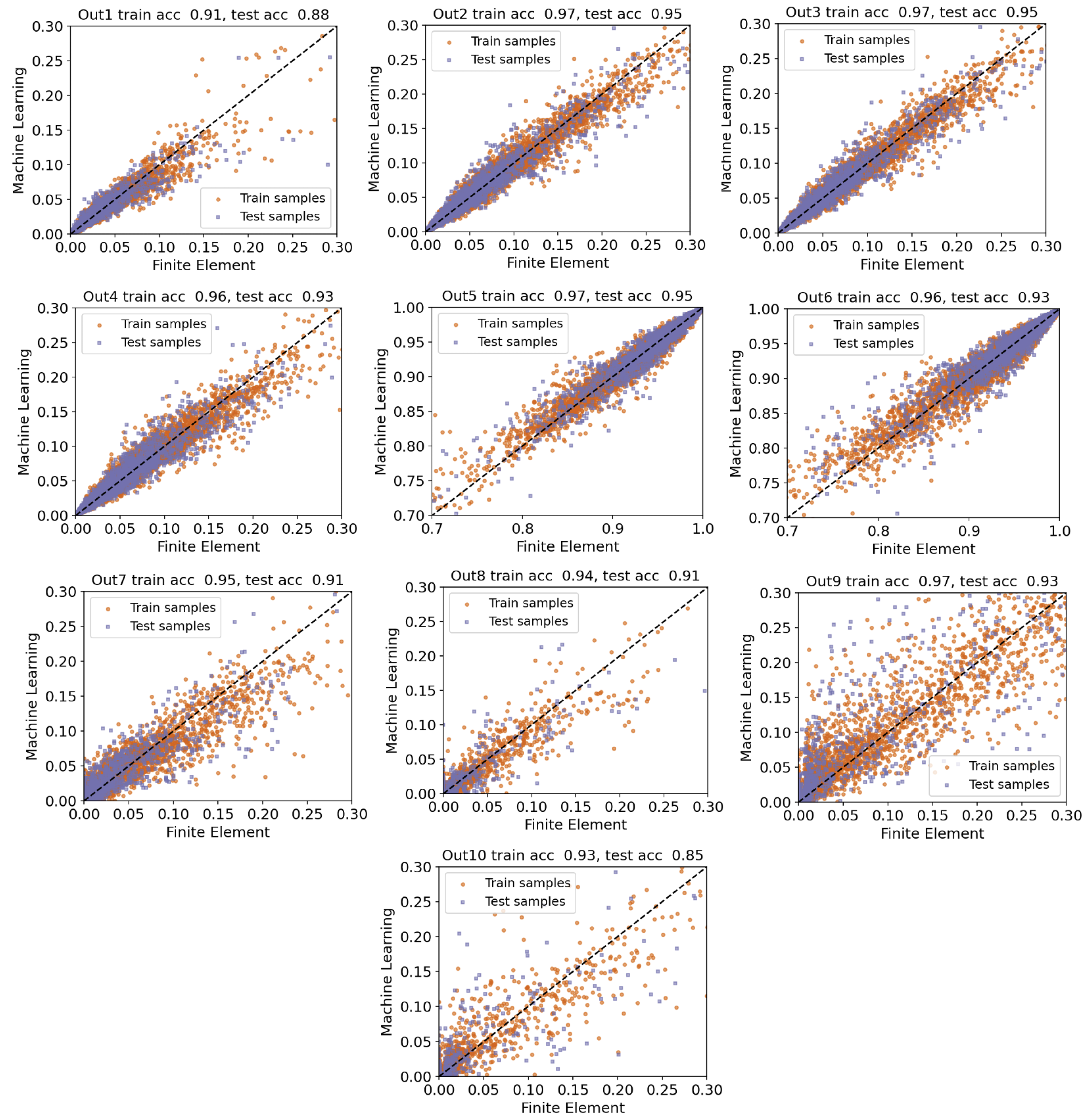
5.3. Scenario 3: Multi-Output, Out1 through Out10

In this section, we extend our previous analysis to account for the 10 outputs explained in Section 4.

Table 5. The result of model selection performed by auto-sklearn when considering all ten outputs (Scenario 3).

Rank	Ensemble Weight	Type	Duration
1	$0.08$	Decision Tree	$1.88$
2	$0.04$	Decision Tree	$158.13$
3	$0.22$	Decision Tree	$161.25$
4	$0.04$	Decision Tree	$6.22$
5	$0.16$	Decision Tree	$7.37$
6	$0.06$	Decision Tree	$1.22$
7	$0.06$	Decision Tree	$160.86$
8	$0.20$	Decision Tree	$101.23$
9	$0.02$	Decision Tree	$1.7$
10	$0.04$	Decision Tree	$69.75$
11	$0.02$	K-Nearest Neighbor	$18.94$
12	$0.06$	K-Nearest Neighbor	$1.31$

presents the structure of the final ensemble method identified by using auto-sklearn. This model mainly contains Decision Trees and the K-Nearest Neighbor regression models. From the computational standpoint, optimizing the Decision Tree model is typically more time-consuming than training the K-Nearest Neighbor model. However, from the predictive accuracy viewpoint, Decision Trees are popular because they learn simple decision rules from the available data to approximate a wide range of linear and nonlinear functions, which is helpful when considering various input-output mappings. By carefully reviewing the selected hyperparameters, we noticed that the main difference between the chosen Decision Trees is the minimum number of samples required to split an internal node in the tree (ranging from 3 to 19). On the other hand, the number of nearest neighbors for the two selected models is set to 4 and 17. As a final point, it is interesting to observe that the K-Nearest Neighbor regression model with 17 neighbors was also found in the previous scenario, where we considered 6 outputs.

Furthermore, Figure 9 presents parity plots for the resulting surrogate model when considering all ten outputs, showing actual values obtained by the finite element analysis on the horizontal axis and the corresponding predicted values by the surrogate model on the vertical axis. Comparing the first six outputs with the results from the previous case study, we again notice an insignificant reduction in the predictive accuracy measured by the $R^2$ score. This reduction is reasonable given that the new surrogate model should predict a larger number of outputs compared to the previous case. However, except for Out1 and Out10, the accuracy score exceeds $0.9$. To have a more detailed analysis of this surrogate model, we report two other additional metrics (RMSE and MAE) in

Table 6. Evaluating the performance of the trained surrogate model using 10 outputs: Out1 through Out10.

Output	${\mathit{R}}^2$	RMSE	MAE
Out1	$0.884$	$0.008$	$0.003$
Out2	$0.946$	$0.010$	$0.005$
Out3	$0.947$	$0.010$	$0.005$
Out4	$0.933$	$0.011$	$0.005$
Out5	$0.950$	$0.009$	$0.005$
Out6	$0.927$	$0.012$	$0.006$
Out7	$0.912$	$0.013$	$0.004$
Out8	$0.909$	$0.009$	$0.001$
Out9	$0.926$	$0.032$	$0.010$
Out10	$0.854$	$0.016$	$0.003$
Overall	$0.919$	$0.013$	$0.005$

. Based on these results, the overall $R^2$ score is above $0.9$ and the final RMSE and MAE values are on par with the previous case that we just considered six outputs. Therefore, based on our analysis, we conclude that auto-sklearn is capable of performing model selection in challenging scenarios involving the prediction of multiple quantities of interest at the same time. As a result, auto-sklearn provides an easy-to-use framework for non-experts in machine learning and practitioners because of eliminating the need to develop multiple independent surrogate models for individual outputs.

6. Results: Dam Design Engine

Having multiple surrogate models from Section 5, this section discusses the implementation of those in a context of a design engine. In general, a surrogate model aims to estimate the structural responses as a function of dam shape, material parameters, water level, and applied ground motion:

$$\mathbf{QoI}=g\left(\underset{Material}{\underbrace{{\mathrm{Mat}}_1,\cdots ,{\mathrm{Mat}}_7}},\underset{Shape}{\underbrace{L_1,\cdots ,L_7}},\underset{Water}{\underbrace{L_w}},\underset{Seismic}{\underbrace{{\mathrm{IM}}_1,\cdots ,{\mathrm{IM}}_{15}}}\right)$$

(5)

where the input parameters take a range of values for each of the 30 input parameters, and $\mathbf{QoI}$ is a matrix of outputs (i.e., quantities of interests).

In any practical seismic dam design process, the seismic hazard scenario for which the dam should be designed is known (from probabilistic or deterministic seismic hazard analysis—PSHA/DSHA [64,65]) and is provided to the structural team by a seismologist. Moreover, the basic material properties are also available with good confidence. The foundation rock properties are determined by geologists including the profile of shear wave velocity, mass density, elasticity, permeability, shear strength, etc. [66]. The mechanical properties in concrete are governed by mix design and can be assumed to be known for the feasibility level design [67,68]. Finally, some of the shape parameters are known with good confidence at the feasibility level of design. For example, the total dam height is usually provided to the engineer by the project manager (with inputs from the dam owner, and hydrology team). Therefore, an inverse analysis can be performed on the pre-generated surrogate model using the known variables (specified with an asterisk in the following equation) to estimate the unknown ones:

$$\underset{Unknownvariables}{\underbrace{\left[{\mathrm{Mat}}_{\sim i},L_{\sim j}\right]}}=g^{-1}\left(\underset{Water}{\underbrace{L_w^{*}}},\underset{Seismic}{\underbrace{{\mathrm{IM}}_1^{*},\cdots ,{\mathrm{IM}}_{15}^{*}}},\underset{Material}{\underbrace{{\mathrm{Mat}}_i^{*}}},\underset{Shape}{\underbrace{L_j^{*}}},{\mathbf{QoI}}^{*}({\sigma }_{p1,max}^{heel},{\Delta }_{max},\cdots )\right)$$

(6)

where index i and j are known material and shape variables, and $\sim i$ and $\sim j$ are the remaining unknown variables. ${\mathbf{QoI}}^{*}$ are a series of target responses for the design earthquake.

To explain the technical aspects of the inverse analysis, let us assume that the final surrogate model obtained by auto-sklearn (or other AutoML techniques) takes the form of $g({\theta }_i,{\theta }_j,{\theta }_{\sim i},{\theta }_{\sim j})$, where ${\theta }_i$ and ${\theta }_j$ represent all known variables that we can treat them as constants and the other two variables are unknown. Here, the goal is to find the “best” choices of ${\theta }_{\sim i},{\theta }_{\sim j}$ such that the value of the function g gets as close as possible to the target response $g^{*}$. There are two main steps involved in solving this problem: (1) defining a search space, i.e., the set of possible values for the unknown variables, and (2) casting an optimization problem. We denote the search space for each variable type by ${\theta }_{\mathrm{material}}$ and ${\theta }_{\mathrm{shape}}$. With this notation in place, the optimization problem takes the following form:

$$\underset{{\theta }_1\in {\theta }_{\mathrm{material}},{\theta }_2\in {\theta }_{\mathrm{shape}}}{arg\; min}|g^{*}-g({\theta }_i,{\theta }_j,{\theta }_1,{\theta }_2)|.$$

(7)

Since the size of the search space is finite, we can find the objective function in the above optimization problem for each feasible solution, and then sort them in ascending order. This means that we will have a “ranked” list of possible solutions for the inverse problem.

Design earthquake and ground motion records for dam projects are typically obtained from two main sources [7]: ICOLD and FEMA. While the detailed discussion on ground motion selection and scaling is beyond the coverage of this paper, some major aspects are clarified [69].

• ICOLD recommendations There are two basic seismic loads for the design of new dams [70]: Operating Basis Earthquake (OBE) which represents the seismic intensity level at the dam site for which only minor (easily repairable) damage is acceptable and the dam should remain functional. The OBE corresponds to the return period of 145 years (50% probability of exceedance in 100 years). Safety Evaluation Earthquake (SEE) represents the seismic intensity level at the dam site for which a dam must be able to resist without the uncontrolled release of the reservoir water. The SEE ground motion can be obtained from a probabilistic and/or deterministic seismic hazard analysis. For large and high consequence dams, SEE is defined as (a) Maximum Credible Earthquake (MCE) from DSHA where the parameters should be estimated at the 84th percentile level, (b) Maximum Design Earthquake (MDE) from PSHA corresponding to return period of 10,000 years (1% probability of exceedance in 100 years) [71,72].
• FEMA recommendations Time-based performance assessment evaluates a dam’s performance over a period considering all earthquakes that may occur in that period, and the probability that each will occur [73]. This procedure follows the following main steps: (a) generate a seismic hazard curve, i.e., $\lambda$ vs. $S_a\left(T_1\right)$, (b) compute seismic intensity range and split it into $N_i$ equal intervals, (c) develop a target response spectrum, $S_a^{trg}\left(T\right)$, for each intensity range, and (d) select and scale suites of $N_{gm}$ ground motions for each spectrum.

Having the scaled ground motions, all the intensity measure parameters listed in Table 1 should be calculated. While the majority of these IMs are structure-independent, some are calculated based on the vibration period of the system (e.g., $S_a\left(T_1\right)$). However, at this stage, the shape (and maybe some of the material properties) are unknown, and thus, direct finite element modeling cannot be used. Instead, a simplified method is used to estimate the initial fundamental period of the dam. The formulation is based on Algorithm 1 originally proposed by [74] by introducing a set of new dynamic compliance coefficients.

Algorithm 1: Estimation of the fundamental period of the coupled system [74,75].

Inputs:$L_w$ [m], $L_6$ [m], $E_c$ [MPa], $E_r$ [MPa], ${\alpha }_w$ Output:$T_{dwf}$ [sec]. 1: procedure 2:     $D_r=\frac{L_w}{L_6}$                                                                                                                                                        ▹ Depth ratio 3:     $T_d=0.38\frac{L_6}{\sqrt{E_c}}$                                                                                      ▹ Fundamental period of a “standard” section 4:     $R_r=f(D_r,E_c,{\alpha }_w)$    ▹ Standard values for the period lengthening ratio due to hydrodynamic [74], Figure 10 5:     $R_f=0.21{\left(E_r\right)}^{-0.75}+0.98$                  ▹ Standard values for the period elongation ratio due to foundation [75] 6:     $T_{dwf}=R_r{R}_f{T}_d$                                                                  ▹ Fundamental period of dam-water-foundation system 7: end procedure

Figure 10. Standard values for the period lengthening ratio due to hydrodynamic effects, $R_r$.

Figure 10. Standard values for the period lengthening ratio due to hydrodynamic effects, $R_r$.

Example of AutoML Seismic Design

In this section, we elaborate on the practical implementation of the design engine for a hypothetical site in the central north United States. The objective is to design a straight concrete gravity dam with a 100 m height. The dam is located in a relatively wide valley. The normal water level is provided to be 95 m. According to the concrete mix design, the concrete modulus of elasticity and mass density are 22 GPa, and 2400 kg/m${}^3$, respectively. The measured shear wave velocity for the top 30 m of rock is about 2250 m/s, and the rock mass density is 2600 kg/m${}^3$. Therefore, the modulus of elasticity of the rock is estimated to be 35 GPa. For the feasibility level design, a 0.06 and 0.04 constant hysteretic damping is assumed for the dam and foundation respectively, which correspond to 3% and 2% of viscous damping for each substructure. The combined damping value for the overall dam-water-foundation system is then larger than damping values measured from field tests on several dams, and it is close to the 90% percentile of the collected data by Chopra [7]. Moreover, the reservoir bottom wave reflection coefficient of 0.9 is used.

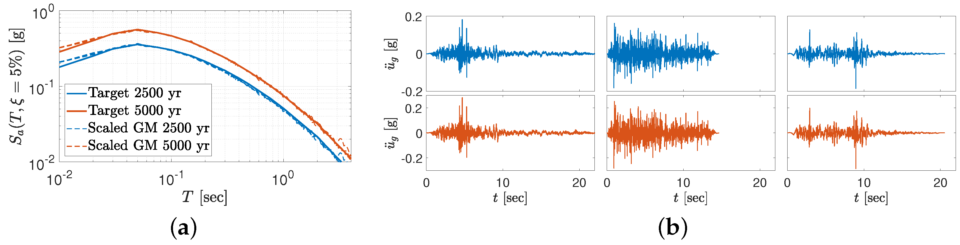
Following a probabilistic seismic hazard analysis (which is beyond the coverage of this paper), two seismic hazard levels with 2500 and 5000 years of the return period (RP) are identified for the dam site (denoted as RP2500 and RP5000). The target and individual response spectra for the scaled records are plotted in Figure 11a. The scaled records are also shown in Figure 11b. While the three-component records are typically scaled based on the target spectra, only a single component is shown for this hypothetical example.

While different objectives can be defined by the design team for the feasibility level design, this example is solely focused on the structural aspects and does not consider the construction cost, as well as risk-informed constraints [13]. This means that the design does not consider the concrete volume used for construction and also the architectural elements. It also does not consider the population at risk in the downstream dam.

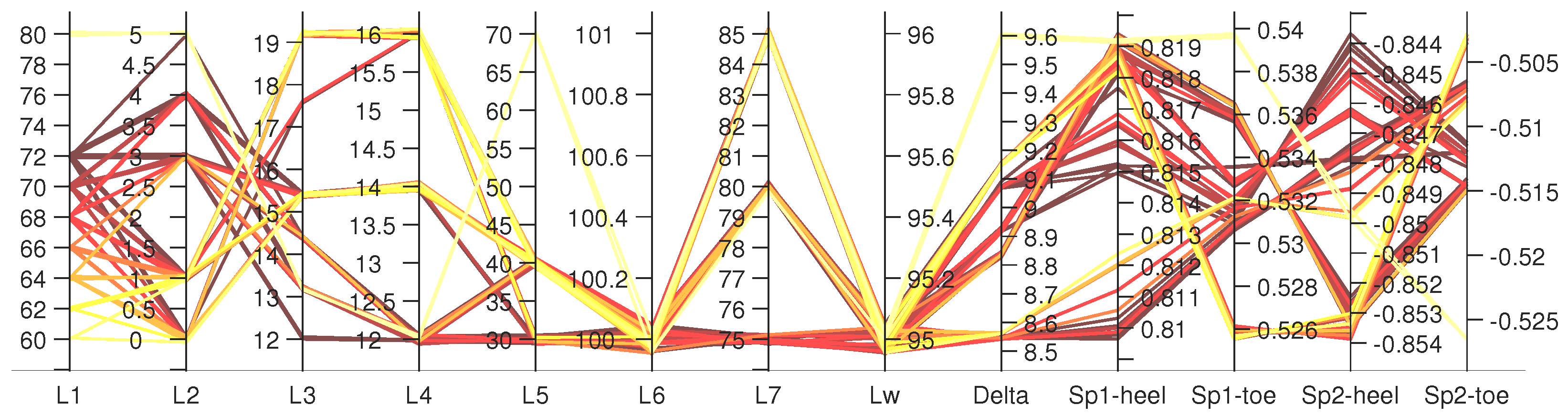
We assume that the maximum dynamic tensile stress at the dam heel should be limited to 0.75 MPa under the 2500 years return period scenario. No other constraint is considered in this example. However, it is possible to add more constraints on stress and/or displacement components. Three ground motion records in Figure 11b are processed, and fifteen IM parameters are extracted as discussed in Table 1. Using engineering judgment, the strongest one (i.e., GM1) is used for design. The most comprehensive surrogate scenario is used (see Section 5.3) which is developed based on ten outputs. An inverse analysis is run, and the top 100 design candidates are identified. Figure 12 illustrates a parallel plot that connects all the design variables for the top 100 candidates to five major outputs (including crest displacement, and maximum/minimum principal stresses at the heel and toe). A large variety of $L_1$ (dam base) values have been included for these top 100 design candidates. The ${\Delta }_{max}$ varies from 8.5 to 9.5 mm which corresponds to 0.0085–0.0095% of dam height. This is close to a threshold value of 0.01% recommended in [76] for gravity dams. The value of ${\sigma }_{p1,max}^{heel}$ is in the [0.81–0.82] MPa range which is close to the threshold value (i.e., 0.75 MPa) previously defined for inverse analysis. The variation in the other three stress quantities is small too.

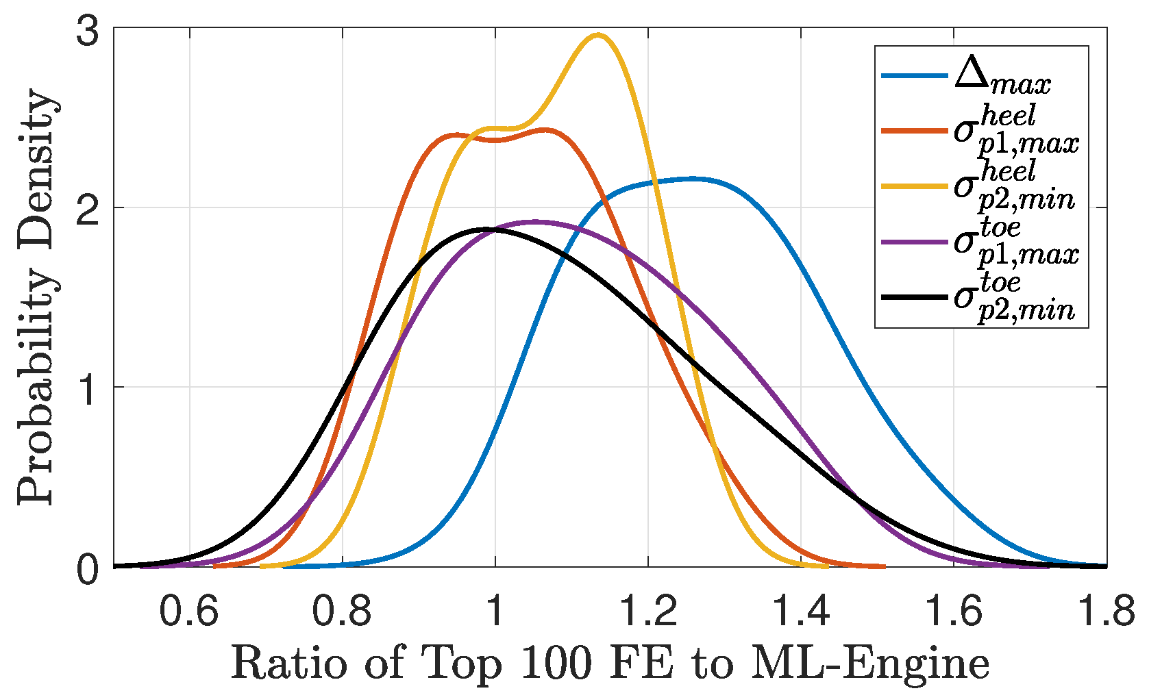
The small variation of displacement and stress responses for the top 100 design candidates, Figure 12, shows that all these models are more or less acceptable from an ML-engine point of view. However, they need to be verified by direct finite element simulations. Therefore, a series of new analyses are conducted using $L_1$ to $L_7$ (and also $L_w$) values in Figure 12 based on GM1 of RP2500, and also the material properties described earlier in this section. The results of direct finite element simulations are collected and compared to those estimated from inverse analysis based on the trained surrogate model. First, the ratio of direct finite element results to the machine learning engine is computed for all top 100 design candidates, as well as five response parameters. Next, a Kernel density function is fitted to each of the five response parameters as shown in Figure 13. As seen, all four stress responses are centered at one showing that the results of inverse analysis fluctuate around the direct finite element simulation. The range of significant ratio variation is 0.7–1.3 (and for compressive stress up to 1.5). This means that despite the similarity of 100 design candidates from the ML point of view, the direct finite element simulation causes considerable differences among them. In the cases of displacement response, a bias is observed between the direct finite element and machine learning engine, as the former tends to 20% more results (on average).

So far, Figure 13 showed the variation of the top 100 design candidates specified by the ML engine and tested by direct finite element simulation. Since only a single design should be selected at the end, we have a closer look at the top three candidates provided by the ML engine. Six (unknown) shape variables for each design are listed here:

• Candidate 1: $L_1=72$ m, $L_2=0$, $L_3=15.4$ m, $L_4=14$ m, $L_5=40$ m, $L_7=75$ m.
• Candidate 2: $L_1=72$ m, $L_2=0$, $L_3=15.4$ m, $L_4=14$ m, $L_5=40$ m, $L_7=85$ m.
• Candidate 3: $L_1=70$ m, $L_2=0$, $L_3=15.4$ m, $L_4=14$ m, $L_5=40$ m, $L_7=80$ m.

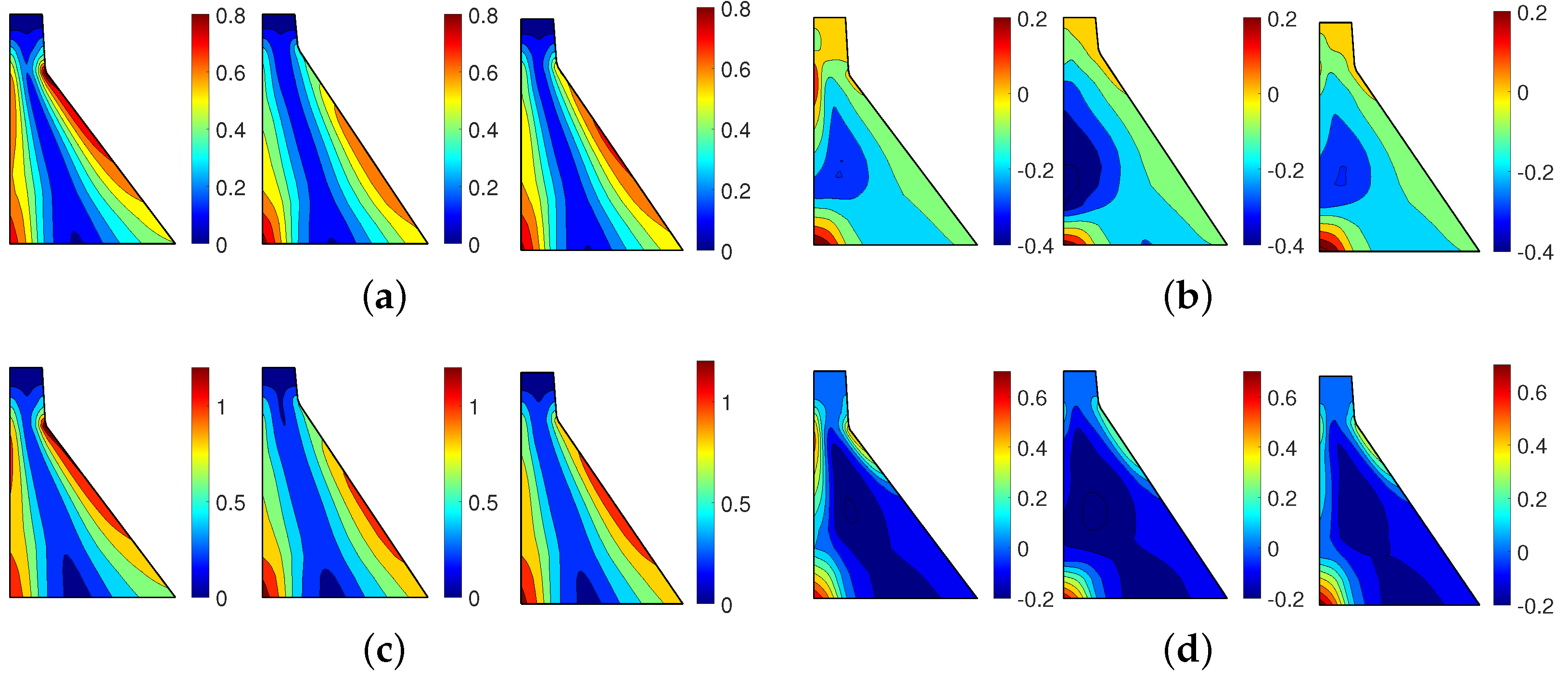
As seen, only $L_1$ and $L_7$ values change for these top three candidates. Figure 14 illustrates the non-concurrent envelop for the first principal stress for top three candidates. Figure 14a presents ${\sigma }_{p1,max}$ only for the dynamic response under RP2500 and GM1. As seen, in all cases ${\sigma }_{p1,max}^{heel}$ is about 0.8 MPa which is close to the predefined value of 0.75 MPa. The locations with high dynamic tensile stress are the dam heel and (to some extent) the downstream face in the vicinity of neck discontinuity. Figure 14b shows the same designs; however, the stress results include the static loads too. In this load combination, the tensile stresses of about 0.2 MPa are only limited to the heel. This is somehow consistent with the traditional design approach that specifies no/limited tension in the dam. While the initial design is based on the RP2500 scenario, the candidate models are further analyzed for RP5000. Figure 14c,d present the results of dynamic only and static+dynamic load combinations for the same three candidates. As seen, the dynamic tensile stresses are increased to about 1.2 MPa in all cases, while the combined tensile stress is about 0.7 MPa at the heel (and for the 1st candidate also around the neck). Depending on the design tensile strength $f_t^{\prime }$, cracking might be expected at the dam-foundation interface which necessitates conducting a nonlinear simulation (beyond the coverage of this paper).

7. Summary

This paper proposed a finite element-based design engine to assist the practitioners in feasibility level layout development for 2D concrete gravity dams under seismic events. The engine includes a large inventory of gravity dam shapes with different material properties for concrete and foundation rock. Such a large inventory has been subjected to different water levels and many ground motion records. The current database covers about 24,000 unique combinations of dam shapes, material properties, water, and earthquake loading. Automated machine learning (AutoML) tool was used to develop a high-fidelity surrogate model. Next, the surrogate model combined with inverse analysis to design new dams that only few of the design variables are known priori.

Using auto-sklearn as an instance of AutoML techniques that are increasing in popularity, we showed that one could build accurate surrogate models capable of predicting multiple quantities of interest simultaneously. Such models typically form an ensemble containing a rich combination of various machine learning methods, such as Bayesian and tree-based methods. Moreover, we presented a principled way to assess the performance of surrogate models obtained by AutoML to understand the generalization error. Future research directions for this task include (1) a comprehensive analysis of the impact of the time budget in auto-sklearn on the quality of surrogate models, and (2) a comparison with other AutoML techniques, including AutoKeras that allows us to restrict our focus on neural network models.

On the design side, the surrogate-assisted inverse analysis showed promising results in early design of concrete gravity dams. The results of inverse analysis was in very good agreement with test data from same surrogate model. However, there were some differences for data beyond those initially used for meta-modeling. This necessitates increasing the database which covers even more ground motion records. We tested the design engine for a single scenario (i.e., only based on maximum heel stresses); however, a more refined assessment should be performed in future to cover multi-output design scenarios. For future studies, the current engine needs to be validated by other high-fidelity simulations specially for the higher seismic intensity levels. As discussed in the paper, the current seismic design engine is only based on structural analysis results and does not cover the construction complexities and also the failure risk. Those metrics will be integrated with the design engine in future to make it a robust tool for decision makers.

References

- Chopra, A. Earthquake analysis of arch dams: Factors to be considered. J. Struct. Eng. 2012, 138, 205–214. [Google Scholar] [CrossRef] [Green Version]
- Rezaiee-Pajand, M.; Kazemiyan, M.; Aftabi Sani, A. A Literature Review on Dynamic Analysis of Concrete Gravity and Arch Dams. Arch. Comput. Methods Eng. 2021, 28, 4357–4372. [Google Scholar] [CrossRef]
- Saouma, V.E.; Hariri-Ardebili, M.A. Aging, Shaking, and Cracking of Infrastructures: From Mechanics to Concrete Dams and Nuclear Structures; Springer: Berlin/Heidelberg, Germany, 2021. [Google Scholar]
- Fardis, M.N. From force-to displacement-based seismic design of concrete structures and beyond. In Recent Advances in Earthquake Engineering in Europe. ECEE 2018. Geotechnical, Geological and Earthquake Engineering; Pitilakis, K., Ed.; Springer: Cham, The Netherlands, 2018; pp. 101–122. [Google Scholar]
- USBR. Design of Gravity Dams; Technical Report; U.S. Department of the Interior Bureau of Reclamation: Denver, CO, USA, 1976.
- USACE. Gravity Dam Design; Technical Report EM 1110-2-2200; Department of the Army, U.S. Army Corps of Engineers: Washington, DC, USA, 1995.
- Chopra, A.K. Earthquake Engineering for Concrete Dams: Analysis, Design, and Evaluation; John Wiley & Sons: Hoboken, NJ, USA, 2020. [Google Scholar]
- Andonov, A.G.; Iliev, A.; Apostolov, K.S. Towards Displacement-Based Seismic Assessment of Concrete Dams Using Non-linear Static and Dynamic Procedures. Struct. Eng. Int. 2013, 23, 132–140. [Google Scholar] [CrossRef]
- Priestley, M. Performance based seismic design. Bull. New Zealand Soc. Earthq. Eng. 2000, 33, 325–346. [Google Scholar] [CrossRef] [Green Version]
- Collins, K.R.; Wen, Y.K.; Foutch, D.A. Dual-level seismic design: A reliability-based methodology. Earthq. Eng. Struct. Dyn. 1996, 25, 1433–1467. [Google Scholar] [CrossRef]
- Sinković, N.L.; Brozovič, M.; Dolšek, M. Risk-based seismic design for collapse safety. Earthq. Eng. Struct. Dyn. 2016, 45, 1451–1471. [Google Scholar] [CrossRef]
- Cimellaro, G.P.; Renschler, C.; Bruneau, M. Introduction to resilience-based design (RBD). In Computational Methods, Seismic Protection, Hybrid Testing and Resilience in Earthquake Engineering; Springer: Berlin/Heidelberg, Germany, 2015; pp. 151–183. [Google Scholar]
- Ferguson, K.; Dummer, J.; VanderPlaat, T. Risk Informed Design of a New Scoggings RCC Dam, Oregon Under Extreme Seismic Loading Conditions. In Proceedings of the 34th Annual USSD Conference, San Francisco, CA, USA, 7–11 April 2014. [Google Scholar]
- Ramakrishnan, C.; Francavilla, A. Structural shape optimization using penalty functions. J. Struct. Mech. 1974, 3, 403–422. [Google Scholar] [CrossRef]
- Akbari, J.; Sadoughi, A. Shape optimization of structures under earthquake loadings. Struct. Multidiscip. Optim. 2013, 47, 855–866. [Google Scholar] [CrossRef] [Green Version]
- Banerjee, A.; Paul, D.; Acharyya, A. Optimization and safety evaluation of concrete gravity dam section. KSCE J. Civ. Eng. 2015, 19, 1612–1619. [Google Scholar] [CrossRef]
- Zhang, M.; Li, M.; Shen, Y.; Zhang, J. Isogeometric shape optimization of high RCC gravity dams with functionally graded partition structure considering hydraulic fracturing. Eng. Struct. 2019, 179, 341–352. [Google Scholar] [CrossRef]
- Khatibinia, M.; Khosravi, S. A hybrid approach based on an improved gravitational search algorithm and orthogonal crossover for optimal shape design of concrete gravity dams. Appl. Soft Comput. 2014, 16, 223–233. [Google Scholar] [CrossRef]
- Wang, Y.; Liu, Y.; Ma, X. Updated Kriging-Assisted Shape Optimization of a Gravity Dam. Water 2021, 13, 87. [Google Scholar] [CrossRef]
- Talatahari, S.; Aalami, M.; Parsiavash, R. Risk-based arch dam optimization using hybrid charged system search. ASCE-ASME J. Risk Uncertain. Eng. Syst. Part Civ. Eng. 2018, 4, 04018008. [Google Scholar] [CrossRef]
- Fengjie, T.; Lahmer, T. Shape optimization based design of arch-type dams under uncertainties. Eng. Optim. 2018, 50, 1470–1482. [Google Scholar] [CrossRef]
- Abdollahi, A.; Amini, A.; Hariri-Ardebili, M. An uncertainty–aware dynamic shape optimization framework: Gravity dam design. Reliab. Eng. Syst. Saf. 2022, 222, 108402. [Google Scholar] [CrossRef]
- Sevieri, G.; De Falco, A.; Andreini, M.; Matthies, H.G. Hierarchical Bayesian framework for uncertainty reduction in the seismic fragility analysis of concrete gravity dams. Eng. Struct. 2021, 246, 113001. [Google Scholar] [CrossRef]
- Hariri-Ardebili, M.A.; Pourkamali-Anaraki, F. Structural uncertainty quantification with partial information. Expert Syst. Appl. 2022, 198, 116736. [Google Scholar] [CrossRef]
- Salazar, F.; Morán, R.; Toledo, M.Á.; Oñate, E. Data-based models for the prediction of dam behaviour: A review and some methodological considerations. Arch. Comput. Methods Eng. 2015, 24, 1–21. [Google Scholar] [CrossRef] [Green Version]
- Mata, J.; Salazar, F.; Barateiro, J.; Antunes, A. Validation of Machine Learning Models for Structural Dam Behaviour Interpretation and Prediction. Water 2021, 13, 2717. [Google Scholar] [CrossRef]
- Chen, J.Y.; Xu, Q.; Li, J.; Fan, S.L. Improved response surface method for anti-slide reliability analysis of gravity dam based on weighted regression. J. Zhejiang Univ.-Sci. A 2010, 11, 432–439. [Google Scholar] [CrossRef]
- Karimi, I.; Khaji, N.; Ahmadi, M.; Mirzayee, M. System identification of concrete gravity dams using artificial neural networks based on a hybrid finite element–boundary element approach. Eng. Struct. 2010, 32, 3583–3591. [Google Scholar] [CrossRef]
- Gaspar, A.; Lopez-Caballero, F.; Modaressi-Farahmand-Razavi, A.; Gomes-Correia, A. Methodology for a probabilistic analysis of an RCC gravity dam construction. Modelling of temperature, hydration degree and ageing degree fields. Eng. Struct. 2014, 65, 99–110. [Google Scholar] [CrossRef]
- Gu, H.; Wu, Z.; Huang, X.; Song, J. Zoning modulus inversion method for concrete dams based on chaos genetic optimization algorithm. Math. Probl. Eng. 2015, 2015, 817241. [Google Scholar] [CrossRef] [Green Version]
- Su, H.; Wen, Z.; Zhang, S.; Tian, S. Method for Choosing the Optimal Resource in Back-Analysis for Multiple Material Parameters of a Dam and Its Foundation. J. Comput. Civ. Eng. 2016, 30, 04015060. [Google Scholar] [CrossRef]
- Hariri-Ardebili, M.; Pourkamali-Anaraki, F. Support vector machine based reliability analysis of concrete dams. Soil Dyn. Earthq. Eng. 2018, 104, 276–295. [Google Scholar] [CrossRef]
- Hariri-Ardebili, M.; Pourkamali-Anaraki, F. Simplified reliability analysis of multi hazard risk in gravity dams via machine learning techniques. Arch. Civ. Mech. Eng. 2018, 18, 592–610. [Google Scholar] [CrossRef]
- Hariri-Ardebili, M.; Sudret, B. Polynomial chaos expansion for uncertainty quantification of dam engineering problems. Eng. Struct. 2020, 203, 109631. [Google Scholar] [CrossRef]
- Amini, A.; Abdollahi, A.; Hariri-Ardebili, M.; Lall, U. Copula-based reliability and sensitivity analysis of aging dams: Adaptive Kriging and polynomial chaos Kriging methods. Appl. Soft Comput. 2021, 109, 107524. [Google Scholar] [CrossRef]
- Segura, R.; Padgett, J.E.; Paultre, P. Metamodel-Based Seismic Fragility Analysis of Concrete Gravity Dams. J. Struct. Eng. 2020, 146, 04020121. [Google Scholar] [CrossRef] [Green Version]
- Macedo, J.; Liu, C.; Soleimani, F. Machine-learning-based predictive models for estimating seismically-induced slope displacements. Soil Dyn. Earthq. Eng. 2021, 148, 106795. [Google Scholar] [CrossRef]
- Zhou, Y.; Zhang, Y.; Pang, R.; Xu, B. Seismic fragility analysis of high concrete faced rockfill dams based on plastic failure with support vector machine. Soil Dyn. Earthq. Eng. 2021, 144, 106587. [Google Scholar] [CrossRef]
- Cheng, L.; Tong, F.; Li, Y.; Yang, J.; Zheng, D. Comparative Study of the Dynamic Back-Analysis Methods of Concrete Gravity Dams Based on Multivariate Machine Learning Models. J. Earthq. Eng. 2018, 25, 1–22. [Google Scholar] [CrossRef]
- Salazar, F.; Hariri-Ardebili, M.A. Coupling machine learning and stochastic finite element to evaluate heterogeneous concrete infrastructure. Eng. Struct. 2022, 260, 114190. [Google Scholar] [CrossRef]
- Hariri-Ardebili, M.A.; Mahdavi, G.; Abdollahi, A.; Amini, A. An RF-PCE Hybrid Surrogate Model for Sensitivity Analysis of Dams. Water 2021, 13, 302. [Google Scholar] [CrossRef]
- Segura, R.L.; Fréchette, V.; Miquel, B.; Paultre, P. Dual layer metamodel-based safety assessment for rock wedge stability of a free-crested weir. Eng. Struct. 2022, 268, 114691. [Google Scholar] [CrossRef]
- Hariri-Ardebili, M.A.; Chen, S.; Mahdavi, G. Machine learning-aided PSDM for dams with stochastic ground motions. Adv. Eng. Inform. 2022, 52, 101615. [Google Scholar] [CrossRef]
- Li, Z.; Wu, Z.; Lu, X.; Zhou, J.; Chen, J.; Liu, L.; Pei, L. Efficient seismic risk analysis of gravity dams via screening of intensity measures and simulated non-parametric fragility curves. Soil Dyn. Earthq. Eng. 2022, 152, 107040. [Google Scholar] [CrossRef]
- He, X.; Zhao, K.; Chu, X. AutoML: A survey of the state-of-the-art. Knowl.-Based Syst. 2021, 212, 106622. [Google Scholar] [CrossRef]
- Wever, M.; Tornede, A.; Mohr, F.; Hüllermeier, E. AutoML for multi-label classification: Overview and empirical evaluation. IEEE Trans. Pattern Anal. Mach. Intell. 2021, 43, 3037–3054. [Google Scholar] [CrossRef]
- James, G.; Witten, D.; Hastie, T.; Tibshirani, R. An Introduction to Statistical Learning; Springer: Berlin/Heidelberg, Germany, 2013. [Google Scholar]
- Koh, J.; Spangenberg, G.; Kant, S. Automated machine learning for high-throughput image-based plant phenotyping. Remote Sens. 2021, 13, 858. [Google Scholar] [CrossRef]
- Cerrada, M.; Trujillo, L.; Hernández, D.; Correa Zevallos, H.; Macancela, J.; Cabrera, D.; Vinicio Sánchez, R. AutoML for Feature Selection and Model Tuning Applied to Fault Severity Diagnosis in Spur Gearboxes. Math. Comput. Appl. 2022, 27, 6. [Google Scholar] [CrossRef]
- Gerling, A.; Ziekow, H.; Hess, A.; Schreier, U.; Seiffer, C.; Abdeslam, D. Comparison of algorithms for error prediction in manufacturing with AutoML and a cost-based metric. J. Intell. Manuf. 2022, 33, 555–573. [Google Scholar] [CrossRef]
- Bonidia, R.; Santos, A.; de Almeida, B.; Stadler, P.; da Rocha, U.; Sanches, D.; de Carvalho, A. BioAutoML: Automated feature engineering and metalearning to predict noncoding RNAs in bacteria. Briefings Bioinform. 2022, 23, bbac218. [Google Scholar] [CrossRef]
- Chen, W.; Zhang, L. An automated machine learning approach for earthquake casualty rate and economic loss prediction. Reliab. Eng. Syst. Saf. 2022, 225, 108645. [Google Scholar] [CrossRef]
- Feurer, M.; Klein, A.; Eggensperger, K.; Springenberg, J.; Blum, M.; Hutter, F. Efficient and Robust Automated Machine Learning. In Proceedings of the Conference on Advances in Neural Information Processing Systems, Montréal, QC, Canada, 7–10 December 2015; pp. 2962–2970. [Google Scholar]
- Feurer, M.; Eggensperger, K.; Falkner, S.; Lindauer, M.; Hutter, F. Auto-Sklearn 2.0: Hands-free AutoML via Meta-Learning. arXiv 2020, arXiv:2007.04074. [Google Scholar]
- Pedregosa, F.; Varoquaux, G.; Gramfort, A.; Michel, V.; Thirion, B.; Grisel, O.; Blondel, M.; Prettenhofer, P.; Weiss, R.; Dubourg, V. Scikit-learn: Machine learning in Python. J. Mach. Learn. Res. 2011, 12, 2825–2830. [Google Scholar]
- Krawczyk, B.; Minku, L.; Gama, J.; Stefanowski, J.; Woźniak, M. Ensemble learning for data stream analysis: A survey. Inf. Fusion 2017, 37, 132–156. [Google Scholar] [CrossRef] [Green Version]
- Gain, U.; Hotti, V. Low-code AutoML-augmented data pipeline–a review and experiments. J. Physics Conf. Ser. 2021, 1828, 012015. [Google Scholar] [CrossRef]
- Hariri-Ardebili, M.; Saouma, V. Probabilistic seismic demand model and optimal intensity measure for concrete dams. Struct. Saf. 2016, 59, 67–85. [Google Scholar] [CrossRef]
- Hariri-Ardebili, M.; Barak, S. A series of forecasting models for seismic evaluation of dams based on ground motion meta-features. Eng. Struct. 2020, 203, 109657. [Google Scholar] [CrossRef]
- Fenves, G.; Chopra, A. EAGD-84: A Computer Program for Earthquake Analysis of Concrete Gravity Dams; University of California, Earthquake Engineering Research Center: Los Angeles, CA, USA, 1984. [Google Scholar]
- Fenves, G.; Chopra, A. Earthquake analysis of concrete gravity dams including reservoir bottom absorption and dam-water-foundation rock interaction. Earthq. Eng. Struct. Dyn. 1984, 12, 663–680. [Google Scholar] [CrossRef]
- MATLAB. Version 9.11 (R2021b); The MathWorks Inc.: Natick, MA, USA, 2021. [Google Scholar]
- Bentéjac, C.; Csörgő, A.; Martínez-Muñoz, G. A comparative analysis of gradient boosting algorithms. Artif. Intell. Rev. 2021, 54, 1937–1967. [Google Scholar] [CrossRef]
- Zimmaro, P.; Stewart, J.P. Probabilistic Seismic Hazard Analysis for a Dam Site in Calabria (Southern Italy); Technical Report; University of California, Los Angeles, Department of Civil and Environmental Engineering: Los Angeles, CA, USA, 2015. [Google Scholar]
- Bommer, J.J. Deterministic vs. probabilistic seismic hazard assessment: An exaggerated and obstructive dichotomy. J. Earthq. Eng. 2002, 6, 43–73. [Google Scholar] [CrossRef]
- Haftani, M.; Gheshmipour, A.A.; Mehinrad, A.; Binazadeh, K. Geotechnical characteristics of Bakhtiary dam site, SW Iran: The highest double-curvature dam in the world. Bull. Eng. Geol. Environ. 2014, 73, 479–492. [Google Scholar] [CrossRef]
- Harris, D.W.; Snorteland, N.; Dolen, T.; Travers, F. Shaking table 2-D models of a concrete gravity dam. Earthq. Eng. Struct. Dyn. 2000, 29, 769–787. [Google Scholar] [CrossRef]
- Uchita, Y.; Shimpo, T.; Saouma, V. Dynamic centrifuge tests of concrete dams. Earthq. Eng. Struct. Dyn. 2005, 34, 1467–1487. [Google Scholar] [CrossRef]
- Hariri-Ardebili, M. Concrete Dams: From Failure Modes to Seismic Fragility. In Encyclopedia of Earthquake Engineering; Beer, M., Kougioumtzoglou, I.A., Patelli, E., Au, I.S.K., Eds.; Springer: Berlin/Heidelberg, Germany, 2016; pp. 1–26. [Google Scholar]
- ICOLD. Selecting Seismic Parameters for Large Dams, Guidelines, Bulletin 148 (Revision of Bulletin 72); Technical Report; International Commission on Large Dams: Paris, France, 2010. [Google Scholar]
- Wieland, M. Seismic hazard and seismic design and safety aspects of large dam projects. In Perspectives on European Earthquake Engineering and Seismology; Springer: Berlin/Heidelberg, Germany, 2014; pp. 627–650. [Google Scholar]
- Wieland, M. What seismic hazard information the dam engineers need from seismologists and geologists? In Proceedings of the 2nd European Conference on Earthquake Engineering and Seismology, Istanbul, Turkey, 25–29 August 2014. [Google Scholar]
- FEMA. Seismic Performance Assessment of Buildings, Volume 1: Methodology; Technical Report FEMA-58-1; Federal Emergency Management Agency: Redwood City, CA, USA, 2012.
- Løkke, A.; Chopra, A. Response spectrum analysis of concrete gravity dams including dam-water-foundation interaction. J. Struct. Eng. 2014, 141, 04014202. [Google Scholar] [CrossRef] [Green Version]
- Hariri-Ardebili, M.A.; Saouma, V.E. Random response spectrum analysis of gravity dam classes: Simplified, practical, and fast approach. Earthq. Spectra 2018, 34, 941–975. [Google Scholar] [CrossRef]
- Hariri-Ardebili, M.; Saouma, V. Quantitative failure metric for gravity dams. Earthq. Eng. Struct. Dyn. 2015, 44, 461–480. [Google Scholar] [CrossRef]
Figure 1.
Proper performance evaluation of AutoML techniques, by holding out part of the available data as a test set.
Figure 2.
Generic shape of a gravity dam including design variables, material parameters, water, and seismic loads.
Figure 3.
Inventory of all gravity dam shapes generated based on a Matlab code including a random water level in red; the box size is 170 × 240 m in all cases.
Figure 4.
Distribution of material properties.
Figure 5.
Matrix of fifteen seismic intensity measures for all the applied ground motion records. R: Correlation, and P: p-value.