
Spatial and Temporal Variations of Stable Isotopes in Precipitation in the Mountainous Region, North Hesse

Department for Hydrology and Substance Balance, University of Kassel, Kurt-Wolters-Str. 3, 34125 Kassel, Germany
*
Author to whom correspondence should be addressed.
Water 2022, 14(23), 3910; https://doi.org/10.3390/w14233910
Submission received: 20 October 2022
/
Revised: 24 November 2022
/
Accepted: 28 November 2022
/
Published: 1 December 2022
/
Corrected: 6 February 2023
(This article belongs to the Special Issue Isotope Tracers in Watershed Hydrology)
Abstract
:Patterns of stable isotopes of water (18O and 2H) in precipitation have been used as tracers for analyzing environmental processes which can be changed by factors such as the topography or meteorological variables. In this study, we investigated the isotopic data in precipitation for one year in the low mountain range of North Hesse, Germany, and analyzed mainly for altitude, rainfall amount, and air temperature effects on a regional scale. The results indicate that the isotopic composition expressed an altitude effect with a gradient of −0.14‰/100 m for δ18O, −0.28‰/100 m for δ2H and 0.83‰/100 m for Deuterium excess. Patterns of enrichment during warmer months and depletion during colder months were detected. Seasonal correlations were not consistent because the altitude effect was superimposed by other processes such as amount and temperature effects, vapor origins, orographic rainout processes, moisture recycling, and sub-cloud secondary evaporation. Precipitation was mostly affected by secondary evaporation and mixing processes during the summer while depleted moisture-bearing fronts and condensation were more responsible for isotope depletion during winter. In autumn and spring, the amount effect was more prominent in combination with moisture recycling, and large-scale convective processes. The altitude effect was also detected in surface water. The investigated elevation transect with multiple stations provided unique insights into hydrological and climatic processes of North Hesse on a regional scale. The spatial heterogeneity and mixing of different processes suggest that multiple rainfall stations are required when rainfall isotopes serve as forcing data for hydrological applications such as transit time assessments in complex terrains.
Keywords:
oxygen; hydrogen; Deuterium excess; amount effect; temperature effect; altitude effect; Kassel; Germany1. Introduction
Precipitation is known as the key element of the water cycle, and any changes in the affecting processes such as evaporation and moisture recycling have an impact on the water balance. Therefore, a deeper scientific understanding of the water cycle for better water resource management under current and future climatic conditions is important and thus a common international goal [1,2,3]. Stable isotopes of water (18O and 2H) have been frequently used as natural environmental tracers to identify processes in hydrologic and climatic research [4]. Stable isotopes in precipitation have been broadly utilized in hydrological, ecological, paleoclimatic, and meteorological studies [5,6,7,8,9,10,11] and to identify atmospheric moisture sources [12,13,14] as well as for developing climate models [15,16,17]. The production of regional and global isotope maps is becoming valuable for many studies to understand and predict climatic changes and helps to develop relationships between meteorological and geographical parameters with water isotope ratios [18,19,20,21].
There are observed empirical relationships between the stable isotopic composition in precipitation and environmental parameters [3,22,23]. The stable isotopic composition in precipitation is primarily dependent on climatic conditions including air temperature, precipitation amount, atmospheric pressure, and air mass movement which could vary temporally and spatially. Additionally, the production, transport, and condensation of atmospheric water vapor affects the isotopic composition [24,25,26,27]. Furthermore, mountainous topography could lead to a complex isotopic distribution due to its particular geographical and climatic conditions [28]. For example, rainout processes can vary isotopic values at very short distances. These geographical effects were observed in studies on the global and regional scale [19,21,28,29,30,31] as well as on national and local scales [12,32,33,34]. Local effects such as temperature, humidity, altitude, latitude, and continentality are reflected in stable isotopes of water measured at individual stations [4,35]. In general, stable isotopes in precipitation show a negative correlation with precipitation amount while it refers to a positive correlation with temperature. However, these relationships are not consistent and do not necessarily follow a linear relationship [3,36]. Evaporation at the oceanic source areas determines the stable isotopic compositions of water vapor for continents. On its way across the continents, the isotopic composition of the vapor is changed by a sequence of in-cloud processes including mainly condensation and admixing of vapor [37] and other factors such as orographic rainout processes or moisture recycling. Observed compositional variations of isotopes in natural waters are closely related to isotopic fractionation, which occurs during the phase transition process such as evaporation, condensation, and freezing of water [2,38]. Deuterium excess (D-excess) is another tool to identify the source region of precipitation and moisture changes during transport, which may vary even locally due to kinetic fractionation and other local processes. For example, D-excess increases with increasing altitude on the windward side of mountain slopes and marks a decrease in the rain shadow of mountain ranges due to secondary evaporation and mixing processes of moisture sources, and also it decreases with increasing temperature [25,39]. Local effects such as condensation, evaporation, and rainout processes are also represented by the deviations between local and global meteoric water lines [4]. Therefore, changes in local factors have to be focused on and further investigated [1,25,40,41].
High-resolution continuous isotopic data helps to understand the spatial and temporal isotope evolution [1,42]. Most of the isotopic data are available on a large scale, but the local spatial variations are often not investigated. Worldwide availability of such data is low (e.g., Global Network for Isotopes in Precipitation—GNIP [43]) and it is also unclear if that helps to identify the response time of the regional climatic variability [1]. Although there are measuring stations from the International Atomic Energy Agency (IAEA) in Germany, those are spatially distributed fixed stations and the data can only be used for the respective altitude, hence no local predictions or mean values can be formed. Therefore, there is a crucial requirement in local-scale long-term data sets of stable isotopes in precipitation to be investigated in more detail to adequately account for spatial and temporal changes and influencing factors. In this study, we measured stable isotopes of water in precipitation on a weekly basis from 15 self-built precipitation collectors and from surface water for one year in North Hesse, Germany. The main objectives of the study are (1) to investigate the expression of the altitude effect of stable water isotopes in the mountainous region of North Hesse, (2) to investigate the spatial and temporal variability of isotopic composition and its influencing factors such as temperature and amount effects, and (3) to relate the information of the individual isotopic distributions to geographical and meteorological parameters and track down the relevant processes.
2. Study Area, Materials and Methods
2.1. Study Area
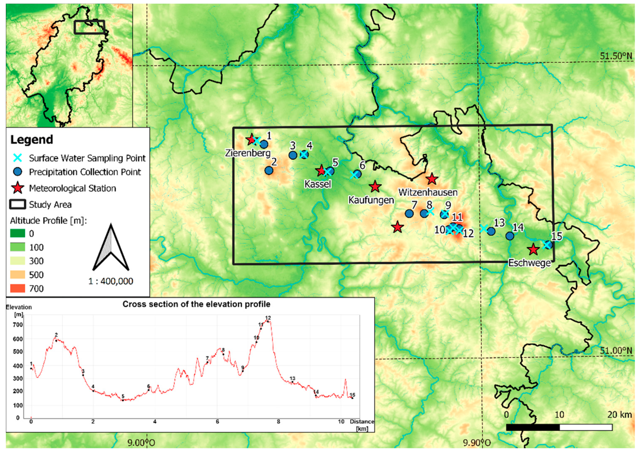
The Hessian uplands in Germany are bordered by the Rhenish Slate Mountains in the west (W) and the Thuringian Basin in the east (E). North Hesse is characterized by a densely forested low mountain range which includes the western part the Rothaar Mountains with a maximum elevation in the Hessian part (838 m), the Meissner (754 m) in the east, the Kellerwald (675 m) in the south-west (SW) as well as the Habichtswald (615 m) in the west and the Reinhardswald (472 m) in the north (N) [44]. Numerous depressions with river valleys cut through the low mountain ranges and form important catchment areas in North Hesse. Since the mountainous region of North Hesse is characterized by high reliefs, a study area was chosen that fairly presents the topographic features including elevations, depressions and slopes. The total study area covers approximately 120 km2 (Figure 1).
2.2. Climatic Conditions and Data Collection
The meteorological conditions over the entire period were investigated to check possible correlations with other parameters besides altitude. Meteorological data were provided by the Hessian State Office for Nature Conservation, Environment and Geology (HLNUG) from the weather stations, Kassel Mitte, Meissner/Witzenhausen, and Zierenberg for precipitation, temperature, air pressure, relative humidity (Rh), wind speed, and wind direction. More precipitation data were collected from Hessisch Lichtenau Fürstenhagen (HL), Eschwege, and Kaufungen stations of the German Weather Service (DWD). For the data evaluation, daily sums for precipitation and the daily mean values of other parameters were used. One regional meteorological station represents the climatic conditions for a few nearest individual precipitation collectors belonging to nearly the same meteorological conditions. All meteorological stations and the rainwater and surface water collection points are shown in Figure 1.
From a large-scale climatic point of view, Germany belongs to the extratropical west wind zone. The Atlantic Ocean is one of the main sources of precipitation in Germany [45]. Kassel is geographically assigned to the mid-latitudes and is characterized by a temperate climate but with latitudes of about 50°, it indicates a temperate humid, but also continental climate [46]. Therefore, the study area is mainly influenced by the SW wind zone and thus predominantly by Atlantic air masses. Partially, temperate dry winters can be assumed in the area and are thus also under the influence of polar, northern air masses [47]. During high-pressure weather conditions, the winds often come from the NE direction, as a secondary wind direction in addition to the SW main wind direction. Wind direction data collected from Kassel, Zierenberg, and Witzenhausen climate stations during the study period reported that the main directions were W and NW and also partially from SE directions for the Zierenberg area. For Kassel, the main wind direction was SW and partially from N and NE directions.
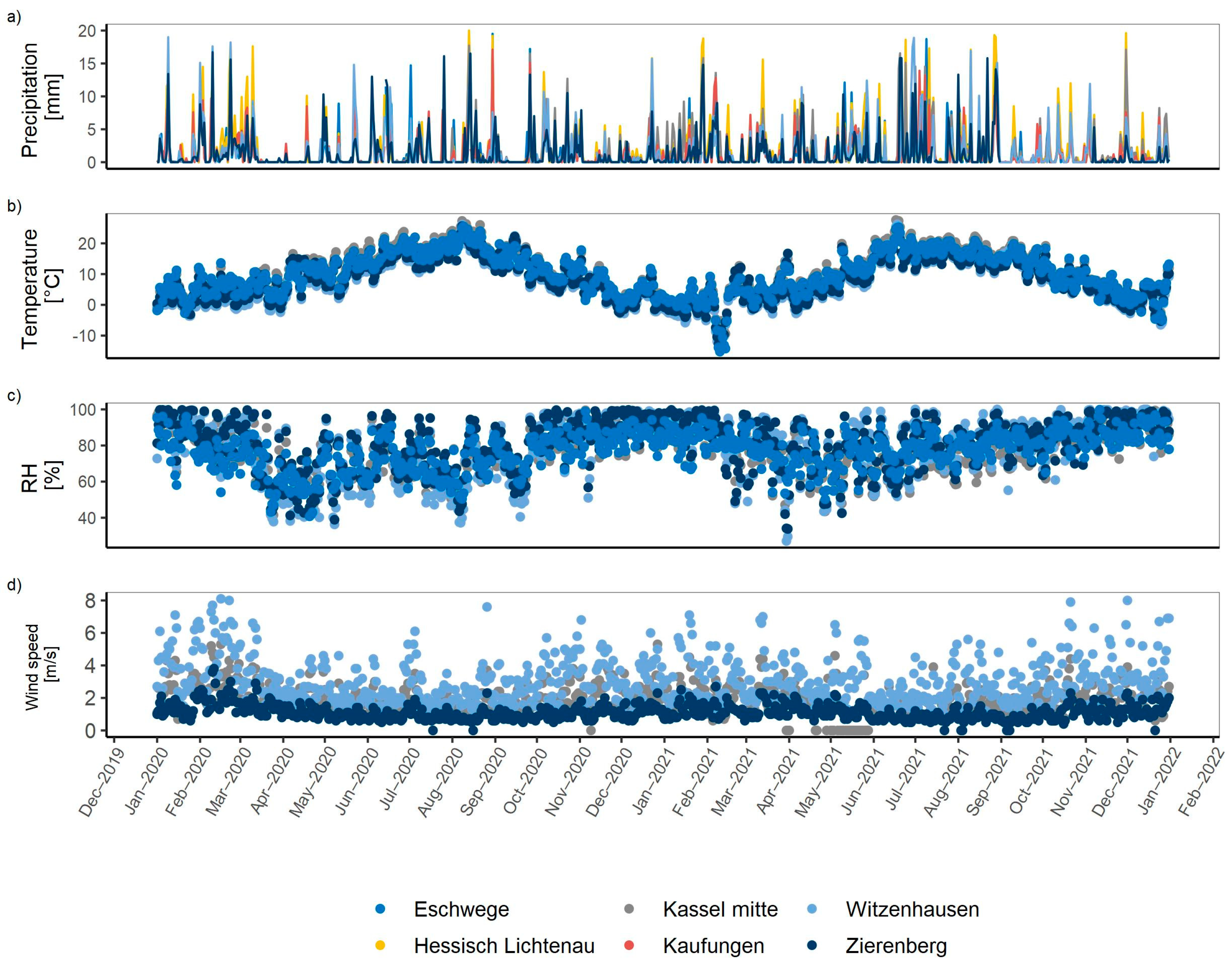
The selected study area covers an altitude range of 132–722 m. The precipitation amount varied greatly during the study period where the mean average value for 2020–2021 was 614 ± 146 mm (Appendix A, Figure A2). The lowest precipitation was reported for Zierenberg and Eschwege (510 ± 55 mm) while the highest was for HL (810 ± 138 mm). The temperature varied between 27.6 and −12.65 °C during the summer and winter and Rh was 75.8 ± 11.6%. Wind speed changes depending on the time of the year, however, the daily mean had varied 1.86 ± 0.94 ms−1 while the mean annual wind speed was reported as 3.5–4.0 ms−1 [48].
2.3. Measurement Profile
To create an altitude gradient for investigating the altitude effect, a measurement profile consisting of 15 low-cost rain gauges was designed along a transect of 60 km length, extending from Zierenberg in the NW of Kassel via HL to Eschwege in the SW of Kassel (Figure 1). To provide a structural overview, the measuring stations were divided into three areas which included Kassel: stations 1–6, HL/Meissner: stations 7–12, and Eschwege: stations 13–15 (Table 1). The designed measurement network represented an elevation gradient covering the entire height spectrum from 132 m (Kassel) to 722 m (Meissner) and approximately follows the transect of an appropriate altitude profile. In addition, each altitude level corresponding to 100 m was represented twice to guarantee the measurement reliability.
2.4. Construction and Installation of the Rainwater Precipitation Collectors
The design and installation of the precipitation collectors were based on the International Atomic Energy Agency brochure [49] for proper collection of rainwater for isotope analysis. Care was taken to minimize the influence of surrounding structures on the collectors including the height of surrounding vegetation (which should not exceed 0.5 m). The collectors were installed on undisturbed and naturally vegetated grasslands with slopes < 15%. The precipitation collectors had a maximum standing height of 0.3 m to minimize wind turbulence.
The heights at the sites were determined using a GPS and barometric measurements. A 500 mL high density polyethylene (HDPE) bottle (Lab Logistics Group GmbH, Meckenheim, Germany) was used as the precipitation collection container (Appendix A, Figure A1) and was placed approx. 0.1 m deep in the ground to minimize possible freezing processes and protect from evaporation. A 0.35 m long HT tube was served as a casing and fixed in the ground as a protection cover against the weather and other environmental influences. To effectively catch the precipitation, collection funnels with a diameter of 160–190 mm were placed on top of the high temperature (HT) pipes. A PVC tube routed the collected water directly from the funnel into the collection bottle. Possible air openings were closed and reinforced with sealing tape made of Flexible polyurethane foam with modified acrylates (SDF). A ping-pong ball was placed in each funnel, effectively closing the opening to minimize the evaporation processes. Finally, a fine-mesh polyester net was used to protect the structure from coarse debris.
Snow samples were collected during winter 2020 at stations placed above 400 m altitude. Surface water samples were also collected related to each elevation zone. The 11 selected surface water locations (decreased to 5 to reduce the sampling time from May 2021 after 65 samples) are shown in Figure 1 with the associated precipitation collectors. The rainwater was transferred weekly into 50 mL HDPE bottles using paper filters. All water samples were collected following the IAEA standard procedures [50]. The weekly cumulative integrated collection for one year gave us 465 rainwater and 156 surface water samples. Samples were stored in a dark, cold environment and later analyzed for δ18O and δ2H via wavelength-scanned cavity ring-down spectroscopy (WS-CRDS, L2130-i, Picarro, Santa Clara, CA, USA) at the laboratory for Urban Water Management and Water Quality, University of Kassel, Germany (analytic precisions for δ18O and δ2H are 0.025‰ and 0.1‰, respectively). Isotopic compositions are reported as ratios (R) of isotopes (2H/H, 18O/16O) in delta notation (δ [‰]) relative to the Vienna Standard Mean Ocean Water (VSMOW) [51] where δsample = (R/RVSMOW − 1). In addition, D-excess = δ2H − 8 δ18O was calculated. D-excess is a stable second-order isotope parameter that can be used to make statements on the source of precipitation and the evolution of moisture masses during transport [39] and it is also a proxy for evaporation processes [52]. The D-excess is in general 10‰ on a global average [40] and varies highly regionally, fluctuating between 0 and 20‰ [46]. Variations are often attributed to either moisture recycling or sub-cloud raindrop re-evaporation [53]. At local sites, seasonal variations in D-excess are mostly presented due to altitude, temperatures, amount of precipitation, or Rh variations. Isotopic compositions from each sampling station of each sampling date were plotted with the average precipitation and temperature between 2 sampling dates of the corresponding region to check the amount and temperature effects. All the gradients were calculated based on the slope of the linear regression line.
The average linear relationship of both water isotopes in global precipitation leads to the Global Meteoric Water Line (GMWL) and deviations depending on the local conditions result in Local Meteoric Water Lines (LMWL). In comparison to the GMWL in the dual isotope space, each local or regional line represents different idealized hydroclimatic scenarios due to the distributions of climatic zones [46] and helps to identify the environmental conditions during the sampling time. The GMWL was fitted by Rozanski et al. [41] as δ2H = 8.2 δ18O + 11.3 which was updated from its original form [4]. The LMWL of North Hesse was determined as δ2H = 7.52 δ18O + 7.4 by isotope data for the last 15 years from the IAEA/GNIP- WISER database system [43] from a station named “Kahler Asten” which is located nearly 50 km away from the study area.
2.5. Statistical Analysis
The normal distribution and the homogeneity of variances of the water isotopes were tested using Shapiro–Wilk test and Fligner–Killeen test (R 3.4.3), respectively. Because the data were not normally distributed, statistically significant differences were tested using the non-parametric rank-based Kruskal–Wallis test between different regions and seasons [54]. Null hypothesis is rejected, that there is no difference between the means, denoting that a significant difference does exist. Pearson correlation coefficients (r) were computed to find out the relationships between variables.
3. Results
3.1. Isotopic Distribution
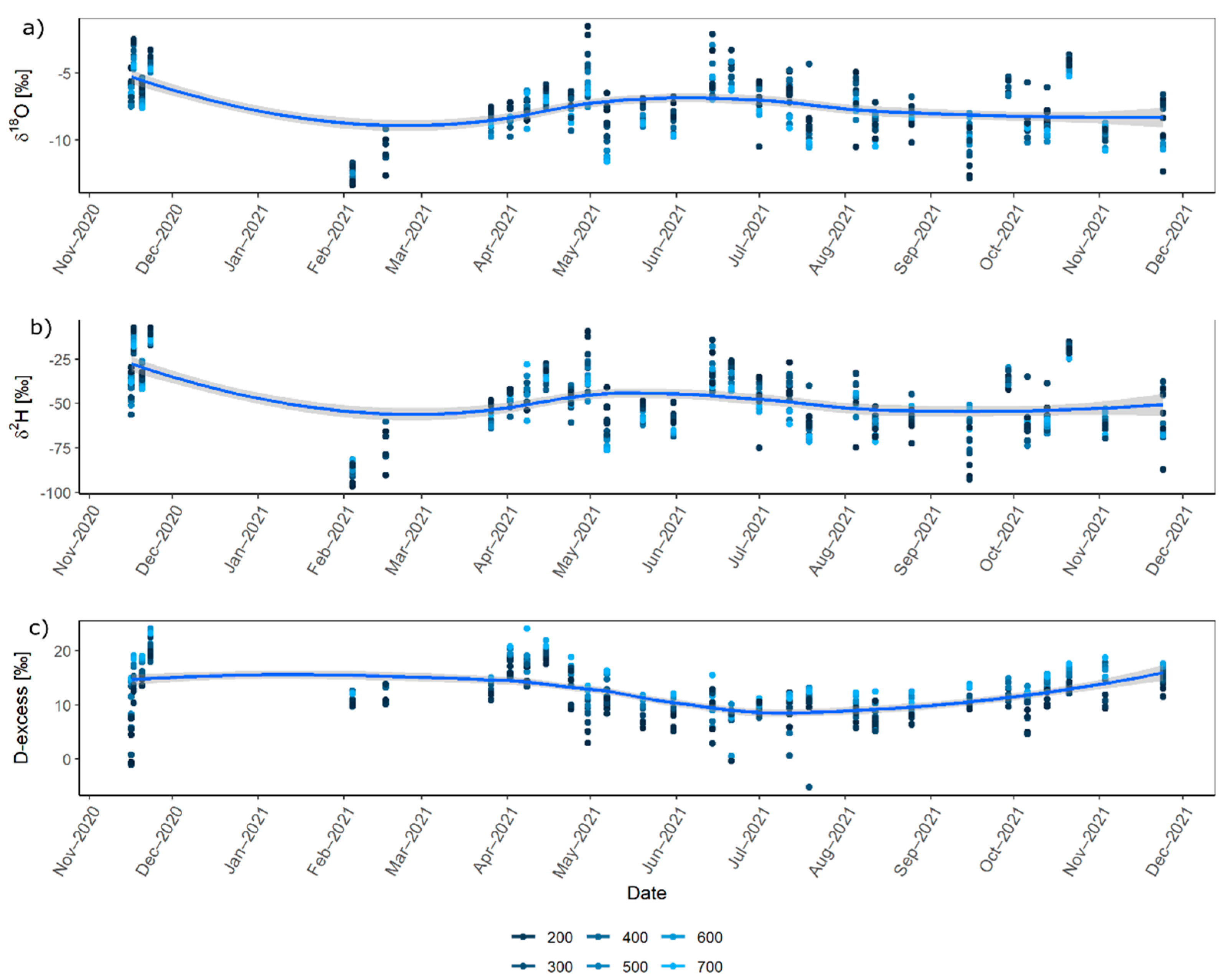
The fluctuations of isotopes of all the stations during the entire sampling period strongly reflected the seasonal changes and altitude differences. The non-linear curve-shaped fluctuation of the regression along the sampling period indicated a much more structured variation on a seasonal basis where the peaks (enriched values) were during summer, from June to August. Depleted values were mainly from February to May and September to January (Figure 2). The highest altitudes were plotted towards the lower values (depleted) for both isotopic compositions (Figure 2b) and the inverted profile was observed for D-excess (Figure 2c). The isotopic values from the 3 regions were not significantly different and follow the same fluctuations with slight variations.
The average isotopic composition of the precipitation varied between −1.54 and −13.34‰ for δ18O, −7.23 and −96.55‰ for δ2H in the entire altitude profile during the study time except for snow samples (Table 2). However, significant variations between the measurements from the individual stations were noted. The most enriched values were observed mostly from the stations of lower elevations such as Niederduenzebach (153 m), Eschwege (185 m), Kassel (132 m), Harleshausen-FH (201 m) and Harleshausen-P (323 m) while depleted values were observed in the highest elevations such as Meissner-Kurve (669 m), Meissner-Top (722 m) and Habichtswald (555 m). Furthermore, most depleted values were encountered as snow in February 2021 from Helsa (432 m, δ18O = −19.02‰, δ2H = −137.89‰).
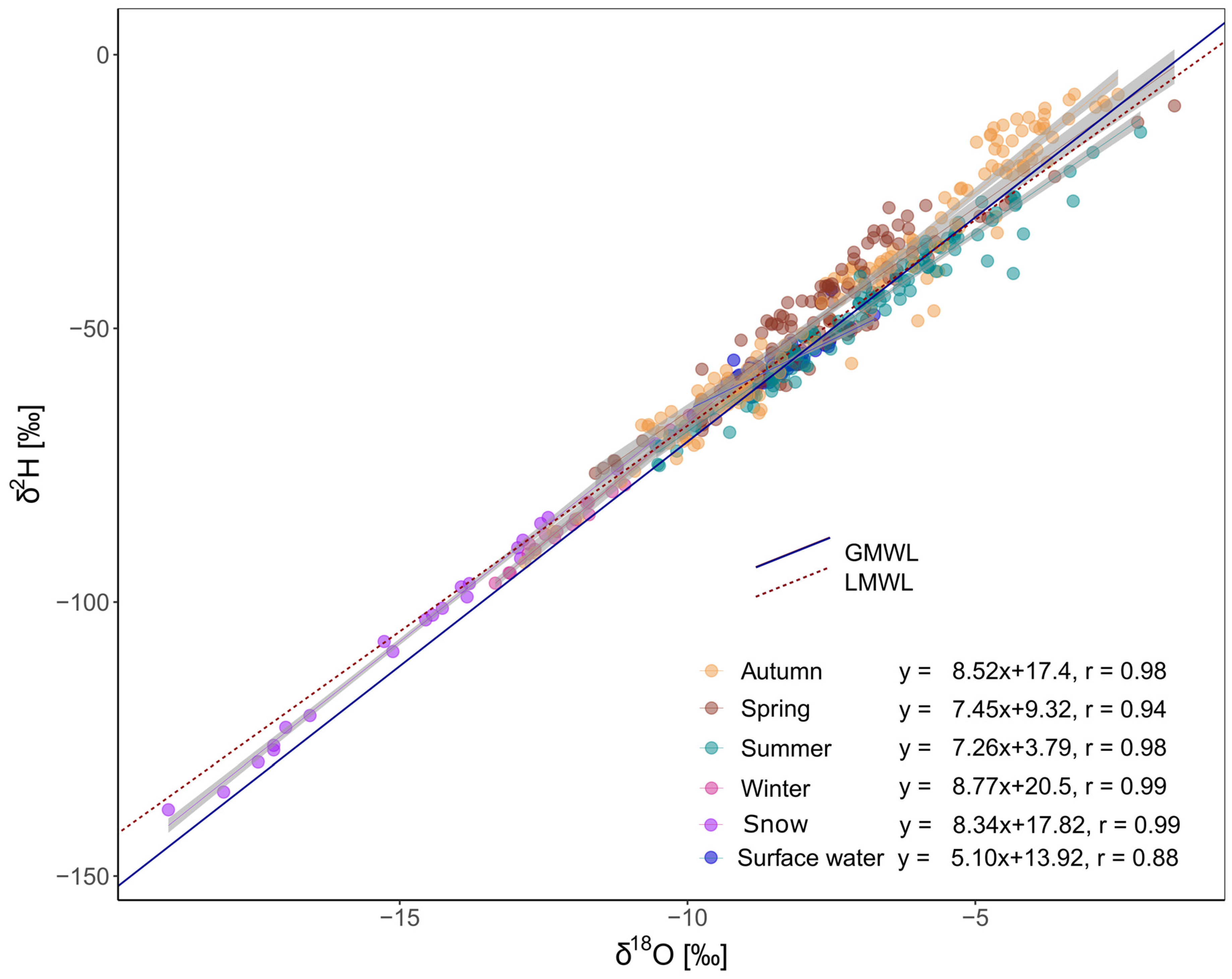
The values of δ18O and δ2H followed the GMWL and LMWL with slight deviations (Figure 3). The snow samples were separated and plotted on the lower left side above the GMWL representing colder climatic conditions (δ2H = 8.3 δ18O + 17.8, r = 0.99) while the summer data were mostly plotted at the top right section of the line. However, there were some deviations from the mean waterline. All rainwater samples followed an intermediate slope, higher than the slope of the LMWL for the area and closer to the GMWL, which could be written as δ2H = 8.0 δ18O + 12.2 (r = 0.97). The slopes based on seasons are autumn = 8.5 (r = 0.98), spring = 7.4 (r = 0.94), summer = 7.3 (r = 0.98), and winter = 8.7 (r = 0.99). The slope of the summer was the lowest showing a higher deviation from the GMWL. The lower elevations (<500 m) were plotted in the upper part of the waterline with a slope of around 8, while the higher elevations (>500 m) were plotted in the lower part having a slightly higher slope of around 8.6. The slope of surface water of 5.1 (r = 0.88) was lower than the rainwater, showing the influence of evaporation. The regional differences were also visible in the dual isotope plot, where the highest slope was observed for HL/Meissner (8.18, r = 0.97), while the lowest was observed for Kassel (8.07, r = 0.97) and Eschwege (8.07, r = 0.98), without any significant difference. The values plotting far above the LMWL were characterized by very high D-excess (>20‰) while extremely low D-excess values (<2‰) were located below the waterline.
3.2. Altitude Effect
The altitude gradient varied depending on the climatic conditions and the sampling time. The isotopic compositions disclosed a negative correlation with increasing altitude. A strong correlation with altitude having the highest negative slope was observed during March 2021 (r = −0.7, p < 0.01) for both isotopes. However, high standard deviations of up to ± 42‰ resulted from snow events and thus no trend could be predicted in February 2021 (δ18O, r = −0.03, p = 0.91 and δ2H, r = −0.06, p = 0.79). At an elevation between 435–722 m, the most depleted isotope values were observed as snow samples (Table 2).
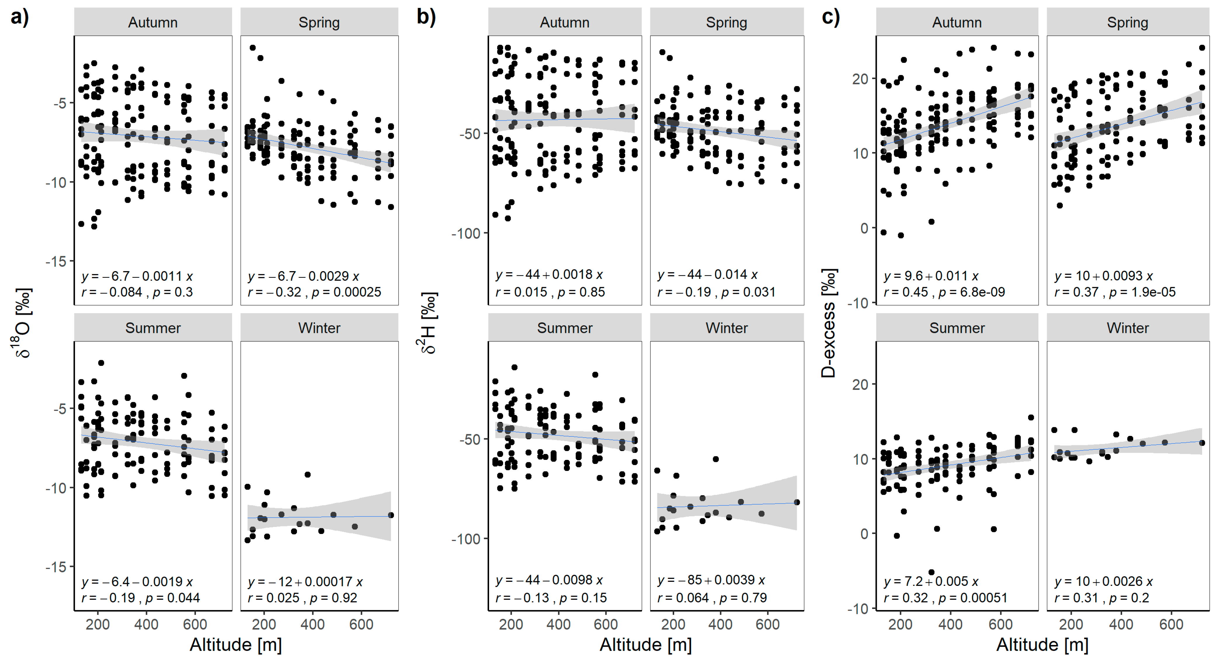
The overall gradients between isotope values and altitude for the entire sampling period were −0.14‰/100 m (r = −0.11, p = 0.01) for δ18O and −0.28‰/100 m (r = −0.03, p = 0.57) for δ2H. Slightly positive correlations were observed in August and September 2021. Furthermore, the altitude gradient illustrated seasonal variations, where it was significant in spring (−0.29‰/100 m for δ18O, r = −0.32, p < 0.001 and −1.4‰/100 m for δ2H, r = −0.19, p = 0.03) (Figure 4a,b). However, the positive correlation with D-excess was stronger than individual isotopes (Figure 4c) and it was 0.83‰/100 m (r = 0.33, p < 0.001) for the study period and presented a higher gradient of 1.2‰/100 m in May and November 2022. Overall, the mean D-excess values were 10.68 ± 3.90‰, 13.7 ± 4.40‰, and 11.58 ± 4.47‰ for Eschwege, HL/Meissner, and Kassel regions, respectively. The highest D-excess values (>23‰) were measured in higher elevations > 600 m while the lowest values (<1‰) were observed at the lower elevation (<300 m). The seasonal correlations between altitude and D-excess were more significant than with individual isotopes (0.5–1.1‰/100 m, r = 0.3 − 0.4, p < 0.001) except for winter due to the snow events.
3.3. Amount Effect
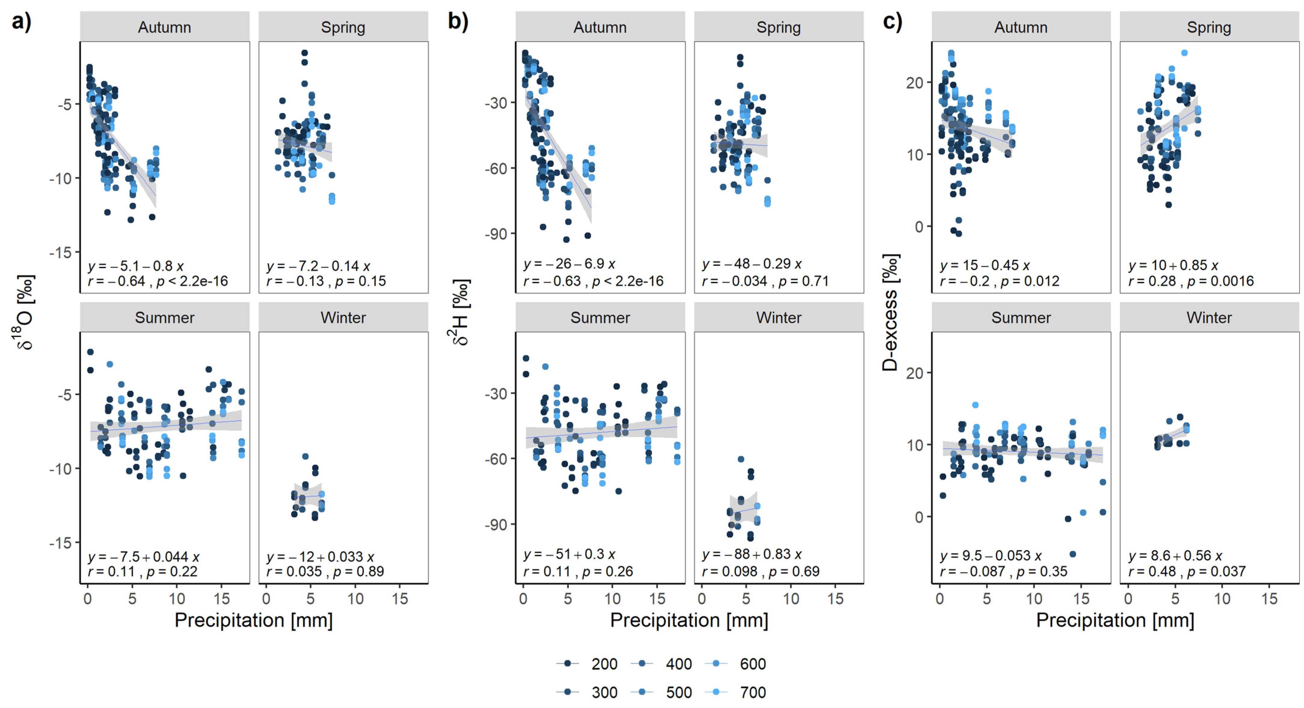
The amount effect is the tendency for higher amounts of precipitation to be more isotopically depleted. Depletion of isotopes with increasing precipitation amount was observed for the entire study period even though it was a low, yet significant correlation (mostly p < 0.001) with −0.059‰/mm for δ18O (r = −0.10), −0.83‰/mm (r = −0.17) for δ2H and −0.36‰/mm (r = −0.32) for D-excess. The most enriched values were observed with a precipitation amount of <1 mm/day, while the most depleted values were in high precipitation events (>10 mm/day). However, this also depended on the other climatic variables and the type of the event such as snowfalls.
Figure 5a,b show a significantly negative correlation between isotope values and the precipitation amount (p < 0.001) in autumn (−0.8‰/mm for δ18O, r = −0.64 and −6.9‰/mm for δ2H, r = −0.63), but no significant correlations (p > 0.05) were observed in summer (δ18O 0.04‰/mm, r = 0.11 and δ2H 0.3‰/mm, r = 0.12), winter (δ18O 0.03/mm, r = 0.03 and δ2H 0.83‰/mm, r = 0.10) and spring (δ18O −0.14‰/mm, r = −0.13 and δ2H −0.29‰/mm, r = −0.03). However, in winter, the sample size was small and also there were some deviations due to the snow events. The D-excess (Figure 5c) indicated a positive correlation to precipitation amount (p < 0.05) during spring (0.85‰/mm, r = 0.28), winter (0.56‰/mm, r = 0.48), and autumn (−0.45‰/mm, r = −0.20) but no correlation during summer (−0.053‰/mm, r = −0.09, p = 0.35). Sometimes the higher precipitation amounts during the study period had no large-scale influences on the isotope distribution. This can be attributed in part to the fact that detailed precipitation amounts were not available for each collection point due to limited meteorological stations, and consequently, one weather station represented multiple collection sites.
3.4. Temperature Effect
During the total study period, a positive correlation with temperature was detected, i.e., enrichment of the heavy isotopes with increasing temperature for δ18O with 0.07‰/°C (r = 0.19, p < 0.001) but not for δ2H (0.15‰/°C, r = 0.05, p = 0.32). However, the correlations were significant when separated by seasons (P < 0.001), except for spring (Figure 6). The temperature range was high during the spring and autumn (~−2–20 °C) compared to summer (~12–25 °C) and winter (~−12–11 °C). Rising temperatures regularly caused an average enrichment of isotopic composition in precipitation especially in summer, while depletion of isotopes could also be observed with increasing temperature conditions, especially in autumn (Figure 6a,b). The negative gradient was significant (p < 0.001) in autumn (δ18O −0.2‰/°C, r = −0.30 and δ2H −2.3‰/°C, r = −0.40) and winter (δ18O −0.23‰/°C, r = −0.68 and δ2H −2‰/°C, r = −0.69). Although there was a significant correlation for δ2H in spring (−0.75‰/°C, r = −0.21, p = 0.02), no correlation was observed for δ18O (−0.003‰/°C, r = −0.01, p = 0.94), while a positive significant gradient was detected in summer (δ18O 0.38‰/°C, r = 0.46 and δ2H 2.7‰/°C, r = 0.43, p < 0.001). In the temperature range <0 °C, the values were significantly more depleted than the average (p = 0.001, r = −0.7), and this was exclusively the case for the snow samples. However, snow samples were not included in the calculation and were considered as outliers. The negative correlation of D-excess with temperature was stronger (0.41‰/°C, r = −0.56, p < 0.001) over the whole period (Figure 6c). The gradients of D-excess were more prominent for autumn and spring (−0.7‰/°C, r = −0.60, p < 0.001) than the individual isotopes. The highest D-excess (>20‰) was measured at a temperature below 5°C, belonging to altitudes >500 m, while the lowest values (<5‰) were found at a temperature > 15 °C at altitudes < 300 m.
3.5. Surface Water
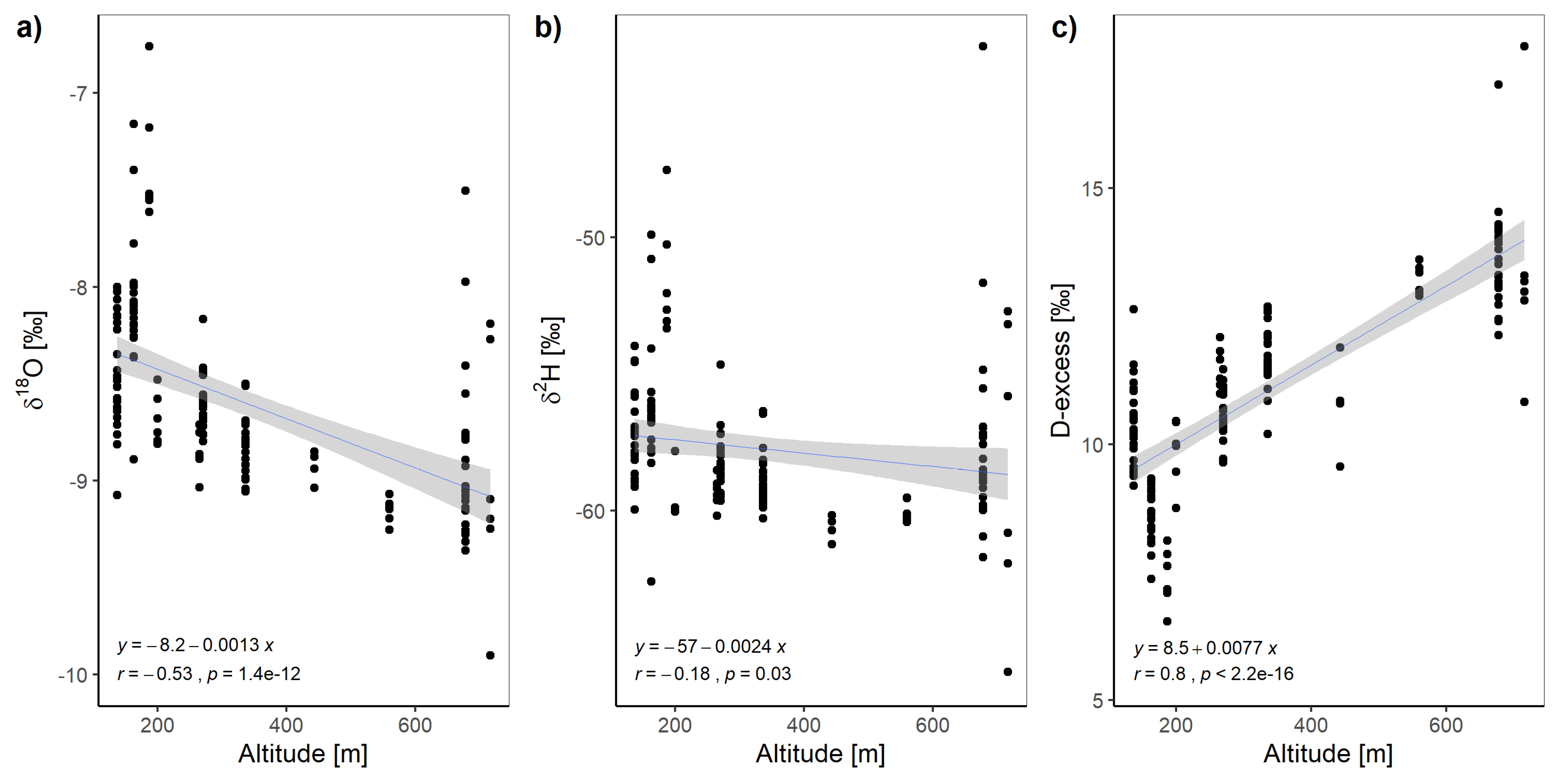
Isotopic variations between events were relatively small in the surface water locations (Figure 7). The average values were for δ18O −8.60 ± 0.47‰ and δ2H −57.73 ± 2.77‰ during the sampling period. A clear negative linear trend indicates a slight depletion of heavy isotopic composition with increasing elevation (for δ18O, −0.13‰/100 m, r = 0.53, p < 0.001 and δ2H, −0.24‰/100 m, r = 0.17, p = 0.03). A strong positive trend with increasing altitude for the D-excess was detected (0.77‰/100 m, r = 0.80, p < 0.001). The isotopic composition of the surface water was more depleted than the precipitation of the equivalent elevations but in winter and autumn 2021 it was more enriched. Although strong differences in the stable isotopic composition can be seen between the individual precipitation events, the variation in surface water was minimal throughout the study period. However, the D-excess values in the surface water were higher than in precipitation during the summer representing the effect of evaporation.
4. Discussion
4.1. Isotopic Distribution
The isotopic enrichment in the summer months (Figure 2) could be a consequence of higher surface temperatures [26,55] and more enriched local water vapor [56]. During winter, the precipitation can be influenced by the continental effect due to the moisture-bearing fronts, whereby frontal precipitation becomes progressively depleted in heavy isotopes and decreases in amount as it passes across the latitudes causing depleted troughs (Figure 2). Condensation processes are also responsible for the isotopic depletion during winter which has also been observed in the Adriatic-Pannonian region of south-eastern Europe [22].
Slope deviations may occur compared to GMWL in the dual isotope space due to kinetic fractionation [25] and the evaporation effect [4]. In Figure 3, the slope (8.0) and the intercept (12.2) of the water line for precipitation during this study was higher than the reference LMWL (slope = 7.5, intercept = 7.4), which could be a result of the climatic and physical condition changes in the study period. For example, primary and secondary evaporation could have lowered the slope and intercept, where secondary evaporation was particularly influential during low magnitude precipitation events [57]. Therefore, a lower evaporation effect could have occurred in the study area during the measurement period compared to the conditions under which the LMWL was derived. Apart from that, the LMWL was developed using the isotopic values from Kahler Asten which is nearly 50 km away from our study site. Stumpp et al. [1] have also obtained a similar slope of 7.6 for Kahler Asten. The lower part of the water line mainly contained measurements from higher elevations > 400 m, and snow samples, confirming cold winter conditions [46]. The upper part contained lower elevations < 400 m also agreeing with the findings by Xi [58]. Stations that had low D-excess values (<10‰) plotted below the LMWL with a lower slope, especially in the summertime, suggesting secondary evaporation processes i.e., evaporation of falling raindrops [59]. Deviations above the LMWL with high D-excess (>20‰) in spring and also at the end of autumn indicate high humidity conditions [52,60]. The higher slopes compared to the GMWL also suggest continental recycling processes during autumn and winter. Mixed-phase cloud formation creates higher slopes and the influence of these effects varies by season [46], which was also more apparent during winter in our study. The slope of our water line is higher than the slopes derived as 7.7 for Germany [1], 6.8 for Valentia (Ireland) and 7.2 for Groningen (Netherlands) by the long-term records (GNIP, 2002) [3]. Regression analysis by Hager and Foelsche [28] found that isotopic values were controlled by temperature on a temporal basis, while altitude is the dominant factor on a spatial basis which gives a good explanation to our observations based on the water line.
Rh variations during warmer periods together with temperature (Appendix A, Figure A2) create a stronger evaporative effect and altered the slopes of the regression lines. The slope of the dual isotope plot for Rh between 25–75% was found to be ~5 for open water bodies [61], while we observed 5.1 for surface water (Figure 3) under the Rh between 65–95%. The amount evaporated from surface water bodies depends on the meteorological conditions and the time of exposure to the atmosphere [62]. Thus, in our study, surface water during the summer was subject to more evaporation supported by more enriched values than during the colder months.
4.2. Altitude Effect
The focus was to understand local fluctuations of isotopic composition (δ18O and δ2H) in precipitation mainly with altitude on a regional scale (Figure 4a,b). A progressive decrease in both isotopic compositions in precipitation with increasing elevation resulting from the cooling of air masses was often observed, which is known as the altitude effect [26]. Elevation patterns have frequently not been observed within mountains, in snow, as well as on the lee side of mountains [63] because the altitude effect is mostly superimposed by other effects such as amount, temperature, and orographic effects [64]. The altitude gradient generally ranges from −0.15 to −5‰/100 m for δ18O [4], while we observed an altitude gradient of −0.14‰/100 m for δ18O and −0.28‰/100 m for δ2H, in the mountainous region of North Hesse, which is lower than what has been observed for the whole of Germany (−0.47‰/100 m) [1], however comparable to Europe: to Italy (−0.2‰/100 m [65], to the UK (−0.2 to −0.3‰/100 m) [26] and to the global gradient (−0.2‰/100 m) [66]. The gradient for δ18O placed within the range of −0.1‰ to −0.6‰/100 m declared by the IAEA (2001) and Kern et al. [22] of −0.12‰/100 m in Eastern Europe. In parallel, altitude effects have been observed for δ18O of about −0.3‰/100 m in winter, and −0.2‰/100 m in summer at the British Isles [26] and −0.15 to −0.22‰/100 m in summer and −0.6‰/100 m in winter in the Swiss Alps [67].
Local effects are important when the gradients are calculated for a limited range of latitudes on a small scale. Theoretically, the D-excess increases with increasing altitude on the windward side of mountain slopes and marks a decrease in the leeward side making comparatively dry conditions [39] due to the orographic effect and rainout processes [4,68,69]. This phenomenon was observed in the mountainous region of North Hesse (Figure 4c). For example, higher precipitation was regularly measured for the Kassel region on the windward side of the Meissner than for the Eschwege region, which lies on the leeward side. The stations in the Eschwege region sometimes had the most depleted heavy isotope values (−17‰ for δ18O and −122‰ for δ2H), although it is a low altitude (<200 m) and in a comparatively higher average temperature range. When air masses meet orographic elevations, they tend to rainout more on the windward side and this effect led to a strong depletion on the leeward side of the Meissner (Figure 1). Lower D-excess values, which were mostly observed during summer (Figure 4c), may have occurred due to secondary evaporation and mixing processes of moisture sources [24,52]. At higher altitudes, the secondary evaporation phenomenon is less dominant because of lower temperatures and the shorter distance to the cloud base [59]. However, on an annual scale, such dependencies become less prominent and result in low correlations of D-excess with elevation and other parameters [12], as observed in winter (Figure 4c). The correlation of isotopic composition and D-excess of the surface water with the elevation indicated an expression of the altitude effect (Figure 7). Surface water was more enriched than the isotopic composition in precipitation because it may have been subjected to various fractionation processes, recharge, and mixing processes with groundwater and other catchment tributaries while flowing, similar to other studies [23,70,71,72]. Evaporation was confirmed in this study via the slope of the water line of surface water samples.
4.3. Amount Effect
The amount effect can be found progressively at latitudes < 30° and at mid-latitudes [28], which is also valid for our study site. Enriched isotope values were mostly related to low precipitation amounts (Figure 5). Precipitation during winter tends to be more isotopically depleted due to depleted moisture sources than in the summer [4]. Overall, quantitative gradients of −0.059‰/mm for δ18O, and −0.83/‰/mm for δ2H were observed, although Gonfiantini et al. [73] measured a smaller quantitative gradient of −0.014‰/mm in Bolivia. Relatively high precipitation and lower temperatures led to a depletion of the isotope values at individual sites e.g., the station “Harleshausen-FH” showed a depleted δ2H value of −17.23‰ on 23 November 2020, despite its low elevation of 201 m. The amount effect was more pronounced during autumn and spring and was weaker during winter and summer. Isotopes are partially controlled by other factors such as amount and temperature together with the elevation in our study site, similarly in some cities in Europe such as Stuttgart (Germany), Bern and Grimsel (Switzerland), Groningen (Netherlands) [74]. A negative correlation of isotopes with precipitation amounts in autumn and spring (Figure 5a,b) was also observed in Cape Town, Valentia, Antalya, and Puerto Montt [3], suggesting the influence of larger-scale convective processes on precipitation. This is probably one reason for the susceptible trends, with the amount effect additionally being a dominant factor that attenuates the altitude and the temperature effects. However, in some studies, no correlations were observed between isotopes and precipitation amount or elevation [23]. During spring, the amount effect was prominent in HL/Meissner while for Eschwege, it was suppressed by the orographic effect due to the location at the leeward side. In the summer months, low D-excess values (<10‰) signified high evaporation (Figure 5c). Similarly, more enriched isotopic and lower D-excess values during warmer periods have been observed at other European sites [75].
4.4. Temperature Effect
Temperature is the major governing parameter for isotope fractionation, and it significantly influences the altitude effect. Fractionation is temperature dependent and higher in cold environments than in warm, and consequently results in greater depletion of heavy isotopes at low temperatures [4]. This effect was observed during this study (Figure 6), especially in snow events, which produced strongly depleted values at ground temperatures < 2 °C.
A positive correlation of temperature with isotopes during summer was observed and the gradient of 0.38‰/°C for δ18O is slightly lower than the value in the literature of 0.58‰/°C for Europe [27] and similar to the normalized values for Braunschweig (0.35‰/°C) and Kahler Asten (0.32‰/°C) in Germany [1]. It was slightly higher than the values from GNIP stations at Valentia and Groningen of 0.32‰/°C and an 11-year time period of 0.22‰/°C in the British Isles [26]. The negative gradient of −0.35‰/°C measured in Austria by Hager and Foelsche [28] is also comparable to the gradients during autumn and winter in our study (−0.2‰/°C). A similar seasonal observation was reported for Heidelberg, Germany [76], and explained by different proportions of admixing of air masses transported to the region. Depending on the location, the relationship may vary, and it has been reported between 0.14–0.42‰/°C for δ18O in the East and South compared to the West and North of Germany [1], which is comparable to our results except during spring (Figure 6a).
The fluctuations in D-excess during the seasons (Figure 6c) are controlled by local factors, for example, the sub-cloud evaporation could decrease and moisture recycling could increase the D-excess [52,77]. During summer, the precipitation may have been influenced by the recycled land moisture rather than by oceanic moisture sources because higher temperatures and lesser precipitation suggest secondary evaporation effects [25] and the rise of sub-cloud evaporation [52,74,78]. The positive correlation with isotopes and negative with D-excess during warmer months in this study suggests a higher contribution of recycled moisture which has also been observed in Stuttgart, Germany [74]. In contrast, the negative correlation of temperature with isotopes and with D-excess reveal a lower temperature effect during the colder months, especially during autumn and winter. A diminished temperature effect is also possible due to the depleted oceanic moisture sources compared to the recycled moisture during colder months [52,79]. A negative correlation was also observed in Addis Ababa, Antalya, Puerto Montt, and Valentia [3] which was due to the decreased supply of recycled moisture and increase in temperature.
The lack of clear and strong linear relationships could also suggest a non-linear relationship between the isotopic composition with altitude, temperature, and precipitation amount. This could be a result of the control of multiple external and local factors including large-scale convective processes which affect the local conditions [10,30,52,61,67,70,72,80]. The direct and strong impact of oceanic moisture and air masses from different sources may have weakened the trend and neglected the influence of the landmass at sometimes [74,81,82].
4.5. Limitations of the Study and Potential Improvements
There were some limitations and difficulties maintaining such manual rain gauges for a long period such as low durability of the materials, damages to the rain gauges, vandalism, physical effort, high transportation costs and time for sampling together with subsequent laboratory analysis. Moreover, problems in manual sample collection followed by transport, storage, labor power and time are also considerable issues. These factors limited the frequency and duration of sampling.
Improvements could be made in future studies by using more informative precipitation collection stations such as quantitative rainfall sampling at each station, sequential samplers for fixed volumes or time steps [23], or high-resolution direct precipitation isotope measurements using field laser spectroscopes [42,70,83]. Moreover, adding more replicates at each elevation zone representing topographic features or reducing the distance between collectors may support clearer statistical results. More frequent data collection, for example, a measurement after each event or several measurements within an event would provide more accurate predictions.
5. Conclusions
The observation of an one-year period provides the first insights into the isotope distribution over a larger area in North Hesse. An expression of the altitude gradients of −0.14‰/100 m for δ18O, −0.28‰/100 m for δ2H, and 0.83‰/100 m for D-excess supported that isotopes become increasingly enriched with increasing altitude even at a small scale. However, an expression of direct altitude effect on the stable isotopic composition cannot be defined due to the influence of other factors such as temperature, precipitation amount, mixing processes, orographic rainout process, moisture recycling and sub-cloud evaporation. The mixing of moisture sources due to evaporation and secondary evaporation has increased during summer while condensation processes with depleted oceanic moisture fronts were more dominant during winter. The amount effect was more predominant in autumn and spring, together with continental recycling processes in high elevated areas and large-scale convective processes. The amount effect was suppressed by orographic and temperature effects for the Eschwege region, located on the leeward side of Meissner. The slope of the local meteoric waterline for the study period (8.0) was higher than the existing LMWL, presenting a temporal fluctuation of enrichment during warmer periods and depletion in colder periods. Isotopic composition of surface water indicated an altitude effect yet did not show high fluctuations during the study period although it had been subjected to evaporation.
It was demonstrated that the stable isotopes of water and D-excess are strong tools to unravel the processes for the formation of precipitation in complex terrain. Multiple stations and frequent data collection provide detailed information about the dependencies and influences on individual variations at the regional scale. Thus, using LMWLs from reference stations nearby might still lead to significant errors in estimating isotopic signals of rainfall regionally due to local influencing factors. Therefore, a proper measurement profile may serve as a better basis to investigate the long-term behavior of stable isotopes of water in mountainous regions, providing insights into hydrological and climatic processes on a regional scale. Using stable isotope data from a single precipitation measurement station as often used, e.g., for deriving transit time distributions in hydrology, might not be representative in a complex relief. More frequent data would make it possible to capture different factors influencing seasonal and spatial stable water isotope variations in a complex process interplay.
Author Contributions
Conceptualization, A.M. and M.G.; Data curation, A.M. and M.J.; Formal Analysis, A.M. and M.J.; Investigation, A.M. and M.J.; Methodology, A.M., M.J. and M.G.; Resources, M.G. and A.M.; Software, A.M. and M.J.; Supervision, M.G. and A.M.; Visualization, A.M. and M.J.; Writing, A.M. and M.J.; Review and Editing, M.G. and A.M.; Funding Acquisition, M.G. All authors have read and agreed to the published version of the manuscript.
Funding
This research received no external funding.
Data Availability Statement
The data used in this paper are available from A.M. ([email protected]) upon request.
Acknowledgments
We acknowledge, with gratitude, the sampling support from Tarik Schulz and Gabriel Schmid; laboratory support from the Department of Urban Water Management at the University of Kassel; and discussions with Jayan Wijesingha.
Conflicts of Interest
The authors declare no conflict of interest.
Appendix A
Figure A1.
A schematic diagram of a precipitation collector.

Figure A2.
Fluctuations of climatic variables, precipitation (a), temperature (b), relative humidity—RH (c), wind speed (d) variation during the experimental years (2020–2021).
Figure A2.
Fluctuations of climatic variables, precipitation (a), temperature (b), relative humidity—RH (c), wind speed (d) variation during the experimental years (2020–2021).

References
- Stumpp, C.; Klaus, J.; Stichler, W. Analysis of Long-Term Stable Isotopic Composition in German Precipitation. J. Hydrol. 2014, 517, 351–361. [Google Scholar] [CrossRef]
- Vreča, P.; Krajcar Bronić, I.; Leis, A. Isotopic composition of precipitation in Portorož (Slovenia). Ruđer Bošković Inst. 2011, 54, 129–136. [Google Scholar] [CrossRef]
- Vystavna, Y.; Matiatos, I.; Wassenaar, L.I. Temperature and Precipitation Effects on the Isotopic Composition of Global Precipitation Reveal Long-Term Climate Dynamics. Sci. Rep. 2021, 11, 18503. [Google Scholar] [CrossRef] [PubMed]
- Clark, I.D.; Fritz, P. Environmental Isotopes in Hydrogeology; CRC Press: Boca Raton, FL, USA, 1997; ISBN 978-1-56670-249-2. [Google Scholar]
- Qian, H.; Wu, J.; Zhou, Y.; Li, P. Stable Oxygen and Hydrogen Isotopes as Indicators of Lake Water Recharge and Evaporation in the Lakes of the Yinchuan Plain. Hydrol. Process. 2014, 28, 3554–3562. [Google Scholar] [CrossRef]
- Ma, H.; Yang, Q.; Yin, L.; Wang, X.; Zhang, J.; Li, C.; Dong, J. Paleoclimate Interpretation in Northern Ordos Basin: Evidence from Isotope Records of Groundwater. Quat. Int. 2018, 467, 204–209. [Google Scholar] [CrossRef]
- Adomako, D.; Maloszewski, P.; Stumpp, C.; Osae, S.; Akiti, T.T. Estimating Groundwater Recharge from Water Isotope (Δ2H, Δ18O) Depth Profiles in the Densu River Basin, Ghana. Hydrol. Sci. J. 2010, 55, 1405–1416. [Google Scholar] [CrossRef] [Green Version]
- Bedaso, Z.; Wu, S.-Y. Linking Precipitation and Groundwater Isotopes in Ethiopia—Implications from Local Meteoric Water Lines and Isoscapes. J. Hydrol. 2021, 596, 126074. [Google Scholar] [CrossRef]
- Mahindawansha, A.; Orlowski, N.; Kraft, P.; Rothfuss, Y.; Racela, H.; Breuer, L. Quantification of Plant Water Uptake by Water Stable Isotopes in Rice Paddy Systems. Plant Soil 2018, 429, 281–302. [Google Scholar] [CrossRef]
- Mahindawansha, A.; Külls, C.; Kraft, P.; Breuer, L. Investigating Unproductive Water Losses from Irrigated Agricultural Crops in the Humid Tropics through Analyses of Stable Isotopes of Water. Hydrol. Earth Syst. Sci. 2020, 24, 3627–3642. [Google Scholar] [CrossRef]
- Kulkarni, T.; Gassmann, M.; Kulkarni, C.M.; Khed, V.; Buerkert, A. Deep Drilling for Groundwater in Bengaluru, India: A Case Study on the City’s Over-Exploited Hard-Rock Aquifer System. Sustainability 2021, 13, 12149. [Google Scholar] [CrossRef]
- Liu, Z.; Bowen, G.J.; Welker, J.M. Atmospheric Circulation Is Reflected in Precipitation Isotope Gradients over the Conterminous United States. J. Geophys. Res. Atmos. 2010, 115, D22120. [Google Scholar] [CrossRef] [Green Version]
- Vachon, R.W.; Welker, J.M.; White, J.W.C.; Vaughn, B.H. Monthly Precipitation Isoscapes (Δ18O) of the United States: Connections with Surface Temperatures, Moisture Source Conditions, and Air Mass Trajectories. J. Geophys. Res. Atmos. 2010, 115, D21126. [Google Scholar] [CrossRef]
- Welker, J.M. Isotopic (Δ18O) Characteristics of Weekly Precipitation Collected across the USA: An Initial Analysis with Application to Water Source Studies. Hydrol. Process. 2000, 14, 1449–1464. [Google Scholar] [CrossRef]
- Lykoudis, S.P.; Argiriou, A.A. Temporal Trends in the Stable Isotope Composition of Precipitation: A Comparison between the Eastern Mediterranean and Central Europe. Theor. Appl. Climatol. 2011, 105, 199–207. [Google Scholar] [CrossRef]
- Sturm, K.; Hoffmann, G.; Langmann, B.; Stichler, W. Simulation of Δ18O in Precipitation by the Regional Circulation Model REMOiso. Hydrol. Process. Int. J. 2005, 19, 3425–3444. [Google Scholar] [CrossRef]
- Taylor, K.E.; Stouffer, R.J.; Meehl, G.A. An Overview of CMIP5 and the Experiment Design. Bull. Am. Meteorol. Soc. 2012, 93, 485–498. [Google Scholar] [CrossRef] [Green Version]
- Bowen, G.J. Isoscapes: Spatial Pattern in Isotopic Biogeochemistry. Annu. Rev. Earth Planet. Sci. 2010, 38, 161–187. [Google Scholar] [CrossRef] [Green Version]
- Bowen, G.J.; Wassenaar, L.I.; Hobson, K.A. Global Application of Stable Hydrogen and Oxygen Isotopes to Wildlife Forensics. Oecologia 2005, 143, 337–348. [Google Scholar] [CrossRef]
- Sjostrom, D.J.; Welker, J.M. The Influence of Air Mass Source on the Seasonal Isotopic Composition of Precipitation, Eastern USA. J. Geochem. Explor. 2009, 102, 103–112. [Google Scholar] [CrossRef]
- Terzer-Wassmuth, S.; Wassenaar, L.; Welker, J.; Araguás, L. Improved High-Resolution Global and Regionalized Isoscapes of δ18O, δ2H, and d-Excess in Precipitation. Hydrol. Process. 2020, 35, e14254. [Google Scholar] [CrossRef]
- Kern, Z.; Hatvani, I.G.; Czuppon, G.; Fórizs, I.; Erdélyi, D.; Kanduč, T.; Palcsu, L.; Vreča, P. Isotopic ‘Altitude’ and ‘Continental’ Effects in Modern Precipitation across the Adriatic–Pannonian Region. Water 2020, 12, 1797. [Google Scholar] [CrossRef]
- Fischer, B.M.C.; (Ilja) van Meerveld, H.J.; Seibert, J. Spatial Variability in the Isotopic Composition of Rainfall in a Small Headwater Catchment and Its Effect on Hydrograph Separation. J. Hydrol. 2017, 547, 755–769. [Google Scholar] [CrossRef] [Green Version]
- Araguás-Araguás, L.; Froehlich, K.; Rozanski, K. Deuterium and Oxygen-18 Isotope Composition of Precipitation and Atmospheric Moisture. Hydrol. Process. 2000, 14, 1341–1355. [Google Scholar] [CrossRef]
- Dansgaard, W. Stable Isotopes in Precipitation. Tellus 1964, 16, 436–468. [Google Scholar] [CrossRef]
- Darling, W.G.; Talbot, J.C. The O and H Stable Isotope Composition of Freshwaters in the British Isles. 1. Rainfall. Hydrol. Earth Syst. Sci. 2003, 7, 163–181. [Google Scholar] [CrossRef] [Green Version]
- Rozanski, K.; Araguás-Araguás, L.; Gonfiantini, R. Relation Between Long-Term Trends of Oxygen-18 Isotope Composition of Precipitation and Climate. Science 1992, 258, 981–985. [Google Scholar] [CrossRef]
- Hager, B.; Foelsche, U. Stable Isotope Composition of Precipitation in Austria. Austrian J. Earth Sci. 2015, 108, 2–14. [Google Scholar] [CrossRef]
- Harvey, F.E.; Welker, J.M. Stable Isotopic Composition of Precipitation in the Semi-Arid North-Central Portion of the US Great Plains. J. Hydrol. 2000, 238, 90–109. [Google Scholar] [CrossRef]
- Terzer, S.; Wassenaar, L.I.; Araguás-Araguás, L.J.; Aggarwal, P.K. Global Isoscapes for δ18O and δ2H in Precipitation: Improved Prediction Using Regionalized Climatic Regression Models. Hydrol. Earth Syst. Sci. 2013, 17, 4713–4728. [Google Scholar] [CrossRef]
- Tian, L.; Yao, T.; MacClune, K.; White, J.W.C.; Schilla, A.; Vaughn, B.; Vachon, R.; Ichiyanagi, K. Stable Isotopic Variations in West China: A Consideration of Moisture Sources. J. Geophys. Res. Atmos. 2007, 112, D10112. [Google Scholar] [CrossRef]
- Datta, P.S.; Tyagi, S.K.; Chandrasekharan, H. Factors Controlling Stable Isotope Composition of Rainfall in New Delhi, India. J. Hydrol. 1991, 128, 223–236. [Google Scholar] [CrossRef]
- Dutton, A.; Wilkinson, B.H.; Welker, J.M.; Bowen, G.J.; Lohmann, K.C. Spatial Distribution and Seasonal Variation in 18O/16O of Modern Precipitation and River Water across the Conterminous USA. Hydrol. Process. 2005, 19, 4121–4146. [Google Scholar] [CrossRef] [Green Version]
- Schürch, M.; Kozel, R.; Schotterer, U.; Tripet, J.-P. Observation of Isotopes in the Water Cycle—The Swiss National Network (NISOT). Environ. Geol. 2003, 45, 1–11. [Google Scholar] [CrossRef]
- Tappa, D.J.; Kohn, M.J.; McNamara, J.P.; Benner, S.G.; Flores, A.N. Isotopic Composition of Precipitation in a Topographically Steep, Seasonally Snow-Dominated Watershed and Implications of Variations from the Global Meteoric Water Line. Hydrol. Process. 2016, 30, 4582–4592. [Google Scholar] [CrossRef]
- Yang, Q.; Mu, H.; Guo, J.; Bao, X.; Martín, J.D. Temperature and Rainfall Amount Effects on Hydrogen and Oxygen Stable Isotope in Precipitation. Quat. Int. 2019, 519, 25–31. [Google Scholar] [CrossRef]
- Peng, H.; Mayer, B.; Norman, A.-L.; Krouse, H.R. Modelling of Hydrogen and Oxygen Isotope Compositions for Local Precipitation. Tellus B Chem. Phys. Meteorol. 2005, 57, 273–282. [Google Scholar] [CrossRef]
- Lyon, I.C.; Saxton, J.M.; Turner, G.; Hinton, R. Isotopic Fractionation in Secondary Ionization Mass Spectrometry. Rapid Commun. Mass Spectrom. 1994, 8, 837–843. [Google Scholar] [CrossRef]
- Bershaw, J. Controls on Deuterium Excess across Asia. Geosciences 2018, 8, 257. [Google Scholar] [CrossRef] [Green Version]
- Craig, H. Isotopic Variations in Meteoric Waters. Science 1961, 133, 1702–1703. [Google Scholar] [CrossRef]
- Rozanski, K.; Araguás-Araguás, L.; Gonfiantini, R. Isotopic Patterns in Modern Global Precipitation. In Climate Change in Continental Isotopic Records; Swart, P.K., Lohmann, K.C., Mckenzie, J., Savin, S., Eds.; American Geophysical Union: Washington, DC, USA, 1993; pp. 1–36. ISBN 978-1-118-66402-5. [Google Scholar]
- Mahindawansha, A.; Breuer, L.; Chamorro, A.; Kraft, P. High-Frequency Water Isotopic Analysis Using an Automatic Water Sampling System in Rice-Based Cropping Systems. Water 2018, 10, 1327. [Google Scholar] [CrossRef]
- GNIP-IAEA. International Atomic Energy Agency (IAEA) WISER—GNIP. Available online: https://nucleus.iaea.org/wiser/gnip.php?ll_latlon=&ur_latlon=&country=&wmo_region=&date_start=1953&date_end=2017&iso_o18=on&iso_h2=on&action=Search (accessed on 16 August 2017).
- Diercke Diercke Weltatlas—Kartenansicht—Nord- Und Mittelhessen—Physische Karte—978-3-14-100389-5-8-1-1. Available online: https://diercke.westermann.de/content/nord-und-mittelhessen-physische-karte-978-3-14-100389-5-8-1-1 (accessed on 24 January 2022).
- Sodemann, H.; Zubler, E. Seasonal and Inter-Annual Variability of the Moisture Sources for Alpine Precipitation during 1995–2002. Int. J. Climatol. 2010, 30, 947–961. [Google Scholar] [CrossRef]
- Putman, A.L.; Fiorella, R.P.; Bowen, G.J.; Cai, Z. A Global Perspective on Local Meteoric Water Lines: Meta-Analytic Insight Into Fundamental Controls and Practical Constraints. Water Resour. Res. 2019, 55, 6896–6910. [Google Scholar] [CrossRef]
- World Climate Guide Germany Climate: Average Weather, Temperature, Precipitation, When to Go. Available online: https://www.climatestotravel.com/climate/germany (accessed on 13 May 2022).
- Bürger, M. Bodennahe Windverhältnisse und windrelevante Reliefstrukturen. Leibnitz-Inst. Länderkunde Natl. Bundesrepub. Dtschl. Spektrum Akad. Verl. 2003, 3, 52–55. [Google Scholar]
- IAEA/GNIP International Atomic Energy Agency. IAEA/GNIP Precipitation Sampling Guide 2014. Available online: http://www-naweb.iaea.org/napc/ih/documents/other/gnip_manual_v2.02_en_hq.pdf (accessed on 12 August 2022).
- Newman, B.; Tanweer, A.; Kurttas, T. IAEA Standard Operating Procedure for the Liquid-Water Stable Isotope Analyser, Laser Proced, IAEA Water Resour; Programme: Vienna, Austria, 2009; Available online: https://pdfs.semanticscholar.org/fd69/a298097808245ccc66d7d00506daa3ce4b54.pdf (accessed on 25 August 2017).
- Craig, H.; Gordon, L.I. Stable Isotopes in Oceanographic Studies and Paleotemperatures; V. Lischi e Figli: Pisa, Italy, 1965; pp. 9–130. [Google Scholar]
- Froehlich, K.; Kralik, M.; Papesch, W.; Rank, D.; Scheifinger, H.; Stichler, W. Deuterium Excess in Precipitation of Alpine Regions—Moisture Recycling. Isotopes Environ. Health Stud. 2008, 44, 61–70. [Google Scholar] [CrossRef]
- Xia, Z.; Winnick, M.J. The Competing Effects of Terrestrial Evapotranspiration and Raindrop Re-Evaporation on the Deuterium Excess of Continental Precipitation. Earth Planet. Sci. Lett. 2021, 572, 117120. [Google Scholar] [CrossRef]
- Kruskal, W.H.; Wallis, W.A. Use of Ranks in One-Criterion Variance Analysis. J. Am. Stat. Assoc. 1952, 47, 583. [Google Scholar] [CrossRef]
- Gat, J.R.; Airey, P.L. Stable Water Isotopes in the Atmosphere/Biosphere/Lithosphere Interface: Scaling-up from the Local to Continental Scale, under Humid and Dry Conditions. Glob. Planet. Chang. 2006, 51, 25–33. [Google Scholar] [CrossRef]
- Yuan, Y.; Li, C.; Yang, S. Decadal Anomalies of Winter Precipitation over Southern China in Association with El Niño and La Niña. J. Meteorol. Res. 2014, 28, 91–110. [Google Scholar] [CrossRef]
- Peng, H.; Mayer, B.; Harris, S.; Krouse, H.R. The Influence of Below-Cloud Secondary Effects on the Stable Isotope Composition of Hydrogen and Oxygen in Precipitation at Calgary, Alberta, Canada. Tellus B Chem. Phys. Meteorol. 2007, 59, 698–704. [Google Scholar] [CrossRef]
- Xi, X. A Review of Water Isotopes in Atmospheric General Circulation Models: Recent Advances and Future Prospects. Int. J. Atmos. Sci. 2014, 2014, 1–16. [Google Scholar] [CrossRef]
- Aravena, R.; Suzuki, O.; Peña, H.; Pollastri, A.; Fuenzalida, H.; Grilli, A. Isotopic Composition and Origin of the Precipitation in Northern Chile. Appl. Geochem. 1999, 14, 411–422. [Google Scholar] [CrossRef]
- Pfahl, S.; Sodemann, H. What Controls Deuterium Excess in Global Precipitation? Clim. Past 2014, 10, 771–781. [Google Scholar] [CrossRef] [Green Version]
- Darling, W.G. Hydrological Factors in the Interpretation of Stable Isotopic Proxy Data Present and Past: A European Perspective. Quat. Sci. Rev. 2004, 23, 743–770. [Google Scholar] [CrossRef]
- Gonfiantini, R. On the Isotopic Composition of Precipitation in Tropical Stations (*). Acta Amaz. 1985, 15, 121–140. [Google Scholar] [CrossRef] [Green Version]
- Kendall, C.; Caldwell, E. Fundamentals of Isotope Geochemistry. In Isotope Tracers in Catchment Hydrology; Elsevier: Amsterdam, The Netherlands, 1999; pp. 51–86. ISBN 978-0-08-092915-6. [Google Scholar]
- Akers, P.D.; Welker, J.M.; Brook, G.A. Reassessing the Role of Temperature in Precipitation Oxygen Isotopes across the Eastern and Central United States through Weekly Precipitation-Day Data. Water Resour. Res. 2017, 53, 7644–7661. [Google Scholar] [CrossRef]
- Longinelli, A.; Selmo, E. Isotopic Composition of Precipitation in Italy: A First Overall Map. J. Hydrol. 2003, 270, 75–88. [Google Scholar] [CrossRef]
- Bowen, G.J.; Wilkinson, B. Spatial Distribution of Δ18O in Meteoric Precipitation. Geology 2002, 30, 315–318. [Google Scholar] [CrossRef]
- Kern, Z.; Kohán, B.; Leuenberger, M. Precipitation Isoscape of High Reliefs: Interpolation Scheme Designed and Tested for Monthly Resolved Precipitation Oxygen Isotope Records of an Alpine Domain. Atmos. Chem. Phys. 2014, 14, 1897–1907. [Google Scholar] [CrossRef] [Green Version]
- Mix, H.T.; Reilly, S.P.; Martin, A.; Cornwell, G. Evaluating the Roles of Rainout and Post-Condensation Processes in a Landfalling Atmospheric River with Stable Isotopes in Precipitation and Water Vapor. Atmosphere 2019, 10, 86. [Google Scholar] [CrossRef] [Green Version]
- Aggarwal, P.K.; Alduchov, O.A.; Froehlich, K.O.; Araguas-Araguas, L.J.; Sturchio, N.C.; Kurita, N. Stable Isotopes in Global Precipitation: A Unified Interpretation Based on Atmospheric Moisture Residence Time. Geophys. Res. Lett. 2012, 39, L11705. [Google Scholar] [CrossRef]
- Freyberg, J.; Studer, B.; Kirchner, J.W. A Lab in the Field: High-Frequency Analysis of Water Quality and Stable Isotopes in Stream Water and Precipitation. Hydrol. Earth Syst. Sci. 2017, 21, 1721–1739. [Google Scholar] [CrossRef]
- Hemmerle, H.; van Geldern, R.; Juhlke, T.R.; Huneau, F.; Garel, E.; Santoni, S.; Barth, J.A.C. Altitude Isotope Effects in Mediterranean High-Relief Terrains: A Correction Method to Utilize Stream Water Data. Hydrol. Sci. J. 2021, 66, 1409–1418. [Google Scholar] [CrossRef]
- Xu, Q.; Hoke, G.D.; Liu-Zeng, J.; Ding, L.; Wang, W.; Yang, Y. Stable Isotopes of Surface Water across the Longmenshan Margin of the Eastern Tibetan Plateau. Geochem. Geophys. Geosyst. 2014, 15, 3416–3429. [Google Scholar] [CrossRef]
- Gonfiantini, R.; Roche, M.; Olivry, J.; Fontes, J.; Zuppic, G. The Altitude Effect on the Isotopic Composition of Tropical Rains. Chem. Geol. 2001, 181, 147–167. [Google Scholar] [CrossRef]
- Vystavna, Y.; Matiatos, I.; Wassenaar, L.I. 60-Year Trends of Δ18O in Global Precipitation Reveal Large Scale Hydroclimatic Variations. Glob. Planet. Chang. 2020, 195, 103335. [Google Scholar] [CrossRef]
- Diadin, D.; Vystavna, Y. Long-Term Meteorological Data and Isotopic Composition in Precipitation, Surface Water and Groundwater Revealed Hydrologic Sensitivity to Climate Change in East Ukraine. Isotopes Environ. Health Stud. 2020, 56, 136–148. [Google Scholar] [CrossRef]
- Jacob, H.; Sonntag, C. An 8-Year Record of the Seasonal Variation of 2H and 18O in Atmospheric Water Vapour and Precipitation at Heidelberg, Germany. Tellus B 1991, 43, 291–300. [Google Scholar] [CrossRef] [Green Version]
- Pang, Z.; Kong, Y.; Froehlich, K.; Huang, T.; Yuan, L.; Li, Z.; Wang, F. Processes Affecting Isotopes in Precipitation of an Arid Region. Tellus B Chem. Phys. Meteorol. 2011, 63, 352–359. [Google Scholar] [CrossRef] [Green Version]
- Gat, J.R. Oxygen and Hydrogen Isotopes in the Hydrologic Cycle. Annu. Rev. Earth Planet. Sci. 1996, 24, 225–262. [Google Scholar] [CrossRef] [Green Version]
- Araguás-Araguás, L.; Froehlich, K.; Rozanski, K. Stable Isotope Composition of Precipitation over Southeast Asia. J. Geophys. Res. Atmos. 1998, 103, 28721–28742. [Google Scholar] [CrossRef]
- Sturm, C.; Zhang, Q.; Noone, D. An Introduction to Stable Water Isotopes in Climate Models: Benefits of Forward Proxy Modelling for Paleoclimatology. Clim. Past 2010, 6, 115–129. [Google Scholar] [CrossRef]
- Bowen, G.J. Spatial Analysis of the Intra-Annual Variation of Precipitation Isotope Ratios and Its Climatological Corollaries. J. Geophys. Res. Atmos. 2008, 113, D05113. [Google Scholar] [CrossRef]
- Stowe, M.-J.; Harris, C.; Hedding, D.; Eckardt, F.; Nel, W. Hydrogen and Oxygen Isotope Composition of Precipitation and Stream Water on Sub-Antarctic Marion Island. Antarct. Sci. 2018, 30, 83–92. [Google Scholar] [CrossRef]
- Munksgaard, N.C.; Zwart, C.; Kurita, N.; Bass, A.; Nott, J.; Bird, M.I. Stable Isotope Anatomy of Tropical Cyclone Ita, North-Eastern Australia, April 2014. PLoS ONE 2015, 10, e0119728. [Google Scholar] [CrossRef] [PubMed]
Figure 1.
A map of sampling locations of precipitation and surface water along an elevation transect and respective meteorological stations in North Hesse, Germany. The elevation profile through all the precipitation collection points is presented in the bottom left corner.
Figure 1.
A map of sampling locations of precipitation and surface water along an elevation transect and respective meteorological stations in North Hesse, Germany. The elevation profile through all the precipitation collection points is presented in the bottom left corner.

Figure 2.
The isotopic composition of δ18O (a), δ2H (b), and D-excess (c) variation with the time in the elevation profile. The blue lines are effectively aliases to display the patterns of the data with a non-standard geometric object and the grey shadings represent the 95% confidence interval of those lines.

Figure 3.
Dual (δ18O and δ2H) isotope plots of rainwater, snow, and surface water samples of different elevations separated into four seasons in comparison to the local meteoric water line (LMWL) and the global meteoric water line (GMWL). The grey shadings represent the 95% confidence interval of the linear regression lines.

Figure 4.
The isotopic values of δ18O (a), δ2H (b), and D-excess (c) of precipitation along a representative elevation transect separated by seasons. The grey shadings represent the 95% confidence interval of the linear regression lines.
Figure 4.
The isotopic values of δ18O (a), δ2H (b), and D-excess (c) of precipitation along a representative elevation transect separated by seasons. The grey shadings represent the 95% confidence interval of the linear regression lines.

Figure 5.
The isotopic values of δ18O (a), δ2H (b), and D-excess (c) of precipitation with precipitation amount along a representative elevation transect separated by seasons. The grey shadings represent the 95% confidence interval of the linear regression lines.
Figure 5.
The isotopic values of δ18O (a), δ2H (b), and D-excess (c) of precipitation with precipitation amount along a representative elevation transect separated by seasons. The grey shadings represent the 95% confidence interval of the linear regression lines.

Figure 6.
The isotopic values of δ18O (a), δ2H (b), and D-excess (c) of precipitation with temperature along a representative elevation transect separated by seasons. The grey shadings represent the 95% confidence interval of the linear regression lines.
Figure 6.
The isotopic values of δ18O (a), δ2H (b), and D-excess (c) of precipitation with temperature along a representative elevation transect separated by seasons. The grey shadings represent the 95% confidence interval of the linear regression lines.

Figure 7.
The isotopic values of δ18O (a), δ2H (b), and D-excess (c) of surface water with altitude. The grey shadings represent the 95% confidence interval of the linear regression lines.
Figure 7.
The isotopic values of δ18O (a), δ2H (b), and D-excess (c) of surface water with altitude. The grey shadings represent the 95% confidence interval of the linear regression lines.


Table 1.
Details of the precipitation collection stations and their relevant elevations and regions.
Table 1.
Details of the precipitation collection stations and their relevant elevations and regions.
| Region | Station Number | Station Name | Elevation (m a.s.l.) |
|---|---|---|---|
| Kassel | 1 | Zierenberg | 379 |
| 2 | Habichtswald | 555 | |
| 3 | Harleshausen-P | 323 | |
| 4 | Harleshausen-FH | 201 | |
| 5 | Kassel | 132 | |
| 6 | Heiligenrode | 213 | |
| Hessisch Lichtenau/Meissner | 7 | Helsa | 435 |
| 8 | Grossalmerode | 485 | |
| 9 | Laudenbach | 345 | |
| 10 | Meissner Auslauf | 573 | |
| 11 | Meissner curve | 669 | |
| 12 | Meissner-Top | 722 | |
| Eschwege area | 13 | Abterode | 272 |
| 14 | Eschwege | 185 | |
| 15 | Niederdünzebach | 153 |
Table 2.
Mean ± standard deviation (SD), maximum (max), and minimum (min) values for stable isotopes δ18O and δ2H of rain and snow samples for three regions.
Table 2.
Mean ± standard deviation (SD), maximum (max), and minimum (min) values for stable isotopes δ18O and δ2H of rain and snow samples for three regions.
| Region | δ18O (mean ± SD) | δ2H (mean ± SD) | δ18O (max) | δ2H (max) | δ18O (min) | δ2H (min) |
|---|---|---|---|---|---|---|
| Rain | ||||||
| Eschwege | −7.19 ± 2.52 | −46.81 ± 20.71 | −1.54 | −7.23 | −13.08 | −94.69 |
| HL/Meissner | −7.84 ± 2.08 | −49.04 ± 17.60 | −3.38 | −11.48 | −12.75 | −89.4 |
| Kassel | −7.42 ± 2.24 | −47.83 ± 18.36 | −2.13 | −9.59 | −13.34 | −96.55 |
| Snow | ||||||
| Eschwege | −16.39 ± 1.28 | −119.01 ± 11.10 | −14.55 | −103.25 | −17.46 | −129.16 |
| HL/Meissner | −15.09 ± 2.24 | −107.75 ± 18.92 | −12.42 | −84.55 | −19.02 | −137.89 |
| Kassel | −12.74 ± 1.66 | −88.87 ± 13.90 | −10.56 | −71.07 | −15.12 | −109.04 |
Publisher’s Note: MDPI stays neutral with regard to jurisdictional claims in published maps and institutional affiliations. |
© 2022 by the authors. Licensee MDPI, Basel, Switzerland. This article is an open access article distributed under the terms and conditions of the Creative Commons Attribution (CC BY) license (https://creativecommons.org/licenses/by/4.0/).
Share and Cite
MDPI and ACS Style
Mahindawansha, A.; Jost, M.; Gassmann, M. Spatial and Temporal Variations of Stable Isotopes in Precipitation in the Mountainous Region, North Hesse. Water 2022, 14, 3910. https://doi.org/10.3390/w14233910
AMA Style
Mahindawansha A, Jost M, Gassmann M. Spatial and Temporal Variations of Stable Isotopes in Precipitation in the Mountainous Region, North Hesse. Water. 2022; 14(23):3910. https://doi.org/10.3390/w14233910
Chicago/Turabian StyleMahindawansha, Amani, Marius Jost, and Matthias Gassmann. 2022. "Spatial and Temporal Variations of Stable Isotopes in Precipitation in the Mountainous Region, North Hesse" Water 14, no. 23: 3910. https://doi.org/10.3390/w14233910
Note that from the first issue of 2016, this journal uses article numbers instead of page numbers. See further details here.