
Water Quality Indicators in Three Surface Hydraulic Connection Conditions in Tropical Floodplain Lakes
 , , ,
, , ,
Abstract
:1. Introduction
2. Materials and Methods
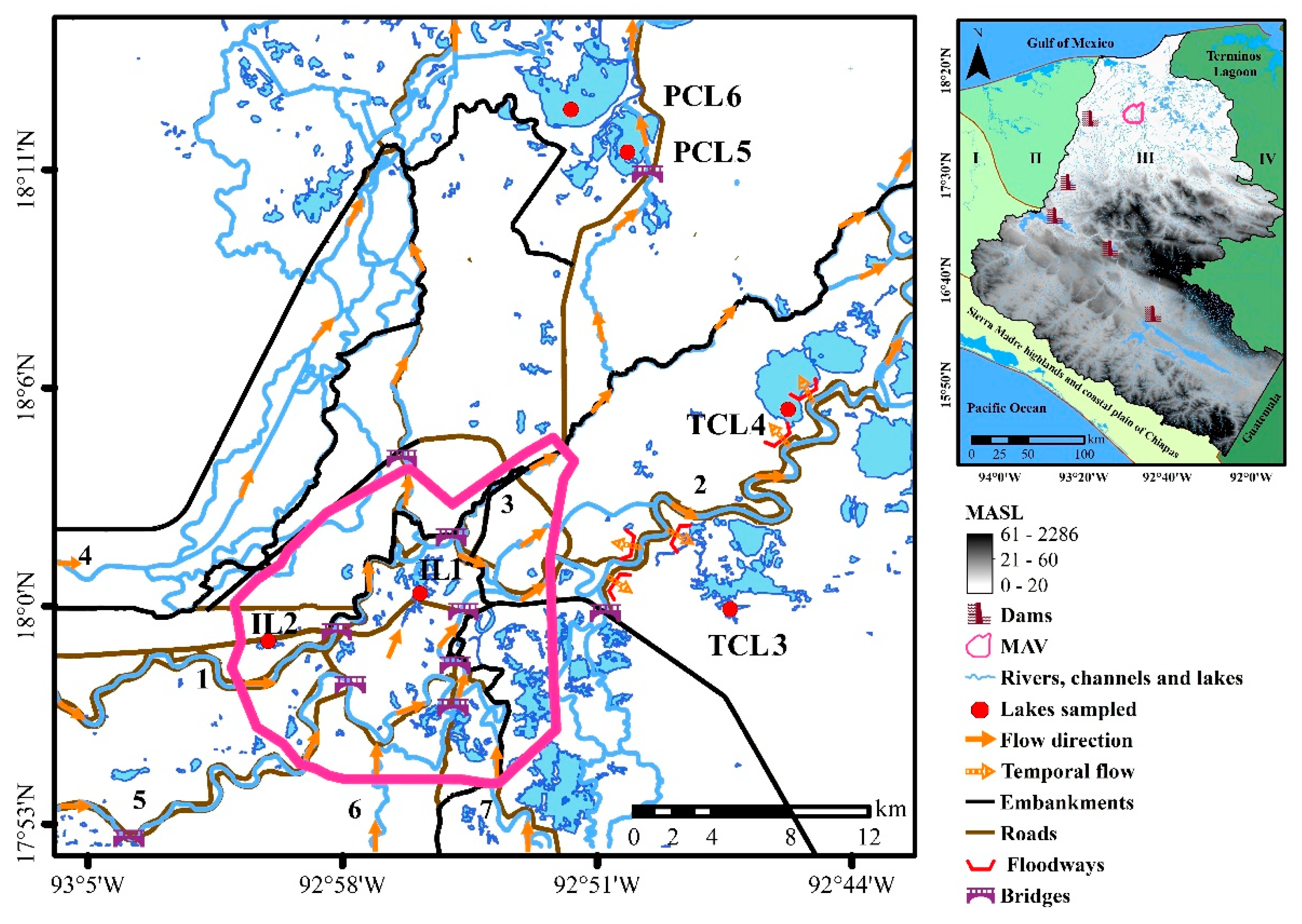
2.1. Study Area
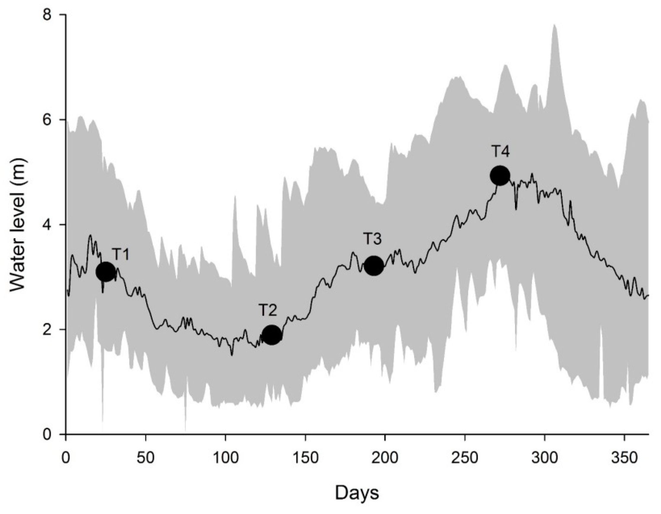
2.2. Sampling
2.3. Data Quality Control
2.4. Data Analysis
3. Results
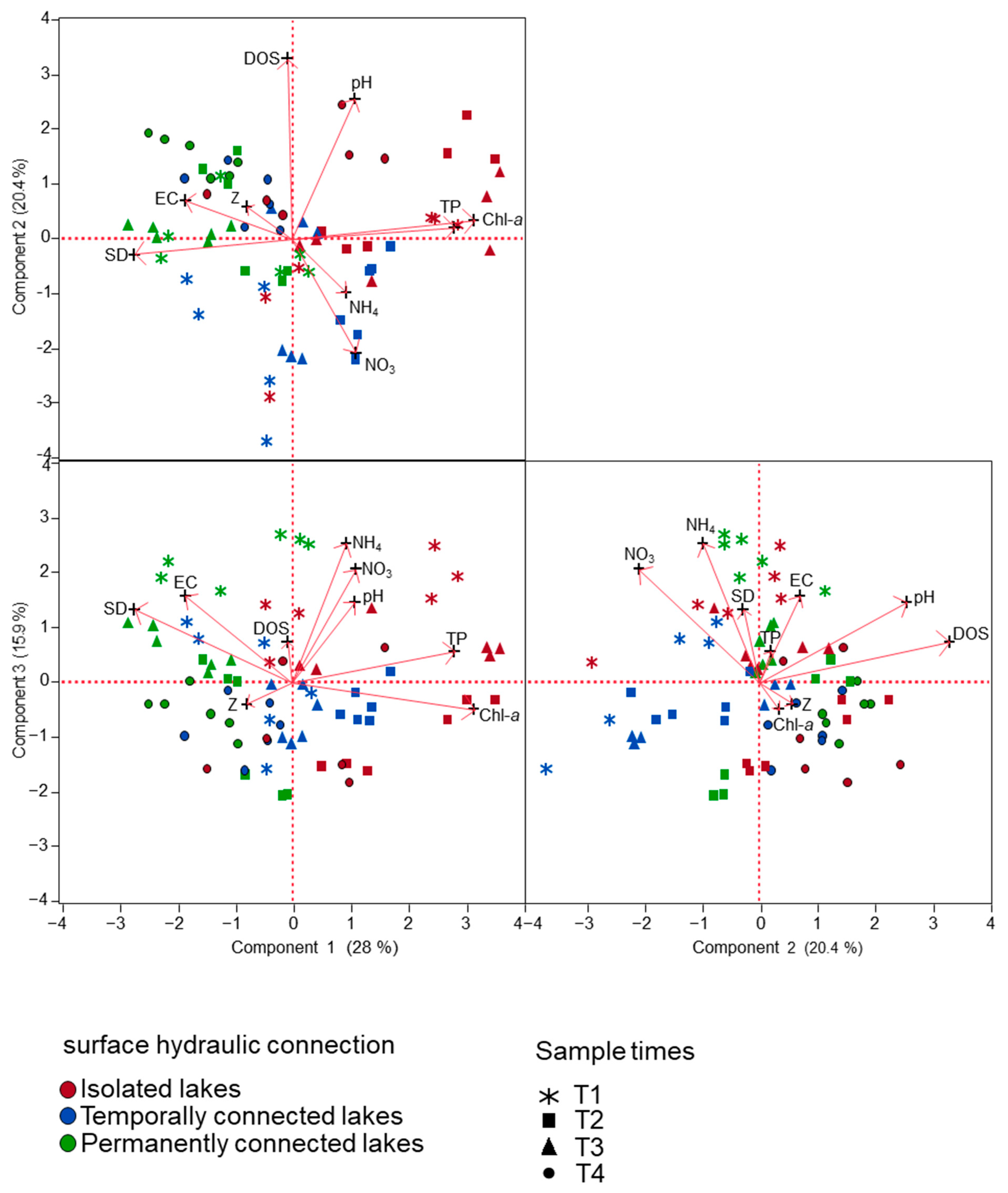
3.1. Spatial and Temporal Fluctuation of Environmental Variables
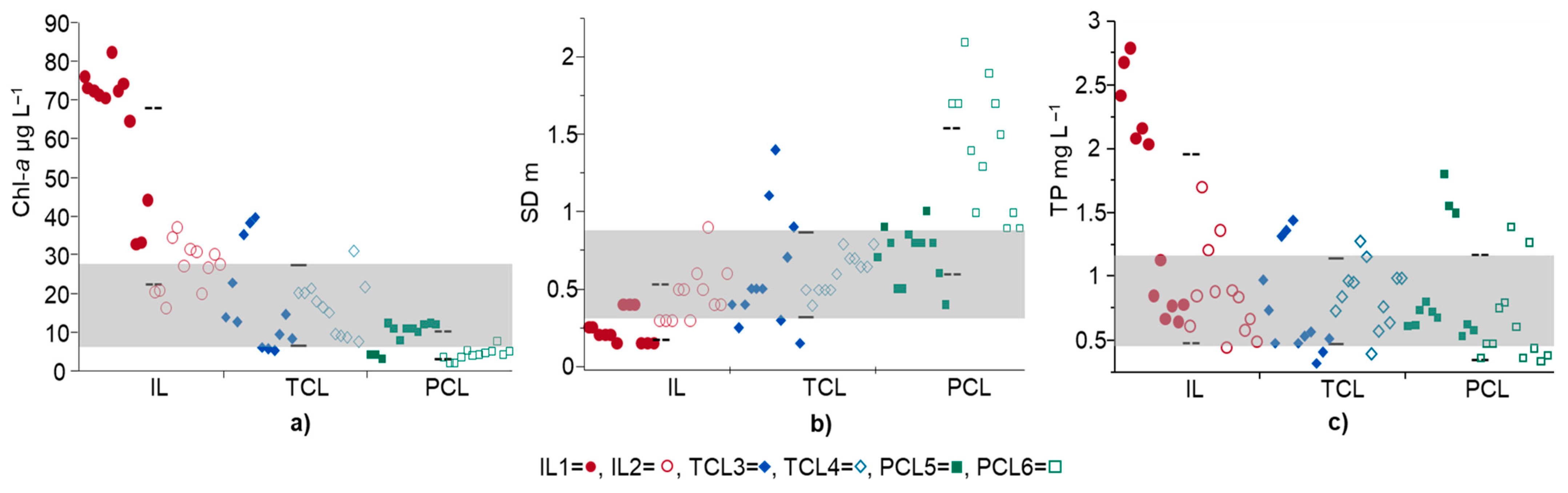
3.2. Overlapping of Water Quality Indicators under Three Surface Hydraulic Conditions
3.3. Trophic State under Different Surface Hydraulic Conditions
4. Discussion
4.1. Water Quality Indicators in Lakes with Different Surface Hydraulic Conditions
4.2. Overlapping of Water Quality Indicators in Three Surface Hydraulic Conditions
4.3. Variation of Trophic State Linked to Surface Hydraulic Conditions
5. Conclusions
Supplementary Materials
Author Contributions
Funding
Institutional Review Board Statement
Informed Consent Statement
Data Availability Statement
Acknowledgments
Conflicts of Interest
References
- Amoros, C.; Bornette, G. Connectivity and biocomplexity in waterbodies of riverine floodplains. Freshw. Biol. 2002, 47, 761–776. [Google Scholar] [CrossRef] [Green Version]
- Gurnell, A.M.; Rinaldi, M.; Belletti, B.; Bizzi, S.; Blamauer, B.; Braca, G.; Buijse, A.D.; Bussettini, M.; Camenen, B.; Comiti, F.; et al. A multiscale hierarchical framework for developing understanding of river behaviour to support river management. Aquat. Sci. 2016, 78, 1–16. [Google Scholar] [CrossRef] [Green Version]
- Shen, M.; Liu, X. Assessing the effects of lateral hydrological connectivity alteration on freshwater ecosystems: A meta-analysis. Ecol. Indic. 2021, 125, 107572. [Google Scholar] [CrossRef]
- Junk, W.J.; Bayley, P.B.; Sparks, R.E. The flood pulse concept in river-floodplain systems. In Proceedings of the International Large River Symposium, Honey Harbour, ON, Canada, 14 September 1986; Dodge, D.P., Ed.; Canadian Special Publication of Fisheries and Aquatic Sciences: Ontario, Canada, 1989; pp. 110–127. [Google Scholar]
- Racchetti, E.; Bartoli, M.; Soana, E.; Longhi, D.; Christian, R.R.; Pinardi, M.; Viaroli, P. Influence of hydrological connectivity of riverine wetlands on nitrogen removal via denitrification. Biogeochemistry 2011, 103, 335–354. [Google Scholar] [CrossRef]
- Jones, C.N.; Scott, D.T.; Edwards, B.L.; Keim, R.F. Perirheic mixing and biogeochemical processing in flow-through and backwater floodplain wetlands. Water Resour. Res. 2014, 50, 7394–7405. [Google Scholar] [CrossRef]
- Fritz, K.M.; Schofield, K.A.; Alexander, L.C.; McManus, M.G.; Golden, H.E.; Lane, C.R.; Kepner, W.G.; Le Duc, S.D.; DeMeester, J.E.; Pollard, A.I. Physical and chemical connectivity of streams and riparian wetlands to downstream waters: A synthesis. J. Am. Water Resour. As. 2018, 54, 323–345. [Google Scholar] [CrossRef]
- de Wilde, M.D.; Puijalon, S.; Vallier, F.; Bornette, G. Physico-chemical consequences of water-level decreases in wetlands. Wetlands 2015, 35, 683–694. [Google Scholar] [CrossRef]
- Cruz-Ramírez, A.K.; Salcedo, M.A.; Sánchez, A.J.; Barba Macías, E.; Mendoza Palacios, J.D. Relationship among physicochemical conditions, chlorophyll-a concentration, and water level in a tropical river–floodplain system. Int. J. Environ. Sci. Technol. 2019, 16, 3869–3876. [Google Scholar] [CrossRef]
- Larsen, L.G.; Harvey, J.W.; Maglio, M. Mechanisms of nutrient retention and its relation to flow connectivity in river–floodplain corridors. Freshw. Biol. 2015, 34, 187–205. [Google Scholar] [CrossRef]
- Park, E.; Latrubesse, E.M. The hydro-geomorphologic complexity of the lower Amazon River floodplain and hydrological connectivity assessed by remote sensing and field control. Remote Sens. Environ. 2017, 198, 321–332. [Google Scholar] [CrossRef]
- Li, Y.; Zhang, Q.; Cai, Y.; Tan, Z.; Wu, H.; Liu, X.; Yao, J. Hydrodynamic investigation of surface hydrological connectivity and its effects on the water quality of seasonal lakes: Insights from a complex floodplain setting (Poyang Lake, China). Sci. Total Environ. 2019, 660, 245–259. [Google Scholar] [CrossRef] [PubMed]
- Jones, C.N.; Scott, D.T.; Guth, C.R.; Hester, E.T.; Hession, W.C. Seasonal variation in floodplain biogeochemical processing in a restored headwater stream. Environ. Sci. Technol. 2015, 49, 13190–13198. [Google Scholar] [CrossRef] [PubMed]
- Sparks, R.E.; Blodgett, K.D.; Casper, A.F.; Hagy, H.M.; Lemke, M.J.; Velho, L.F.M.; Rodrigues, L.C. Why experiment with success? Opportunities and risks in applying assessment and adaptive management to the Emiquon floodplain restoration project. Hydrobiologia 2017, 804, 177–200. [Google Scholar] [CrossRef]
- Carlson, R.E.; Simpson, J. A Coordinator’s Guide to Volunteer Lake Monitoring Methods; North American Lake Management Society: Colorado Springs, CO, USA, 1996; p. 96. [Google Scholar]
- Jeppesen, E.; Brucet, S.; Naselli-Flores, L.; Papastergiadou, E.; Stefanidis, K.; Nõges, T.; Nõges, P.; Attayde, J.L.; Zohary, T.; Coppens, J.; et al. Ecological impacts of global warming and water abstraction on lakes and reservoirs due to changes in water level and related changes in salinity. Hydrobiologia 2015, 750, 201–227. [Google Scholar] [CrossRef]
- Thorp, J.H.; Thoms, M.C.; Delong, M.D. The riverine ecosystem synthesis: Biocomplexity in river networks across space and time. River Res. Appl. 2006, 22, 123–147. [Google Scholar] [CrossRef]
- Sánchez, A.J.; Salcedo, M.A.; Florido, R.; Mendoza, J.D.; Ruiz-Carrera, V.; Álvarez-Pliego, N. Ciclos de inundación y conservación de servicios ambientales en la cuenca baja de los ríos Grijalva-Usumacinta. ContactoS 2015, 97, 5–14. [Google Scholar]
- Zhang, Q.; Dong, X.; Chen, Y.; Yang, X.; Xu, M.; Davidson, T.A.; Jeppesen, E. Hydrological alterations as the major driver on environmental change in a floodplain Lake Poyang (China): Evidence from monitoring and sediment records. J. Great Lakes Res. 2018, 44, 377–387. [Google Scholar] [CrossRef]
- Poff, N.L.; Olden, J.D.; Merritt, D.M.; Pepin, D.M. Homogenization of regional river dynamics by dams and global biodiversity implications. Proc. Natl. Acad. Sci. USA 2007, 104, 5732–5737. [Google Scholar] [CrossRef] [Green Version]
- Poff, N.L.; Schmidt, J.C. How dams can go with the flow, small changes to water flow regimes from dams can help to restore river ecosystems. Science 2016, 353, 1099–1100. [Google Scholar] [CrossRef]
- Wolter, C.; Buijse, A.D.; Parasiewicz, P. Temporal and spatial patterns of fish response to hydromorphological processes. River Res. Appl. 2016, 32, 190–201. [Google Scholar] [CrossRef]
- Leira, M.; Cantonati, M. Effects of water-level fluctuations on lakes: An annotated bibliography. Hydrobiologia 2008, 613, 171–184. [Google Scholar] [CrossRef]
- Obolewski, K.; Glińska-Lewczuk, K.; Bąkowska, M. From isolation to connectivity: The effect of floodplain lake restoration on sediments as habitats for macroinvertebrate communities. Aquat. Sci. 2018, 80, 4. [Google Scholar] [CrossRef] [Green Version]
- Bunn, S.; Arthington, A.H. Basic principles and ecological consequences of altered flow regimes for aquatic biodiversity. Environ. Manag. 2002, 30, 492–500. [Google Scholar] [CrossRef] [PubMed] [Green Version]
- Dai, X.; Yang, G.; Wang, R.; Li, Y. The effect of the Changjiang River on water regimes of its tributary Lake East Dongting. J. Geogr. Sci. 2018, 28, 1072–1084. [Google Scholar] [CrossRef] [Green Version]
- Sánchez, A.J.; Salcedo, M.A.; Macossay-Córtez, A.A.; Feria-Díaz, Y.; Vázquez, L.; Ovando, N.; Rosado, L. Calidad ambiental de la laguna urbana La Pólvora en la cuenca del Río Grijalva. Tecnol. Cienc. Agua 2012, 3, 143–152. [Google Scholar]
- Cruz-Ramírez, A.K.; Salcedo, M.A.; Sánchez, A.J.; Mendoza Palacios, J.D.; Barba Macías, E.; Álvarez-Pliego, N.; Florido, R. Intra-annual variation of chlorophyll-a and nutrients in a hydraulically perturbed river-floodplain system in the Grijalva River basin. Hidrobiológica 2019, 29, 163–170. [Google Scholar] [CrossRef]
- Reckendorfer, W.; Funk, A.; Gschöpf, C.; Hein, T.; Schiemer, F. Aquatic ecosystem functions of an isolated floodplain and their implications for flood retention and management. J. Appl. Ecol. 2013, 50, 119–128. [Google Scholar] [CrossRef]
- Affonso, A.G.; Quieroz, H.L.; Novo, E.M.L.N. Abiotic variability among different aquatic systems of the central Amazon floodplain during drought and flood events. Braz. J. 2015, 75, 60–69. [Google Scholar] [CrossRef]
- Walalite, T.; Dekker, S.C.; Keizer, F.M.; Kardel, I.; Schot, P.P.; DeJong, S.M.; Wassen, M.J. Flood Water Hydrochemistry Patterns Suggest Floodplain Sink Function for Dissolved Solids from the Songkhram Monsoon River (Thailand). Wetlands 2016, 36, 995–1008. [Google Scholar] [CrossRef] [Green Version]
- Science for Environment Policy. Identifying Emerging Risks for Environmental Policies; Future Brief 13; Brief Produced for the European Commission DG Environment by the Science Communication Unit, UWE Bristol: Bristol, UK, 2016. [Google Scholar]
- Hidalgo, E.A.; Gómez, A.O.; Arreola, M.M. Manatees Mortality Analysis at Los Bitzales, Tabasco by Remote Sensing. Int. J. Latest Res. Eng. Technol. 2019, 5, 1–15. [Google Scholar]
- Ramos-Guajardo, A.B.; González-Rodríguez, G.; Colubi, A. Testing the degree of overlap for the expected value of random intervals. Int. J. Approx. Reason. 2020, 119, 1–19. [Google Scholar] [CrossRef]
- Zavala-Cruz, J.; Jiménez-Ramírez, R.; Palma-López, D.; Bautista-Zúñiga, F.; Gavi-Reyes, F. Paisajes geomorfológicos: Base para el levantamiento de suelos en Tabasco, México. Ecosist. Recur. Agropec. 2016, 3, 163–164. [Google Scholar] [CrossRef]
- Arreguín-Cortés, F.; Rubio-Gutiérrez, H.; Domínguez-Mora, R.; de Luna-Cruz, F. Análisis de las inundaciones en la planicie tabasqueña en el periodo 1995–2010. Tecnol. Cienc. Agua 2014, 5, 5–32. [Google Scholar]
- Palomeque de la Cruz, M.A.; Galindo, A.; Sánchez, A.J.; Escalona, M.J. Pérdida de humedales y vegetación por urbanización en la cuenca del Río Grijalva, México. Investig. Geogr. 2017, 68, 151–172. [Google Scholar] [CrossRef]
- Navarro, J.M.; Toledo, H. Transformación de la cuenca del Río Grijalva. Revista Noticias. Asoc. Mex. De Ing. Portuaria 2004, 4, 11–22. [Google Scholar]
- Comisión Nacional del Agua (CONAGUA). Atlas del Agua en México. 2018. Available online: http://sina.conagua.gob.mx/publicaciones/AAM_2018.pdf (accessed on 24 June 2018).
- Alcérreca-Huerta, J.C.; Callejas-Jiménez, M.E.; Carrillo, L.; Castillo, M.M. Dam implications on salt-water intrusion and land use within a tropical estuarine environment of the Gulf of Mexico. Sci. Total Environ. 2019, 652, 1102–1112. [Google Scholar] [CrossRef] [PubMed]
- Mendoza, A.; Soto-Cortés, G.; Priego-Hernández, G.; Rivera-Trejo, F. Historical description of the morphology and hydraulic behavior of a bifurcation in the lowlands of the Grijalva River Basin, Mexico. Catena 2019, 176, 343–351. [Google Scholar] [CrossRef]
- Sánchez, A.J.; Álvarez-Pliego, N.; Espinosa-Pérez, H.; Florido, R.; Macossay-Cortez, A.; Barba, E.; Salcedo, M.A.; Garrido-Mora, A. Species richness of urban and rural fish assemblages in the Grijalva Basin floodplain, southern Gulf of Mexico. Cybium 2019, 43, 239–254. [Google Scholar] [CrossRef]
- Instituto de Planeación y Desarrollo Urbano (IMPLAN). Programa de Desarrollo Urbano del Centro de Población de la Ciudad de Villahermosa y Centros Metropolitanos del Municipio de Centro, Tabasco 2008–2030. 2008. Available online: https://tabasco.gob.mx/programas-de-desarrollo-urbano-municipios. (accessed on 15 April 2016).
- Instituto Nacional de Estadística y Geografía (INEGI). Delimitación de las Zonas Metropolitanas de México 2015. 2018. Available online: https://www.gob.mx/conapo/documentos/delimitacion-de-las-zonas-metropolitanas-de-mexico-2015. (accessed on 12 May 2019).
- Instituto Nacional de Estadística y Geografía (INEGI). Simulador de Flujos de Agua de Cuencas Hidrográficas Versión 4.0. 2021. Available online: https://antares.inegi.org.mx/analisis/red_hidro/siatl/. (accessed on 12 April 2021).
- Salcedo, M.A.; Sánchez, A.J.; Cruz-Ramírez, A.K.; Álvarez-Pliego, N.; Florido, R.; Ruiz-Carrera, V.; Garrido, A.; Alejo-Díaz, R. Aplicación del índice de calidad del agua (WQI-NSF) en lagunas metropolitanas y rurales. Agroproductividad 2018, 11, 81–86. [Google Scholar]
- Comisión Nacional del Agua (CONAGUA). Banco Nacional de Datos de Aguas Superficiales. 2016. Available online: http://app.conagua.gob.mx/bandas/ (accessed on 12 May 2016).
- Carlson, R.E. A trophic state index for lakes. Limnol. Oceanogr. 1977, 22, 361–369. [Google Scholar] [CrossRef] [Green Version]
- Rocha, R.R.A.; Thomaz, S.M.; Carvalho, P.; Gomes, L.C. Modeling chlorophyll-a and dissolved oxygen concentration in tropical floodplain lakes (Paraná River, Brazil). Braz. J. Biol. 2009, 69, 491–500. [Google Scholar] [CrossRef] [PubMed] [Green Version]
- Zhang, Y.; Yang, G.; Li, B.; Cai, Y.; Chen, Y. Using eutrophication and ecological indicators to assess ecosystem condition in Poyang Lake, a Yangtze-connected lake. Aquat. Ecosyst. Health 2016, 19, 29–39. [Google Scholar] [CrossRef]
- Uzarski, D.G.; Wilcox, D.A.; Brady, V.J.; Cooper, M.J.; Albert, D.A.; Ciborowski, J.J.H.; Danz, N.P.; Garwood, A.; Gathman, J.P.; Thomas, M.G.; et al. Leveraging a Landscape-Level Monitoring and Assessment Program for Developing Resilient Shorelines throughout the Laurentian Great Lakes. Wetlands 2019, 39, 1357–1366. [Google Scholar] [CrossRef] [Green Version]
- American Public Health Association (APHA). Standard Methods for the Examination of Water and Wastewater; American Public Health Association, American Water Works Association, Water Environment Federation: Washington, DC, USA, 1998. [Google Scholar]
- Zar, J.H. Biostatistical Analysis, 5th ed.; Prentice Hall: Englewood Cliffs, NJ, USA, 2010; ISBN 978-0-13-100846-5. [Google Scholar]
- Diamantini, E.; Lutz, S.R.; Mallucci, S.; Majone, B.; Merz, R.; Bellin, A. Driver detection of water quality trends in three large European river basins. Sci. Total Environ. 2018, 612, 49–62. [Google Scholar] [CrossRef]
- Yang, K.; Yu, Z.; Luo, Y.; Yang, Y.; Zhao, L.; Zhou, X. Spatial and temporal variations in the relationship between lake water surface temperatures and water quality—A case study of Dianchi Lake. Sci. Total Environ. 2018, 624, 859–871. [Google Scholar] [CrossRef]
- Weilhoefer, C.L.; Yangdong, P.; Eppard, S. The effects of river floodwaters on floodplain wetland water quality and diatom assemblages. Wetlands 2008, 28, 473–486. [Google Scholar] [CrossRef]
- Legendre, P.; Legendre, L. Numerical Ecology, 2nd ed.; Elsevier: Amsterdam, The Netherlands, 2003; ISBN 0-444-89250-8. [Google Scholar]
- Mohammed, M.B.; Adam, M.B.; Zulkafli, H.S.; Ali, N. Improved Frequency Table with Application to Environmental Data. Math. Stat. 2020, 8, 201–210. [Google Scholar] [CrossRef]
- Carlson, R.E.; Havens, K.E. Simple graphical methods for the interpretation of relationships between trophic state variables. Lake Reserv. Manag. 2005, 21, 107–118. [Google Scholar] [CrossRef]
- Yuan, Y.; Jiang, M.; Liu, X.; Yu, H.; Otte, M.L.; Ma, C.; Her, Y.G. Environmental variables influencing phytoplankton communities in hydrologically connected aquatic habitats in the Lake Xingkai basin. Ecol. Indic. 2018, 91, 1–12. [Google Scholar] [CrossRef]
- Liu, X.; Qian, K.; Chen, Y.; Gao, J.A. comparison of factors influencing the summer phytoplankton biomass in China’s three largest freshwater lakes: Poyang, Dongting, and Taihu. Hydrobiologia 2017, 792, 283–302. [Google Scholar] [CrossRef]
- Wetzel, R.G. Limnology Lake and River Ecosystems, 3rd ed.; Academic Press: San Diego, CA, USA, 2001; ISBN 10: 0-12-744760-1. [Google Scholar]
- Scheffer, M. Ecology of Shallow Lakes; Chapman and Hall: London, UK, 1998; ISBN 9780412749209. [Google Scholar]
- Blottière, L.; Jaffar-Bandjee, M.; Jacquet, S.; Millot, A.; Hulot, F.D. Effect of mixing on the pelagic food web in shallow lakes. Freshw. Biol. 2017, 62, 161–177. [Google Scholar] [CrossRef]
- Vymazal, J. Removal of nutrients in various types of constructed wetlands. Sci. Total Environ. 2007, 380, 48–65. [Google Scholar] [CrossRef] [PubMed]
- Pinilla, G. An index of limnological conditions for urban wetlands of Bogota city, Colombia. Ecol. Indic. 2010, 10, 848–856. [Google Scholar] [CrossRef]
- Andersen, T.K.; Nielsen, A.; Jeppesen, E.; Hu, F.; Bolding, K.; Liu, Z.; Søndergaard, M.L.S.; Johansson, L.S.; Trolle, D. Predicting ecosystem state changes in shallow lakes using an aquatic ecosystem model: Lake Hinge, Denmark, an example. Ecol. Appl. 2020, 30, e02160. [Google Scholar] [CrossRef] [PubMed]
- Balan, A.; Obolewski, A.; Luca, M.; Cretescu, U. Use of macroinvertebrates for assessment of restoration works influence on the habitat in floodplain lakes. Environ. Eng. Manag. J. 2017, 16, 969–978. [Google Scholar] [CrossRef]
- Szpakowska, B.; Świerk, D.; Pajchrowska, M.; Gołdyn, R. Verifying the usefulness of macrophytes as an indicator of the status of small waterbodies. Sci. Total Environ. 2021, 798, 149279. [Google Scholar] [CrossRef]
- Zhu, Q.D.; Sun, J.H.; Hua, G.F.; Wang, J.H.; Wang, H. Runoff characteristics and non-point source pollution analysis in the Taihu Lake Basin: A case study of the town of Xueyan, China. Environ. Sci. Pollut. Res. 2015, 22, 15029–15036. [Google Scholar] [CrossRef]
- Cowardin, L.M.; Carter, V.; Golet, F.C.; LaRoe, E.T. Classification of Wetlands and Deepwater Habitats of the United States; US Department of the Interior, US, Fish and Wildlife Service: Washington, DC, USA, 1979. [Google Scholar]
- Xu, F.L.; Jiao, Y. Trophic classification for lakes. In Encyclopedia of Ecology, 2nd ed.; Fath, B., Ed.; Elsevier: Amsterdam, The Netherlands, 2019; ISBN 9780444641304. [Google Scholar]
- Zou, W.; Zhu, G.; Cai, Y.; Vilmi, A.; Xu, H.; Zhu, M.; Gong, Z.; Zhang, Y.; Qin, B. Relationships between nutrient, chlorophyll a and Secchi depth in lakes of the Chinese Eastern Plains ecoregion: Implications for eutrophication management. J. Environ. Manag. 2020, 260, 1–9. [Google Scholar] [CrossRef]
- Ren, J.; Zheng, Z.; Li, Y.; Lv, G.; Wuang, Q.; Lyu, H.; Huang, C.; Liu, G.; Du, C.; Mu, M.; et al. Remote observation of water clarity patterns in Three Gorges Reservoir and Dongting Lake of China and their probable linkage to the Three Gorges Dam based on Landsat 8 imagery. Sci. Total Environ. 2018, 625, 1554–1566. [Google Scholar] [CrossRef]
- Carhart, A.M.; Kalas, J.E.; Rogala, J.T.; Rohweder, J.J.; Drake, D.C.; Houser, J.N. Understanding constraints on submersed vegetation distribution in a large, floodplain river: The role of water level fluctuations, water clarity and river geomorphology. Wetlands 2021, 41, 1–15. [Google Scholar] [CrossRef]
- Sheela, A.M.; Letha, J.; Joseph, S. Environmental status of a tropical lake system. Environ. Monit. Assess. 2011, 180, 427–449. [Google Scholar] [CrossRef] [PubMed]
- de Amo, V.E.; Ernandes-Silva, J.; Moi, D.A.; Mormul, R.P. Hydrological connectivity drives the propagule pressure of Limnoperna fortunei (Dunker, 1857) in a tropical river–floodplain system. Hydrobiologia 2021, 848, 2043–2053. [Google Scholar] [CrossRef]
- Wu, P.; Qin, B.; Yu, G. Estimates of long-term water total phosphorus (TP) concentrations in three large shallow lakes in the Yangtze River basin, China. Environ. Sci. Pollut. Res. 2016, 23, 4938–4948. [Google Scholar] [CrossRef] [PubMed]
- Wang, Y.; Molinos, J.G.; Shi, L.; Zhang, M.; Wu, Z.; Zhang, H.; Xu, J. Drivers and Changes of the Poyang Lake Wetland Ecosystem. Wetlands 2019, 39, 35–44. [Google Scholar] [CrossRef]
- Schallenberg, M.; Burns, C.W. Effects of sediment resuspension on phytoplankton production: Teasing apart the influences of light, nutrients and algal entrainment. Freshw. Biol. 2004, 49, 143–159. [Google Scholar] [CrossRef]
- Lázaro-Vázquez, A.; Castillo, M.M.; Jarquín-Sánchez, A.; Carrillo, A.L.; Capps, K.A. Temporal changes in the hydrology and nutrient concentrations of a large tropical river: Anthropogenic influence in the Lower Grijalva River, Mexico. River. Res. Appl. 2018, 34, 649–660. [Google Scholar] [CrossRef]
- Goñi-Arévalo, J.A.; Hernández-Pérez, O.; Toledo-Gómez, J.L.; Pérez Méndez, M.A. Eutroficación de la laguna de las Ilusiones y un modelo empírico de fósforo. Universidad y Ciencia 1991, 8, 47–53. [Google Scholar]
- Hettiarachchi, M.; Morrison, T.H.; Wickramsinghe, D.; Mapa, R.; De Alwis, A.; McAlpine, C.A. The eco-social transformation of urban wetlands: A case study of Colombo, Sri Lanka. Landsc. Urban Plan. 2014, 132, 55–68. [Google Scholar] [CrossRef]
- Sánchez, A.J.; Florido, R.; Salcedo, M.A.; Ruiz-Carrera, V.; Montalvo-Urgel, H.; Raz-Guzmán, A. Macrofaunistic diversity in Vallisneria americana Michx. in a tropical wetland, Southern Gulf of Mexico. In Ecosystems I.; Mahamane, A., Ed.; InTech: Rijeka, Croatia, 2012; pp. 1–26. ISBN 978-953-51-5289-7. [Google Scholar]
- Lone, P.A.; Bhardwaj, A.K.; Shah, K.W. Macrophytes as powerful natural tools for water quality improvement. Res. J. Bot. 2014, 9, 24–30. [Google Scholar] [CrossRef] [Green Version]
- Thoms, M.C. Floodplain–river ecosystems: Lateral connections and the implications of human interference. Geomorphology 2003, 56, 335–349. [Google Scholar] [CrossRef]
- Biswas, S.S.; Pani, P. Changes in the hydrological regime and channel morphology as the effects of dams and bridges in the Barakar River, India. Environ. Earth Sci. 2021, 80, 1–18. [Google Scholar] [CrossRef]
- Zhang, P.; Zhang, H.; Wang, H.; Hilt, S.; Li, C.; Yu, C.; Zhang, M.; Xu, J. Warming alters juvenile carp effects on macrophytes resulting in a shift to turbid conditions in freshwater mesocosms. J. Appl. Ecol. 2022, 59, 165–175. [Google Scholar] [CrossRef]
- Weigelhofer, G.; Preiner, S.; Fun, A.; Bondar-Kunze, E.; Hein, T. The hydrochemical response of small and shallow floodplain water bodies to temporary surface water connections with the main river. Freshw. Biol. 2015, 60, 781–793. [Google Scholar] [CrossRef]
- Moorman, M.C.; Augspurger, T.; Stanton, J.D.; Smith, A. Where’s the Grass? Disappearing Submerged Aquatic Vegetation and Declining Water Quality in Lake Mattamuskeet. J. Fish Wildl. Manag. 2016, 8, 401–417. [Google Scholar] [CrossRef]


| Chl-a | SD | TP | |||||||
|---|---|---|---|---|---|---|---|---|---|
| µg L−1 | m | mg L−1 | |||||||
| IL | TCL | PCL | IL | TCL | PCL | IL | TCL | PCL | |
| Recorded overlapping sites | 7 | 17 | 10 | 14 | 19 | 13 | 14 | 16 | 14 |
| Proportion of overlapping sites | 0.41 | - | 0.59 | 0.74 | - | 0.68 | 0.88 | - | 0.88 |
| Reference intervals ( ± SD) (RITCL) | - | 6.8–27.4 | - | - | 0.3–0.9 | - | - | 0.48–1.14 | - |
| Class size of TLC (CS) | 20.6 | 0.6 | 0.66 | ||||||
| Overlap intervals | 16.2–27.3 | - | 7.7–22.6 | 0.3–0.6 | - | 0.3–0.9 | 0.49–1.12 | - | 0.48–0.8 |
| Overlap size (OS) | 11.1 | 14.9 | 0.3 | 0.6 | 0.63 | 0.32 | |||
| Proportionality overlap (PO) | 0.54 | - | 0.72 | 0.50 | - | 1.0 | 0.95 | - | 0.48 |
| Trophic state | E | E | E | H | E | E | H | H | H |
| Variables | PCI | PC2 | PC3 |
|---|---|---|---|
| WL | −0.136 | 0.120 | −0.089 |
| SD | −0.478 | −0.055 | 0.313 |
| DOS | −0.013 | 0.677 | 0.176 |
| EC | −0.323 | 0.146 | 0.368 |
| pH | 0.190 | 0.525 | 0.343 |
| TP | 0.493 | 0.043 | 0.134 |
| NH4+ | 0.164 | −0.200 | 0.590 |
| NO3− | 0.193 | −0.424 | 0.481 |
| Chl-a | 0.553 | 0.073 | −0.113 |
| Eigenvalue | 2.521 | 1.834 | 1.428 |
| Explained variance (%) | 28.0 | 20.4 | 15.9 |
| Accumulated variance (%) | 28.0 | 48.4 | 64.2 |
Publisher’s Note: MDPI stays neutral with regard to jurisdictional claims in published maps and institutional affiliations. |
© 2022 by the authors. Licensee MDPI, Basel, Switzerland. This article is an open access article distributed under the terms and conditions of the Creative Commons Attribution (CC BY) license (https://creativecommons.org/licenses/by/4.0/).
Share and Cite
Salcedo, M.Á.; Cruz-Ramírez, A.K.; Sánchez, A.J.; Álvarez-Pliego, N.; Florido, R.; Ruiz-Carrera, V.; Morales-Cuetos, S.S. Water Quality Indicators in Three Surface Hydraulic Connection Conditions in Tropical Floodplain Lakes. Water 2022, 14, 3931. https://doi.org/10.3390/w14233931
Salcedo MÁ, Cruz-Ramírez AK, Sánchez AJ, Álvarez-Pliego N, Florido R, Ruiz-Carrera V, Morales-Cuetos SS. Water Quality Indicators in Three Surface Hydraulic Connection Conditions in Tropical Floodplain Lakes. Water. 2022; 14(23):3931. https://doi.org/10.3390/w14233931
Chicago/Turabian StyleSalcedo, Miguel Ángel, Allan Keith Cruz-Ramírez, Alberto J. Sánchez, Nicolás Álvarez-Pliego, Rosa Florido, Violeta Ruiz-Carrera, and Sara Susana Morales-Cuetos. 2022. "Water Quality Indicators in Three Surface Hydraulic Connection Conditions in Tropical Floodplain Lakes" Water 14, no. 23: 3931. https://doi.org/10.3390/w14233931