Daily Streamflow Time Series Modeling by Using a Periodic Autoregressive Model (ARMA) Based on Fuzzy Clustering

Abstract

The behavior of hydrological processes is periodic and stochastic due to the influence of climatic factors. Therefore, it is crucial to develop the models based on their periodicity and stochastic nature for prediction. Furthermore, forecasting the streamflow, as one of the main components of the hydrological cycle, is a primary subject. In this study, a statistical method, Fuzzy C-means clustering, was used to find the periodicity in the daily discharge time series, whereas autoregressive moving average, ARMA, was used in modeling every cluster. Dividing the daily stream flow time series into smaller groups based on their similar statistical behavior by using a statistical method for analyzing and a combination of Fuzzy C-means clustering and ARMA modeling is the innovation of this study. We draw on the daily discharge data of four different river stations in Hesse state in Germany. The collected data cover 18 years, from 2000 to 2017. Root mean square error (RMSE) was used to evaluate the accuracy. The results revealed that the performance of ARMA in four stations for predicting every cluster was reliable. In addition, it must be highlighted that by clustering the daily stream flow time series into smaller groups, forecasting different days of the year will be possible.

1. Introduction

In the current world, water resources management plays an increasingly important role. Although 70 percent of the earth’s surface is covered by water, the problem is that sometimes it is too much or too little, and it is occasionally costly or polluted. On the other hand, not only is consuming water increasing all around the world due to population growth, land use change, and upgrading life standards [1], but also the negative direct impact of climate change on water resources and freshwater ecosystems has restricted them and put the world at the risk of losing some water resources [2]. It can be said that managing water resources has been one of the biggest challenges in all countries for the past decades, which has necessitated the use of innovative tools such as advanced statistical methods and data mining for management, planning, and policy in the field of water resources.

Data mining has been recognized as one of the most useful and powerful tools among the various sciences for analyzing high-volume data and large databases; finding the unknown relationship between the data and using this knowledge has increased significantly in the last decades [3,4,5,6,7]. Data mining means discovering knowledge and extracting useful information from a large amount of raw data. Various international scientific centers are using this important issue to prepare the information necessary for policymakers, planners, and managers to make decisions. Furthermore, data mining is a procedure to divide the data into groups according to their type, discover the behavior of the groups and check the correlation between them, and research the scientific issues; there has been growth in using it in recent years. Liu et al. proved the capability of data mining for analyzing data compared to conventional methods. They showed that by using data mining, the efficiency of material data analysis could go up by 10% [8]. Data mining techniques have played a large role in water resources management as an exploratory process. In this regard, the following are some examples:

A data mining approach is used as part of an integrated water management model to describe and simulate farmers’ decision rules in a catchment in northern Thailand [9]. Investigation of water resources data for quality and quantity time series [10] and promising likelihoods streamflow forecast models for river/reservoir systems and nonlinearity of climate teleconnections dynamics [11] are two other types of research in this field. Furthermore, finding the dependency of monthly precipitation of some synoptic stations and eliminating the trend of surface temperature with the help of data mining is another example [12].

Among the methods of data mining, the Fuzzy cluster is a method that divides the data into groups with similar items. It can be considered a data modeling technique that briefly explains the data. Therefore, data mining can be applied to a wide range of subjects [13]. Luczak et al. [14] specified the time of transaction of the COVID-19 epidemic between the European countries and followed the continuous changes during the transaction using the Fuzzy cluster method. They recognized the countries’ COVID-19 epidemic state in Europe in this research. The simplicity and efficiency of the Fuzzy clustering method are mentioned in Zhang et al. [15]. They have mentioned an improved Fuzzy clustering method for image segmentation in medical images, which is useful for judgment about illnesses based on nonlocal self-similarity and a prior low rank. The results showed that by utilizing this new approach, results would be valuable and acceptable.

In addition, using this method in water resources research has increased dramatically. The effective impact of using clustering analysis for estimating failure rate in water distribution networks and determining the relationship between failure-rate-effective factors has been acknowledged [16]. Using clustering to divide gauged and ungauged watersheds into homogenous groups based on a variety of topographical and climatic factors shows another application of clustering in water resource management [17]. Identification of hydrologically homogeneous regions to estimate the regional flood index was done by using the clustering method [18]. In another study, clustering has been the main method for describing and classifying the potential water resources availability (PWRA) distributed over an area [19]. Furthermore, the relationship between groundwater resources and surface waters was investigated by cluster analysis [20].

Periodic time series are often used for modeling climatological data, hydrology, economics, electricity, engineering, etc. As a natural phenomenon, water flow behavior repeats over fixed time intervals, so periodic data should be considered [21]. Research in periodic time series has been done by researchers [22,23,24,25,26], and generally, it can be found that periodic hydrology time series, such as seasonal, monthly, weekly, and daily stream flow time series, have periodic and random features. Periodic features are defined by periodic average, standard deviation, and periodic skewness coefficient; constant or periodic correlation coefficient may indicate random features. A wide spectrum of techniques can model the time series once a periodic pattern has been discovered, improving the prediction [27].

To our knowledge, no previous studies have investigated on deviation of the daily discharge of these four stations studied in this research into groups according to their behavior. This study uses the Fuzzy clustering method to find the periodicity based on the days with similar statistical behavior, not based on calendar divisions such as month or season. In addition, the suitability of ARMA (autoregressive moving average), a short-memory powerful linear model, to model daily river discharge will be investigated. Our proposed method realizes the principle of parsimony in modeling and reduces the estimation of periodic parameters. Additionally, this method will divide time series into smaller groups, and the linear features of any groups will be improved. Therefore, using ARMA (autoregressive moving average) models can have more accurate results. Policymakers and local authorities can use the results of this study to reduce the manageable damages caused by hydrological events by planning ahead.

After the introduction, the study region, preparation of data, and methodology (Section 2) are presented, followed by the results in Section 3. The discussion is in Section 4. Finally, the conclusions and outlook have been placed in the last section.

2. Materials and Methods

2.1. Study Site

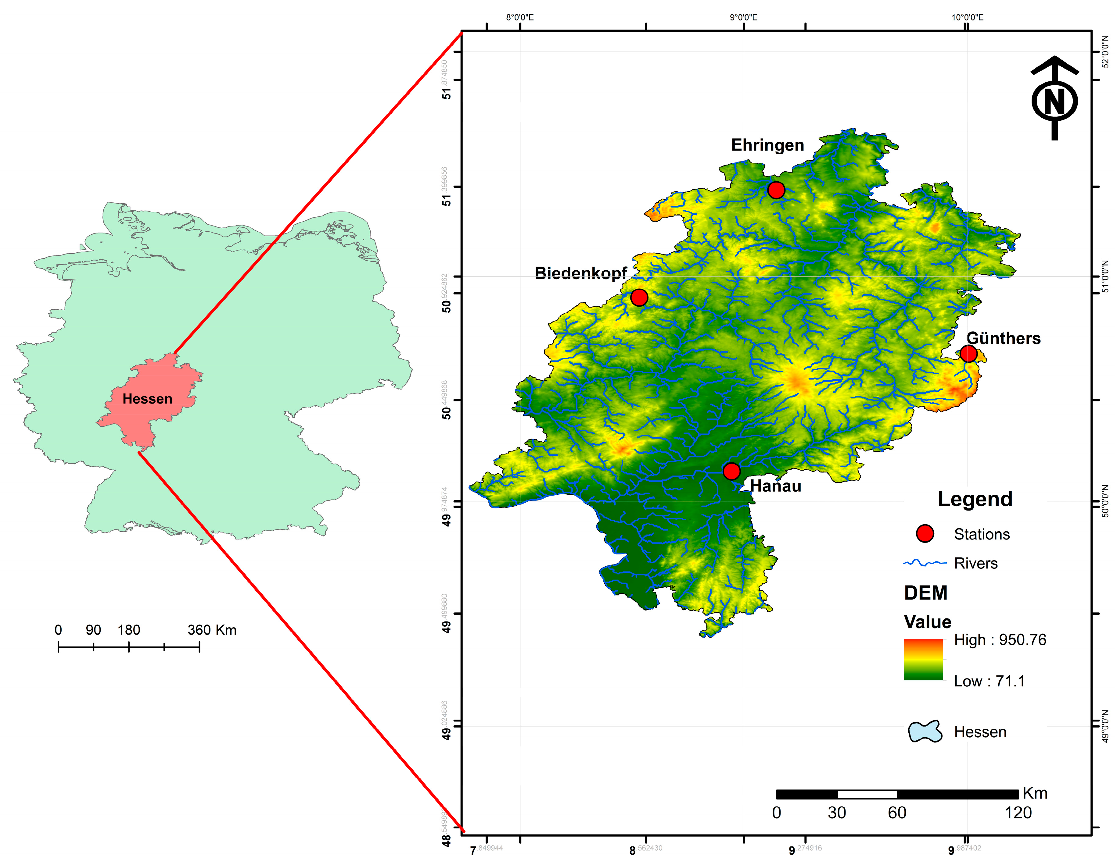
Located in the heart of Europe, Germany has a total area of 357,588 km² with 53.5% agricultural land, 29.5% wood and forest, 12.5% city and traffic areas, 1.8% water, and 2.4% other land uses [28]. The Hesse area (21,116 km²) is located in Germany, with the highest and lowest elevations of 950 and 71 m asl, respectively [28]. According to the German Weather Service, the climate is classified as temperate oceanic, with a mean annual air temperature of 9.3 °C and mean annual precipitation of 790 mm (1991–2020) [29]. The selected state gauges Ehringen (lat = 51.38367, lon = 9.14531, catchment area = 137 km²), Hanau (lat = 50.13208, lon = 8.94581, catchment area = 920 km²), Biedenkopf (lat = 50.90598, lon = 8.53263, catchment area = 303 km²), and Günthers (lat = 50.65609, lon = 10.00497, catchment area = 182 km²) are located on four main rivers, namely, the Erpe, Kinzig, Lahn, and Ulster, respectively [30]. The Erpe is a tributary of the Twiste and belongs to the Weser river system. It has its source in the low mountain range Habichtswald in northern Hesse [31]. The Kinzig river runs along the northern lowlands and lower mountains of Germany’s central lower mountainous region [32]. The Lahn river originates in the Rothaar Mountains in North Rhine-Westphalia and flows into the Rhine at Lahnstein, near Koblenz (Rhineland-Palatinate). The Lahn measures approximately 245 km in length [33]. The Fulda and Ulster rivers drain Eastern Hesse almost entirely. The Weser’s second headstream, the Ulster, is a principal tributary of the Werra river. A source of the Ulster river can be found in the southeast of the study area near the highest peaks of the Rhön Mountains [34]. Figure 1. shows an overview of the study site in this study.

2.2. Database

2.2.1. Description

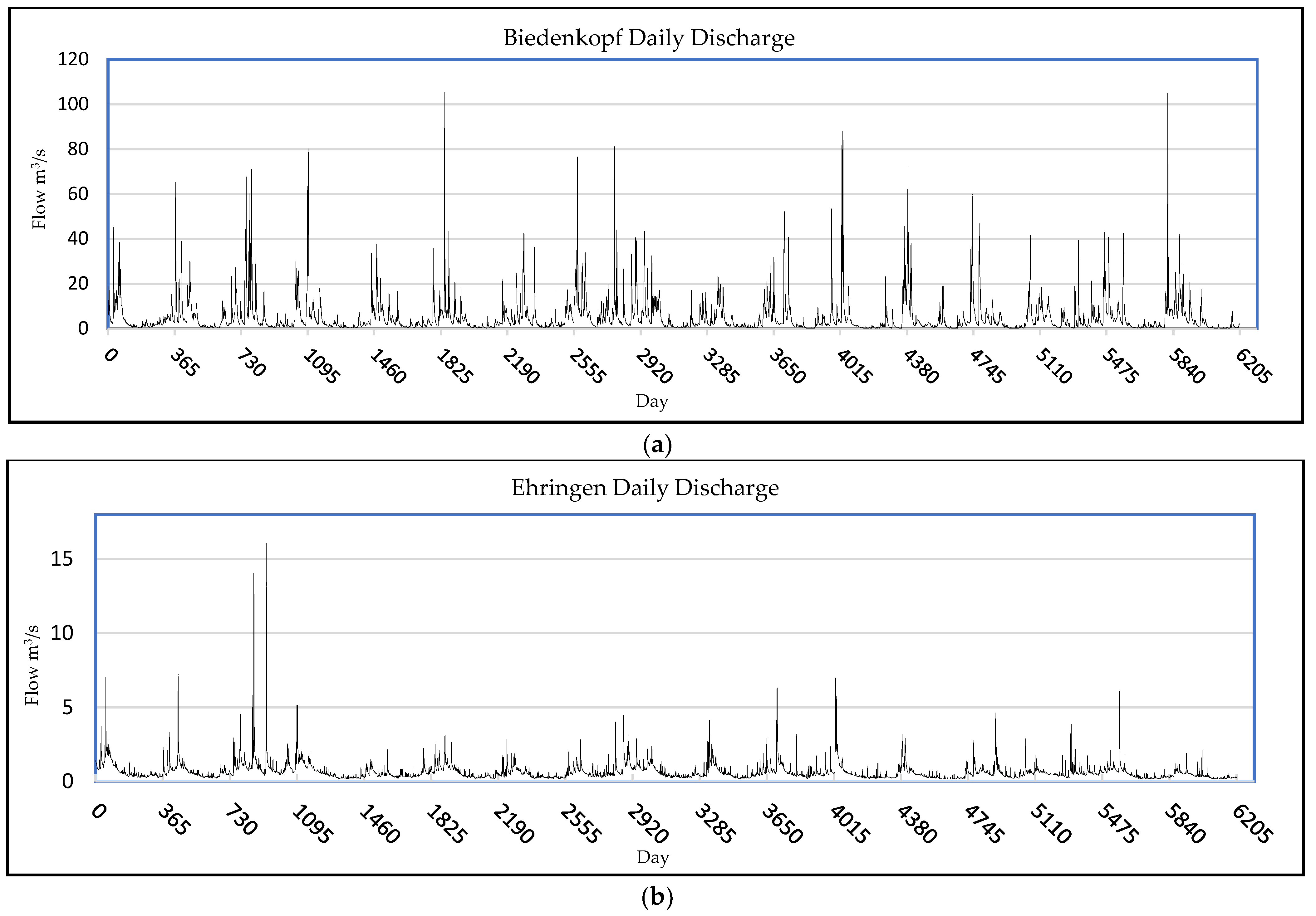
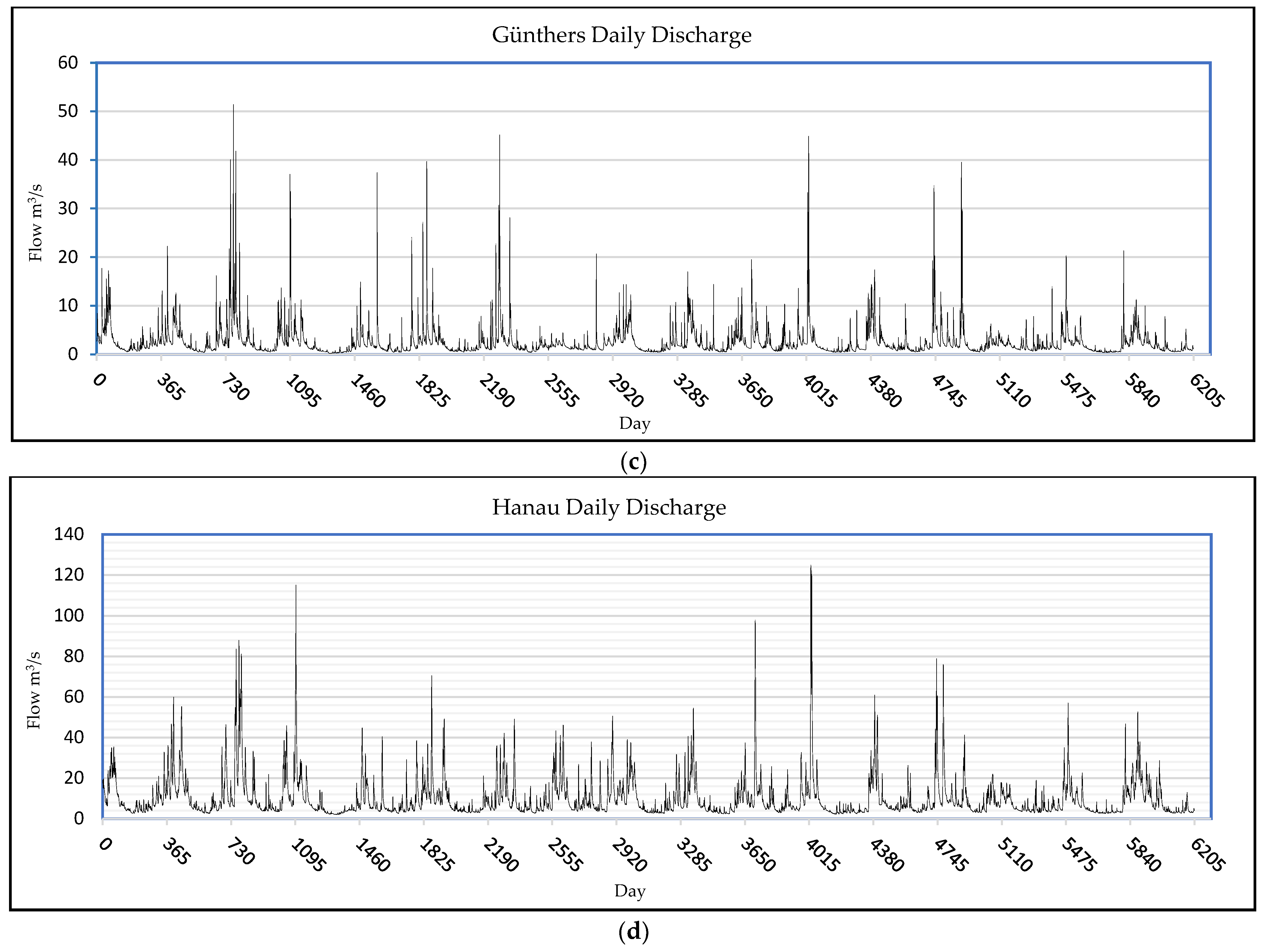
In this study, four measurement stations, including Ehringen, Hanau, Biedenkopf, and Günthers, which provide the daily flow of the rivers, have been used to develop the model. Figure 2a–d represent the daily discharge of the stations. In accordance with the situations of being on various hydrological conditions, the stations were chosen randomly in Hesse’s four main geographical regions: North, South, East, and West. The data were collected from the Hessian Agency for Nature Conservation, Environment, and Geology (HLNUG), https://www.hlnug.de/static/pegel/wiskiweb2/ (accessed on 20 October 2022). As a technical and scientific authority within the Hessian environmental administration, the HLNUG is responsible for environmental monitoring. An area-wide monitoring network records air pollutants and physical, chemical, and biological water and soil parameters. In addition to data recording, the main tasks include collecting, processing, and evaluating such data. For this study, a unified length of time series was set, and the starting and ending date is from January 2000 to December 2017, respectively. Figure 2 shows the graphs of the data sets. Based on Figure 2, 2002 is the year with the maximum average daily discharge for the stations Ehringen, Hanau, and Günthers, whereas for Biedenkopf station, the maximum average daily discharge was in 2007. On the other hand, the minimum daily discharge for the stations happened in 2016 for Ehringen and Biedenkopf, in 2014 for Hanau, and in 2007 for Günthers.

Table 1. Summary of descriptive statistics of daily discharge for four stations.

Station	Period	Samples	Average (m3/s)	Standard Deviation (m3/s)	Skewness (m3/s)	Kurtosis (m3/s)
Biedenkopf	2000–2017	6570	5.11	7.91	4.24	27.38
Ehringen	2000–2017	6570	0.64	0.59	7.57	128.89
Günthers	2000–2017	6570	2.56	3.29	5.51	47.01
Hanau	2000–2017	6570	9.91	10.20	3.55	19.65

summarizes more details regarding the data.

2.2.2. Preprocessing

The forecast package in R programming has done all the data processing procedures, including normalization and removing nonstationary factors and outliers. It is worth mentioning that there were no data gaps or missing values due to the data checking and preparation by the HLNUG. Therefore, in the first step, we stabled variance and normalized the data using Box–Cox transformation. Then, for omitting the seasonality, the data has been standardized and checked for the stationary using an augmented Dickey–Fuller Test (ADF). Therefore, they will be ready for clustering and modeling.

2.3. Methodology

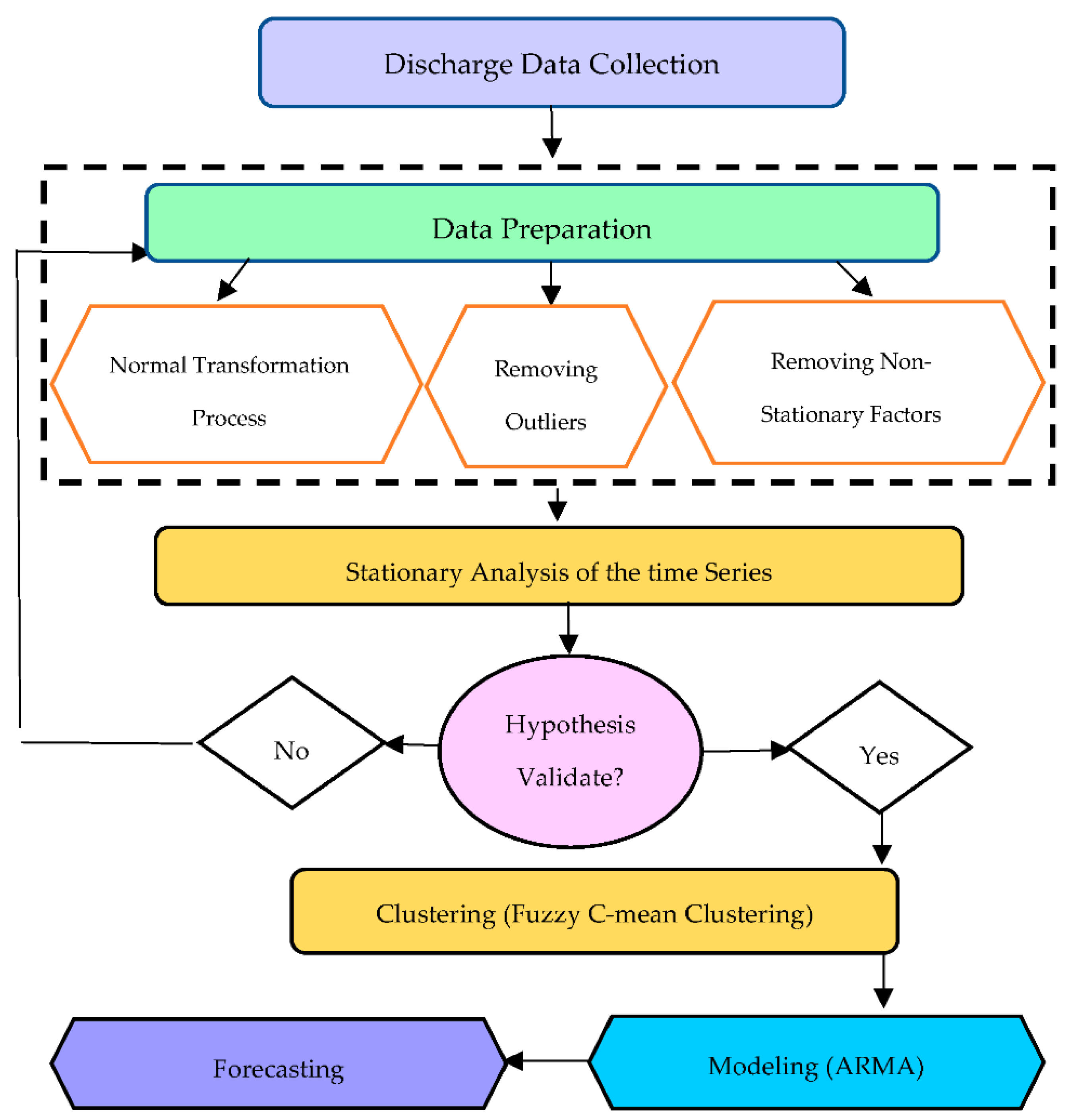
The flow chart of the methods used in this article is shown in Figure 3. As we are going to model the daily hydrological time series, which are usually periodic, we have to deal with them periodically and find the periods with similar behavior to put them into the same group. Therefore, as one of the data mining methods, the first Fuzzy cluster (see Section 2.3.1) has been applied to the time series to achieve the aim mentioned above. Then ARMA model (see Section 2.3.2) is utilized to find the best-fitted model for each cluster. Finally, a ten-point forecast was made for each cluster.

2.3.1. Augmented Dickey Fuller Test (ADF)

Trend and seasonality are the most important factors that cause time series to be nonstationary. Identifying the effects of these factors can be done by using stationary tests [35]. There are many different methods to test whether a time series is stationary or not. Among them, an ADF test has been used and is acknowledged to test the stationary of stream flow and hydrological time series in many studies [36,37,38,39,40]. The ADF test was introduced by Dickey and Fuller in 1979 [41]. Then, in 1984, Said and Dickey improved it [42]. The main equation of ADF is as follows:

$$\mathrm{\Delta }{\mathrm{Y}}_{\mathrm{t}}=\mathsf{\alpha }+\mathsf{\beta }\mathrm{t}+{\mathsf{\gamma }\mathrm{Y}}_{\mathrm{t}-1}+{{\displaystyle \sum }}_{\mathrm{j}=1}^{\mathrm{p}}({\mathsf{\delta }}_{\mathrm{j}}\mathrm{\Delta }{\mathrm{Y}}_{\mathrm{t}-\mathrm{j}})+{\mathsf{\epsilon }}_{\mathrm{t}}$$

(1)

where $\mathrm{t}$ is the time index, $\mathsf{\alpha }$ is an intercept constant called drift, $\mathsf{\beta }$ is the coefficient on a time trend, $\mathsf{\gamma }$ is a coefficient presenting process root, $\mathrm{p}$ is the lag order of the first differences autoregressive process, and ${\mathrm{e}}_{\mathrm{t}}$ is an independent, identically distributed residual term.

2.3.2. Fuzzy C-Mean Cluster (FCM)

Based on a Fuzzy cluster, every object in a dataset can join more than one cluster. One of the most widely used kinds of Fuzzy clusters is FCM. Allocating a degree of membership for every member in every cluster is the technique that FCM uses for decreasing the uncertainly in recognizing the members. [43,44]. It calculates the distance of every object from the cluster center and specifies the class of every object by optimizing the target function based on the minimum square error. It is proposed that ${\mathrm{X}}_{\mathrm{t}}=\left\{{\mathrm{X}}_1,{\mathrm{X}}_2,\dots ,{\mathrm{X}}_{\mathrm{N}}\right\}$. The FCM cluster partitions ${\mathrm{X}}_{\mathrm{t}}$ into a collection of C clusters, $\mathrm{C}=\left\{{\mathrm{c}}_1,{\mathrm{c}}_2, \dots ,{\mathrm{c}}_{\mathrm{c}}\right\}$, by an iterative minimization with respect to defined criteria [45]. The process of its objective function is defined below:

$${\mathrm{J}}_{\mathrm{CM}}={{\displaystyle \sum }}_{\mathrm{j}=1}^{\mathrm{c}}{{\displaystyle \sum }}_{{\mathrm{x}}_{\mathrm{i}\in {\mathrm{c}}_{\mathrm{j}}}}\Vert {\mathrm{x}}_{\mathrm{i}}-{\mathsf{\theta }}_{\mathrm{j}}\Vert {}^2$$

(2)

where ${\mathrm{C}}_{\mathrm{j}}$ is the $\mathrm{j}$th cluster and ${\mathsf{\theta }}_{\mathrm{j}}$ is its centroid and ‖ ‖ is the Euclidean distance. Every $\mathrm{X}$ will be placed in the nearest cluster in each repeat. Then, cluster centroids will be updated as follows:

$${\mathsf{\theta }}_{\mathrm{j}}=\frac{1}{{\mathrm{N}}_{\mathrm{j}}}{\displaystyle {{\displaystyle \sum }}_{{\mathrm{x}}_{\mathrm{i}}\in {\mathrm{C}}_{\mathrm{j}}}}{\mathrm{X}}_{\mathrm{i}}$$

(3)

where ${\mathrm{N}}_{\mathrm{j}}$ is the object number in cluster $\mathrm{j}$ and is subjected to ${\displaystyle \sum }_{\mathrm{j}=1}^{\mathrm{C}}{\mathrm{N}}_{\mathrm{j}}={\mathrm{N}}_0$.

2.3.3. ARIMA Model

An autoregressive integrated moving average, or ARIMA, is a statistical analysis model that uses time series data to either better understand the data set or to predict future trends and enables the description and analysis of time series. An ARIMA model includes two stationary models, AR (autoregressive) and MA (moving average). To explain it more clearly, AR shows how a variable in a time series is connected to its lagged value, and MA is the linear mixture between an object and errors of previous objects. “I” is the value of difference between an observation and previous ones to reach the stationary [46]. Therefore, if a time series is stationary, the ARIMA model will change to the ARMA model. In this case, d will be zero. The general mathematic forms of ARIMA (p, d, q) and ARMA (p, q) are defined as follows [47]:

$$\mathrm{ARIMA}:{ \mathsf{\phi }}_{\mathrm{P}}\left(\mathrm{B}\right){\nabla }^{\mathrm{d}}{\mathrm{x}}_{\mathrm{t}}={\mathsf{\theta }}_{\mathrm{q}}\left(\mathrm{B}\right){\mathsf{\epsilon }}_{\mathrm{t}}$$

(4)

$$\mathrm{ARMA}:{ \mathsf{\phi }}_{\mathrm{P}}\left(\mathrm{B}\right){\mathrm{x}}_{\mathrm{t}}={\mathsf{\theta }}_{\mathrm{q}}\left(\mathrm{B}\right){\mathsf{\epsilon }}_{\mathrm{t}}$$

(5)

where B is the backward operator $\left({\mathsf{\beta }\mathrm{x}}_{\mathrm{t}}={\mathrm{x}}_{\mathrm{t}-1}\right)$ and $\nabla {\mathrm{x}}_{\mathrm{t}}={\mathrm{x}}_{\mathrm{t}}-{\mathrm{x}}_{\mathrm{t}-1}$ is a stationary process. The AR component is $\mathsf{\phi }\left(\mathrm{B}\right)$ with p order, the MA component is $\mathsf{\theta }\left(\mathrm{B}\right)$ with q order, and d is a differencing parameter which is used to ensure data stability. Parameters of the ARIMA and ARMA models, p and q, have been estimated by an autocorrelation function graph (ACF) and partial autocorrelation correlogram (PACF).

2.3.4. Performance Metric

Root mean square error (RMSE) is utilized for evaluating the modeling outcome as a performance metric. The general form of RMSE is as follows:

$$\mathrm{RMSE}=\sqrt{\frac{1}{\mathrm{M}}{{\displaystyle \sum }}_{\mathrm{i}=1}^{\mathrm{M}}{\left({\mathrm{P}}_{\mathrm{i}}-{\mathrm{O}}_{\mathrm{i}}\right)}^2}$$

(6)

where M is the number of observations, ${\mathrm{P}}_{\mathrm{i}}$ is the estimated value, and ${\mathrm{O}}_{\mathrm{i}}$ is the actual observation. The lower the value, the more accurate the prediction [48].

3. Results

After preprocessing the data by normalization and removing the nonstationary factors containing trend and seasonality, they became ready for operation, and the results are divided into four parts: normalization, clustering, modeling, and forecasting.

3.1. Normalization

The purpose of the stationarity test is to answer the question of whether the mean and variance values change over time or not. Most of the time series are nonstationary due to different reasons, such as trend or periodicity. They should be stationary before modeling [49]. To fulfill this purpose, an ADF test has been used for testing stationarity. The trend should be omitted before applying the ADF test. To reach this goal, the data has been standardized by subtracting the mean from them and dividing by the standard deviation. Finally, the stationarity of the data was examined.

Table 2. Results of ADF test for daily discharge with 95% confidence.

Station	Lag	ADF Unit Root		Result
		ADF Statistic	p-Value
Biedenkopf	4	−14.42241	0	Stationary
Ehringen	13	−7.734843	0	Stationary
Günthers	10	−11.47729	0	Stationary
Hanau	6	−12.90913	0	Stationary

shows the results of the ADF test at the 95% confidence level.

3.2. Clustering

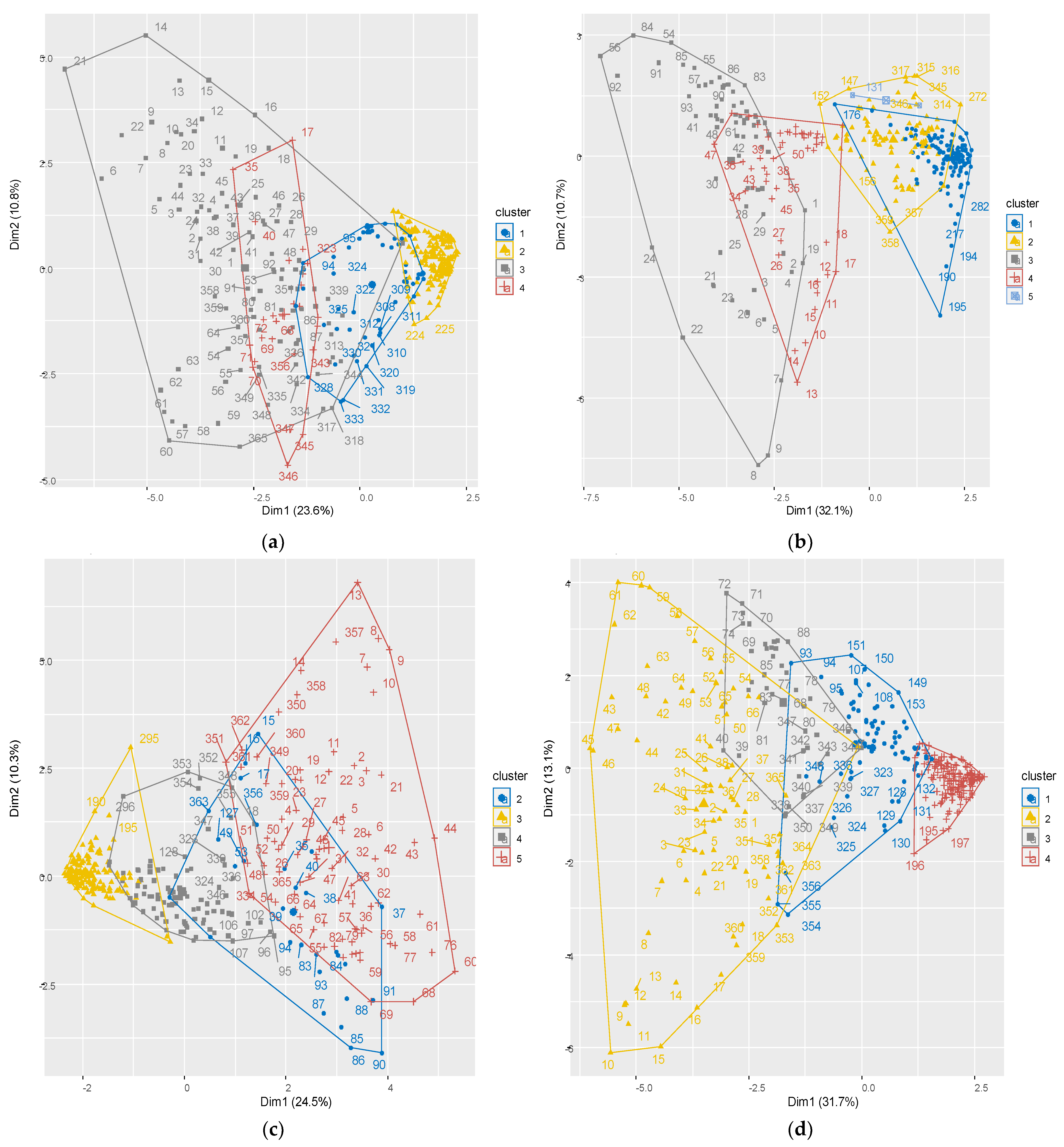
Due to the periodic behavior of hydrologic time series, their periodic classification based on days with similar statistical behavior and not based on season or month will give more realistic results. To achieve this aim, we divided the days with similar statistical behavior for each station using the Fuzzy C-means cluster method, frequently used in pattern recognition. Based on this, Biedenkopf is divided into four clusters, Ehringen five, Günthers four, and Hanau four clusters. After checking the days placed in each cluster, it was found that some days in the same cluster are not consecutive in three stations. Therefore, to place the days which are in order in the same cluster, we made some changes in the number of clusters for those stations. After applying the method described above, Biedenkopf, with the decrease of one number in the number of clusters, decreased from four clusters to three clusters, the day 1 to day 81 into cluster number two, the day 82 to day 299 into cluster number one, and day 300 to the last day into cluster number five. This reduction in the number of clusters has been made for Ehringen as well, but for this station, from five to three. Thus, the days in Ehringen are classified as day 1 till day 107 and placed into cluster number three, day 108 till day 189 into cluster number two, and the rest into cluster number one. However, there was not any change in the numbers of clusters for Günthers, and they remained divided into four, day 1 till day 90 in cluster number five, day 91 to day 151 in cluster number four, day 152 to day 295 in cluster number three and the others into cluster number one. In addition, for the last station, Hanau, the number of clusters increased from four to five, from day 1 to day 59 into cluster number two, day 60 to day 90 into cluster number three, from day 91 to day 151 into cluster number one, from day 152 to day 304 into cluster number four, and the rest in cluster number five.

Table 3. Numbers of Clusters.

Station	Clusters		No of Cluster	Days	Average (m3/s)	Standard Deviation (m3/s)	Skewness (m3/s)	Kurtosis (m3/s)
	Before Editing	After Editing
Biedenkopf	4	3	2	1–81	9.91	11.31	3.04	12.66
			1	82–299	2.63	4.14	5.86	59.38
			5	300–365	7.42	8.84	3.43	20.55
Ehringen	5	3	3	1–107	0.95	0.67	3.66	22.57
			2	108–189	0.60	0.54	12.64	265.76
			1	190–365	0.48	0.48	13.61	365.05
Günthers	4	4	5	1–90	4.46	4.67	4.21	25.73
			4	91–151	2.52	2.86	6.85	65.60
			3	152–295	1.26	1.44	9.87	161.24
			1	296–365	2.85	2.93	4.50	33.55
Hanau	4	5	2	1–59	18.19	15.74	2.73	9.97
			3	60–90	15.18	11.09	2.11	6.31
			1	91–151	8.57	6.70	2.68	9.08
			4	152–304	5.34	3.95	4.04	22.39
			5	305–365	12.02	9.90	2.24	6.91

presents the summary of clustering results for each station, and Figure 4 represents the plot of time series clustering before editing.

3.3. Modeling

Identifying the behavioral pattern of stream flow can be a powerful aid in managing hydrological issues. Applying stochastic hydrology to recognize the streamflow models is one of the most practical methods and was introduced in 1964 [35].

As a statistical powerful linear model, the autoregressive moving average (ARIMA) is strongly approved by researchers [50], which is a kind of nonstationary variation of the ARMA model. Therefore, the ARMA model is extracted for stationary time series [47].

After applying the process described above for clustering and indicating the cluster numbers for each station, the ARMA model was extracted for each group to assess. Finally, the results of the best-fitted models at a daily scale have been represented in

Table 4. Summary of ARMA model parameters.

Station	Cluster	Model	Coefficients		AIC	RMSE
			p	q
Biedenkopf	1	ARMA (2,2)	1.7309	−0.6591	2948.53	0.351
			−0.7386	−0.1691
	2	ARMA (2,2)	1.5614	−0.2682	−793.42	0.183
			−0.6116	−0.1553
	5	ARMA (1,2)	0.9088	0.3375	855.98	0.345
				0.0663
Ehringen	1	ARMA (3,1)	1.5526	−0.8009	3409.21	0.413
			−0.6217
			0.0598
	2	ARMA (1,2)	0.9713	−0.5694	2859.04	0.634
				−0.1744
	3	ARMA (2,2)	1.5592	−0.4584	871.71	0.302
			−0.5718	−0.3568
Günthers	1	ARMA (1,2)	0.8925	0.0967	952.29	0.351
				−0.1803
	3	ARMA (2,2)	1.5167	−0.6099	−0.04	0.241
			−0.5324	−0.135
	4	ARMA (1,1)	0.8952	−0.5683	2718.4	0.831
	5	ARMA (1,1)	0.8292	0.2832	861.77	0.314
Hanau	1	ARMA (1,3)	0.9226	0.1881	1092.25	0.395
				−0.2797
				−0.1445
	2	ARMA (2,1)	1.2575	0.1114	−2045.8	0.091
			−0.3416
	3	ARMA (2,0)	1.2172	0	−541.66	0.147
			−0.276
	4	ARMA (2,2)	1.6488	−0.6361	−9711.9	0.413
			−0.6589	−0.2077
	5	ARMA (1,2)	0.8849	0.3871	−73.8	0.232
				0.0541

. It can be seen that the model for the Hanau station, cluster number three, is ARMA (2,0). In this case, q = 0 means that this is the same model as AR (2). The accuracy of the models is indicated by the low value of RMSE and Akaike information criterion (AIC), shown in Table 4.

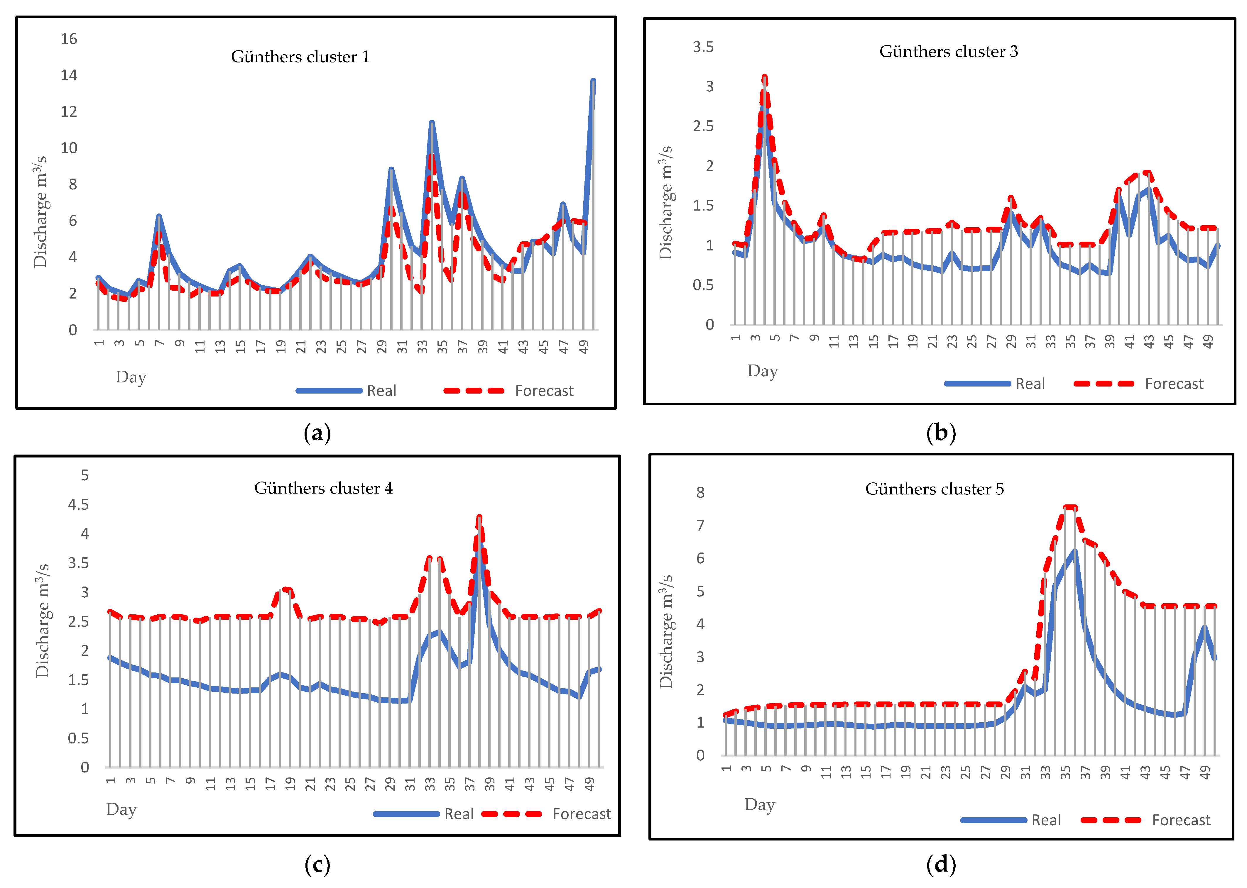
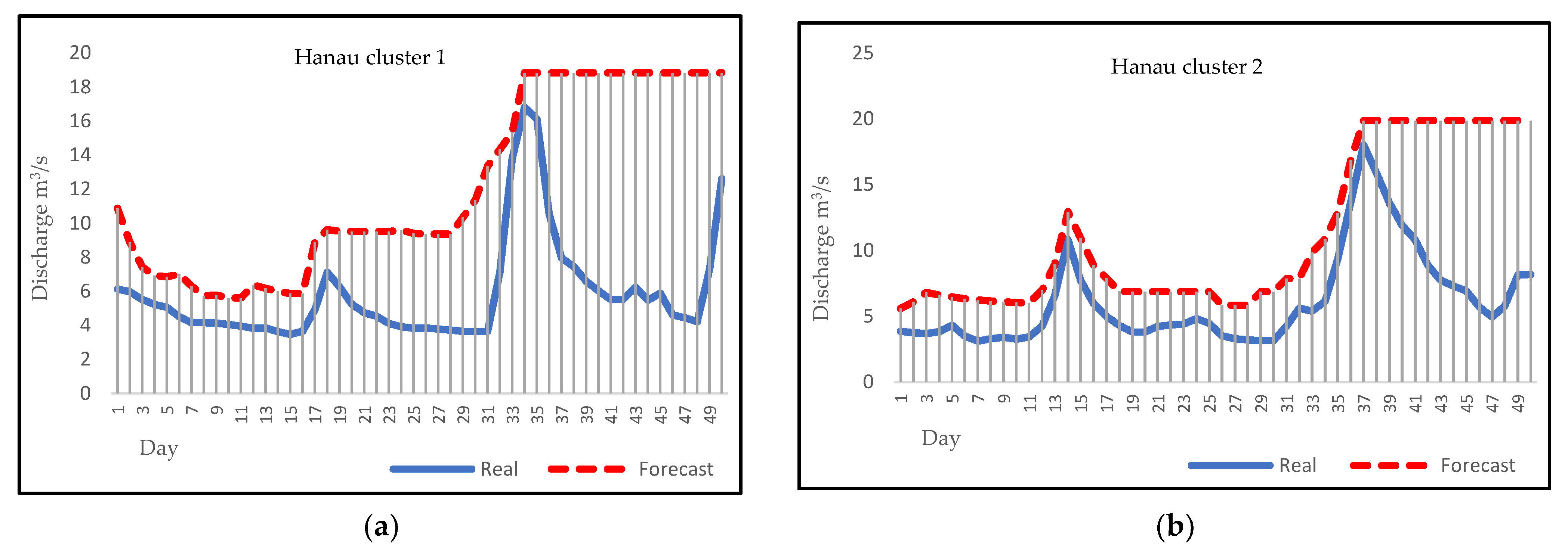
3.4. Forecasting

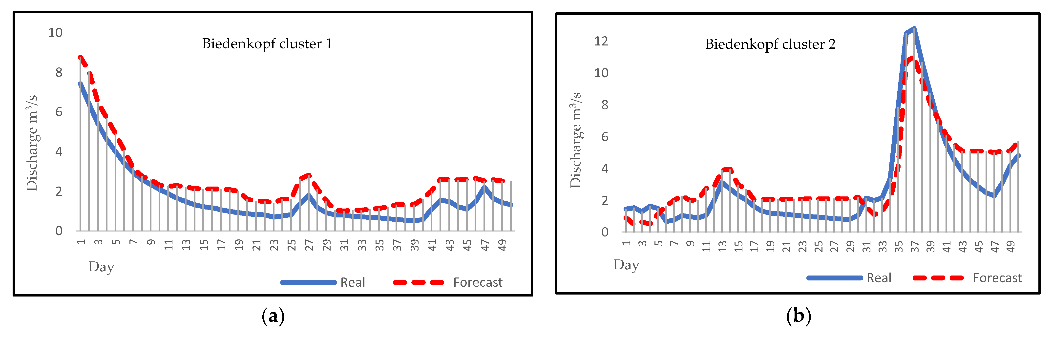
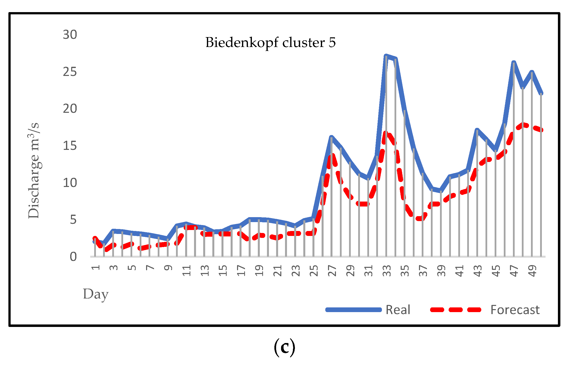
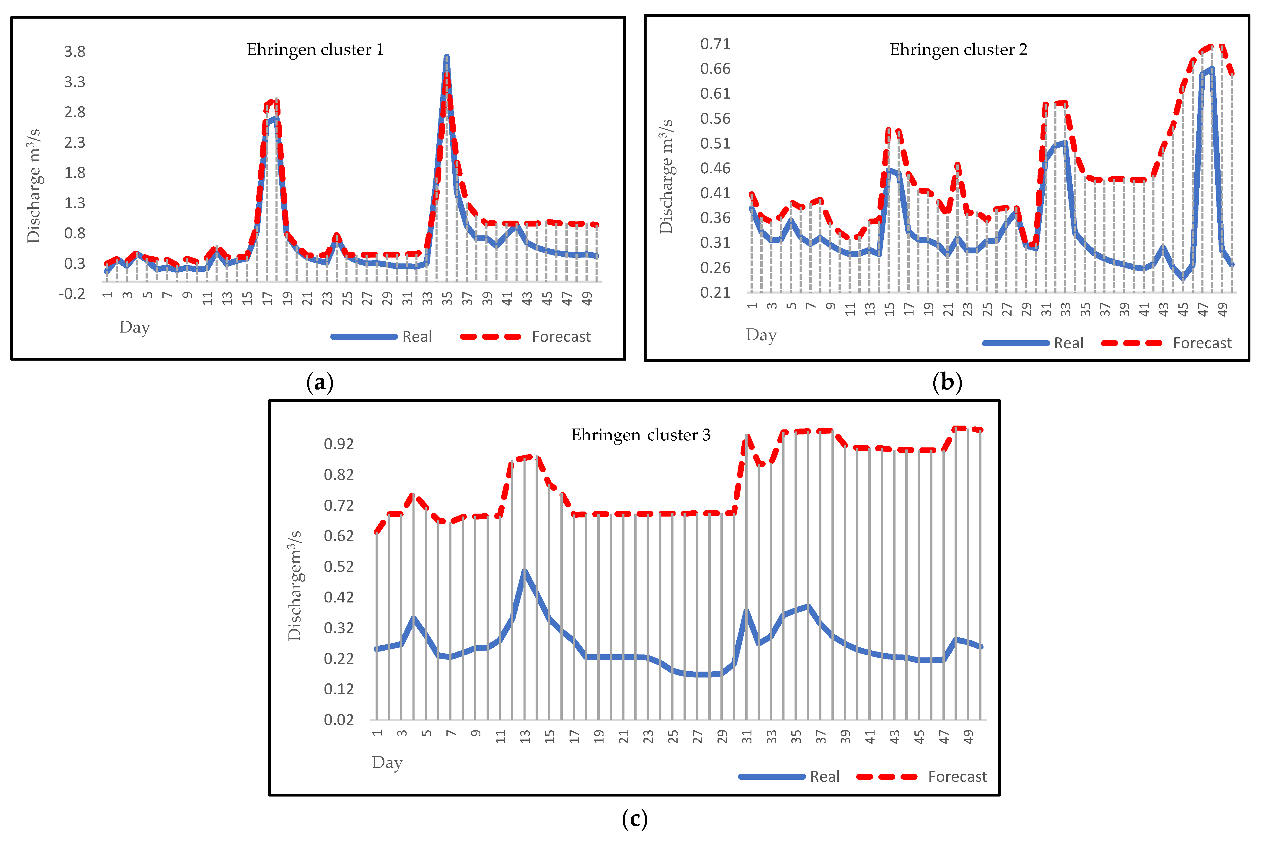
Daily discharge forecasting can be a noticeable help for flood and drought forecasting in a region, and it can reduce their damages with early warnings to communities. Figure 5, Figure 6, Figure 7 and Figure 8 represent the visual comparison of predicted values with true values of Biedenkopf, Ehringen, Günthers, and Hanau stations, respectively. A total of 50 days of forecasting, for the first 50 days of each cluster, has been done for all clusters except Hanau cluster 3, because there are 31 days in this cluster.

4. Discussion

Daily streamflow and time series show more fluctuations than series, which are classified based on a monthly, seasonal, or annual scale. Decomposing the daily series into their components, such as trend, cyclic, seasonal, or irregularity, is almost impossible compared to monthly or seasonal series. Hydrological daily series clustering based on the Fuzzy C-means (FCM) method divides every series into subseries with similar behavior. Therefore, there will be several series with different lengths instead of one series. As a result, all daily streamflow time series were observed to exhibit periodicity. Figure 4 presents the cluster plots of these four selected stations graphically, tabulated in Table 3. As shown in Figure 4, the continuous lines specify the limitation area for each cluster, and every day is placed in a cluster exclusively. According to the FCM method, every day will be set in the cluster with the smallest distance from the average of that cluster. This way, the days with similar statistical behavior have been placed in one cluster.

Considering previous research, daily streamflow time series have more powerful long-memory and nonlinearity properties than monthly or seasonal time series [35,51]. By decomposing the main daily streamflow time series into several smaller subseries using FCM, the behavior of this smaller subseries will tend to be linear. If a time series follows the linear process, modeling the time series by linear models, such as the Box–Jenkins model, can provide reliable and accurate results [52,53,54]. We evaluated the performance of the ARMA model as a linear model in forecasting the daily water discharge of each cluster. All of the collected data, from January 2000 to December 2017, was used to fit the best model on each cluster. Table 4 represents the ARMA model details for each cluster. The criterion for evaluating the fitted models was the low value of RMSE and the Akaike coefficient, which are given in the last two columns of Table 4.

After applying the algorithms described above to four different sampling stations, forecasting results were evaluated and compared by dividing the data into two parts for training and testing. The fitted model was applied to the data from January 2000 to December 2016 for the 2017 forecast. Then, forecasting plots for 2017 were compared with the historical plots to evaluate the model. Figure 5, Figure 6, Figure 7 and Figure 8 present the visual comparison between each cluster’s forecasting and observation plots. The continuous line indicates the observation plot, and the dashed line indicates the forecasting plot, which is the output of our models. Based on our results, forecasting graphs for all clusters have a clearly evident flow rate changes trend and optimal points. This result corresponds to the ARMA model and, compared to other studies’ results, confirms the accurate and reliable results of the ARMA model as a linear model; these results also prove this issue. [55,56,57]. On the other hand, the forecast charts show that the ARMA model has performed well for forecasting less than thirty days. This result is consistent with the results of previous research. Based on previous research, ARMA models are known as short-term models and will be more beneficial for short-term forecasting [58,59,60].

5. Conclusions and Outlook

This paper underlines the importance of Fuzzy clustering on the periodic autoregressive ARMA model for stream flow forecasting. As a result of climatic influences, hydrological processes behave in a periodic and stochastic manner. In order to make accurate predictions, it is crucial to develop the models based on their periodicity and stochastic nature. Streamflow forecasting is also a primary subject since it is an important component of the hydrological cycle. Fuzzy C-means clusters were used to find the periodicity in the daily discharge time series, and autoregressive moving average, ARMA, was employed to model each cluster. Using a statistical method, dividing the daily streamflow time series into smaller groups based on their similar statistical behavior was done. Our analysis was based on the daily discharge data from four different river stations in the German state of Hesse.

Regarding the results obtained in this study that focuses on four stations in Hesse, decreasing the length of periodic time series and using linear models is highly recommended. By clustering the days of the year and modeling every cluster separately, linear time series will exist, and forecasting different days of the year based on the cluster formed will be possible. This method of segmentation and modeling, described here, can also be used for short-term prediction at other hydrological stations. As a disadvantage of this method, converting a time series into several subseries and modeling each cluster separately is time-consuming. For future work, using different statistical methods—such as decision trees, wavelets, or machine learning—to decompose the original series into subseries of days and comparing the modeling results is recommended.

References

- Bai, Y.; Wang, P.; Li, C.; Xie, J.; Wang, Y. A multi-scale relevance vector regression approach for daily urban water demand forecasting. J. Hydrol. 2014, 517, 236–245. [Google Scholar] [CrossRef]
- Abbaspour, K.C.; Faramarzi, M.; SeyedGhasemi, S.; Yang, H. Assessing the impact of climate change on water resources in Iran. Water Resour. Res. 2009, 45, W10434. [Google Scholar] [CrossRef] [Green Version]
- Tekieh, M.H.; Raahemi, B. Importance of data mining in healthcare: A survey. In Proceedings of the ACM International Conference on Advances in Social Networks Analysis and Mining, Paris, France, 25–28 August 2015. [Google Scholar]
- Lee, S.J.; Siau, K. A review of data mining techniques. Ind. Manag. Data Syst. 2001, 101, 41–46. [Google Scholar] [CrossRef] [Green Version]
- Weiss, S.M.; Indurkhya, N. Predictive Data Mining: A Practical Guide, 1st ed.; Morgan Kaufmann Publishers, Inc.: San Francisco, CA, USA, 1998; pp. 1–2. [Google Scholar]
- Fayyad, U.; Piatetsky-Shapiro, G.; Smyth, P. From Data Mining to knowledge Discovery in Databases. Al Mag. 1996, 17, 37–54. [Google Scholar] [CrossRef]
- Coenen, F. Data mining: Past, Present and Future. Knowl. Eng. Rev. 2011, 26, 25–29. [Google Scholar] [CrossRef]
- Liu, J.; Zhou, S. Application Research of Data Mining Technology in Personal Privacy Protection and Material Data Analysis. Integr. Ferroelectr. 2021, 216, 29–42. [Google Scholar] [CrossRef]
- Ekasingh, B.; Ngamsomsuke, K.; Letcher, R.A.; Spate, J. A data mining approach to simulating farmers’ crop choices for integrated water resources management. J. Environ. Manag. 2005, 77, 315–325. [Google Scholar] [CrossRef]
- Habibipour, A.; Mahjoubi, J.; Dastourani, M.T. Investigation of ability of some data mining methods in studies related to water resources. In Proceedings of the First Regional Water Resources Development Conference, Azad University, Abar Kooh, Iran, 19 May 2011. [Google Scholar]
- Wei, W.; Watkins, D.W., Jr. Data Mining Methods for Hydro Climatic Forecasting. Adv. Water Resour. 2011, 34, 1390–1400. [Google Scholar] [CrossRef]
- Nourani, V.; Sattari, M.T.; Molajou, A. Threshold-Based Hybrid Data Mining Method for Long-Term Maximum Precipitation Forecasting. Water Resour. Manag. 2017, 31, 2645–2658. [Google Scholar] [CrossRef]
- Berkhin, P. Grouping Multidimensional Data, 1st ed.; Springer: Berlin/Heidelberg, Germany, 2006; pp. 25–71. [Google Scholar]
- Luczak, A.; Kalinowski, S. Fuzzy Clustering Methods to Identify the Epidemiological Situation and Its Changes in European Countries during COVID-19. Entropy 2021, 24, 14. [Google Scholar] [CrossRef]
- Zhang, X.; Zhang, C.; Tang, W.J.; Wie, Z.W. Medical Image Segmentation Using Improved FCM. Sci. China Inf. Sci. 2012, 55, 1052–1061. [Google Scholar] [CrossRef] [Green Version]
- Aydogdu, M.; Firat, M. Estimation of Failure Rate in Water Distribution Network Using Fuzzy Clustering and LS-SVM Methods. Water Resour. Manag. 2014, 29, 1575–1590. [Google Scholar] [CrossRef]
- Mosavi, A.; Golshan, M.; Choubin, B.; Ziegler, A.D.; Sigaroodi, S.K.; Zhang, F.; Dineva, A.A. Fuzzy clustering and distributed model for streamflow estimation in ungauged watersheds. Sci. Rep. 2021, 11, 8243. [Google Scholar] [CrossRef] [PubMed]
- Latt, Z.Z.; Wittenberg, H.; Urban, B. Clustering Hydrological Homogeneous Regions and Neural Network Based Index Flood Estimation for Ungauged Catchments: An Example of the Chindwin River in Myanmar. Water Resour. Manag. 2015, 29, 913–928. [Google Scholar] [CrossRef]
- Maruyama, T.; Kawachi, T.; Singh, V.P. Entropy-based assessment and clustering of potential water resources availability. J. Hydrol. 2005, 309, 104–113. [Google Scholar] [CrossRef]
- Ebrahimi Varzane, A.; Zarei, H.; Tishehzan, P.; Akhondali, A.M. Evaluation of Groundwater-Surface Water Interaction by Using Cluster Analysis (Case Study: Western Part of Dezful-Andimeshk Plain). Iran-Water Resour. Res. 2019, 15, 246–257. [Google Scholar]
- Kottegoda, N.T. Stochastic Water Resources Technology, 1st ed.; The Macmillan Press Ltd.: London, UK, 1980; pp. 20–21. [Google Scholar]
- Jones, R.H.; Brelsford, W.M. Time Series with Periodic Structure. Biometrika 1967, 54, 403–408. [Google Scholar] [CrossRef]
- Pagano, M. On Periodic and Multiple Autoregression. Inst. Math. Stat. 1978, 6, 1310–1317. Available online: https://www.jstor.org/stable/2958718 (accessed on 20 October 2022). [CrossRef]
- Troutman, B.M. Some Results in Periodic Autoregression. Biometrika 1979, 66, 219–228. [Google Scholar] [CrossRef]
- Ula, T.A. Periodic covariance stationarity of multivariate periodic autoregressive moving average processes. Water Resour. Manag. 1990, 26, 855–861. [Google Scholar] [CrossRef]
- Ula, T.A. Forecasting of Multivariate Periodic Autoregressive Moving-Average Process. J. Time Ser. Anal. 1993, 14, 645–657. [Google Scholar] [CrossRef]
- Puech, T.; Boussard, M.; D’Amato, A.; Millerand, G. A Fully Automated Periodicity Detection in Time Series. In Proceedings of the International Workshop on Advanced Analysis and Learning on Temporal Data, Cham, Germany, 23 January 2020. [Google Scholar]
- Brittanica. Available online: https://www.britannica.com/place/Hessen (accessed on 20 October 2022).
- Deutscher Wetterdienst (German Weather Service). DWD (2022): Nationaler Klimareport (National Climate Report), 6th ed.; Deutscher Wetterdienst (German Weather Service): Offenbach, Germany, 2022; 53p, ISBN 978-3-88148-536-4. [Google Scholar]
- DGJ (2017): Deutsche Gewässerkundliche Jahrbücher des Bundes und der Länder (German Hydrographic Yearbook), with Ehringen/Erpe ID 44480552 (Wesergebiet), Hanau/Kinzig ID 24784259 (Rheingebiet, Teil II, Main), Biedenkopf/Lahn ID 25810558 (Rheingebiet, Teil III), Günthers/Ulster ID 41450056 (Wesergebiet). Available online: https://www.lfu.bayern.de/wasser/wasserstand_abfluss/dgj/index.htm#:~:text=Das%20Deutsche%20Gew%C3%A4sserkundliche%20Jahrbuch%20(DGJ,und%20K%C3%BCstengebiete%20in%2010%20Teilb%C3%A4nden.&text=werden%20vom%20Bayerischen%20Landesamt%20f%C3%BCr,hydrologische%20Kenngr%C3%B6%C3%9Fen%20ausgew%C3%A4hlter%20Messstellen%20ver%C3%B6ffentlicht (accessed on 22 October 2022).
- RP Kassel (2013): Hochwasserrisikomanagementplan für das Hessische Einzugsgebiet der Diemel und Weser; Regierungspräsidium (Regional Commission): Kassel, Germany, 2013; 171p.
- Kakouei, K.; Domisch, S.; Kiesel, J.; Kail, J.; Jähnig, S.C. Climate model variability leads to uncertain predictions of the future abundance of stream macroinvertebrates. Sci. Rep. 2020, 10, 2520. [Google Scholar] [CrossRef] [PubMed] [Green Version]
- Herrig, I.M.; Böer, S.I.; Brennholt, N.; Manz, W. Development of multiple linear regression models as predictive tools for fecal indicator concentrations in a stretch of the lower Lahn River, Germany. Water Res. 2015, 85, 148–157. [Google Scholar] [CrossRef] [PubMed]
- Trabert, A.; Opp, C. Long-term trends in flood discharges of the Ulster and Upper Fulda (Germany): A statistical review. Environ. Earth Sci. 2016, 75, 1363. [Google Scholar] [CrossRef]
- Khazaiee, M.; Khalili, K.; Behmanesh, J. Investigating the relationship between physical characteristics of watersheds and nonlinearity of daily streamflow processes. Int. J. Water 2018, 12, 141–157. [Google Scholar] [CrossRef]
- Wang, W.; Wriggling, J.K.; Van Gelder, P.H.A.J.M.; Ma, J. Testing for nonlinearity of streamflow process at different time scale. J. Hudrol. 2006, 322, 247–268. [Google Scholar] [CrossRef]
- Khalili, K. Comparison pf geostatistical methods for interpolation ground water level (Case Study: Lake Urmia basin). J. Appl. Environ. Biol. Sci. 2014, 4, 15–23. [Google Scholar]
- Jarvis, D.; Stoeckl, N.; Chaiechi, T. Applying econometric Techniques to hydrological problems in a large basin: Quantifying the rainfall-discharge relationship in the Burdekin, Queensland, Australia. J. Hydrol. 2013, 496, 107–121. [Google Scholar] [CrossRef]
- Khalili, K.; Nazeri Tahrudi, M.; Khanmohammadi, N. Trend Analysis of precipitation in recent two decades over Iran. J. Appl. Environ. Biol. Sci. 2014, 4, 5–10. [Google Scholar]
- Khalili, K.; Nazeri Tahrudi, M.; Abbaszadeh Afshar, M.; Nazeri Tahroudi, Z. Modeling monthly mean air temperature using SAMS2007 (case study: Urmia synoptic station). J. Middle East Appl. Sci. Technol. 2014, 15, 578–583. [Google Scholar]
- Dickey, D.A.; Fuller, W.A. Distribution of the estimators for autoregressive time series with a unit root. J. Am. Stat. Assoc. 1979, 74, 423–431. [Google Scholar] [CrossRef]
- Said, S.E.; Dickey, D. Testing for unit roots in autoregressive moving average models with unknown order. Biometrica 1984, 71, 599–607. [Google Scholar] [CrossRef]
- Patil, S.D.; Steiglitz, M. Comparing Spatila and Temporal Transferability of Hydrological Model Parameters. J. Hydrol. 2015, 525, 409–417. [Google Scholar] [CrossRef] [Green Version]
- Choubin, B.; Solaimani, K.; Habibnejad Roshan, M.; Malekian, A. Watershed Classification by remote sensing indices: A Fuzzy C-mean Clustering Approach. J. Mt. Sci. 2017, 14, 2053–2063. [Google Scholar] [CrossRef]
- Li, Q.; Wu, X.; Zheng, J.; Wu, B.; Jian, H.; Sun, C.; Tang, Y. Determination of Pork Meat Storage Time Using Near-Infrared Spectroscopy Combined with Fuzzy Clustering Algorithms. Foods 2022, 11, 2101. [Google Scholar] [CrossRef]
- Atashi, V.; Taheri Gorji, H.; Shahabi, S.M.; Kardan, R.; Howe Lim, Y. Water Level Forecasting Using Deep Learning Time-Series Analysis: A Case Study of Red River of the North. Water 2022, 14, 1971. [Google Scholar] [CrossRef]
- Hadizadeh, R.; Eslamian, S. Hand Book of Drought and Water Scarcity, 1st ed.; CRC Press: Boka Raton, FL, USA, 2017; pp. 569–588. [Google Scholar]
- Attar, N.F.; Khalili, K.; Behmanesh, J.; Khanmohammadi, N. On the reliability of soft computing methods in the estimation of dew point temperature: The case of arid regions of Iran. Comput. Electron. Agric. 2018, 153, 334–346. [Google Scholar] [CrossRef]
- Khalili, K.; Ahmadi, F.; Dinpashoh, Y.; Behmanesh, J. Linear and Non-linear Behavior Analysis of Hydrological Time Series (Case study: Western Rivers of Lake Urmia). Iran. Water Resour. Res. 2014, 10, 12–20. [Google Scholar]
- Ho, S.L.; Xie, M.; Goh, T.N. A Comparative Study of Neural Network and Box-Jenkins ARIMA Modeling in Time Series Prediction. Comput. Ind. Eng. 2002, 42, 371–375. [Google Scholar] [CrossRef]
- Hadizade, R.; Eslamian, S.; Chinipardaz, R. Investigation of long memory properties in stream flow time series in Gamasiab River, Iran. Int. J. Hydrol. Sci. Technol. 2013, 3, 319–350. [Google Scholar] [CrossRef]
- Ghimire, B.N. Application of ARIMA model for River Discharge Analysis. Nepal Phys. Soc. 2017, 4, 27–32. [Google Scholar] [CrossRef] [Green Version]
- Yürekli, K.; Kurunç, A.; Öztürk, F. Testing the residuals of an ARIMA model on the Cekerek Stream Watershed in Turkey. Turk. J. Eng. Environ. Sci. 2005, 29, 61–74. [Google Scholar]
- Mancini, S.; Francavilla, A.B.; Longobardi, A.; Viccione, G.; Guarnaccia, C. Predicting Daily Water Tank Level Fluctuations by Using ARIMA Model, A Case Study. In Proceedings of the 5th International Conference on Applies Physics, Simulation and Computing (APSAC 2021), Salerno, Italy, 3–5 September 2021. [Google Scholar]
- Kumar, R.; Kumar, P.; Kumar, Y. Multi-Step Time Series Analysis and Forecasting Strategy Using ARIMA and Evolutionary Algorithms. Int. J. Inf. Technol. 2022, 14, 359–373. [Google Scholar] [CrossRef]
- Gui, H.; Wu, Z.; Zhang, C. Comparative Study of Different Types of Hydrological Models Applied to Hydrological Simulation. Clean Soli Air Water 2021, 49, 2000381. [Google Scholar] [CrossRef]
- Al Sayah, M.J.; Abdallah, C.; Khouri, M.; Nedjai, R.; Darwich, T. A Framework for Climate Change Assessment in Mediterranean Data-Sparse Watershed Using Remote Sensing and ARIMA Modeling. Theor. Appl. Climatol. 2021, 143, 639–658. [Google Scholar] [CrossRef]
- Ren, H.; Cromwell, E.; Chen, X. Technical Note: Using Long Short-Term Memory Models to Fill Data Gaps in Hydrological Monitoring Networks. Hydrol. Earth Syst. Sci. 2022, 26, 1727–1743. [Google Scholar] [CrossRef]
- Mehdi, H.; Pooranian, Z.; Vinueza Naranjo, P.G. Cloud Traffic Prediction Based on Fuzzy ARIMA Model with Low Dependence on Historical Data. Emerg. Telecommun. Technol. 2019, 33, e3731. [Google Scholar] [CrossRef]
- Yu, Z.; Jiang, Z.; Lei, G.; Liu, F. ARIMA Modeling and Forecasting of Water Level in the Middle Reach of the Yangtze River. In Proceedings of the 4th International Conference on Transportation Information and Safety (ICTIS), Banff, AB, Canada, 8–10 August 2017. [Google Scholar]
Figure 1.
The location of the selected stations (Ehringen, Biedenkopf, Günthers, and Hanau) on the selected rivers (Erpe, Kinzig, Lahn, and Ulster) in Hesse. Note: Source of DEM [https://www.bkg.bund.de/EN/Home/home.html (accessed on 20 October 2022)].
Figure 2.
(a) Daily discharge of Biedenkopf; (b) daily discharge of Ehringen; (c) daily discharge of Günthers; (d) daily discharge of Hanau; time scale refers to the period from 2000 to 2017.
Figure 3.
Flow chart showing the used procedure from preparing data to achieving results.
Figure 4.
(a) Cluster plot for Biedenkopf; (b) cluster plot for Ehringen; (c) cluster plot for Günthers; (d) cluster plot for Hanau.
Figure 5.
(a) Forecasting plot for Biedenkopf cluster 1; (b) forecasting plot for Biedenkopf cluster 2; (c) forecasting plot for Biedenkopf cluster 5.
Figure 6.
(a) Forecasting plot for Ehringen cluster 1; (b) forecasting plot for Ehringen cluster 2; (c) forecasting plot for Ehringen cluster 3.
Figure 7.
(a) Forecasting plot for Günthers cluster 1; (b) forecasting plot for Günthers cluster 3; (c) forecasting plot for Günthers cluster 4; (d) forecasting plot for Günthers cluster 5.
Figure 8.
(a) Forecasting plot for Hanau cluster 1; (b) forecasting plot for Hanau cluster 2; (c) forecasting plot for Hanau cluster 3; (d) forecasting plot for Hanau cluster 4, (e) forecasting plot for Hanau cluster 5.