Calibration and Validation of the FAO AquaCrop Water Productivity Model for Perennial Ryegrass (Lolium perenne L.)

Abstract

Crop models that can accurately estimate yield and final biomass have been used for major herbaceous crops and to a lesser extent in forage systems. The AquaCrop version 7.0 contains new modules that have been introduced to simulate the growth and production of perennial herbaceous forage crops. Simulated forage yields as a function of water consumption provide valuable information that allows farmers to make decisions for adapting to both climate variability and change. The study aimed to calibrate and validate the AquaCrop model for perennial ryegrass (Lolium perenne L.) in the high tropics of Colombia (South America). The experiments were conducted during two consecutive seasons, in which perennial ryegrass meadows were subjected to two irrigation regimes: full irrigation and no irrigation. The model was evaluated using precision, accuracy, and simulation error indices. The overall performance of AquaCrop in simulating canopy cover, biomass and soil water content showed a good match between measured and simulated data. The calibration results indicated an acceptable measurement of simulated canopy cover (CC) (R² = 0.95, d-index = 0.41, RMSE = 9.4%, NRMSE = 12.2%, and FE = −21.72). The model satisfactorily simulated cumulative dry mass (R² = 0.95, d-index = 0.98, RMSE = 2. 63 t ha⁻¹, NRMSE = 11.8%, and FE = 0.94). Though the biomass values obtained in the end-of-season cuts were underestimated by the model, soil water content was simulated with reasonable accuracy (R² = 0.82, d-index = 0.84, RMSE = 6.10 mm, NRMSE = 4.80%, and FE = 0.32). During validation, CC simulations were good, except under water deficit conditions, where model performance was poor (R² = 0.42, d-index = 0.01, RMSE = 40.60%, NRMSE = 40.90%, and FE = −25.71); biomass and soil water content simulations were reasonably good. The above results confirmed AquaCrop’s (v 7.0) suitability for simulating responses to water for perennial ryegrass. A single crop file was developed for managing a full season and can be confidently applied to direct future research to improve the understanding of the necessary processes and interactions for the development of perennial herbaceous forage crops.

1. Introduction

Forage planting has expanded in recent years worldwide to ensure meat and milk production. Tropical pastures consisting of grasses and legumes represent the most economical source of nutrients for livestock [1]. Ryegrass (Lolium perenne L.) is a plant species widely used in intensively managed pasture-based ruminant husbandry systems due to its ease of establishment, high digestibility, and balanced seasonal dry matter production [2]. Lolium perenne is a caespitose plant up to 80 cm in height, which produces a variable amount of tillers throughout its life. Its leaves are glabrous and have lamellae that are between 20 to 30 cm long and up to 6 mm wide. The prefoliation is conduplicate or folded. Ryegrass is a hardy and very tough species; it resprouts quickly and has a good robust rooting system, which makes it less susceptible to trampling and useful for early establishment of short- and long-term pastures. However, ryegrass crop establishment is severely affected by low water availability as well as soil nutrient deficiency [3,4].

Cattle production in Colombia in the high tropics (>2000 m.a.s.l) is characterized by the use of fodder such as ryegrass (Lolium perenne L.) as the basis of their diet; these areas contribute 32% of the national production of milk and meat. In Colombia, milk production accounts for 12% of agricultural GDP and generates 20% of agricultural employment; 17% of agricultural units produce milk [5]. Nevertheless, productivity is low and not comparable to that of the main milk and meat producing countries in the world; water availability and soil conservation are essential elements to take advantage of the forage potential of Colombia’s high tropics and improve productivity.

There is increasing uncertainty regarding water availability for agriculture. Agriculture uses up to 70% of global freshwater withdrawals, making it the largest consumer of water. The response of grasslands to drought depends on the duration, intensity, and timing of the drought, as well as the frequency of rainfall [6]. It also depends on the interactions between different factors, including diversity of the plant community, soil properties, climatic conditions, and land management [7]. Grassland productivity is expected to be affected by climate change [8,9]; however, there is great uncertainty regarding the biomass productivity of grasslands in tropical regions under changing climatic conditions. The Institute of Hydrology, Meteorology and Environmental Studies of Colombia predicted increases in the country’s average temperature of 0.9 °C, 1.6 °C, and 2.14 °C for 2040, 2070, and 2100, respectively, and a decrease in rainfall of between 10% and 40% in a third of the country (mainly in the Andean zone and the high tropics of Colombia) [10]. Farmers can adapt to climate variability by choosing different grass species or cultivars and adjusting management practices, such as irrigation application strategies and selection of planting and harvest dates.

Most of the models adapted for the cultivation of perennial ryegrass have been developed for cold temperate climatic conditions in Nordic countries. In addition, the simulations of biomass accumulation are a function of temperature and light availability, and this limits their accuracy in predicting pasture productivity in tropical and subtropical regions. The models that have so far been used to model the biomass of perennial ryegrass are BASGRA [11], LINGRA [12], and PaSIM [13]; these models were designed to simulate the dynamics of grass monocultures in Norway and Finland during successive years and under repeated defoliation. In these three models, biomass accumulation is based on the concept of radiation use efficiency, where inter-accepted solar radiation is converted to biomass. These are typically complex models and require numerous input parameters.

Some well-known models have already been adapted with satisfactory results for tropical pastures and forage: the AgPasture model [14,15], integrated in the APSIM package (‘The Agricultural Production Systems sIMulator’) simulates mixed C3 and C4 grass and legume pastures; APSIM-Growth [16] simulates the growth of tropical pastures as a function of radiation use efficiency; APSIM-Tropical Pasture [17] was used to simulate Brachiaria brizantha growth; CROPGRO-PFM [18,19,20] is a mechanistic model of the Decision Support System for Agrotechnology Transfer (DSSAT) platform, to simulate forage production and has been widely explored in Brazil.

In this context, the Food and Agriculture Organization of the United Nations (FAO) developed the AquaCrop simulation model to assist consultants, irrigation engineers, agronomists, (non-)governmental organizations, and even farm managers with the formulation and evaluation of guidelines for increasing crop water productivity with improved agronomic practices [21].

In the AquaCrop model, the biophysical processes are simplified so that the amount of data required for input and calibration remains limited, while robustness and accuracy are protected [22]. The AquaCrop model was initially developed for herbaceous food crops, although forage crops are now being considered [23,24,25]. A growing community of AquaCrop users is continuously adding new crops. Simulation models for tropical grasses can benefit forage researchers and farm managers by improving forage production systems in tropical regions as well as providing information in climate variability scenarios on yield gaps and production risk analysis.

This study aims to calibrate and validate the AquaCrop model for Perennial ryegrass (Lolium perenne L.) in the Colombian high tropics. Therefore, we use experimental field data collected in two cropping seasons to generate the parameter crop file required to run a simulation with the AquaCrop model.

2. Materials and Methods

2.1. AquaCrop Model Description

The Food and Agriculture Organization of the United Nations—FAO—developed the AquaCrop model [26]. AquaCrop uses the water productivity as a growth driver. The model requires field-level observations and provides a reasonable compromise between detailed, targeted crop yield simulation models and simplistic experimental models with considerable accuracy, robustness, and user-friendliness [23]. Model inputs include climate observations, different field data including soil profile, irrigation and farm management practices, and crop phenological growth stages in terms of their thermal time or calendar day requirements.

The AquaCrop model calculates the daily water balance by separating transpiration and evaporation. Transpiration and evaporation are correlated with the area of vegetated and unvegetated ground cover, respectively. Plant response to water stress is modelled as a function of leaf expansion, stomatal conductance, early canopy senescence, and change in harvest index. Subsequently, the model simulates the yield and biomass from daily transpiration values (Equations (1) and (2)).

$$Y=HI\times B$$

(1)

$$B=WP\times {{\displaystyle \sum }}^{ }Tr$$

(2)

where B = above ground biomass (t ha⁻¹), WP = water productivity (kg m⁻³), Tr = crop transpiration (m³ ha⁻¹), HI = harvest index, and Y = yield (t ha⁻¹).

FAO recently published the new version of AquaCrop (V. 7.0), in which new advances were introduced; the most important is the module to simulate the growth and production of perennial herbaceous forage crops, as tested with alfalfa. In addition, its procedures include describing reduction of plant population over time, the translocation of nutrients from the canopy to the root system from season to season, the growth of the canopy and forage crop management between cutting events, the programming of the cuts and the number of them within the growth cycle in the medium and long term, and the calculation of the ET₀ based on the climate information introduced in the model [27]. The new version of AquaCrop 7.0 considers the transfer of nutrients from the canopy to the root system of the crop, which usually occurs after the middle of the annual season in perennial herbaceous forage crops; this fraction can be considerable. When the following season begins, the fraction of the nutrients stored in the roots is mobilized towards the crop canopy. The model assumes that part of the nutrients is lost during the low respiration season and due to the natural reduction of the canopy or remains stored in the roots. The new module for perennial herbaceous forage crops considers several cuts during their growth and development. The users can program or generate the harvests according to their cuts within some criteria [28].

2.2. Study Site

Two field experiments were conducted in the growing seasons of 2008 to 2010 in equatorial highland zones of Colombia at the Colombian Corporation of Agricultural Research (AGROSAVIA), Tibaitatá Research Center, Colombia (4°42′ N; 74°12′ W; 2543 m a.s.l.). Long-term climate data from the Tibaitata Research Center (1954–2020) shows rainfall of approximately 657 mm per year on average, concentrated in the winter (March–July and October–November). Moreover, the average maximum temperature in January is 16.4 °C, and the minimum temperature is about 9.7 °C. The mean relative humidity is 77.9–83.8%, and the average daily reference evapotranspiration is 2.83 mm day⁻¹.

2.3. Experimental Setup and Irrigation Water Management

The fields trials were conducted during two successive growing seasons: the first (used for calibration of the AquaCrop model) spanned from 19 December 2008 until 2 February 2010. The second growing season (used for AquaCrop model validation) spanned from 10 February 2010 until 7 October 2010. The field experiments were conducted on a 36 m by 40 m plot, and the soil of the experimental site is an Andisol with a silty loam texture.

The perennial ryegrass cultivar used for the calibration and validation experiments of the AquaCrop model was Bestfor Plus, the most widely grown variety in the high tropics of Colombia. A seeding rate of 50 kg ha⁻¹ was used. A total of 6.6 kg of seeds were distributed uniformly by hand over 1440 m². After sowing, irrigation was carried out in order to ensure uniform soil moisture throughout the experimental area and to facilitate seed germination. A compound fertilizer, such as NPK (15-15-15) and magnesium sulphate, was used.

In both growing seasons, the experiment was laid out in randomized complete blocks with six irrigation regimes and eight replications. The irrigation regimes included full-irrigation (irrigation based on 100% field capacity (FC)), mild water stress (60% FC), moderate water stress (50% FC), severe water stress (40% FC), most severe water stress (20% FC) and non-irrigated (<20% FC). The irrigation regimes were applied using a linear source sprinkler irrigation system that allowed long-term evaluation of crop yield under continuous irrigation gradients, from over-irrigation to no irrigation [29,30]. The irrigation depth rate was 13.49 mm h⁻¹ lower than the basic infiltration rate of 21.6 mm h⁻¹, to avoid surface water ponding and runoff; thus, the irrigation system design was suitable for the soil type. The distribution uniformity was 86%, while the distribution uniformity of the lateral whole was 83.52%. The Christiansen uniformity coefficient was 89.59%, and the irrigation efficiency was 68.6%. The sprinklers used were the Toro Irrigation brand, model S-II, with an operating pressure of 249.76 kPa (36.25 psi). However, according to the guidelines specified by Hsiao et al. [31] for the calibration, the “full irrigation” level was used for guaranteeing that the crop was evaluated at the maximum levels of performance and was validated with the “non-irrigated” level, which presents the most adverse conditions for the development of the crop.

The irrigation treatments used for calibration and validation of the AquaCrop model were identified as follows: C1-Irrigation: full irrigation treatment in the first cropping season of ryegrass (December 2008 to February 2010); C1-Non-Irrigated: non-irrigated treatment in the first cropping season of ryegrass (December 2008 to February 2010); C2-Irrigation: full irrigation treatment in the second cropping season of ryegrass (February 2010 to October 2010); C2-Non-Irrigated: non-irrigated treatment in the second cropping season of ryegrass (February 2010 to October 2010).

Soil moisture was measured every two days at a depth ranging from 0 to 30 cm, using the thermogravimetric method and TDR equipment. The water balance was obtained to determine evapotranspiration, assuming negligible surface runoff and evaluating deep percolation, defined as the water above the FC point under the roots. Actual evapotranspiration per experimental unit was determined by obtaining K_T, Ke, and Kc using the Penman-Monteith method [32].

2.4. Phenological Data of the Ryegrass Crop (Lolium perenne L.)

Phenological data in calendar days and thermal time—growing degree days (GDD)—were obtained after field monitoring of the ryegrass crop; the main growth stages were defined, and early canopy senescence was not considered because Lolium perenne does not reach that stage. Degree days were calculated following the methodology described in the AquaCrop reference manual [21]. The AquaCrop model uses thermal time to determine green canopy cover and is crucial for crop development. Crop phenology data are shown in

Table 1. Phenological stages in calendar days and cumulative growing degree days (GDD) required from sowing to emergence and for maximum canopy cover of ryegrass (Lolium perenne L.) across two growing seasons.

Phenological Stages	Calendar Days	Growing Degree Days
Time from planting to emergence 90%	9	83.6
Stage in boot	62	550.9
Maximum effective rooting depth	64	570.9
First spikelet visible	69	616.9
Time period to flowering	83	755.0
Time from planting to max. canopy cover	89	813.5
Milky aqueous grain stage	90	822.5

, divided into calendar days and degree days (thermal time) required to reach maximum canopy cover, flowering, and harvest index of accumulated length. The average time to emergence was 9 days with 83.6 °C day on average and a variation from 83 to 91 °C per day, considering the two crops grown.

2.5. Data Collection for the AquaCrop Model

2.5.1. Climate Data

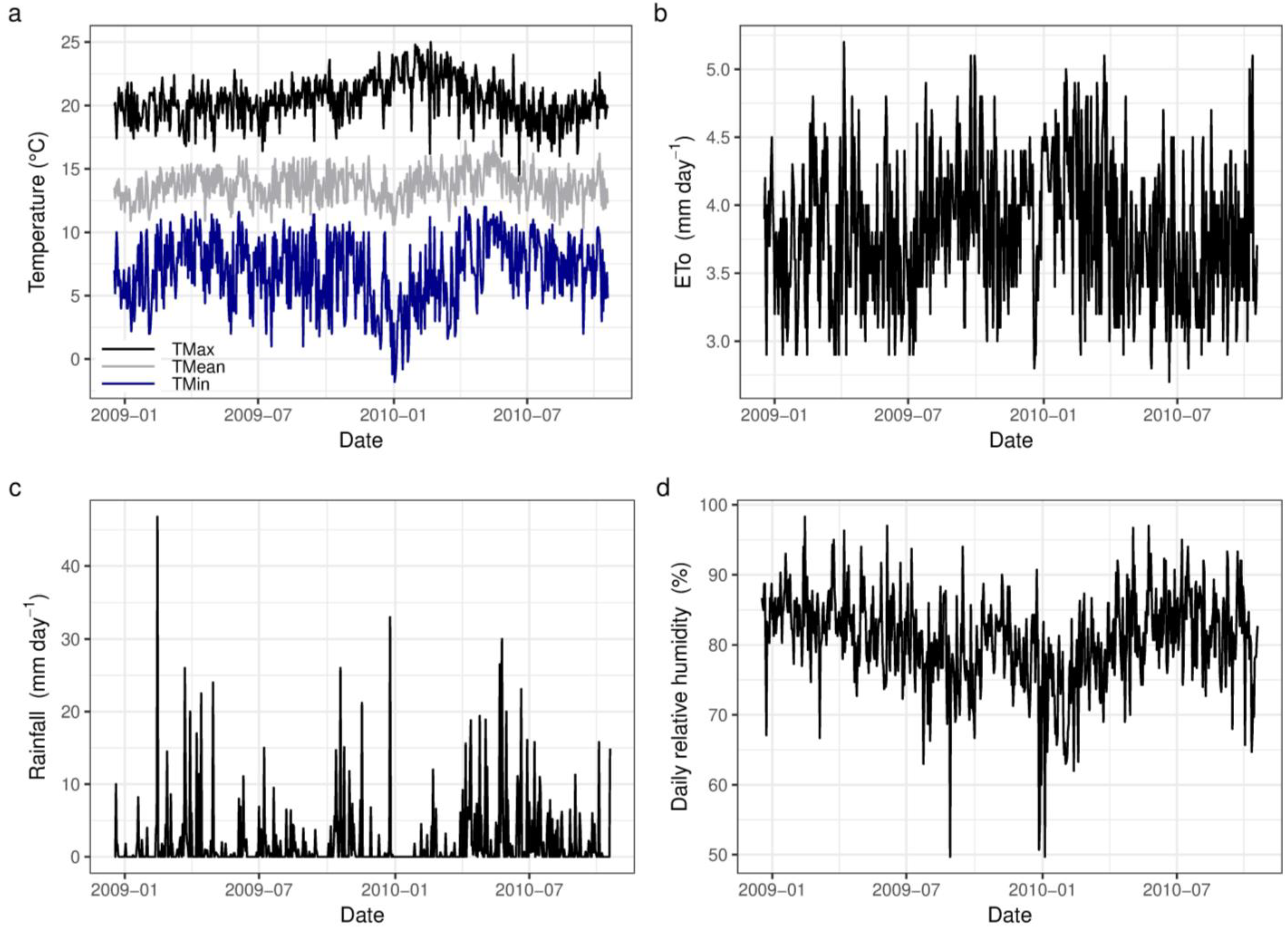
During the two growing seasons (2008–2010 and 2010) the climate data required as inputs in the AquaCrop model were collected. The minimum climate variables required for AquaCrop include daily, decadal, or monthly minimum and maximum air temperature, solar radiation, relative humidity, wind velocity, reference evapotranspiration (ET₀), and precipitation. Daily meteorological data were obtained from a meteorological station, located at the experimental site, which is part of the network of meteorological stations of the Institute of Hydrology, Meteorology, and Environmental Studies (IDEAM) of Colombia. Reference evapotranspiration was calculated following the modified Penman-Monteith equation [32] using ET₀ Calculator FAO version 3.2 [33]. A default file of the annual mean CO₂ concentration measured at the Mauna Loa Observatory in Hawaii provided by AquaCrop was used.

Figure 1 shows the meteorological air temperature, reference evapotranspiration (ET₀), precipitation, and relative humidity on a daily basis during the two seasons or experimental cycles. The first season (2008–2010) consisted of a normal year, with 624 mm (5% below the historical average); in contrast, precipitation during the 2010 season was 1054 mm (61% above the historical annual average). During this period, Colombia experienced a strong cold phase of El Niño Southern Oscillation (ENSO) known as “La Niña”. This event was one of the most intense on record, both in duration and magnitude. From July 2010, positive anomalies were consolidated, which initiated the cold event and lasted 18 months, until December 2011 [34].

Regarding reference evapotranspiration, which is the main input climate component in the AquaCrop model, the temporal pattern of ET₀ is representative of the Colombian high tropics, with an average annual accumulated ET₀ of 890 mm. The lowest ET₀ values occurred during November and December (2.7 mm day ⁻¹) and the highest values occurred during September and October (5.2 mm day ⁻¹).

2.5.2. Soil Data

Unaltered soil samples were taken to determine the moisture retention curves. Based on these results, the usable water table and hydrodynamic soil levels such as Permanent Wilt Point (PWP) and Field Capacity (FC), Saturation Point (Sat) and Hydraulic Conductivity, as well as bulk density (Da) were calculated. FC and PWP were determined via the thermo-gravimetric method; we verified using the indicator plant method for sunflower (Helianthus annuus) [35]. The creation of the soil file in AquaCrop (SOL) required soil hydraulic parameters (

Table 2. Physical characteristics of the soil in the experimental site.

Soil Depth (m)	${\mathit{\rho }}_{\mathit{b}}$ g cm−3	Suction (Mpa)							FC % Vol	PWP % Vol	TAW		SHC
		0	0	0.01	0.03	0.1	0.3	1.5			% Vol	Water Depth mm m−1	mm day−1
		% Grav	% Vol	Volumetric Soil Water Content (%)
0–30	0.85	70.60	60.01	58.30	46.16	31.58	27.29	20.68	46.16	20.68	25.48	76.44	226.45
30–60	0.92	71.09	63.83	62.22	50.66	34.99	29.67	20.97	50.66	20.97	29.69	89.07	317.63

Notes: ${\rho }_b$ is bulk density; SWRC is soil water retention curve; FC is field capacity; PWP denotes the permanent wilting point; TAW is total available water; SHC is saturated hydraulic conductivity.

). The soil was classified as silty loam, with 31.2% sand, 50.0% silt, and 18.8% clay. The effective depth of the root zone was 0.3 m, the field capacity (FC) was 138.48 mm, the PWP was 90.02 mm, saturation (Sat) was 180.03 mm, the saturated hydraulic conductivity (Ks) was 226.45 mm day ⁻¹, and the average soil bulk density was 0.85 g cm ⁻³. The soil of the sites is classified as Pachic Haplusstands–Humic Haplusstands–Fluventic Dystrustepts with symbols RMQa and RMQb [36]. Soil chemical properties at the experimental site were evaluated at 0.00–0.20 m depths; the chemical properties are shown in

Table 3. Chemical characteristics of the soil in the experimental site.

pH	ECe	OM	P	S	Ca	Mg	K	Fe	Cu	Mn	Zn	B
	ds m−1	%	mg kg−1	mg kg−1	cmol + kg−1	cmol + kg−1	cmol + kg−1	mg kg−1	mg kg−1	mg kg−1	mg kg−1	mg kg−1
5.70	1.39	10.91	20.60	23.52	8.21	2.26	0.86	623	3.4	10.9	45	0.2

Notes: ECe is electrical conductivity; OM is organic matter; P is available phosphorus; S is available sulfur; Ca is available calcium; Mg is available magnesium; K is available potassium; Fe is available iron; Cu is available copper; Zn is available zinc; B is available boron.

.

2.5.3. Crop Data

Growth was monitored daily from emergence to the end of each growing season; Lolium perenne grassland was subjected to zero grazing throughout the experiment. During the productive phase, seven cuts were made in the first growing season and four cuts in the second evaluated growing season. To determine the constant dry weight and total dry matter (t ha ⁻¹), in each season, harvests were made by cutting the forage present within an area of 0.5 m × 0.5 m (0.25 m²) with three replicates at 7 cm of height above the ground. Cutting height is a major determinant of quantity and quality of stubble from which the sward will regrow in perennial glasses [37]. From each green forage sample, a subsample of 500 g was taken and placed in paper bags in a drying oven at a temperature of 60 °C for 72 h. All samples were weighed with a precision scale (0.001 g) to determine the fresh and dry weight.

Table 4. Observed dry-matter production, plant height, irrigation, and days after planting (DAP) for the different cuttings of ryegrass (Lolium perenne L.) in the two cropping seasons (2008–2010).

Cut ID	DAP	Treatment	Plant Height (cm)		Dry Matter Production (t ha−1)		Rainfall (mm)	Irrigation (mm)
			Mean	±sd	Mean	±sd		Mean	±sd
1	88	C1-Irrigation	80.91	6.07	6.18	1.64	134.00	113.07	3.17
		C1-Non Irrigated	59.83	13.79	4.61	1.27	134.00	-	-
2	138	C1-Irrigation	76.08	7.21	4.94	1.13	168.60	33.57	2.83
		C1-Non Irrigated	44.76	4.72	1.89	0.39	168.60	-	-
3	188	C1-Irrigation	60.54	7.63	5.09	0.94	37.80	88.20	2.34
		C1-Non Irrigated	43.45	6.39	3.07	0.28	37.80	-	-
4	265	C1-Irrigation	81.35	4.85	6.09	1.43	87.90	129.13	4.32
		C1-Non Irrigated	47.18	4.73	2.54	0.74	87.90	-	-
5	320	C1-Irrigation	66.30	4.59	6.19	0.98	124.60	63.95	2.45
		C1-Non Irrigated	33.18	3.36	1.71	0.34	124.60	-	-
6	363	C1-Irrigation	56.69	9.72	4.24	0.83	47.80	64.53	3.21
		C1-Non Irrigated	36.59	7.27	2.45	0.39	47.80	-	-
7	410	C1-Irrigation	39.90	4.9	4.28	0.81	39.70	152.00	5.55
		C1-Non Irrigated	26.66	4.43	2.87	0.82	39.70	-	-
8	90	C2-Irrigation	108.34	3.26	9.75	1.14	218.90	180.33	7.42
		C2-Non Irrigated	64.49	10.83	7.58	0.72	218.90	58.04	7.78
9	146	C2-Irrigation	102.40	4.78	7.11	1.4	242.00	5.00	0.93
		C2-Non Irrigated	77.16	12.68	6.19	1.95	242.00	-	-
10	191	C2-Irrigation	83.54	6.95	3.77	0.85	105.50	-	-
		C2-Non Irrigated	76.81	12.76	3.33	1,00	105.50	-	-
11	239	C2-Irrigation	66.91	5.73	4.13	0.86	70.30	45.53	4.76
		C2-Non Irrigated	51.24	4.79	4.01	0.35	70.30	-	-

Notes: ±sd is standard deviation; C1-Irrigation: full irrigation treatment in the first cropping season of ryegrass (December 2008 to January 2010); C1-Non-Irrigated: non-irrigated treatment in the first cropping of season ryegrass (December 2008 to January 2010); C2-Irrigation: full irrigation treatment in the second cropping season of ryegrass (February 2010 to October 2010); C2-Non-Irrigated: non-irrigated treatment in the second cropping season of ryegrass (February 2010 to October 2010).

shows an overview of the mean dry matter biomass weights observed for each cutting, plant height, and water supply condition.

Canopy cover was obtained from photographs taken at 1.4 m from the ground with a digital camera. The image was processed in CobCal v2.1 software [38], where the user marks the colors of the pixels corresponding to the vegetation cover as positive pixels and the colors corresponding to the ground as negative pixels. Subsequently, the pixels are sorted by Euclidean distance, and the percentage of cover is calculated by counting the number of pixels corresponding to each group.

The AquaCrop crop files were created based on field observations of crop development and phenology. The AquaCrop model uses conservative and non-conservative parameters for the simulation. Conservative parameters do not change with location, management, cultivars, and time [39]. Conservative parameters must be adjusted to improve the simulations in the model [40]. They include canopy cover (CC), canopy growth coefficient (CGC), canopy decline coefficient (CDC), crop coefficient for transpiration at full CC, and normalized water productivity (WP*) for biomass formation. Crop water stress parameters (soil water depletion thresholds for leaf growth inhibition and stomatal conductance and for acceleration of canopy senescence) were taken from Terán-Chaves et al. [41]. The crop parameters were iteratively adjusted with the help of the Independent Parameter Estimation Model (PEST) Ver. 5. [42] (PEST is an acronym for ESTimation of Parameter) until a close match between measured and simulated parameters was achieved.

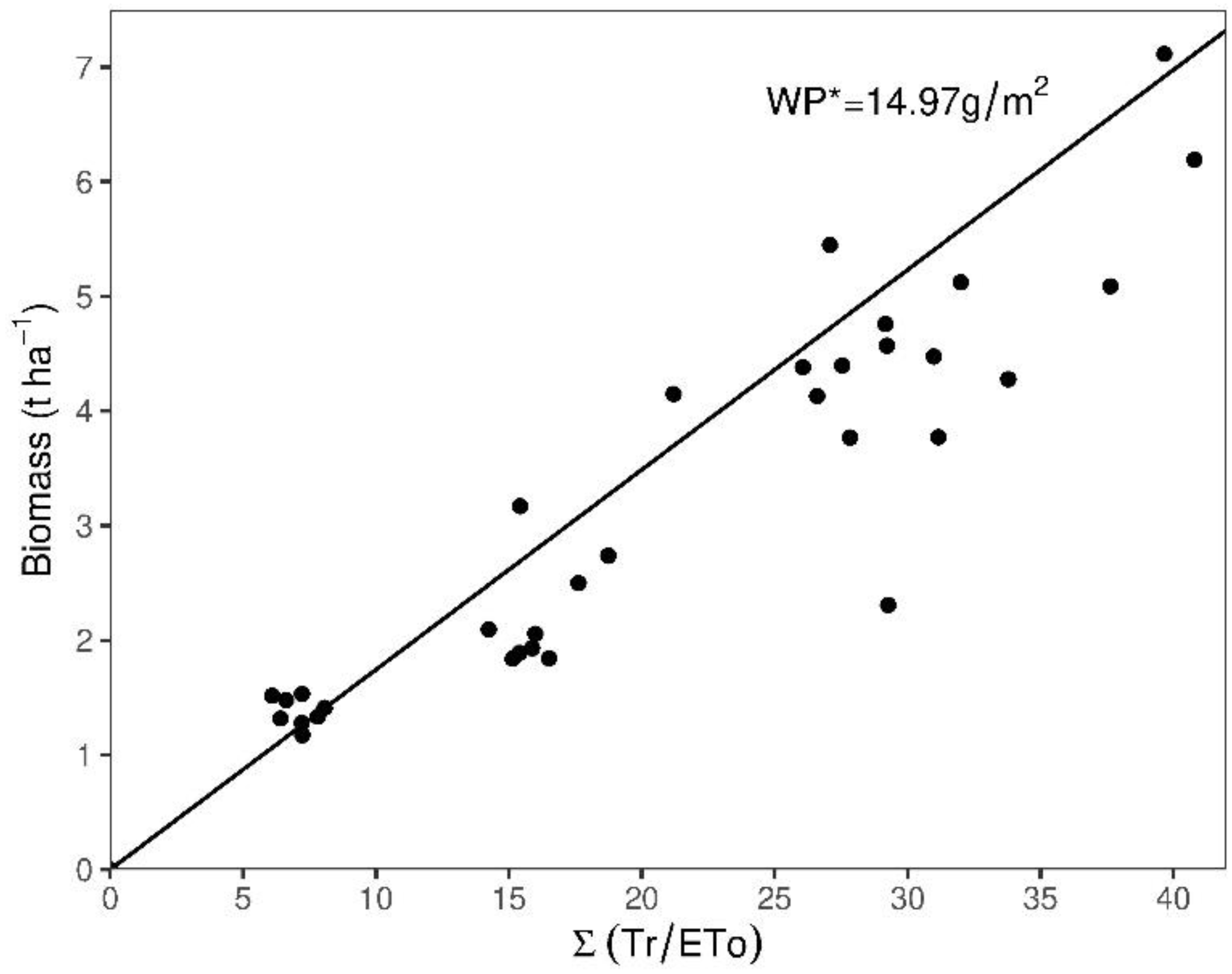
Water productivity (WP) for biomass production was determined as the ratio of biomass to actual accumulate transpiration [43]. The initial value of WP* was obtained as the slope of the linear regression of a plot of biomass accumulation versus accumulated transpiration values normalized to ET₀, i.e., ∑Tr/ET₀.

2.6. Model Calibration and Validation

AquaCrop version 7.0 (2022) [44] was used; the model was run in calendar days, and the perennial herbaceous forage crop file of alfalfa was taken as a reference. The standard window version 7.0 user interface included a database of perennial herbaceous forage crops, with multiple harvests, the amount of biomass, and crop yield harvested at each cut during the growing cycle in case of multiple cuttings; these data were stored in a ‘harvests’ output file. In this study, the calibration and validation guidelines described by Hsiao et al. were followed [31]; data from the non-limiting soil water regime treatment (C1-Irrigation: full irrigation treatment in the first cropping season of ryegrass) were used to calibrate AquaCrop. The calibration process was performed by running the model with the specific input information of weather conditions, soil characteristics, field managements practice, and crop parameters. The calibration also involved adjusting the non-conservative parameters, including initial canopy cover CCo (%), maximum canopy cover (CCx), time from sowing to start of senescence (day), and maximum effective rooting depth (m), until a close match between observed and simulated biomass was obtained.

For the first stage, from sowing to first cutting, the soil surface cover of an individual seed at 90% emergence observed in the field and the final yield at the time of cutting were taken into account. For cuts after the first cut, the canopy cover after cutting (CCini) was specified at a value of 40% according to field measurements.

Once the model was successfully calibrated, it was validated using three independent datasets obtained from the experiment, namely C1-Non-Irrigated: non-irrigated treatment in the first cropping season of ryegrass (December 2008 to January 2010), C2-Irrigation: full irrigation treatment in the second cropping season of ryegrass (February 2010 to October 2010), and C2-Non-Irrigated: non-irrigated treatment in the second cropping season of ryegrass (February 2010 to October 2010).

2.7. Model Evaluation Statistics

The goodness-of-fit of the AquaCrop model for ryegrass was evaluated using the following five statistics: the coefficient of determination (R²), the Willmott index of agreement (d-index), the root mean square error (RMSE), the normalized root mean square error (NRMSE), and the Nash-Sutcliffe model efficiency coefficient (EF). The evaluations of simulation results were recorded in statistics output files. The output files contain the statistics of the evaluation of the simulation results for canopy cover, biomass, and soil water content.

According to FAO [45] for R², (Equation (3)) values > 0.90 were considered to be very good, while values between 0.70 and 0.90 were considered to be good. Values between 0.50 and 0.70 were considered to be moderately good, while values below 0.50 were considered to be poor. The d-index (Equation (4)) ranges from 0 to 1, where 0 indicates no agreement and 1 indicates perfect agreement between simulated and observed data; the d-index was acceptable when it was above 0.64. RMSE (Equation (5)) varies from 0 to positive infinity and is expressed in units of the studied variable. An RMSE close to 0 indicates good model performance. The NRMSE (Equation (6)), on the other hand, gives an indication of the relative difference between the simulated and observed values. NRMSE < 5% is considered very good; 6~15% is good; 16~25% is moderately good, 16~25% is moderately poor, and NRMSE > 26% is poor [46]. The efficiency coefficient of the Nash–Sutcliffe (EF) model (Equation (7)) determines the relative magnitude of the residual variance, compared to the variance of the observations. An EF indicates how good the fit of the plot of observed vs. simulated data is on the 1:1 line; it ranges from minus infinity to one. One means a perfect fit, and zero indicates that the model predictions are as accurate as the average of the observed data and negative when the mean of the observations is less than the model predictions. An EF less than 0.4 is considered deficient. The simulation results were considered good when at least three of the five statistical fit indicators of the model evaluation were classified as good to very good.

$${\mathrm{R}}^2={\left(\frac{{{\displaystyle \sum }}_{i=1}^n\left(O_i-\overline{O}\right) \left(P_i-\overline{P}\right)}{\sqrt{{{\displaystyle \sum }}_{i=1}^n{\left(O_i-\overline{O}\right)}^2}\sqrt{{{\displaystyle \sum }}_{i=1}^n{\left(P_i-\overline{P}\right)}^2 }}\right)}^2$$

(3)

$$\mathrm{d}=1-\frac{{{\displaystyle \sum }}_{i=1}^n{\left(P_i-O_i\right)}^2}{{{\displaystyle \sum }}_{i=1}^n{\left(\left|P_i-\overline{O}\right|+\left|O_i-\overline{O}\right|\right)}^2}$$

(4)

$$\mathrm{RMSE}=\sqrt{\frac{{{\displaystyle \sum }}_{i=1}^n{\left(P_i-O_i\right)}^2}{n}}$$

(5)

$$\mathrm{NRMSE}=\frac{1}{\overline{O}} \sqrt{\frac{{{\displaystyle \sum }}_{i=1}^n{\left(P_i-O_i\right)}^2}{n}}\ast 100$$

(6)

$$\mathrm{EF}=1-\frac{{{\displaystyle \sum }}_{i=1}^n{\left(P_i-O_i\right)}^2}{{{\displaystyle \sum }}_{i=1}^n{\left(O_i-\overline{O}\right)}^2}$$

(7)

where $O_i$ = is the observed data; $\overline{O}=$ is the average of observed data; $P_i=$ is the simulated data; $\overline{P}=$ is the average of simulated data; and n is the observation number.

3. Results

3.1. Calibration of the AquaCrop Model for Soil, Green Canopy Cover, Dry Matter, and Water Content

Table 5. Detailed AquaCrop Ryegrass (Lolium perenne L.): conservative and/or crop specific parameters.

Crop Parameter	Value	Method of Determination
Base temperature (°C)	4	L
Upper temperature (°C)	35	L
Soil water depletion factor for canopy expansion (p-exp)—Upper threshold	0.98	M
Soil water depletion factor for canopy expansion (p-exp)—Lower threshold	0.25	M
Shape factor for water stress coefficient for canopy expansion	10.8	M
Soil water depletion fraction for stomatal control (p-sto)—Upper threshold	0.5	M
Shape factor for water stress coefficient for stomatal control	4.2	M
Soil water depletion factor for canopy senescence (p-sen)—Upper threshold	0.3	C
Shape factor for water stress coefficient for canopy senescence	2.5	C
Vol% for anaerobiotic point ((SAT—[vol%]) at which deficient aeration occurs)	−12	M
Canopy growth coefficient (CGC): Increase in canopy cover (fraction soil cover per day)	0.1086	M
Canopy decline coefficient (CDC): Decrease in canopy cover (in fraction per day)	0.0143	M
Crop coefficient when canopy is complete but prior to senescence (Kc,Tr,x)	1	M
Water productivity normalized for ET0 and CO2 (WP*) (g/m2)	14.7	M

Notes: C: calibration; E: estimation; L: literature; M: measured.

presents the conservative parameters, which are crop-specific and largely independent of management or agroclimatic zone [31].

Table 6. Detailed AquaCrop Ryegrass (Lolium perenne L.): non-conservative and/or cultivar-specific parameters.

Crop Parameter	Value	Method of Determination
Time to reach 90% crop emergence (days) for the first cut	9	M
Time to reach 90% crop emergence (days) after the first cutting	6	M
Time to reach 90% crop emergence (growing degree days) for the first cut	84–91	M
Time to reach 90% crop emergence (growing degree days) after the first cutting	25–87	M
Calendar days from sowing to maximum rooting depth	64	M
Degree days from sowing to maximum rooting depth	604	M
GDD from sowing to flowering for the first cut (growing degree days)	795–803	M
Calendar days from sowing to flowering (days)	83	M
Calendar days from sowing to flowering (days) after the first cutting	44	M
GDD from sowing to flowering after the first cutting (growing degree days)	418–426	M
Calendar days from sowing to maturity (length of crop cycle) for the first cut	100	M
GDD from sowing to maturity (length of crop cycle) for the first cut (growing degree days)	970–974	M
Calendar days from sowing to maturity (length of crop cycle) after the first cutting	55	M
GDD from sowing to maturity (length of crop cycle) after the first cutting (growing degree days)	530–540	M
Minimum effective rooting depth (m)	0.06	M
Maximum effective rooting depth (m)	0.4	M
Shape factor describing root zone expansion	1	E
Maximum root water extraction (m3 water/m3 soil.day) in top quarter of root zone	0.020	E
Maximum root water extraction (m3 water/m3 soil.day) in bottom quarter of root zone	0.010	E
Effect of canopy cover in reducing soil evaporation in late season stage	50	M
Soil surface covered by an individual seedling at 90% emergence (cm2) for first cut	0.76	M
Soil surface covered by an individual seedling at 90% emergence (cm2) after the first cutting	3.67	M
Number of plants per hectare	11,600,000	M
Number of plants per m2	1160	M
Maximum canopy cover (CCx) in fraction soil cover	0.97	M
Reference Harvest Index (HIo) (%)	100	D

Notes: D: AquaCrop default; E: estimation; L: literature; M: measured.

proposes non-conservative parameters, i.e., crop-dependent parameters, which were successfully calibrated and validated in the present study but may vary according to cultivar and location [46].

For the dataset used, CO₂-normalised biomass measurements were plotted against cumulative normalized transpiration (∑Tr/ET₀), with a slope of the regression line (equivalent to WP*) of 14.97 g m⁻² and an R² of 0.97 (Figure 2). The WP* value is in the range of values for C3 crops (13–18 g m⁻²) [47].

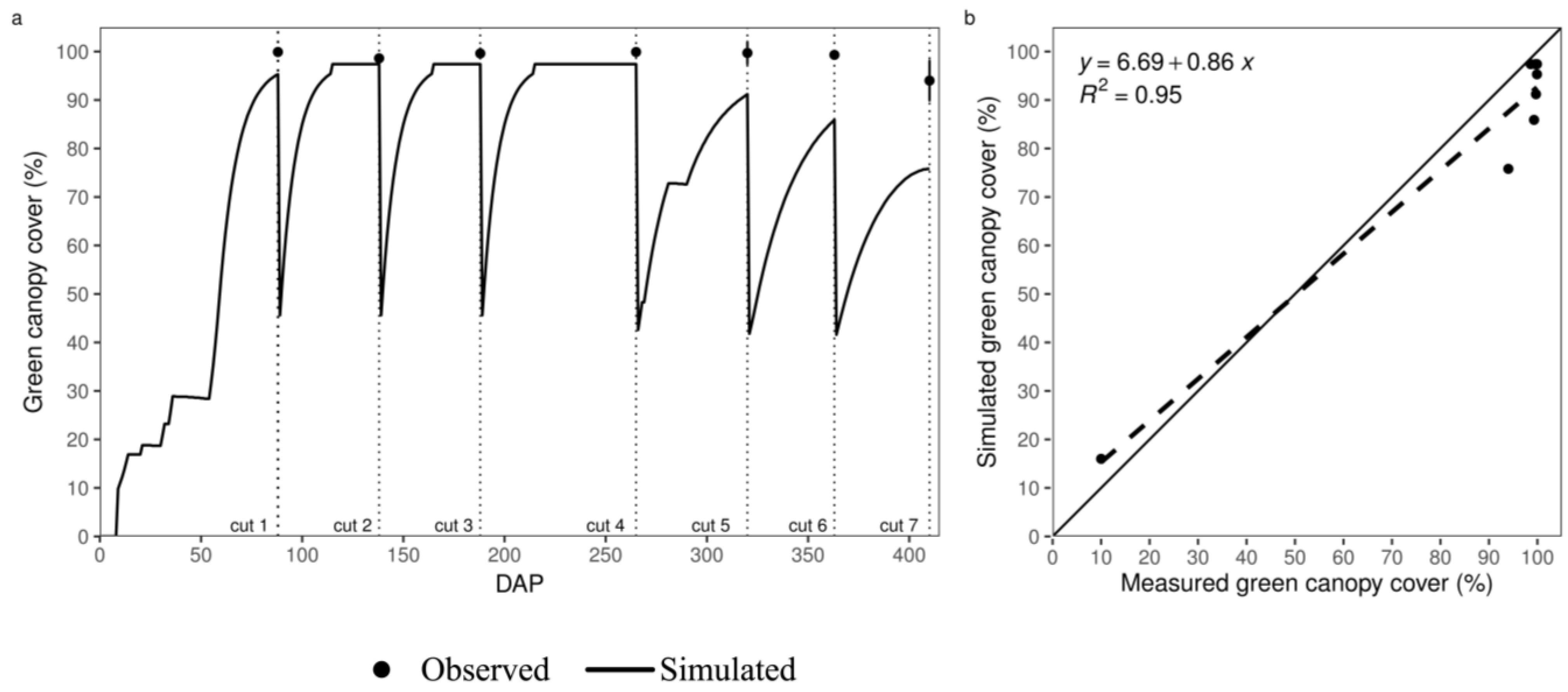
In the calibration, the parameter values adopted for the canopy cover simulation (Figure 3) presented a good goodness-of-fit (R² = 0.95, d-index = 0.41, RMSE = 9.4%, NRMSE = 12.2%, and EF = −21.72). The simulation of CC throughout crop development shows a slight tendency of underestimation in cuts 5, 6, and 7.

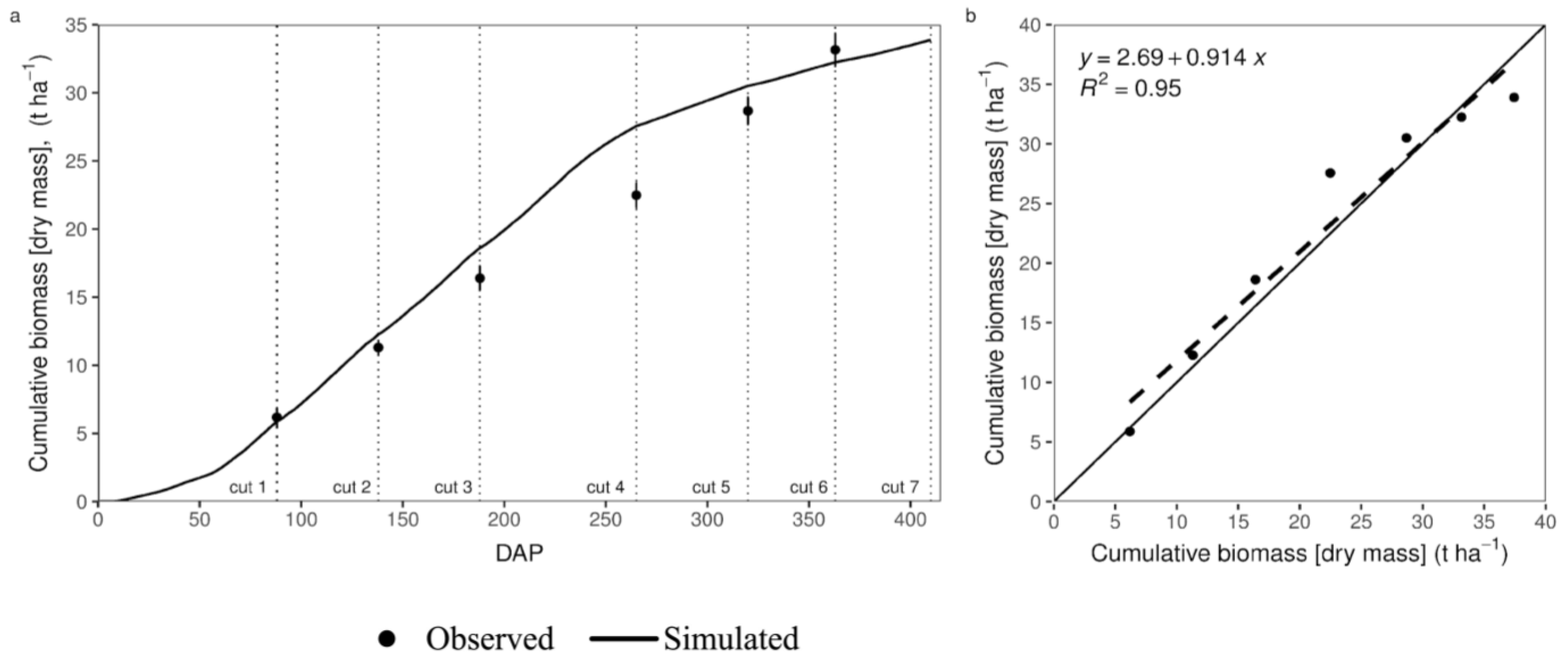
Dry matter production was monitored using seven cuts during the 2008–2010 growing season. AquaCrop, in its recent incorporation of herbaceous forage crops, performs goodness-of-fit calculations per (dry matter) biomass accumulated after each defoliation made to the crop; for this reason, Figure 4 shows the comparisons of observed and simulated biomass accumulated after each cutting. Although the linear correlation between observed and simulated values presented a high correlation coefficient (R² = 0.95), the model underestimated the biomass obtained in cuts 5, 6, and 7 and compensated by overestimating the production in cut 4. The different values of the statistical indices reveal that their interpretation strongly depends on the overall performance of the model in simulating the accumulated biomass and not by cutting or defoliation done on forage crops. The statistical indicators showed a very good performance for accumulated biomass (R² = 0.95, d-index = 0.98, RMSE = 2.63 t ha⁻¹, NRMSE = 11.8%, and EF = 0.94).

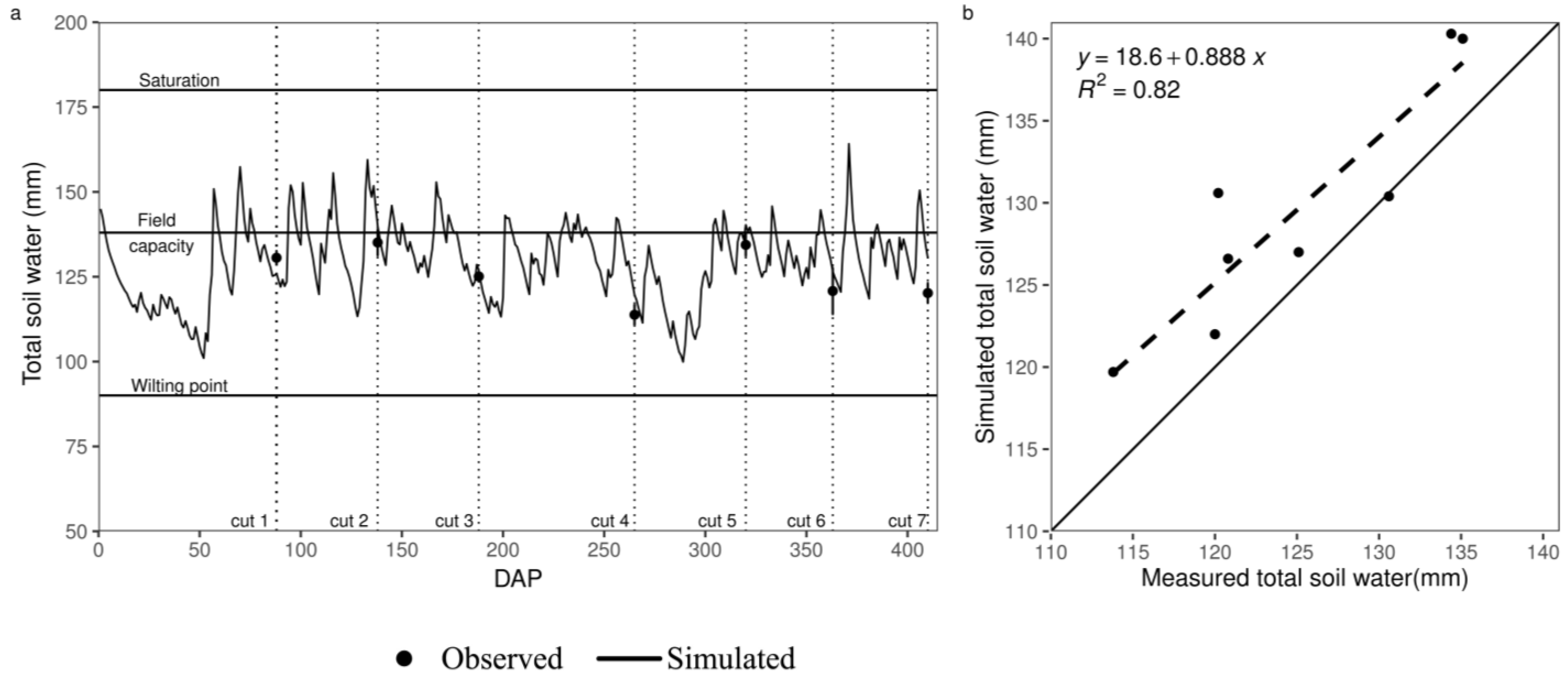
The irrigation simulation model can be evaluated through the dynamics of soil water content, which are based on field observations (Figure 5). Water availability around roots is critical for driving transpiration, which is directly proportional to biomass. AquaCrop simulated soil water content with reasonable accuracy (R² = 0.82, d-index = 0.84, RMSE = 6.10 mm, NRMSE = 4.80%, and EF = 0.32).

3.2. AquaCrop Model Validation for Ryegrass Crop (Lolium perenne L.)

Model validation was conducted using calibrated crop parameters obtained from a dataset with three treatments not used for calibration. Statistical parameters of fit for all treatments and variables are presented in

Table 7. Statistical evaluation parameters and values for green canopy cover, cumulative biomass dry matter, and soil water, for calibration and validation treatments of ryegrass (Lolium perenen L.).

Statistics	C1-Irrigation	C1-Non Irrigated	C2-Irrigation	C2-Non Irrigated
	Calibration	Validation	Validation	Validation
Green Canopy Cover (%)
R2	0.95	0.42	1.00	0.92
d	0.41	0.01	0.84	0.96
RMSE (%)	9.40	40.60	16.80	7.40
NRMSE (%)	9.50	40.90	23.00	8.50
EF	−21.72	−25.71	0.61	0.82
Cumulative Biomass Dry Matter (t ha−1)
R2	0.95	0.91	1.00	1.00
d	0.98	0.91	0.99	0.92
RMSE (t ha−1)	2.63	2.87	1.43	3.50
NRMSE (%)	11.80	24.50	8.00	23.10
EF	0.94	0.65	0.93	0.52
Total Soil Water (mm)
R2	0.82	0.86	0.83	0.83
d	0.84	0.75	0.73	0.30
RMSE (mm)	6.10	20.00	7.70	20.10
NRMSE (%)	4.80	24.10	6.20	17.50
EF	0.32	−0.03	−1.14	−23.96

Notes: C1-Irrigation: full irrigation treatment in the first cropping season of ryegrass (December 2008 to January 2010); C1-Non-Irrigated: non-irrigated treatment in the first cropping season of ryegrass (December 2008 to January 2010); C2-Irrigation: full irrigation treatment in the second cropping season of ryegrass (February 2010 to October 2010); C2-Non-Irrigated: non-irrigated treatment in the second cropping season of ryegrass (February 2010 to October 2010).

. AquaCrop underestimated canopy cover for C1-Non-Irrigated treatment (R² = 0.42, d-index = 0.01, RMSE = 40.60%, NRMSE = 40.90%, and EF = −25.71). Specifically, for ryegrass under water stress during the first evaluated season, the model underestimated ryegrass canopy expansion from cut 3 to cut 7, reducing canopy cover on average by 47%. For the C2-Non-Irrigated treatment, the model performed well (R² = 0.92, d-index = 0.96, RMSE = 7.40%, NRMSE = 8.50%, and EF = 0.82). It is important to mention that despite this being a non-irrigated treatment, during this second crop season, Colombia experienced unusually high rainfall, which kept soil moisture in acceptable conditions and the crop did not experience water stress. Overall, the statistical indicators suggest that AquaCrop was able to accurately simulate CC for the other treatments considered in the validation phase.

Cumulative biomass values from the model closely matched values from the validation treatments: C1-Non-Irrigated (R² = 0.91, d-index = 0.91, RMSE = 2.87 t ha⁻¹, NRMSE = 24.50%, and EF = 0.65), C2-Irrigation (R² = 1.0, d-index = 0.99, RMSE = 1.43 t ha⁻¹, NRMSE = 8.0%, and EF = 0.93) and C2-Non-Irrigated (R² = 1.0, d-index = 0.92, RMSE = 3.5 t ha⁻¹, NRMSE = 23.1%, and EF = 0.52). Considering the yield indices reported in Table 6, the model appears properly calibrated for biomass.

Simulations of soil water content correlated strongly with values from the validation treatments, namely C1-Non-Irrigated (R² = 0.86, d-index = 0.75, RMSE = 20 mm, NRMSE = 24.10%, and EF = −0.03), C2-Irrigation (R² = 0.83, index d = 0.73, RMSE = 7.7 mm, NRMSE = 6.20%, and EF = −1.14) and C2-Non-Irrigated (R² = 0.83, index d = 0.30, RMSE = 20.10 mm, NRMSE = 17.50%, and EF = −23.96). It should be noted that for all treatments a negative EF was obtained, which implies that the mean of the observations provides a better prediction than the model. Positive EF values constitute the minimum acceptance criteria for simulating soil water content in crop models [48]. Nevertheless, the other statistical parameters demonstrate that AquaCrop was able to simulate soil water dynamics with reasonable accuracy in this study.

4. Discussion

To date, forage grass models have been developed to simulate perennial ryegrass growth processes under temperate climates [49,50]; hence, they cannot be used for predicting grassland productivity in tropical regions such as Colombia. This study is, to our knowledge, the first to calibrate and validate the AquaCrop model for perennial ryegrass (Lolium perenne L.) using version 7.0.

The results showed that the AquaCrop (v 7.0) model was able to simulate perennial ryegrass growth under normal and wet seasons in the high tropic of Colombia. This capacity may allow many future applications for tropical pasture species with high importance for livestock or the production of energy from biomass. However, the capacity of the AquaCrop model for simulating the effect of grazing on late regrowth pasture and its effects on canopy cover and biomass must be further studied.

The model simulated canopy cover growth well from first cut to fourth cut; however, after the fifth cut, a rapid decline in canopy cover was generated instead of the gradual decline rate observed in the field, which could be attributed to the indeterminate growth characteristic of perennial ryegrass. Previous studies have identified this limitation of the AquaCrop model in crops exhibiting indeterminate growth characteristics [51,52,53]. AquaCrop does not consider leaf appearance rate or phyllochron; this may explain the underestimation of the simulated values. The potential growth rate of the leaf area is proportional to the product of tiller density, the number of elongated leaves per tiller, a constant leaf width, and a temperature dependent rate of leaf elongation [11]. Most plant processes are interrupted during days when a cutting takes place; in the AquaCrop model as is in the BASGRA model, all leaf area associated with non-elongating tillers above a threshold is removed by cutting, as is the associated biomass; this also affects the development of the remaining canopy cover after the cuts.

The AquaCrop model was able to simulate biomass with acceptable accuracy under both irrigation practices, but the simulated results were observed to be slightly better suited to full irrigation practices. Full irrigation practices compensate for any lack of water from precipitation, which enables the model to quantify results with reasonable certainty.

Grazing reduces the development and growth of ryegrass reproductive tillers [54], which complicates the effects of reproductive growth on herbage accumulation, especially for late regrowth, which AquaCrop is possibly trying to simulate. To increase the accuracy of the model, the effect of grazing on the growth and development of reproductive tillers needs to be incorporated, along with a more detailed simulation of plant management and phenology. The variation of pasture growth in response to irrigation was also predicted. This evaluation provided confidence in the model’s ability to simulate pasture herbage accumulation in the annual season and under various management scenarios and a wide range of pasture environments.

The importance of soil moisture deficits for ryegrass persistence was demonstrated in a modeling study by Woodward et al. [49]; soil water is important for agricultural production and is a key parameter in hydrologic models and weather prediction models. We found that AquaCrop can estimate soil moisture with acceptable precision. Soil water content was reasonably simulated, albeit simulated values had a tendency for greater variability compared with observed values. Perennial ryegrass is moderate to poorly adapted to low soil moisture availability [50]. Water shortage limits leaf appearance, leaf expansion, and tiller initiation, irrespective of the availability of other resources, and largely explains inter-annual variability in pasture growth rate [55]. Future studies should explore the sensitivity of our results to a much wider range of soil profile and available water.

5. Conclusions

The results obtained in this study show that AquaCrop is adequate in simulating the responses of perennial herbaceous forage crops to different water regimes; however, the goodness-of-fit evaluation of AquaCrop v 7.0 for crops with multiple harvests during a single season should be generated for each harvest or cutting and not as a cumulative biomass value as is currently presented.

Additional experiments are needed to adjust the parameters developed in this study to account for other environmental conditions and to properly estimate biomass per cutting. In the meantime, this study serves as a baseline for further modeling of perennial herbaceous forage crops with AquaCrop version 7.0 and newer.

Future modeling studies of perennial herbaceous forage crops should delve further into the comparison of soil moisture content simulations under various irrigation practices and climatic conditions. In addition, further experimentation with indeterminate crops such as ryegrass are needed to characterize a possible enveloping senescence curve, crop recovery beyond the permanent wilting point, and early canopy senescence processes due to natural causes.

References

- Dal Pizzol, J.G.; Ribeiro-Filho, H.M.N.; Quereuil, A.; Le Morvan, A.; Niderkorn, V. Complementarities between grasses and forage legumes from temperate and subtropical areas on in vitro rumen fermentation characteristics. Anim. Feed Sci. Technol. 2017, 228, 178–185. [Google Scholar] [CrossRef]
- Beechey-Gradwell, Z.; Kadam, S.; Bryan, G.; Cooney, L.; Nelson, K.; Richardson, K.; Cookson, R.; Winichayakul, S.; Reid, M.; Anderson, P.; et al. Lolium perenne engineered for elevated leaf lipids exhibits greater energy density in field canopies under defoliation. Field Crop. Res. 2022, 275, 108340. [Google Scholar] [CrossRef]
- Ovalle, C.; Del Pozo, A.; Peoples, M.B.; Lavín, A. Estimating the contribution of nitrogen from legume cover crops to the nitrogen nutrition of grapevines using a 15N dilution technique. Plant Soil 2010, 334, 247–259. [Google Scholar] [CrossRef]
- Santos-Torres, M.; Romero-Perdomo, F.; Mendoza-Labrador, J.; Gutiérrez, A.Y.; Vargas, C.; Castro-Rincon, E.; Caro-Quintero, A.; Uribe-Velez, D.; Estrada-Bonilla, G.A. Genomic and phenotypic analysis of rock phosphate-solubilizing rhizobacteria. Rhizosphere 2021, 17, 100290. [Google Scholar] [CrossRef]
- MADR—Ministry of Agriculture and Rural Development of Colombia. Cadena Láctea Colombiana. In Principales Desafíos del Análisis Situacional; Bogotá, Colombia, 2020. Available online: https://www.upra.gov.co/documents/10184/124468/20200820_PPT_Analisis_Situacional_CadenaLactea.pdf/415b9312-a13b-4061-84f5-fd83c1b48dbc (accessed on 20 October 2022).
- Didiano, T.J.; Johnson, M.T.J.; Duval, T.P. Disentangling the Effects of Precipitation Amount and Frequency on the Performance of 14 Grassland Species. PLoS ONE 2016, 11, e0162310. [Google Scholar] [CrossRef] [PubMed]
- Thébault, A.; Mariotte, P.; Lortie, C.; MacDougall, A. Land management trumps the effects of climate change and elevated CO2 on grassland functioning. J. Ecol. 2014, 102, 896–904. [Google Scholar] [CrossRef]
- Tubiello, F.N.; Soussana, J.F.; Howden, S.M. Crop and pasture response to climate change. Proc. Natl. Acad. Sci. USA 2007, 104, 19686–19690. [Google Scholar] [CrossRef] [PubMed] [Green Version]
- Jing, Q.; Qian, B.; Bélanger, G.; VanderZaag, A.; Jégo, G.; Smith, W.; Grant, B.; Shang, J.; Liu, J.; He, W.; et al. Simulating alfalfa regrowth and biomass in eastern Canada using the CSM-CROPGRO-perennial forage model. Eur. J. Agron. 2020, 113, 125971. [Google Scholar] [CrossRef]
- Institute of Hydrology, Meteorology and Environmental Studies of Colombia—IDEAM. Tercera Comunicación Nacional de Cambio Climático. 2017. Available online: http://documentacion.ideam.gov.co/openbiblio/bvirtual/023731/TCNCC_COLOMBIA_CMNUCC_2017_2.pdf (accessed on 24 September 2022).
- Höglind, M.; Van Oijen, M.; Cameron, D.; Persson, T. Process-based simulation of growth and overwintering of grassland using the BASGRA model. Ecol. Model. 2016, 335, 1–15. [Google Scholar] [CrossRef] [Green Version]
- Schapendonk, A.; Stol, W.; Kraalingen, D.; Bouman, B. LINGRA, a sink/source model to simulate grassland productivity in Europe. Eur. J. Agron. 1998, 9, 87–100. [Google Scholar] [CrossRef]
- Riedo, M.; Grub, A.; Rosset, M.; Fuhrer, J. A pasture simulation model for dry matter production, and fluxes of carbon, nitrogen, water and energy. Ecol. Model. 1998, 105, 141–183. [Google Scholar] [CrossRef]
- Li, F.Y.; Snow, V.O.; Holzworth, D.P.; Johnson, I.R. Integration of a pasture model into APSIM. In Proceedings of the 13th Australian Agronomy Conference, Lincoln, New Zealand, 15–19 November 2010; Available online: www.regional.org.au/au/asa/2010/farming-systems/simulation-decisionsupport/6993_lifyrevis.htm (accessed on 5 July 2022).
- Vogeler, I.; Cichota, R. Deriving seasonally optimal nitrogen fertilization rates for a ryegrass pasture based on agricultural production systems simulator modelling with a refined AgPasture model. Grass Forage Sci. 2015, 71, 353–365. [Google Scholar] [CrossRef]
- Araujo, L.C.; Santos, P.M.; Rodriguez, D.; Pezzopane, J.R.M.; Oliveira, P.P.; Cruz, P.G. Simulating Guinea grass production: Empirical and mechanistic approaches. Agron. J. 2013, 105, 61–69. [Google Scholar] [CrossRef] [Green Version]
- Bosi, C.; Sentelhas, P.C.; Huth, N.I.; Pezzopane, J.R.M.; Andreucci, M.P.; Santos, P.M. APSIM-Tropical Pasture: A model for simulating perennial tropical grass growth and its parameterisation for palisade grass (Brachiaria brizantha). Agric. Syst. 2020, 184, 102917. [Google Scholar] [CrossRef]
- Rymph, S.J. Modulen voor de Lerarenopleiding Basisonderwijs; Amsterdam University Press: Amsterdam, The Netherlands, 2004. [Google Scholar]
- Pedreira, B.C.; Pedreira, C.G.S.; Boote, K.J.; Lara, M.A.S.; Alderman, P.D. Adapting the CROPGRO perennial forage model to predict growth of Brachiaria brizantha. Field Crop. Res. 2011, 120, 370–379. [Google Scholar] [CrossRef]
- Dos Santos, M.L.; Santos, P.M.; Boote, K.J.; Pequeno, D.N.L.; Barioni, L.G.; Cuadra, S.V.; Hoogenboom, G. Applying the CROPGRO Perennial Forage Model for long-term estimates of Marandu palisadegrass production in livestock management scenarios in Brazil. Field Crop. Res. 2022, 286, 108629. [Google Scholar] [CrossRef]
- Raes, D.; Steduto, P.; Hsiao, T.C.; Fereres, E. AquaCrop—The FAO Crop Model to Simulate Yield Response to Water: II. Main Algorithms and Software Description. Agron. J. 2009, 101, 438–447. [Google Scholar] [CrossRef] [Green Version]
- Vanuytrecht, E.; Raes, D.; Steduto, P.; Hsiao, T.C.; Fereres, E.; Henge, L.K.; Vila, M.G.; Moreno, P.M. AquaCrop: FAO’s crop water productivity and yield response model. Environ. Model. Softw. 2014, 62, 351–360. [Google Scholar] [CrossRef]
- Kim, D.; Kaluarachchi, J. Validating FAO AquaCrop using Landsat images and regional crop information. Agric. Water Manag. 2015, 149, 143–155. [Google Scholar] [CrossRef]
- Terán-Chaves, C.A. Determinación de la Huella Hídrica y Modelación de la Producción de Biomasa de Cultivos Forrajeros a Partir del Agua en la Sabana de Bogotá (Colombia). Ph.D. Thesis, Universitat Politècnica de València, Valencia, Spain, 2015. [Google Scholar] [CrossRef]
- Stricevic, R.; Simic, A.; Kusvuran, A.; Cosic, M. Assessment of AquaCrop model in the simulation of seed yield and biomass of Italian ryegrass. Arch. Agron. Soil Sci. 2016, 63, 1301–1313. [Google Scholar] [CrossRef]
- Steduto, P.; Hsiao, T.C.; Raes, D.; Fereres, E. AquaCrop-The FAO Crop Model to Simulate Yield Response to Water: I. Concepts and Underlying Principles. Agron. J. 2009, 101, 426–437. [Google Scholar] [CrossRef] [Green Version]
- Raes, D.; Fereres, E.; García-Villa, M.; Hsiao, T.; Kheng, L.H.; Steduto, P.; Wellens, J. AquaCrop Version 7.0—New Developments. In Proceedings of the International Symposium on Managing Land and Water for Climate Smart Agriculture, Vienna, Austria, 25–29 July 2022; Available online: https://orbi.uliege.be/bitstream/2268/295200/1/340-d.raes_abstract.pdf (accessed on 2 November 2022).
- Raes, D. AquaCrop Training Handbooks Book II.—Running AquaCrop; Food and Agriculture Organization of the United Nations: Rome, Italy, 2022; Available online: https://www.fao.org/3/i6052en/i6052en.pdf (accessed on 17 October 2022).
- Hanks, R.J.; Keller, J.; Rasmussen, V.P.; Wilson, G.D. Line source sprinkler for continuous variable irrigation-crop production studies. Soil Sci. Soc. Am. J. 1976, 40, 426–429. [Google Scholar] [CrossRef]
- Qian, Y.L.; Engelke, M.C. Performance of five turfgrasses under linear gradient irrigation. Hort. Sci. 1999, 34, 893–896. [Google Scholar] [CrossRef] [Green Version]
- Hisao, T.; Fereres, E.; Steduto, P.; Raes, D. AquaCrop Version 7.0. Chapter 4 Calibration Guidance; Food and Agriculture Organization of the United Nations, Land and Water Division: Rome, Italy, 2022; Available online: https://www.fao.org/3/br249e/br249e.pdf (accessed on 3 October 2022).
- Allen, R.G.; Pereira, L.S.; Raes, D.; Smith, M. FAO Irrigation and Drainage Paper No. 56—Crop Evapotranspiration; FAO: Rome, Italy, 1998; Available online: www.climasouth.eu/sites/default/files/FAO%2056.pdf (accessed on 10 February 2022).
- Raes, D. Reference Manual—ETo Calculator; Food and Agriculture Organization of the United Nations, Land and Water Division: Rome, Italy, 2012; Available online: https://www.fao.org/land-water/databases-and-software/eto-calculator/en/ (accessed on 3 January 2018).
- Hoyos, N.; Escobar, J.; Restrepo, J.; Arango, A.; Ortiz, J. Impact of the 2010–2011 La Niña phenomenon in Colombia, South America: The human toll of an extreme weather event. Appl. Geogr. 2013, 39, 16–25. [Google Scholar] [CrossRef]
- Taylor, S.A.; Ashcroft, G.L. Physical edaphology. In The Physics of Irrigated and Non-Irrigated Soils, 1st ed.; Utah State University: Logan, UT, USA, 1972; p. 303. [Google Scholar]
- Instituto Geográfico Agustín Codazzi. Estudio General de Suelos y Zonificación de Tierras del Departamento de Cundinamarca; Subdirección de Agrología: Bogotá, Colombia, 2000; p. 901. [Google Scholar]
- Jones, G.; Alpuerto, J.; Tracy, B.; Fukao, T. Physiological Effect of Cutting Height and High Temperature on Regrowth Vigor in Orchardgrass. Front. Plant Sci. 2017, 8, 805. [Google Scholar] [CrossRef] [PubMed] [Green Version]
- Ferrari, H.; Ferrari, C.; Ferrari, F. CobCal, Version 2.1; Instituto Nacional de Tecnología Agropecuaria: Entre Ríos, Argentina, 2006; Available online: https://www.cobcal.com.ar (accessed on 3 April 2015).
- Steduto, P.; Hsiao, T.C.; Fereres, E.; Raes, D. Crop yield response to water. In FAO Irrigation and Drainage Paper 66; Food and Agriculture Organization of the United Nations: Rome, Italy, 2012; p. 503. Available online: https://www.researchgate.net/profile/Nageswara-Rao-V/publication/236894273_Suhas_P_Wani_Rossella_Albrizio_V_Nageswara_Rao_2012_Sorghum_In_Crop_Yield_response_to_Water_FAO_Irrigation_and_Drainage_Paper_66_Eds_Pasquale_Steduto_Theodore_C_Hsiao_Elias_Fereres_and_Dirk_RaesPages_/links/0deec51a01ddf96cca000000/Suhas-P-Wani-Rossella-Albrizio-V-Nageswara-Rao-2012-Sorghum-In-Crop-Yield-response-to-Water-FAO-Irrigation-and-Drainage-Paper-66-Eds-Pasquale-Steduto-Theodore-C-Hsiao-Elias-Fereres-and-Dirk-RaesP.pdf (accessed on 11 March 2022).
- Adeboye, O.B.; Schultz, B.; Adeboye, A.P.; Adekalu, K.O.; Osunbitan, J.A. Application of the AquaCrop model in decision support for optimization of nitrogen fertilizer and water productivity of soybeans. Inf. Process. Agric. 2021, 8, 419–436. [Google Scholar] [CrossRef]
- Terán-Chaves, C.A.; García-Prats, A.; Polo-Murcia, S.M. Water Stress Thresholds and Evaluation of Coefficient Ks for Perennial Ryegrass in Tropical Conditions. Water 2022, 14, 1696. [Google Scholar] [CrossRef]
- Doherty, J. PEST: Model Independent Parameter Estimation, User Manual, 5th ed.; Watermark Numerical Computing: Brisbane, Australia, 2005; Available online: https://pesthomepage.org/ (accessed on 8 September 2015).
- Andarzian, B.; Bannayan, M.; Steduto, P.; Mazraeh, H.; Barati, M.; Barati, M.; Rahnama, A. Validation and testing of the AquaCrop model under full and deficit irrigated wheat production in Iran. Agric. Water Manag. 2011, 100, 1–8. [Google Scholar] [CrossRef]
- AquaCrop Stand-Alone (Plug-In) Program, Version 7.0; Food and Agriculture Organization of the United Nations, Land and Water Division: Rome, Italy, 2022; Available online: https://www.fao.org/aquacrop/software/aquacropplug-inprogramme/en/ (accessed on 3 October 2022).
- FAO. AquaCrop New Features and Updates Version 5.0. Statistical Indicators; FAO: Rome, Italy, 2015; pp. 82–85. Available online: https://www.pmf.unizg.hr/_download/repository/AQUA_CROP_upute_model.pdf (accessed on 17 June 2022).
- Hsiao, T.C.; Fereres, E.; Steduto, P.; Raes, D. AquaCrop parameterization, calibration, and validation guide. Crop Yield Response to Water. In FAO Irrigation and Drainage Paper, 66; Food and Agriculture Organization of the United Nations: Rome, Italy, 2012; pp. 70–87. [Google Scholar]
- Steduto, P.; Hsiao, T.C.; Fereres, E. On the conservative behavior of biomass water productivity. Irrig. Sci. 2007, 25, 189–207. [Google Scholar] [CrossRef]
- Yang, J.; Yang, J.; Liu, S.; Hoogenboom, G. An evaluation of the statistical methods for testing the performance of crop models with observed data. Agric. Syst. 2014, 127, 81–89. [Google Scholar] [CrossRef]
- Woodward, S.J.R.; Van Oijen, M.; Griffiths, W.M.; Beukes, P.C.; Chapman, D.F. Identifying causes of low persistence of perennial ryegrass (Lolium perenne) dairy pasture using the Basic Grassland model (BASGRA). Grass Forage Sci. 2020, 75, 45–63. [Google Scholar] [CrossRef]
- Beukes, P.; Babylon, A.; Griffiths, W.; Woodward, S.; Kalaugher, E.; Sood, A.; Chapman, D. Modelling perennial ryegrass (Lolium perenne) persistence and productivity for the Upper North Island under current and future climate. NZGA Res. Pract. Ser. 2021, 17, 297–306. [Google Scholar] [CrossRef]
- Hadebe, S.T.; Modi, A.T.; Mabhaudhi, T. Calibration and testing of AquaCrop for selected sorghum genotypes. Water SA 2017, 43, 209. [Google Scholar] [CrossRef] [Green Version]
- Mabhaudhi, T.; Modi, A.T.; Beletse, Y.G. Parameterisation and evaluation of the FAO-AquaCrop model for a South African taro (Colocasia esculenta L. Schott) landrace. Agric. Meteorol. 2014, 192–193, 132–139. [Google Scholar] [CrossRef]
- Kanda, E.K.; Senzanje, A.; Mabhaudhi, T. Calibration and validation of the AquaCrop model for full and deficit irrigated cowpea (Vigna unguiculata (L.) Walp). Phys. Chem. Earth Parts A B C 2021, 124, 102941. [Google Scholar] [CrossRef]
- Parsons, A.J.; Chapman, D.F.; Cherney, J.H.; Cherney, D.J.R. Principles of grass growth and pasture utilization. In Grass for Dairy Cattle; CAB International: Oxfordshire, UK, 1997; pp. 283–309. [Google Scholar]
- Chapman, D.F.; Tharmaraj, J.; Agnusdei, M.; Hill, J. Regrowth dynamics and grazing decision rules: Further analysis for dairy production systems based on perennial ryegrass (Lolium perenne L.) pastures. Grass Forage Sci. 2011, 67, 77–95. [Google Scholar] [CrossRef]
Figure 1.
Daily weather data (a) maximum temperature (Tmax), minimum temperature (Tmin), mean temperature (Tmean); (b) reference evapotranspiration (ET0); (c) rainfall; (d) relative humidity during the experiment period from December 2008 to October 2010 on the research site.
Figure 2.
Cumulative biomass (normalized for CO2) and cumulative transpiration (normalized for ET0) for the ryegrass (Lolium perenne L.) fields (black dots). Black line represents the WP* of 14.97 g/m2.
Figure 3.
Simulated and observed values of crop canopy cover (CC) ryegrass (Lolium perenne L.) during model calibration (C1-Irrigation: full irrigation treatment in the first cropping season of ryegrass). (a) Measured and simulated CC during the growing season; error bars are standard deviations for measured data; black dashed line shows the cutting day; (b) regression of measured and simulated CC. Black diagonal lines represent 1:1 lines.
Figure 4.
Simulated and observed values of cumulative biomass ryegrass (Lolium perenne L.) during model calibration (C1-Irrigation: full irrigation treatment in the first cropping season of ryegrass). (a) Measured and simulated cumulative biomass during the growing season; (b) regression of measured and simulated cumulative biomass. Diagonal lines represent 1:1 lines.
Figure 5.
Simulated and observed values of total soil water (TSW) of 30 cm soil profile for the calibration treatment ryegrass (Lolium perenne L.) during model calibration (C1-Irrigation: full irrigation treatment in the first cropping season of ryegrass). (a) Measured and simulated TSW during the growing season; (b) regression of measured and simulated TSW. Diagonal lines represent 1:1 lines.