Article

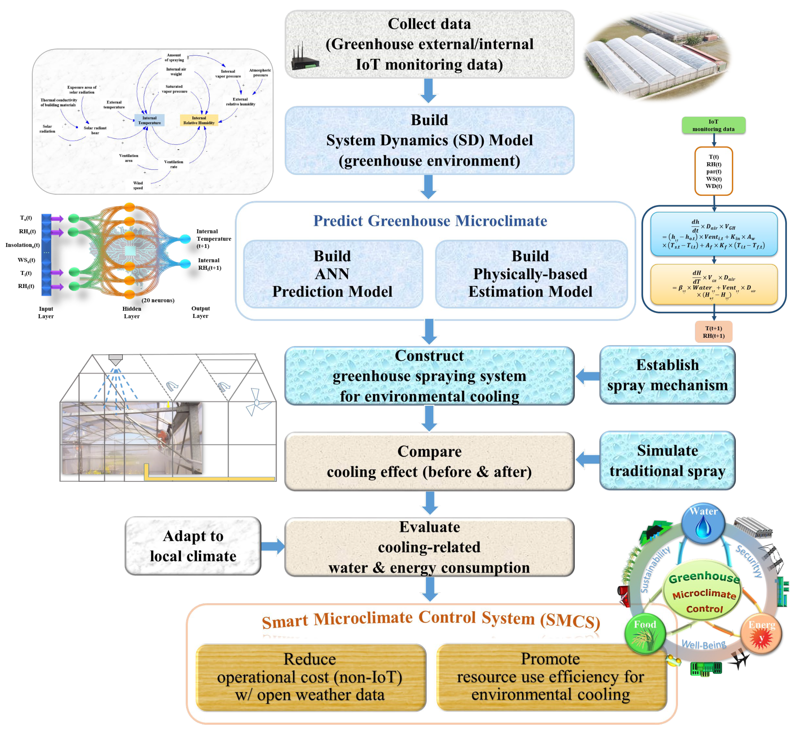
Develop a Smart Microclimate Control System for Greenhouses through System Dynamics and Machine Learning Techniques

1
Department of Bioenvironmental Systems Engineering, National Taiwan University, Taipei 10617, Taiwan
2
Taiwan Agricultural Research Institute, Taichung City 41362, Taiwan
*
Authors to whom correspondence should be addressed.
Water 2022, 14(23), 3941; https://doi.org/10.3390/w14233941
Submission received: 17 August 2022 / Revised: 29 November 2022 / Accepted: 29 November 2022 / Published: 3 December 2022

Abstract

:
Agriculture is extremely vulnerable to climate change. Greenhouse farming is recognized as a promising measure against climate change. Nevertheless, greenhouse farming frequently encounters environmental adversity, especially greenhouses built to protect against typhoons. Short-term microclimate prediction is challenging because meteorological variables are strongly interconnected and change rapidly. Therefore, this study proposes a water-centric smart microclimate-control system (SMCS) that fuses system dynamics and machine-learning techniques in consideration of the internal hydro-meteorological process to regulate the greenhouse micro-environment within the canopy for environmental cooling with improved resource-use efficiency. SMCS was assessed by in situ data collected from a tomato greenhouse in Taiwan. The results demonstrate that the proposed SMCS could save 66.8% of water and energy (electricity) used for early spraying during the entire cultivation period compared to the traditional greenhouse-spraying system based mainly on operators’ experiences. The proposed SMCS suggests a practicability niche in machine-learning-enabled greenhouse automation with improved crop productivity and resource-use efficiency. This will increase agricultural resilience to hydro-climate uncertainty and promote resource preservation, which offers a pathway towards carbon-emission mitigation and a sustainable water–energy–food nexus.

1. Introduction

The Sustainable Development Goals (SDGs) call for imperative action to ensure food security while preserving natural resources and maintaining environmental sustainability, especially in the era of climate change [1]. Significant changes in Earth’s climate have fostered more extreme weather events in recent decades and therefore have increasingly impacted global agriculture by deeply implicating the fate of food systems and directly affecting the future of “eating” for humans. For instance, Taiwan suffered from 15 extreme weather events in 2016, including 4 typhoons, 3 torrential rains, 4 severe rains, and 4 cold snaps. The huge agricultural loss caused by these extreme weather events accounted for 10.3% of the total value of agricultural production, resulting in severe fluctuations in food prices and disturbance in social equilibrium. Besides, changes in temperature and precipitation patterns may increase crop failures and production declines [2].
Agricultural systems are vulnerable to changes not only in climate but also in other evolving factors like farming practices and technology. The impacts of climate change on agricultural systems globally have been investigated in recent decades [3,4,5,6]. Greenhouses are an expensive and technological solution for the challenges climate change poses to agriculture. However, they are not a universal tool that will solve all problems since it is infeasible to grow all crops indoors. For specific, high-value crops, this makes sense. Climate-smart agriculture is an integrated approach that seeks to manage landscapes by assessing interlinked food security and climate change to simultaneously improve crop productivity as well as reduce agricultural vulnerability to pests and climate-related risks [7]. Greenhouse cultivation that creates a controllable and stable environment facilitating crop growth and yield could be a climate-smart practice [8,9,10]. Hemming et al. [11] indicated that the opportunities and challenges for the future implementation of sensor systems in greenhouses could be explored by using artificial-intelligence techniques. Greenhouse farming is recognized as a promising measure to cope with climate change because this physical practice can promote crop growth and productivity by adequately controlling a microclimate to increase food security [12,13,14]. Due to the high agricultural loss induced by extreme weather events in 2016, the Council of Agriculture in Taiwan launched a five-year funding program in December of 2016 to encourage greenhouse construction or upgrades (2000 ha expected) for mitigating agricultural losses and maintaining stable food prices in the future. Among limited managerial tools, spraying plays a pivotal role in greenhouse control of environmental cooling, especially for places like Taiwan with hot and humid weather, where environmental adversity can occur in greenhouses. For instance, Bwambale et al. [15] conducted a review of smart irrigation-monitoring and control strategies that aimed to improve water-use efficiency in precision agriculture. Tona et al. [16] conducted a technical–economic analysis on spraying equipment for specialty crops and indicated that the purchase price would make the robotic platform profitable. Spraying systems are evidently one of the key environmental-control strategies for greenhouse cultivation. Nevertheless, most of the previous research related to spraying for environmental cooling focused mainly on cooling effects [17], without considering resource consumption. For resource preservation, it is required to consider the resource-use efficiency of spraying for environmental cooling.
Greenhouse cultivation by nature substantially depends on environmental controls to stabilize crop productivity [18,19]. Accurate prediction or simulation of a greenhouse internal environment is needed to evaluate environmental-control strategies for crop growth [20,21,22,23,24,25]. Besides, short-term microclimate prediction is challenging because meteorological variables are strongly interconnected with values changing rapidly during an event. With the motivation to fill the research gap and support the above-mentioned governmental greenhouse policy to achieve SDGs #2 (Zero Hunger), #12 (Responsible Consumption and Production), and #13 (Climate Action), this study developed a water-centric smart microclimate-control system (SMCS) for greenhouse cultivation in response to climatic variation. The SMCS was designed to automatically activate early spraying for environmental cooling while consuming less water and energy. The SMCS seamlessly integrates a system-dynamics (SD) model coupled with a physically based (i.e., a hydro-meteorological process) estimation model, a machine-learning prediction model, and a spray mechanism. A traditional greenhouse-spraying system based on the physically based estimation model and the spray mechanism coupled with operators’ experience served as a benchmark for exploring the usefulness and applicability of the proposed SMCS. A tomato greenhouse located in Changhua County of Taiwan formed the case study, where the in situ datasets for use in this study were collected by Internet of Things (IoT) devices. The SMCS is expected to increase greenhouse automation and reinforce the efficiency of resource utilization, which can pave the way to reducing carbon emissions and promoting water–energy–food-nexus synergies in greenhouse farming.

2. Materials and Methods

This study proposes a water-centric SMCS that fuses system-dynamics and machine-learning techniques to regulate the greenhouse micro-environment within the canopy, with improved resource-use efficiency. The research flow chart is shown in Figure 1. We first collected the historical IoT monitoring data of the investigative greenhouse. Based on the IoT data, the SD model simulated the greenhouse microclimate within the canopy before and after spraying for environmental cooling. The back-propagation neural-network (BPNN) model predicted one-hour-ahead greenhouse internal temperature and relative humidity, where the initial inputs were the IoT data. Based on the prediction results, a spray mechanism was designed to determine the necessity of early spraying for environmental cooling. Consequently, the impacts of spraying on the internal environment and resource consumption were investigated. This study further compared the spray effects between the SMCS and the traditional greenhouse-spraying system (a benchmark), with the main focus on the resource consumption of spraying for environmental cooling. In the end, the potential of the SMCS for agricultural-loss mitigation in the perspective of water–energy–food-nexus synergies was discussed. It was noted that both traditional and machine-learning-based systems were constructed based on the IoT data collected from the same trial during 20 May and 20 July 2019.

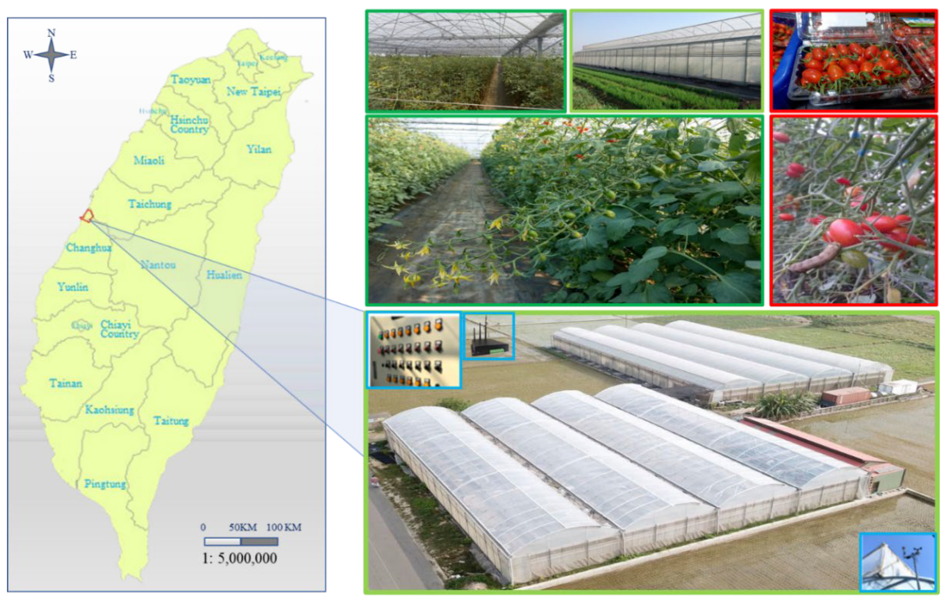
2.1. Study Area and Materials

In this study, a total of 1488 hourly meteorological datasets related to tomato cultivation were collected on 20 May and 20 July 2019 by IoT devices installed inside and outside a privately owned greenhouse located in Changhua County of Taiwan (Figure 2). The IoT devices (Figure 2) installed in the greenhouse were developed by the Taiwan Agricultural Research Institute. The size of the greenhouse is about 52 m × 30 m × 6 m (length × width × height), indicating that the land area of the greenhouse is about 1560 m2. Monitoring items consisted of internal/external temperature, internal/external relative humidity, external insolation, wind speed, and wind direction (Table 1). It is noted that this study adopted IoT datasets for model-construction and evaluation purposes only.

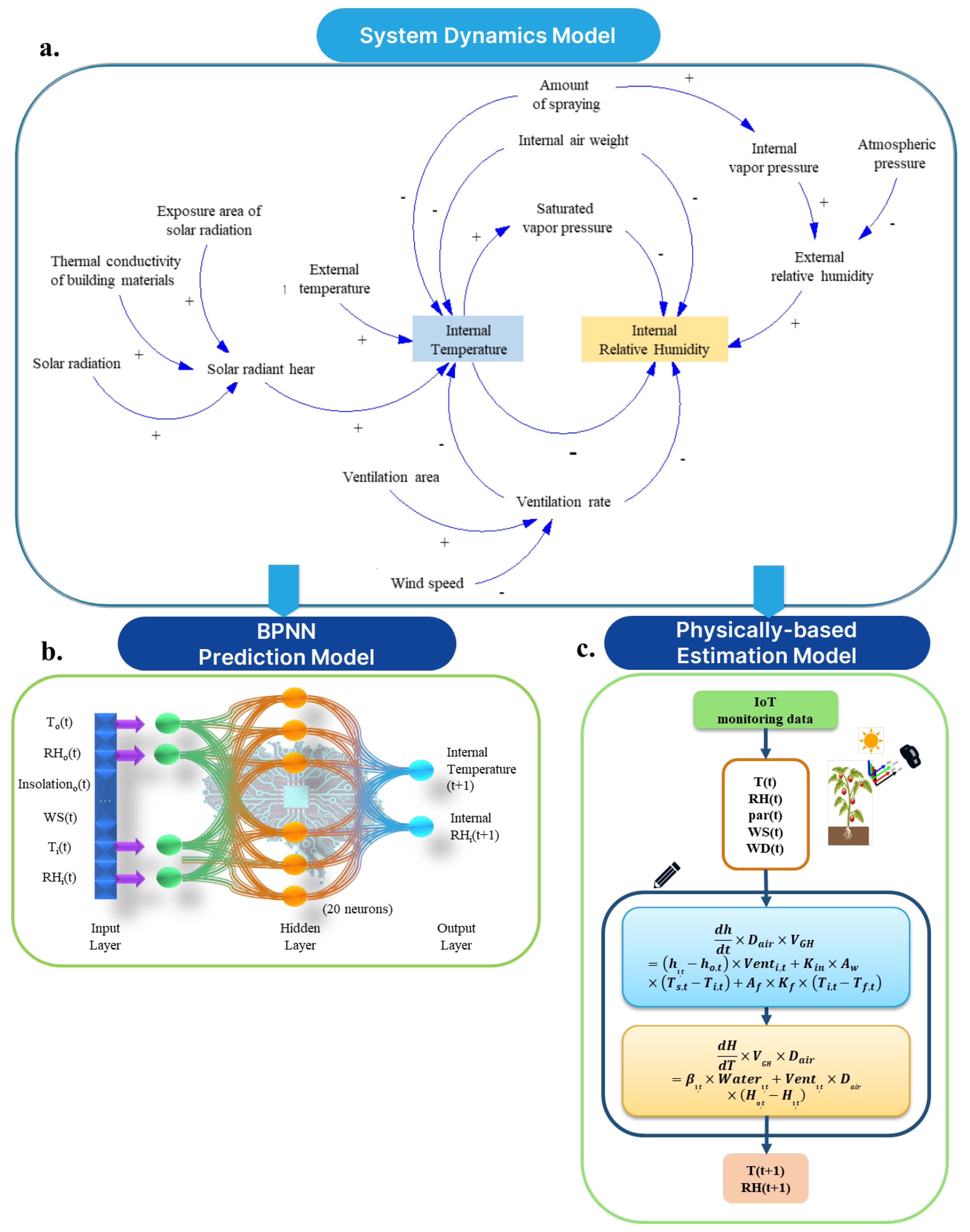
2.2. System Dynamics (SD) for Simulating Greenhouse Environment

SD is a set of process-oriented research methods specializing in the causal-feedback relationship among many variables and high-order non-linear systems [26,27,28]. It also specializes in explaining the results of system behavior through structural reasons behind the behavior [29]. SD has been widely used for simulating the non-linear behaviors in complex systems over time in various fields, including greenhouse management, forecasting and experimentation [30,31,32], rooftop farming [33], and the water–food–energy nexus [34,35].
This study explored the causal loops of SD for greenhouse cultivation by consideration the spray effect (Figure 3a). It is noted that the SMCS was constructed to reduce internal temperature and increase internal relative humidity by raising the partial pressure of water vapor to achieve the effect of cooling and humidification. A physically based model was constructed based on the SD model to estimate the greenhouse internal temperature and relative humidity before and after spraying. The framework of the SD model coupled with the physically based estimation model is shown in Figure 3.
Referring to Lee et al. [17], greenhouse internal relative humidity and temperature were considered to be a function of the conservation of mass and the conservation of energy, which consisted of two parts. Part 1 estimated the internal relative humidity by calculating enthalpy and heat conduction. Part 2 estimated the internal temperature by calculating the variation in moisture in the air. The formulation of greenhouse internal relative humidity and temperature is briefly introduced below.

2.2.1. Formulation of Greenhouse Internal Relative Humidity

The physically based estimation model of internal relative humidity was constructed by the equations of the conservation of mass and the conservation of energy (Equation (1)).
dH dt × V GH × D air = β i , t × Water i , t + Vent i , t × D air × H o , t H i , t
where dH dt is the indoor absolute humidity change rate in a time period (kg/m3 h), βi,t is the spray efficiency (%), Wateri,t denotes the amount of spray (kg), Venti,t denotes the indoor ventilation (kg/h), and Hi,t (Ho,t) denote the internal (external) absolute humidity (kg/m3) at t. VGH denotes the total capacity of the greenhouse (m3), and Dair denotes the air density (1.2 kg/m3).
H i , t = 0.62198 × RH i , t × esi i , t P atm RH i , t × esi i , t
H o , t = 0.62198 × RH o , t × esi o , t P atm RH o , t × esi o , t
where RHi,t (RHo,t) denotes the indoor (external) relative humidity (%) at t, esii,t (esio,t) denotes the indoor (external) saturated vapor pressure (kpa) at t, and Patm denotes the atmospheric pressure (101 kpa).
esi i , t = 0.6178 × e 17.2694 × T i , t T i , t + 237.3
esi o , t = 0.6178 × e 17.2694 × T o , t T o , t + 237.3
where Ti,t (To,t) denotes the indoor (external) temperature (°C) at t.
β i , t = 1.1906 0.09077 × RH i , t
Vent i , t = C i , t × WS t × A GH
where Ci,t is the ventilation utilization factor at t, AGH is the ventilation area of the greenhouse (m2), and WSt denotes the wind speed (m/h) at t.
H i , t + 1 = H i , t + dH dt
where Hi,t+1 and Hi,t denote the indoor absolute humidity at t + 1 and t (kg/m3), respectively.
ei i , t + 1 = H i , t + 1 × P atm H i , t + 1 + 0.62198
where eii,t+1 denotes the indoor partial pressure of water vapor (kpa) at t + 1.
Consequently, the internal relative humidity (RHi,t+1) at t + 1 could be calculated by Equation (10).
RH i , t + 1 = ei i , t + 1 esi i , t + 1

2.2.2. Formulation of Greenhouse Internal Temperature

The internal temperature was also constructed by the equations of the conservation of mass and the conservation of energy (Equation (11)).
dh dt × D air × V GH = h i , t h o , t × Vent i , t + K in × A w × T s , t T i , t + A f × K f × T i , t T f , t
where dh dt denotes the indoor change rate of enthalpy in a time period (kj/kg h); hi,t and ho,t denote the indoor and external enthalpies (kj/kg) in the air at t, respectively; Venti,t denotes the ventilation rate (m3/h) at t; VGH denotes the total capacity of the greenhouse (m3); Dair denotes the air density (1.2 kg/m3); Kin denotes the indoor coating material’s heat-convection parameter in the air (6.4 W/m2 °C); Aw denotes the area of the coating material (m2); Ts,t, Ti,t, and Tf,t denote the indoor temperature (°C) of the coating material, the indoor temperature (°C), and the indoor ground temperature (°C) at t, respectively; Af denotes the total ground area of the greenhouse (m2); and Kf denotes the indoor ground-to-air heat convection parameter (4.65 W/m2 °C).
h i , t = 1.006 × T i , t + H i , t × 2501 + 1.085 × T i , t
where Hi,t denotes the indoor absolute humidity (kg/m3) at t.
h o , t = 1.006 × T o , t + H o , t × 2501 + 1.085 × T o , t
where To,t denotes the external temperature (°C) at t, and Ho,t denotes the external absolute humidity (kg/m3) at t.
T s , t = T o , t + a × Rn o , t K out
where a is the solar-absorption rate on the surface of the material (0.65%), Rno,t denotes the external solar radiation (W/m2) at t, and Kout denotes the thermal conductivity on the surface of the material (6.3 W/m2 °C).
Rn o , t = 1 ref × par o , t + Rn lon
where ref denotes the ground reflectivity (0.2), paro,t denotes the external insolation at t (W/m2), and Rnlon denotes the atmospheric long-wave radiation (343 W/m2).
T f , t = T o , t + Rn o , t B × T o , t + 273.15 4 4 × B × T o , t + 273.15 3
where B is the Boltzmann constant (5.67 × 10⁻⁸ Wm−2K−4).
Because this study considered spray to be a means of humidification and cooling, it required calculating the internal heat moving away due to spray, as shown in Equation (17) (refer to [36]).
Q t = β i , t × Water i , t × H fg
where Qt denotes the heat moving away due to spray (kj/h), βi,t denotes the indoor spray efficiency (%) at t, Wateri,t denotes the indoor spray amount (kg/h) at t, and Hfg denotes the latent heat of water evaporation (2256.6 kj/kg).
dT = dh dt × V GH × D air Q t 4.186 × C p × V GH × D air
where dT denotes the indoor temperature change in a time period (°C/h), and Cp denotes the specific heat of the air (1.0052 kj/kg °C).
Consequently, the internal temperature at t + 1 could be obtained from Equation (19).
T i , t + 1 = T i , t + dT
where Ti,t+1 and Ti,t denote the indoor temperature (°C) at t + 1 and t, respectively.
Details of the formulation of greenhouse relative humidity (Part 1) and internal temperature (Part 2) can be found in the Supplementary Material.

2.3. Machine Learning for Predicting Greenhouse Internal Environment

Artificial neural networks (ANNs) in machine learning are a family of computation methods that imitate the operation and learning of the human nerve system. ANNs are broadly used to tackle diverse environmental issues, such as rainfall forecasts [37,38], evaporation prediction [39,40], flood forecasts [41,42,43,44,45,46], hydrological analysis [47,48,49,50,51], ecological-environment analysis [52,53], air-quality estimation [54], agricultural automation [55], and greenhouse environmental control [22,56,57].
The BPNN is one of the most widely used ANNs. This study utilized the BPNN to predict one-hour-ahead greenhouse internal temperature (Ti(t + 1)) and relative humidity (RHi(t + 1)) based on current information on six meteorological factors, including external temperature (To), external relative humidity (RHo), external insolation (paro) and wind speed (WS), internal temperature (Ti), and internal relative humidity (RHi) (Figure 3b). The construction of the BPNN prediction model was based on a total of 1488 hourly IoT data, where 64, 16, and 20% of the data were shuffled and randomly allocated into training, validation, and testing stages, respectively. The architecture of the BPNN model constructed in this study is illustrated in Figure 3b. The parameter setting of the BPNN model is shown in Table 2, where the number of neurons in the hidden layer and the batch size were determined to be 20 and 64, respectively, through trial-and-error processes. The relevant trial-and-error results are presented in Table 3 and Table 4.

2.4. Construction of the Spray Mechanism

Figure 4 presents the spray-simulation flow chart of the SMCS. According to the one-hour-ahead predictions (t + 1) of greenhouse internal temperature and relative humidity obtained from the BPNN model, a spray mechanism with spraying criteria was designed to determine the time to spray, which is introduced as follows.
According to Xue et al. [58] on greenhouse cultivation, the net photosynthetic rate and cumulative photosynthesis of tomato leaves could be significantly improved when the internal relative humidity reached 70%. Liou et al. [59] indicated that the formation of lycopene in tomatoes would be reduced if the greenhouse internal temperature exceeded 28 °C. Therefore, this study managed to activate sprayers for environmental cooling under two conditions: when the internal relative humidity fell below 70%, and when the internal relative humidity and the internal temperature exceeded 90% and 28 °C, respectively.
To avoid resource over-consumption, sprayers would not be activated if the internal relative humidity exceeded 90% or the internal temperature fell below 25 °C. Besides, the switching on/off of the sprayers would be carried out based on the predicted values of internal relative humidity and temperature. Therefore, the spray mechanism would activate sprayers for environmental cooling subject to two criteria: (1) the one-hour-ahead prediction of internal relative humidity would be less than 70% and the one-hour-ahead prediction of internal temperature would be higher than 25 °C, and (2) the one-hour-ahead prediction of internal relative humidity would be less than 90% and the one-hour-ahead prediction of internal temperature would be higher than 28 °C. Spraying would terminate either when the internal temperature and relative humidity met the environmental suitability for tomato growth or when the total amount of spray exceeded the maximal spray volume within one hour (i.e., 1.35 kg).
In the case of no spraying being required for environmental cooling, the one-hour-ahead predictions of internal temperature and relative humidity obtained from the BPNN model would be fed back to the system and serve as the initial input values of the BPNN model at the next time-step (the orange dotted line in Figure 4). If either above-mentioned activation criterion for spraying was met, a spray of 0.001 kg would be carried out, leading to a re-calculation of the internal temperature and relative humidity after spraying by using the physically based estimation model. The spraying process would repeat until reaching the stop criteria. It is noted that a sprayer would not be activated if the required amount of spray was less than its minimal spray volume (=the minimal duration of spray × the rate of spray). When spraying terminates, the final one-hour-ahead estimates (t + 1) of internal temperature and relative humidity obtained from the physically based model would be fed back to the system and serve as the initial input values of the BPNN model at the next time-step (the orange dotted line in Figure 4). For the greenhouse investigated and the sprayer selected for use in this study, it would require three sprayers to cover the entire greenhouse farm (1560 m2). The weight of spray each time would be 0.001 kg per sprayer, and the total weight of spray per hour would be 1.35 kg for three sprayers. Therefore, the control loop would be evaluated at a rate of 8 s.

2.5. Evaluation of Model Performances

To explore the spray effect of the SMCS on greenhouse farming, the above-mentioned spraying process for environmental cooling was implemented on all 1488 IoT data collected in this study. For comparison purposes, a traditional greenhouse-spraying system was established by integrating the physically based estimation model with the spray mechanism only, whereas the physically based model was responsible for estimating one-hour-ahead greenhouse internal temperature and relative humidity before and after spraying.
This study used the root-mean-square error (RMSE) and the coefficient of determination (R2) as the statistical indicators to evaluate model performance. Their mathematical formulas refer to Equations (20) and (21).
Root-Mean-Square Error
RMSE = 1 N i = 1 N y i o i 2
Coefficient of Determination
R 2 = i = 1 N y i y ¯ o i o ¯ i = 1 N y i y ¯ 2 i = 1 N o i o ¯ 2 2
where N is the total number of data, yi is the output value of the model, oi is the observation value, and y ¯ and o ¯ are the average of the output value and the observation value, respectively.
According to the definitions of the two indicators, it is obvious that a model is considered to perform well if it produces a higher R2 value but a lower RMSE value than the comparative model(s).

3. Results

This study developed a water-centric SMCS dedicated to greenhouse farming and the spray effect on greenhouse microclimate for environmental cooling with the relevant resource consumption being investigated. The operation of the SMCS was composed of four main phases: to simulate greenhouse environmental dynamics in consideration of the spray effect (by the SD model), to predict one-hour-ahead internal temperature and relative humidity (by the BPNN model), to determine the necessity of spraying for environmental cooling (by the spray mechanism), and to estimate the required amount of spray to manage a microclimate suitable for tomato growth in the coming hour (by the physically based model). The SMCS was applied to the 1488 in situ data collected from a greenhouse on 20 May 2019 and 20 July 2019. The modeling results are presented and discussed as follows.

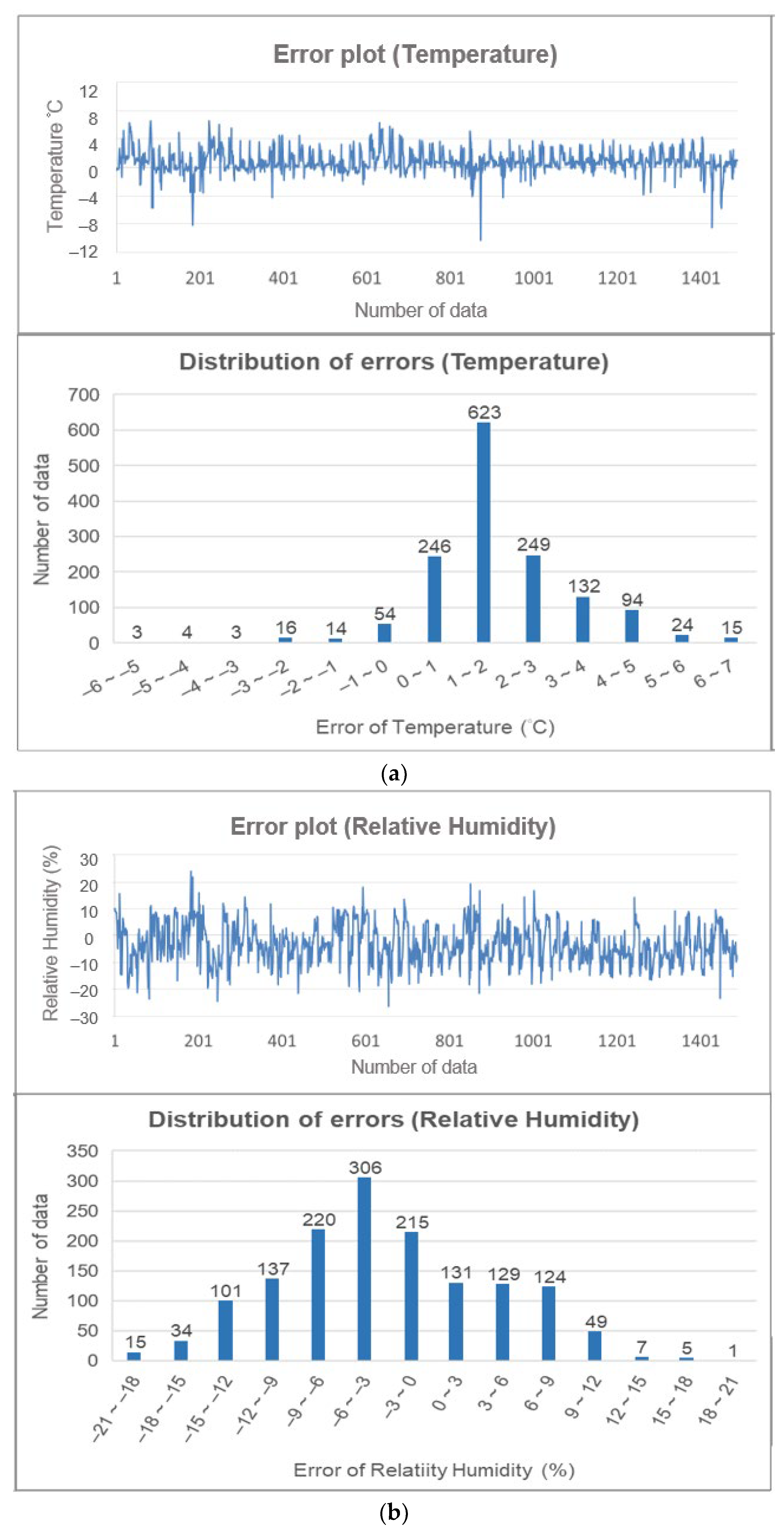
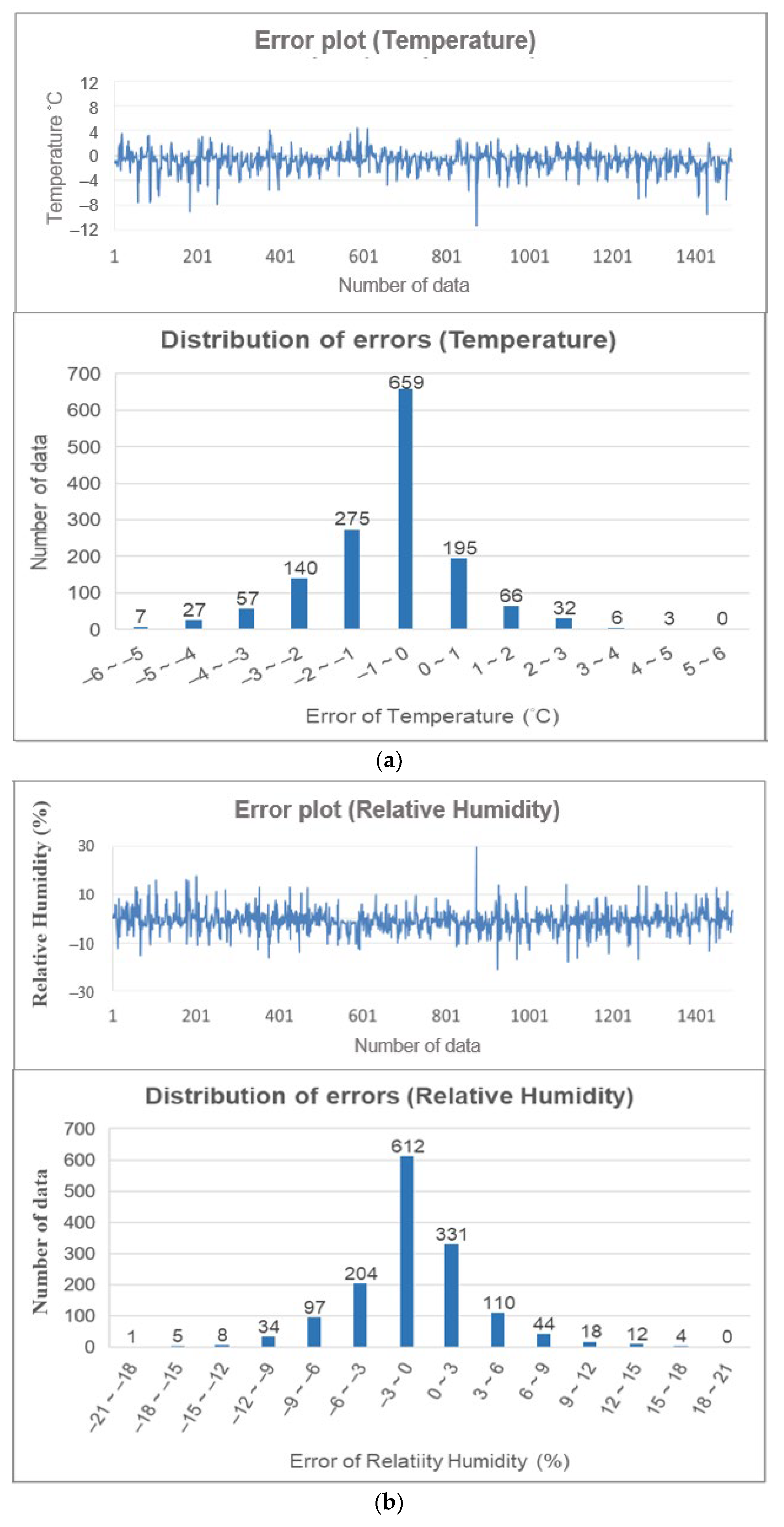
3.1. Comparison of Model Accuracy and Reliability between the Physically Based and ANN Models

Table 5 shows the performance of the physically based estimation model and the BPNN prediction model with respect to greenhouse internal temperature and relative humidity based on test datasets. For the physically based estimation model, the R2 and RMSE values of the internal temperature were 0.80 and 1.89 °C, respectively, whereas those of the internal relative humidity were 0.79 and 8.17%, respectively. The results demonstrate the accuracy and reliability of the physically based model. As for the BPNN prediction model, its R2 and RMSE values of the internal temperature were 0.83 and 1.37 °C, respectively, whereas those of the internal relative humidity were 0.88 and 3.9%, respectively. The results also demonstrate the accuracy and reliability of the BPNN model. It appears that the BPNN model is superior to the physically based model in terms of higher R2 and lower RMSE values.
Figure 5 and Figure 6 show the errors and error distributions of internal-temperature and relative-humidity estimates obtained from the physically based model and the BPNN model, respectively. In both error plots, positive values indicate overestimation whereas negative values indicate underestimation. Regarding the physically based estimation model, it can be seen in Figure 5a that the errors of the internal temperature mostly fell within 1 and 2 °C (overestimated), with an overestimation occurrence frequency (1098 times) much higher than the underestimation one (387 times). According to Figure 5b, the errors in the internal relative humidity were mostly concentrated within −3% and −6% (underestimated), with an underestimation occurrence frequency (787 times) higher than the overestimation one (699 times).
Regarding the BPNN prediction model, the results of Figure 6a indicate that the errors of the internal temperature mainly fell within −1 and 0 °C (under prediction), where underprediction (1176 times) occurred more frequently than overprediction (302 times). According to Figure 6b, the errors in the internal relative humidity were mainly concentrated within −3% and 0%, where underprediction (959 times) also occurred more frequently than overprediction (517 times). It also appears that the BPNN model performed better than the physically based model in terms of smaller error ranges and error distributions centering at zero.
Furthermore, the results shown in Table 5 and Figure 5 and Figure 6 are quite consistent, which shows that the overall performance of the BPNN model was slightly better than that of the physically based model. This recommended the incorporation of the BPNN model into the SMCS to predict one-hour-ahead internal temperature and relative humidity in this study.

3.2. Comparison of the Spray Effect of Traditional and Smart Control Systems on Greenhouse Internal Environment

Table 6 and Table 7 show the results of internal temperature and relative humidity before and after spraying by the traditional spraying system and the proposed SMCS, respectively.
The results of Table 6 indicate that the average and standard deviation of the internal temperature after spraying decreased by 2.6 and 2.3 °C, respectively. For the internal relative humidity after spraying, the average value increased from 72% to 86%, whereas the standard deviation dropped from 16% to 7%.
The results of Table 7 show that both the average and standard deviation of the internal temperature after spraying decreased by 1.4 °C. For the internal relative humidity after spraying, the average value increased from 74% to 89%, whereas the standard deviation dropped from 12% to 4%. These results demonstrate that the SMCS could more effectively reduce the internal temperature while increasing the internal relative humidity after spraying than the traditional one, which supports the practicability of the proposed SMCS on greenhouse farms.

3.3. Comparison of Resource Consumption between Traditional and Smart Microclimate-Control Systems

Concerning spray-related resources utilization for greenhouse environmental control over the entire investigative period, water consumption could be obtained directly from summing up the amount of spray at each time-step while power consumption would be converted from horsepower and the total operating hours of the sprayers. For spray-simulation purposes, this study adopted the “FH-09 power spray motor” sprayer launched by the Fog Century Environmental Protection and Energy Saving Enterprise Co. Ltd., located in Taichung City, Taiwan. The main specifications of the sprayer are a horsepower of 1.125 kW, a water absorption of 0.15 kg/h, and an applicable area of about 400 to 600 m2. Considering the greenhouse investigated in this study occupies an area of 1560 m2, it would require three sprayers to cover the entire greenhouse farm.
Table 8 compares the traditional and the proposed control systems regarding the resource consumption of spraying for environmental cooling.
It is noted that the numbers of the on/off switches of the sprayers associated with the two comparative systems differed slightly (736 times for the traditional system vs. 726 times for the smart system). Therefore, the difference of the two systems in power consumption enabling the switching on/off of the sprayers could be ignored. Under this assumption, the traditional system consumed about 129,478 kg of water and 90 kWh of electric power for greenhouse environmental control during the entire tomato-cultivation period. In contrast, the SMCS only consumed about 42,962 kg of water and 29.8 kWh of electric power. The results demonstrate that the SMCS consumed far fewer resources for spraying than the traditional system, with water- and power-saving rates reaching 66.8%. It was further noticed that early spraying for environmental cooling suggested by the SMCS allowed the wind to blow away excess internal water vapor one hour ahead, leading to a decrease in the internal relative humidity. Spray efficiency is known to be inversely proportional to the internal relative humidity. Therefore, the amount of spray could be reduced due to early spraying.

4. Discussion

4.1. Evaluation of Hazard Mitigation by the SMCS

This study further evaluated the potential contribution of the proposed SMCS to the governmental greenhouse policy launched in 2016 regarding the construction of 2000 ha of reinforced greenhouses within five years. Taking the agricultural loss in 2020 released by the Council of Agriculture in Taiwan as an example, under the scenario that all 2000 ha of greenhouses could be equipped with the SMCS, the agricultural loss caused by extreme weather events would be significantly reduced by 22% (=2000 (greenhouse area in ha)/9097 (total damaged area in ha)) on average. Besides, resource saving in water and energy would achieve 1,109,918 tons (=((86,516 kg/1560 m2) × 10,000) × 2000 ha/1000) and 771,795 kWh (=((60.2 kWh/1560 m2) × 10,000) × 2000 ha), respectively (Table 8). This suggests the smart greenhouse microclimate-control practice bears high potential for tackling climate change and can significantly promote the nexus synergies among water, energy, and food, especially when encountering extreme weather events.

4.2. Conributions of the SMCS

The proposed SMCS makes two main contributions. Firstly, for maintaining an environment suitable for crop growth, the traditional greenhouse-spraying system requires monitoring sensors like IoT devices to detect the internal temperature or relative humidity for switching sprayers on/off. Nevertheless, this may impose the risk of an unsuitable environment on greenhouse farming between two time-steps. For example, the operational time interval was one hour in this study. Even if the greenhouse environment complies with the suitability conditions of crop growth at the current minute, it may violate the suitability conditions in the next minute. In contrast, the SMCS can predict the greenhouse microclimate for the next hour well, thereby spraying in advance to prevent an unsuitable environment for crop growth. Besides, the SMCS avoids using IoT sensors because the extra hardware and maintenance costs of the monitoring devices also place a heavy burden on greenhouse owners. Secondly, the SMCS consumes fewer resources of water and energy (electricity) when spraying for environmental cooling than the traditional method, indicating that the SMCS can mitigate greenhouse-gas emissions. Low resource consumption also represents cost-effectiveness and relatively high profits, leading to more commercial value that can be achieved by the SMCS.
The greenhouse-management practice developed can be applied to crops and areas of interest with adequate modification of the environmental suitability for crop growth. Similar methodology for developing the SMCS can also be applied to different greenhouse types. Future research can consider incorporating crop evapotranspiration, soil-moisture content, nutrients, and fertilization into the SMCS to increase the prediction accuracy of the greenhouse environment and promote crop productivity and quality. Ventilation is also a major factor in the control of greenhouse temperature. In future research, ventilation will be considered by incorporating the greenhouse-control factors (e.g., skylight, roller shades on each wall, and inner shade net) into the proposed water-centric smart microclimate-control system (SMCS) to increase its operational efficiency and effectiveness.

5. Conclusions

This study proposed a water-centric smart microclimate-control system (SMCS) for greenhouse farming, with a mission to manage the microclimate through efficient spraying for environmental cooling. The SMCS can maintain stable crop productivity when extreme weather events occur. The SMCS can determine the necessity of spraying for environmental cooling according to the predictions of greenhouse internal temperature and relative humidity. The results demonstrate that the SMCS could achieve the same environmental-control effect as the traditional one while consuming far fewer resources for spraying, which makes greenhouse farming move towards carbon-emission mitigation and sustainable management of the water–energy–food nexus. There are four main findings drawn from this study, shown below.
Firstly, the cost of sensor installation is a major concern for farmers in Taiwan, especially concerning device investment and maintenance issues. The BPNN model could (Figure 1) predict greenhouse microclimate based on external climate conditions with less water and energy. After the BPNN model is constructed, this science-based management practice requires no in situ monitoring sensors, which favorably lessens greenhouse owners’ investment in environmental control and makes a positive contribution to the overall cost–benefit ratio of greenhouse farming. The physically based model engaging the internal hydro-meteorological process could produce satisfactory accuracy and reliability in estimating greenhouse microclimate, despite it performing slightly worse than the BPNN prediction model.
Secondly, the SMCS could predict the greenhouse internal environment well one hour ahead and spray in advance when needed for environmental cooling, which prevents crops from being exposed to an unsuitable cultivation environment.
Thirdly, the SMCS could achieve savings as high as 66.8% of water and energy compared to the traditional method. Therefore, the SMCS gains more commercial value than the traditional method because low resource consumption means low production cost and relatively high profits.
Fourthly, the reduction in agricultural loss caused by extreme weather events in 2020 would reach 22% if the SMCS could be implemented in 2000 ha of greenhouses (the goal of the governmental greenhouse policy launched in 2016 in Taiwan). This would lead to effective resource saving in water and energy of 1,109,918 tons and 771,795 kWh per year, respectively. This greenhouse-control strategy significantly contributes to environmental sustainability and greenhouse-gas-emission mitigation.
This study suggests a practicability niche in machine-learning-enabled greenhouse automation with improved crop productivity and resource-use efficiency. The proposed SMCS substantially moves greenhouse farming towards the SDGs in the perspectives of food security, natural-resource preservation, and environmental sustainability.

Supplementary Materials

The following supporting information can be downloaded at: https://www.mdpi.com/article/10.3390/w14233941/s1, Formulation of the physically based estimation model.

Author Contributions

Conceptualization, T.-H.C. and F.-J.C.; methodology, T.-H.C. and C.-H.H.; software, T.-H.C. and C.-H.H.; validation, M.-H.L., I.-W.H. and M.-H.Y.; formal analysis, T.-H.C. and C.-H.H.; investigation, M.-H.L. and I.-W.H.; resources, M.-H.Y. and F.-J.C.; data curation, T.-H.C. and M.-H.Y.; writing—original draft preparation, T.-H.C.; writing—review and editing, F.-J.C.; visualization, T.-H.C., M.-H.L. and I.-W.H.; supervision, F.-J.C.; project administration, F.-J.C.; funding acquisition, F.-J.C. and M.-H.Y. All authors have read and agreed to the published version of the manuscript.

Funding

This research was funded by the National Science and Technology Council, Taiwan, grant numbers 110-2313-B-002-034-MY3 and 110-2321-B-055-001-.

Data Availability Statement

The data presented in this study are available on request from the corresponding author.

Acknowledgments

The datasets provided by the Central Weather Bureau in Taiwan and the Taiwan Agricultural Research Institute are acknowledged. The authors would like to thank the editors and anonymous reviewers for their constructive comments that greatly enriched the manuscript.

Conflicts of Interest

The authors declare no conflict of interest.

References

  1. United Nations. The Sustainable Development Goals Report 2022; United Nations Publications: New York, NY, USA, 2022; pp. 6–25. [Google Scholar]
  2. Huang, A.; Chang, F.J. Using a self-organizing map to explore local weather features for smart urban agriculture in northern Taiwan. Water 2021, 13, 3457. [Google Scholar] [CrossRef]
  3. Walters, S.A.; Gajewski, C.; Sadeghpour, A.; Groninger, J.W. Mitigation of climate change for urban agriculture: Water management of culinary herbs grown in an extensive green roof environment. Climate 2022, 10, 180. [Google Scholar] [CrossRef]
  4. Holzkämper, A. Adapting agricultural production systems to climate change—What’s the use of models? Agriculture 2017, 7, 86. [Google Scholar] [CrossRef] [Green Version]
  5. Salpina, D.; Pagliacci, F. Are we adapting to climate change? Evidence from the high-quality agri-food sector in the Veneto region. Sustainability 2022, 14, 11482. [Google Scholar] [CrossRef]
  6. Shayanmehr, S.; Porhajašová, J.I.; Babošová, M.; Sabouhi Sabouni, M.; Mohammadi, H.; Rastegari Henneberry, S.; Shahnoushi Foroushani, N. The impacts of climate change on water resources and crop production in an arid region. Agriculture 2022, 12, 1056. [Google Scholar] [CrossRef]
  7. Xin, Y.; Tao, F. Developing climate-smart agricultural systems in the North China Plain. Agric. Ecosyst. Environ. 2020, 291, 106791. [Google Scholar] [CrossRef]
  8. Esmaili, M.; Aliniaeifard, S.; Mashal, M.; Vakilian, K.A.; Ghorbanzadeh, P.; Azadegan, B.; Seif, M.; Didaran, F. Assessment of adaptive neuro-fuzzy inference system (ANFIS) to predict production and water productivity of lettuce in response to different light intensities and CO2 concentrations. Agric. Water Manag. 2021, 258, 107201. [Google Scholar] [CrossRef]
  9. Kalkhajeh, Y.K.; Huang, B.; Hu, W.; Ma, C.; Gao, H.; Thompson, M.L.; Hansen, H.C.B. Environmental soil quality and vegetable safety under current greenhouse vegetable production management in China. Agric. Ecosyst. Environ. 2021, 307, 107230. [Google Scholar] [CrossRef]
  10. Li, M.; Chen, S.; Liu, F.; Zhao, L.; Xue, Q.; Wang, H.; Chen, M.; Lei, P.; Wen, D.; Sanchez-Molina, J.A.; et al. A risk management system for meteorological disasters of solar greenhouse vegetables. Precis. Agric. 2017, 18, 997–1010. [Google Scholar] [CrossRef]
  11. Hemming, S.; Zwart, F.D.; Elings, A.; Petropoulou, A.; Righini, I. Cherry tomato production in intelligent greenhouses—Sensors and AI for control of climate, irrigation, crop yield, and quality. Sensors 2020, 20, 6430. [Google Scholar] [CrossRef]
  12. Huang, Y.I. Study of fog and fan system for plastic greenhouse cooling in Taiwan. J. Agric. Mach. 1999, 8, 17–27. [Google Scholar]
  13. Joudi, K.A.; Farhan, A.A. A dynamic model and an experimental study for the internal air and soil temperatures in an innovative greenhouse. Energy Convers. Manag. 2015, 91, 76–82. [Google Scholar] [CrossRef]
  14. Pawlowski, A.; Sánchez-Molina, J.A.; Guzmán, J.L.; Rodríguez, F.; Dormido, S. Evaluation of event-based irrigation system control scheme for tomato crops in greenhouses. Agric. Water Manag. 2017, 183, 16–25. [Google Scholar] [CrossRef]
  15. Bwambale, E.; Abagale, F.K.; Anornu, G.J. Smart irrigation monitoring and control strategies for improving water use efficiency in precision agriculture: A review. Agric. Water Manag. 2022, 260, 107324. [Google Scholar] [CrossRef]
  16. Tona, E.; Calcante, A.; Oberti, R. The profitability of precision spraying on specialty crops: A technical–economic analysis of protection equipment at increasing technological levels. Precis. Agric. 2018, 19, 606–629. [Google Scholar] [CrossRef] [Green Version]
  17. Lee, S.C.; Chang, C.Y.; Lee, W.S. The Study on Greenhouse Cooling Effect on Different Control Strategies for Fogging System. J. Agric. Mach. 2006, 15, 23–36. [Google Scholar]
  18. Chen, S.; Cai, L.; Zhang, H.; Zhang, Q.; Song, J.; Zhang, Z.; Deng, Y.; Liu, Y.; Wang, X.; Fang, H. Deposition distribution, metabolism characteristics, and reduced application dose of difenoconazole in the open field and greenhouse pepper ecosystem. Agric. Ecosyst. Environ. 2021, 313, 107370. [Google Scholar] [CrossRef]
  19. Hu, J.; Gettel, G.; Fan, Z.; Lv, H.; Zhao, Y.; Yu, Y.; Wang, J.; Butterbach-Bahl, K.; Li, G.; Lin, S. Drip fertigation promotes water and nitrogen use efficiency and yield stability through improved root growth for tomatoes in plastic greenhouse production. Agric. Ecosyst. Environ. 2021, 313, 107379. [Google Scholar] [CrossRef]
  20. Ding, J.T.; Tu, H.Y.; Zang, Z.L.; Huang, M.; Zhou, S.J. Precise control and prediction of the greenhouse growth environment of Dendrobium candidum. Comput. Electron. Agric. 2018, 151, 453–459. [Google Scholar] [CrossRef]
  21. Hamrani, A.; Akbarzadeh, A.; Madramootoo, C.A. Machine learning for predicting greenhouse gas emissions from agricultural soils. Sci. Total Environ. 2020, 741, 140338. [Google Scholar] [CrossRef]
  22. Jung, D.H.; Kim, H.S.; Jhin, C.; Kim, H.J.; Park, S.H. Time-serial analysis of deep neural network models for prediction of climatic conditions inside a greenhouse. Comput. Electron. Agric. 2020, 173, 105402. [Google Scholar] [CrossRef]
  23. Katzin, D.; van Henten, E.J.; van Mourik, S. Process-based greenhouse climate models: Genealogy, current status, and future directions. Agric. Syst. 2022, 198, 103388. [Google Scholar] [CrossRef]
  24. Rincón, V.J.; Grella, M.; Marucco, P.; Alcatrão0, A.E.; Sanchez-Hermosilla, J.; Balsari, P. Spray performance assessment of a remote-controlled vehicle prototype for pesticide application in greenhouse tomato crops. Sci. Total Environ. 2020, 726, 138509. [Google Scholar] [CrossRef] [PubMed]
  25. Rodriguez-Ortega, W.M.; Martinez, V.; Rivero, R.M.; Camara-Zapata, J.M.; Mestre, T.; Garcia-Sanchez, F. Use of a smart irrigation system to study the effects of irrigation management on the agronomic and physiological responses of tomato plants grown under different temperatures regimes. Agric. Water Manag. 2017, 183, 158–168. [Google Scholar] [CrossRef]
  26. Astegiano, P.; Fermi, F.; Martino, A. Investigating the impact of e-bikes on modal share and greenhouse emissions: A system dynamic approach. Transp. Res. Procedia 2019, 37, 163–170. [Google Scholar] [CrossRef]
  27. Forrester, J.W. System dynamics and the lessons of 35 years. In A Systems-Based Approach to Policymaking; Springer: Boston, MA, USA, 1993; pp. 199–240. [Google Scholar]
  28. Li, J.W.; Cao, Y.C.; Zhu, Y.Q.; Xu, C.; Wang, L.X. System dynamic analysis of greenhouse effect based on carbon cycle and prediction of carbon emissions. Appl. Ecol. Environ. Res. 2019, 17, 5067–5080. [Google Scholar] [CrossRef]
  29. Forrester, J.W. Industrial dynamics. J. Oper. Res. Soc. 1997, 48, 1037–1041. [Google Scholar] [CrossRef]
  30. Château, P.A.; Wunderlich, R.F.; Wang, T.W.; Lai, H.T.; Chen, C.C.; Chang, F.J. Mathematical modeling suggests high potential for the deployment of floating photovoltaic on fish ponds. Sci. Total Environ. 2019, 687, 654–666. [Google Scholar] [CrossRef] [PubMed]
  31. Lu, D.; Iqbal, A.; Zan, F.; Liu, X.; Chen, G. Life-cycle-based rgeenhouse gas, energy, and economic analysis of municipal solid wastemanagement using system dynamics model. Sustainability 2021, 13, 1641. [Google Scholar] [CrossRef]
  32. Stasinopoulos, P.; Shiwakoti, N.; Beining, M. Use-stage life cycle greenhouse gas emissions of the transition to an autonomous vehicle fleet: A system dynamics approach. J. Clean. Prod. 2021, 278, 123447. [Google Scholar] [CrossRef]
  33. Huang, A.; Chang, F.J. Prospects for rooftop farming system dynamics: An action to stimulate water-energy-food nexus synergies toward green cities of tomorrow. Sustainability 2021, 13, 9042. [Google Scholar] [CrossRef]
  34. Amadei, B. A Systems Approach to Modeling the Water-Energy-Land-Food Nexus: System Dynamics MODELING and dynamic Scenario Planning, 1st ed.; Momentum Press: New York, NY, USA, 2019; Volume I, II. [Google Scholar]
  35. Gary, I.E.; Grigg, N.; Reagan, W. Dynamic behavior of the water-food-energy nexus: Focus on crop production and consumption. Irrig. Drain. 2017, 66, 19–33. [Google Scholar]
  36. Fang, W. Quantitative measures of the effectiveness of evaporative cooling systems in greenhouse. J. Agric. Mach. 1995, 4, 15–25. [Google Scholar]
  37. Chang, F.J.; Tsai, M.J. A nonlinear spatio-temporal lumping of radar rainfall for modeling multi-step-ahead inflow forecasts by data-driven techniques. J. Hydrol. 2016, 535, 256–269. [Google Scholar] [CrossRef]
  38. Mirabbasi, R.; Kisi, O.; Sanikhani, H.; Gajbhiye Meshram, S. Monthly long-term rainfall estimation in Central India using M5Tree, MARS, LSSVR, ANN and GEP models. Neural Comput. Appl. 2019, 31, 6843–6862. [Google Scholar] [CrossRef]
  39. Arya Azar, N.; Kardan, N.; Ghordoyee Milan, S. Developing the artificial neural network–evolutionary algorithms hybrid models (ANN–EA) to predict the daily evaporation from dam reservoirs. Eng. Comput. 2021, 37, 1–19. [Google Scholar] [CrossRef]
  40. Chang, F.J.; Chang, L.C.; Kao, H.S.; Wu, G.R. Assessing the effort of meteorological variables for evaporation estimation by self-organizing map neural network. J. Hydrol. 2010, 384, 118–129. [Google Scholar] [CrossRef]
  41. Chang, L.C.; Amin, M.; Yang, S.N.; Chang, F.J. Building ANN-based regional multi-step-ahead flood inundation forecast models. Water 2018, 10, 1283. [Google Scholar] [CrossRef] [Green Version]
  42. Chang, L.C.; Chang, F.J.; Yang, S.N.; Tsai, F.H.; Chang, T.H.; Herricks, E.E. Self-organizing maps of typhoon tracks allow for flood forecasts up to two days in advance. Nat. Commun. 2020, 11, 1–13. [Google Scholar] [CrossRef] [Green Version]
  43. Chang, L.C.; Liou, C.Y.; Chang, F.J. Explore training self-organizing map methods for clustering high-dimensional flood inundation maps. J. Hydrol. 2022, 595, 125655. [Google Scholar] [CrossRef]
  44. Kao, I.F.; Zhou, Y.; Chang, L.C.; Chang, F.J. Exploring a long short-term memory based encoder-decoder framework for multi-step-ahead flood forecasting. J. Hydrol. 2020, 583, 124631. [Google Scholar] [CrossRef]
  45. Zhou, Y.; Chang, L.C.; Uen, T.S.; Guo, S.; Xu, C.Y.; Chang, F.J. Prospect for small-hydropower installation settled upon optimal water allocation: An action to stimulate synergies of water-food-energy nexus. Appl. Energy 2019, 238, 668–682. [Google Scholar] [CrossRef]
  46. Zhou, Y.; Guo, S.; Xu, C.Y.; Chang, F.J.; Yin, J. Improving the reliability of probabilistic multi-step-ahead flood forecasting by fusing unscented Kalman filter with recurrent neural network. Water 2020, 12, 578. [Google Scholar] [CrossRef] [Green Version]
  47. Chang, F.J.; Guo, S. Advances in hydrologic forecasts and water resources management. Water 2020, 12, 1819. [Google Scholar] [CrossRef]
  48. Bai, T.; Tsai, W.P.; Chiang, Y.M.; Chang, F.J.; Chang, W.Y.; Chang, L.C.; Chang, K.C. Modeling and investigating the mechanisms of groundwater level variation in the Jhuoshui River Basin of Central Taiwan. Water 2019, 11, 1554. [Google Scholar] [CrossRef] [Green Version]
  49. Chen, I.T.; Chang, L.C.; Chang, F.J. Exploring the spatio-temporal interrelation between groundwater and surface water by using the self-organizing maps. J. Hydrol. 2018, 556, 131–142. [Google Scholar] [CrossRef]
  50. Ghimire, S.; Deo, R.C.; Downs, N.J.; Raj, N. Global solar radiation prediction by ANN integrated with European Centre for medium range weather forecast fields in solar rich cities of Queensland Australia. J. Clean. Prod. 2019, 216, 288–310. [Google Scholar] [CrossRef]
  51. Pradhan, P.; Tingsanchali, T.; Shrestha, S. Evaluation of soil and water assessment tool and artificial neural network models for hydrologic simulation in different climatic regions of Asia. Sci. Total Environ. 2020, 701, 134308. [Google Scholar] [CrossRef]
  52. Cheng, S.T.; Tsai, W.P.; Yu, T.C.; Herricks, E.E.; Chang, F.J. Signals of stream fish homogenization revealed by AI-based clusters. Sci. Rep. 2018, 8, 15960. [Google Scholar] [CrossRef] [Green Version]
  53. Hu, J.H.; Tsai, W.P.; Cheng, S.T.; Chang, F.J. Explore the relationship between fish community and environmental factors by machine learning techniques. Environ. Res. 2020, 184, 109262. [Google Scholar] [CrossRef]
  54. Kow, P.Y.; Wang, Y.S.; Zhou, Y.; Kao, I.F.; Issermann, M.; Chang, L.C.; Chang, F.J. Seamless integration of convolutional and back-propagation neural networks for regional multi-step-ahead PM2.5 forecasting. J. Clean. Prod. 2020, 261, 121285. [Google Scholar] [CrossRef]
  55. Saleem, M.H.; Potgieter, J.; Arif, K.M. Automation in agriculture by machine and deep learning techniques: A review of recent developments. Precis. Agric. 2021, 22, 2053–2091. [Google Scholar] [CrossRef]
  56. Nicolosi, G.; Volpe, R.; Messineo, A. An innovative adaptive control system to regulate microclimatic conditions in a greenhouse. Energies 2017, 10, 722. [Google Scholar] [CrossRef] [Green Version]
  57. Riahi, J.; Vergura, S.; Mezghani, D.; Mami, A. Intelligent control of the microclimate of an agricultural greenhouse powered by a supporting PV system. Appl. Sci. 2020, 10, 1350. [Google Scholar] [CrossRef]
  58. Xue, Y.X.; Li, Y.L.; Wen, X.Z. Effects of air humidity on the photosynthesis and fruit-set of yomato under high Temperature. Acta Hortic. Sin. 2010, 37, 397–404. [Google Scholar]
  59. Liou, Y.C.; Huang, R.J.; Cai, M.L.; Huang, S.W. Facility cultivation and health management techniques of grape tomato. Tech. Issue Tainan Dist. Agric. Res. Ext. Stn. 2016, 164, 3–47. (In Chinese) [Google Scholar]
Figure 1. Research flow chart of this study.
Water 14 03941 g001
Figure 2. Location and structure of the greenhouse investigated in this study.
Water 14 03941 g002
Figure 3. Model construction of the proposed smart microclimate-control system (SMCS) for greenhouse cultivation in consideration of the spray effect. (a). SD model. (b). BPNN prediction model. (c). Physically based estimation model.
Water 14 03941 g003
Figure 4. Spray-simulation flow chart of the SMCS that integrates the SD model, the BPNN prediction model, the physically based estimation model, and the spray mechanism.
Water 14 03941 g004
Figure 5. Errors and error distributions of greenhouse microclimate estimates from the physically based model (20 May 2019–20 July 2019). (a). Internal temperature. (b). Internal relative humidity.
Water 14 03941 g005
Figure 6. Errors and error distributions of greenhouse microclimate predictions from the BPNN model (20 May 2019–20 July 2019). (a). Internal temperature. (b). Internal relative humidity.
Water 14 03941 g006
Table 1. IoT monitoring data collected in this study for model-validation purposes (20 May–20 July 2019 at a 10 min scale).
ItemNotationSI Unit
External temperatureTo°C
External relative humidityRHo%
External insolationparoW/m2
Wind speedWSm/s
Wind directionWD°
Internal temperatureTi°C
Internal relative humidityRHi%
Table 2. Parameter setting of the BPNN model.
ItemBPNN
Number of hidden neurons10, 20, 40
Number of epochs200
Early stopping20
Batch size8, 16, 32, 64
Learning rate0.001
Activation functionScaled exponential linear unit (SELU)
OptimizerAdam
Table 3. Trial-and-error results of the number of hidden neurons in the BPNN model.
Number of Hidden NeuronsTemperatureRelative Humidity
R2RMSER2RMSE
100.801.61 °C0.874.45%
20 10.821.55 °C0.884.19%
400.812.42 °C0.874.40%
Note: 1 The number of hidden neurons that was determined for constructing the BPNN model in consideration of the model complexity and the values of the evaluation indicators.
Table 4. Trial-and-error results of the batch number in the BPNN model.
Batch NumberTemperatureRelative Humidity
R2RMSER2RMSE
80.832.08 °C0.884.28%
160.811.56 °C0.874.53%
320.821.67 °C0.884.35%
64 10.831.55 °C0.884.19%
Note: 1 The batch number that was determined for constructing the BPNN model in consideration of the values of the evaluation indicators.
Table 5. Performance of the physically based estimation model and the BPNN prediction model with respect to greenhouse internal temperature and relative humidity based on test datasets.
IndicatorsTemperatureRelative Humidity
Physically BasedBPNNPhysically BasedBPNN
R20.800.830.790.88
RMSE1.89 °C1.37 °C8.17%3.9%
Table 6. Results of greenhouse environmental control on internal temperature and relative humidity before and after spraying for environmental cooling by the traditional spraying system (20 May 2019–20 July 2019).
IndicatorsTemperatureRelative Humidity
BeforeAfterBeforeAfter
Max38.8 °C28.1 °C100%100%
Min23.8 °C23.8 °C37%56%
Average29.6 °C27.0 °C72%86%
Standard deviation3.6 °C1.3 °C16%7%
Table 7. Results of greenhouse environmental control on internal temperature and relative humidity before and after spraying for environmental cooling by the SMCS (20 May 2019–20 July 2019).
IndicatorsTemperatureRelative Humidity
BeforeAfterBeforeAfter
Max34.3 °C32.9 °C91%100%
Min21.3 °C22.1 °C48%69%
Average28.0 °C26.6 °C74%89%
Standard deviation2.9 °C1.5 °C12%4%
Table 8. Comparison between traditional and smart microclimate-control systems regarding the resource consumption of spraying for environmental cooling.
ItemWater
(kg)
Electric Power
(kWh)
Number of On/Off Switch of Sprayers
Traditional spraying system129,47890.0736/1488
Smart spraying system42,96229.8726/1488
Resource-saving amount 186,51660.210/-
Resource-saving rate 266.8%66.8%1.4%/-
Traditional spraying system129,47890.0736/1488
Notes: 1 Amount of the traditional spraying system—amount of the SMCS. 2 Resource saving amount/amount of the traditional spraying system.
Publisher’s Note: MDPI stays neutral with regard to jurisdictional claims in published maps and institutional affiliations.

