Comparison of Rain Gauge Network and Weather Radar Data: Case Study in Angra dos Reis, Brazil

 ,
, 
 ,
,  and
and 
Abstract
:1. Introduction
2. Materials and Methods
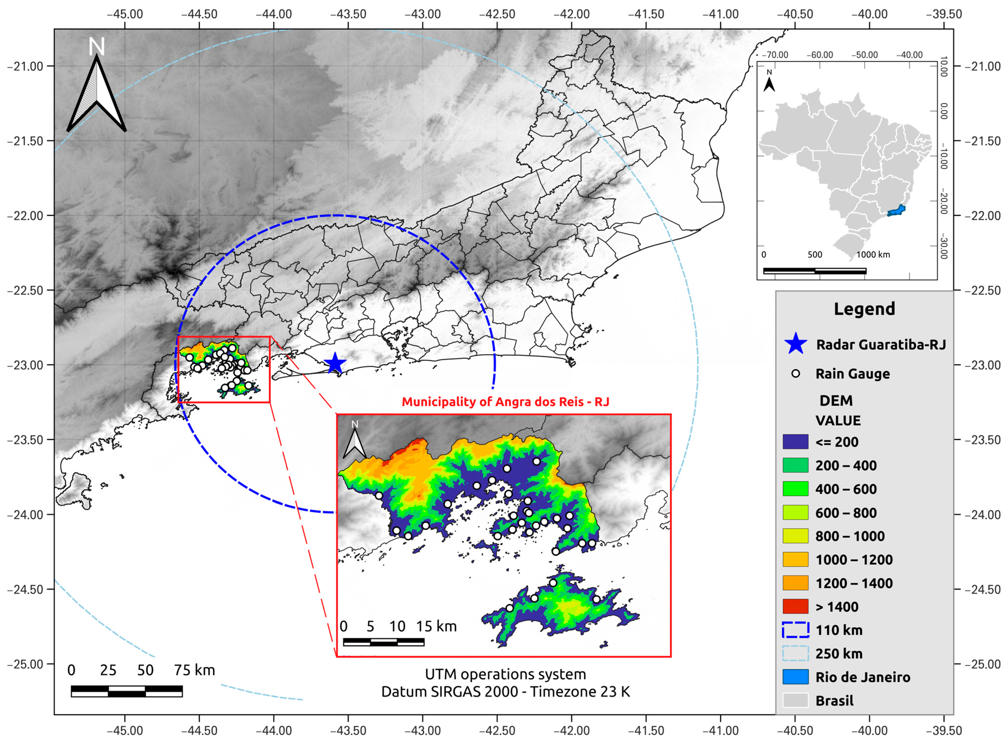
2.1. Case Study Area
2.2. Rainfall Data
2.2.1. Rain Gauge Data
2.2.2. Radar Data
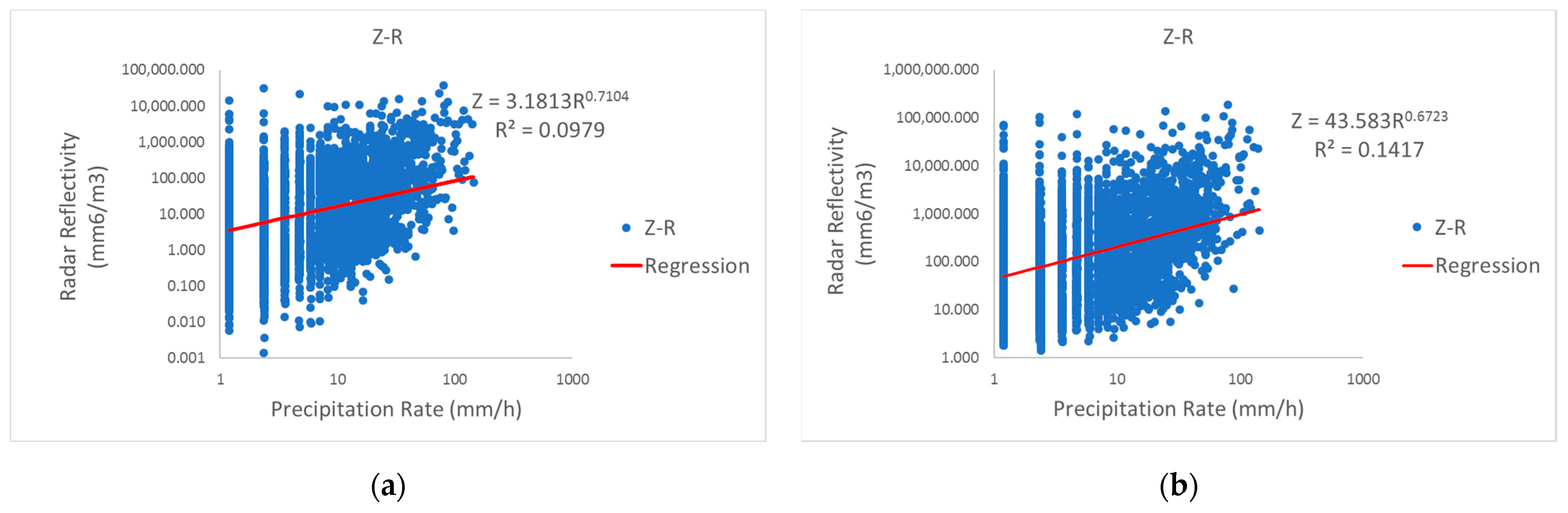
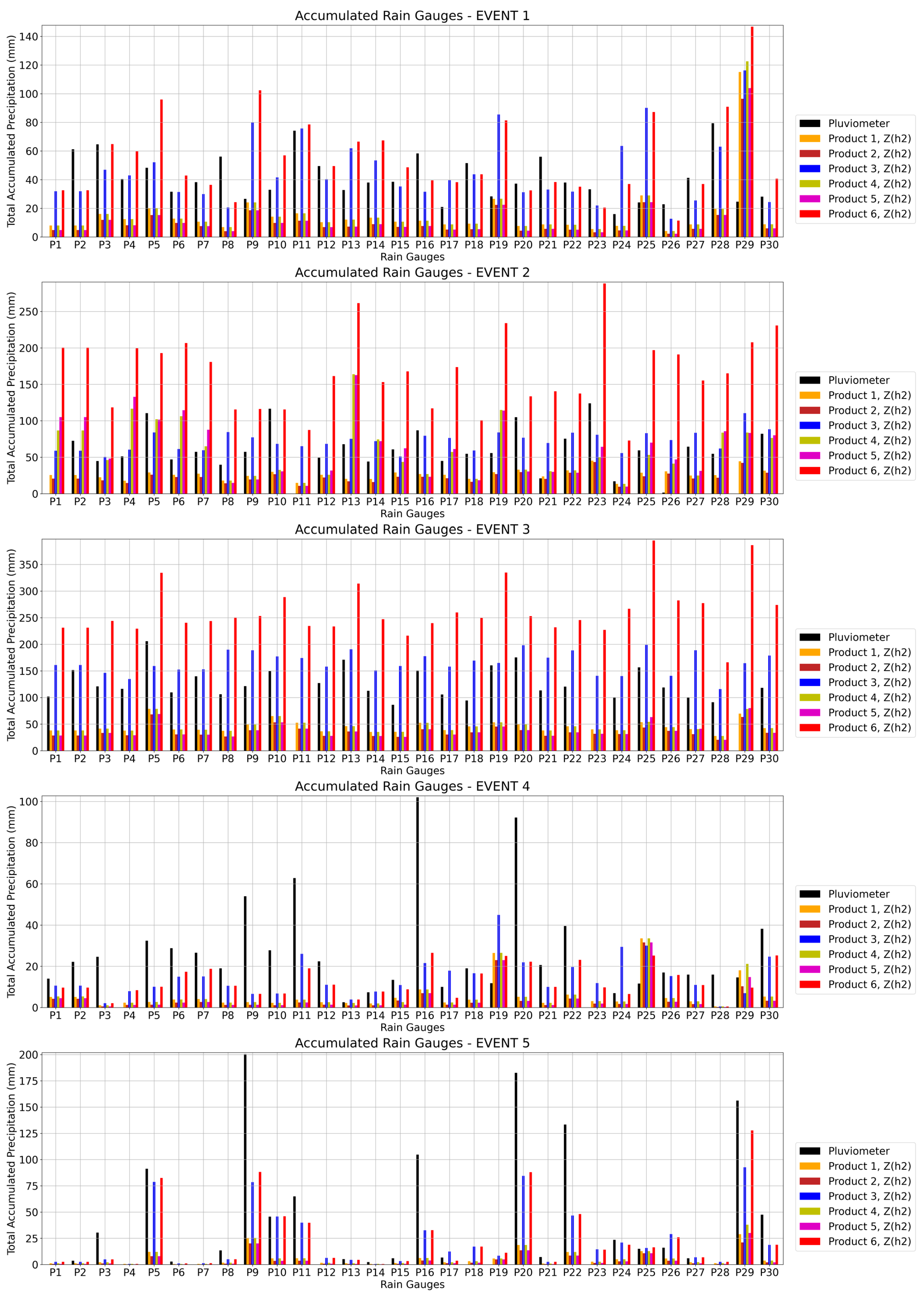
- Product 1: , Marshall–Palmer
- 2
- Product 2: , Morales
- 3
- Product 3: Pluv
- 4
- Product 4: Marshall—Palmer
- 5
- Product 5: MoralesProduct 5 was obtained through the - relationship proposed by Morales Rodriguez [68] (similar to Product 2, with parameters = 378 and = 1.34 in Equation (1)) for low rainfall intensity () and the relationship for higher rainfall intensity (). Similar to Product 4, the algorithm used by Ryzhkov et al. [53] and Wang et al. [61] was also used in this study.
- 6
- Product 6: PluvProduct 6 was also obtained through the - relationship for low rainfall intensity () and the relationship for higher rainfall intensity (). The - relationships were those used in Product 3. Similar to Product 4, the algorithm used by Ryzhkov et al. [53] and Wang et al. [61] was also used in this study.
2.2.3. Rainfall Events Studied
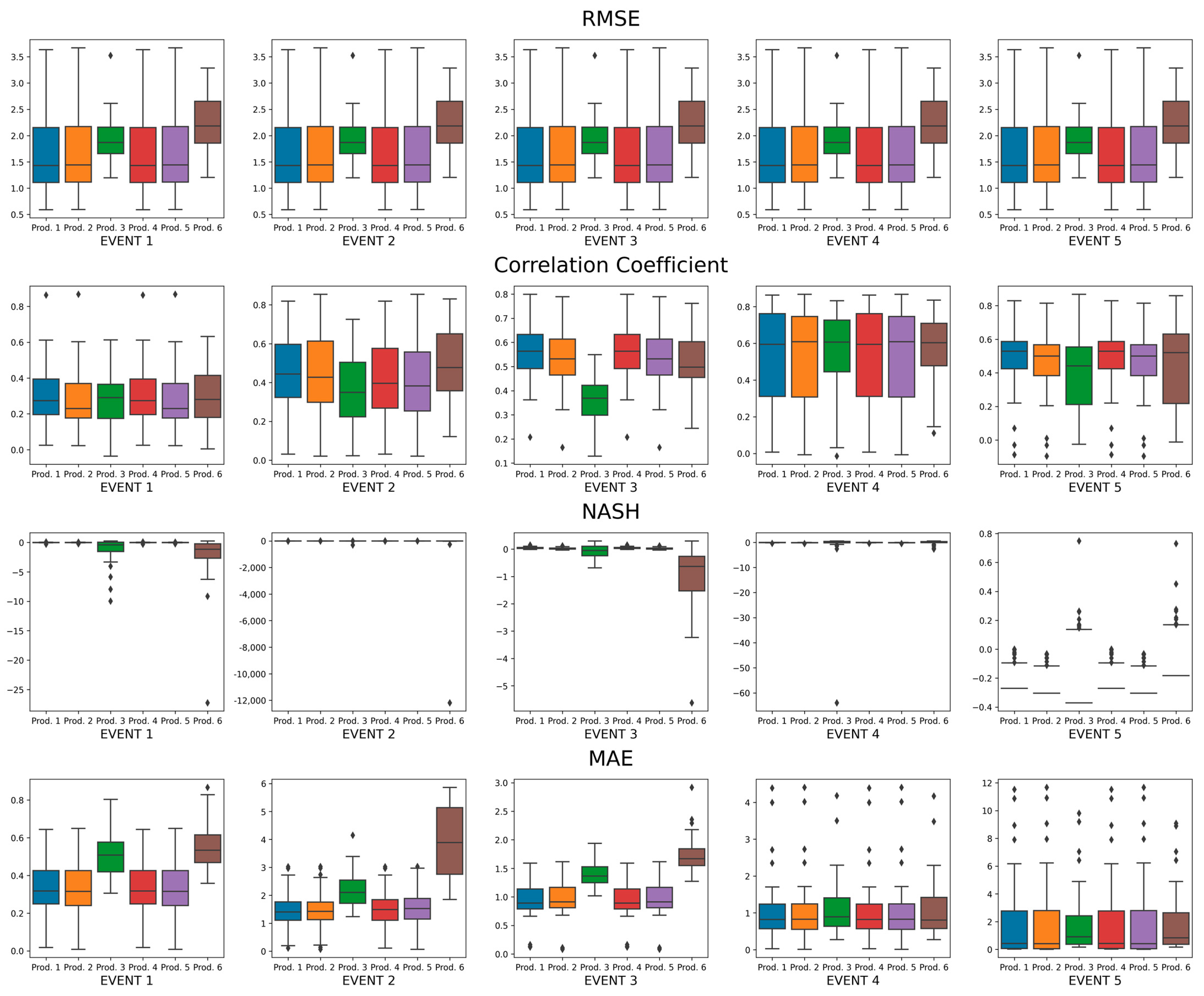
2.3. Statistical Methods
- The Root-Mean-Square Error between actual and predicted time series:
- The Pearson correction coefficient () estimates the strength and direction of the linear relationship between time series:
- The Nash–Sutcliffe efficiency measures how well the outputs of a model reproduce observations against a model that uses only the average of the observed data:
- The mean absolute error between actual and predicted time series:
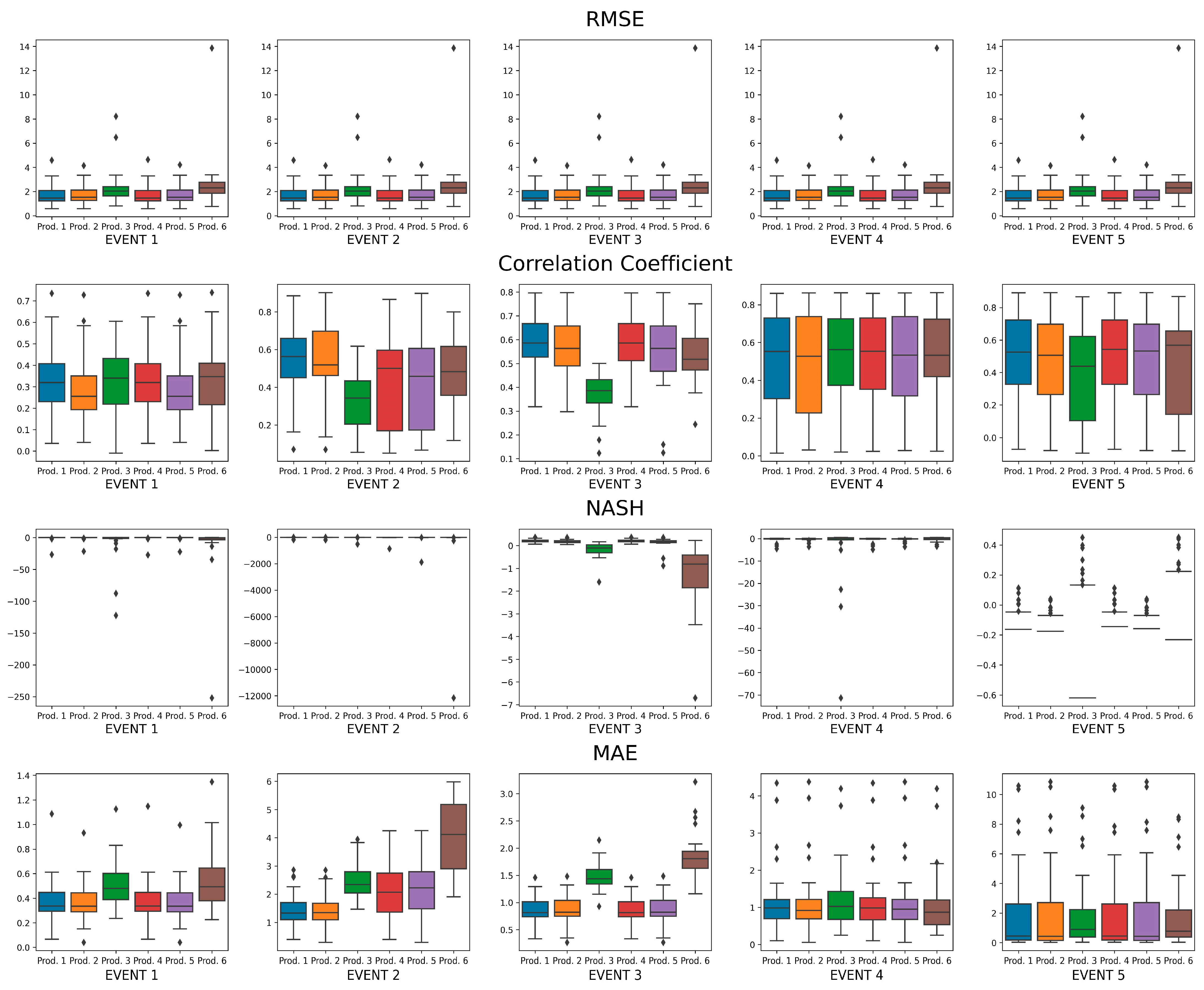
3. Results
3.1. Rain Gauge Data vs. Estimated Rainfall Radar Dara from Reflectivity
3.2. Rain Gauge Data vs. Estimated Rainfall Radar Data from Reflectivity
4. Discussion
Author Contributions
Funding
Data Availability Statement
Acknowledgments
Conflicts of Interest
References
- Schmitt, T.G.; Thomas, M.; Ettrich, N. Analysis and Modeling of Flooding in Urban Drainage Systems. J. Hydrol. 2004, 299, 300–311. [Google Scholar] [CrossRef]
- Chen, J.; Hill, A.A.; Urbano, L.D. A GIS-Based Model for Urban Flood Inundation. J. Hydrol. 2009, 373, 184–192. [Google Scholar] [CrossRef]
- Alves De Souza, B.; Da, I.; Rocha Paz, S.; Ichiba, A.; Willinger, B.; Gires, A.; Carlos, J.; Amorim, C.; De, M.; Reis, M.; et al. Multi-Hydro Hydrological Modelling of a Complex Peri-Urban Catchment with Storage Basins Comparing C-Band and X-Band Radar Rainfall Data. Hydrol. Sci. J. 2018, 63, 1619–1635. [Google Scholar] [CrossRef]
- Celebrini De Oliveira Campos, P.; Da, T.; Rocha Paz, S.; Lenz, L.; Qiu, Y.; Alves, C.N.; Paula, A.; Simoni, R.; Carlos, J.; Amorim, C.; et al. Multi-Criteria Decision Method for Sustainable Watercourse Management in Urban Areas. Sustainability 2020, 12, 6493. [Google Scholar] [CrossRef]
- Qiu, Y.; Da Silva Rocha Paz, I.; Chen, F.; Versini, P.A.; Schertzer, D.; Tchiguirinskaia, I. Space Variability Impacts on Hydrological Responses of Nature-Based Solutions and the Resulting Uncertainty: A Case Study of Guyancourt (France). Hydrol. Earth Syst. Sci. 2021, 25, 3137–3162. [Google Scholar] [CrossRef]
- Loukas, A.; Llasat, M.C.; Ulbrich, U. Preface “Extreme Events Induced by Weather and Climate Change: Evaluation, Forecasting and Proactive Planning. Nat. Hazards Earth Syst. Sci. 2010, 10, 1895–1897. [Google Scholar] [CrossRef] [Green Version]
- Pumo, D.; Arnone, E.; Francipane, A.; Caracciolo, D.; Noto, L.V. Potential Implications of Climate Change and Urbanization on Watershed Hydrology. J. Hydrol. 2017, 554, 80–99. [Google Scholar] [CrossRef]
- Arnone, E.; Pumo, D.; Francipane, A.; La Loggia, G.; Noto, L.V. The Role of Urban Growth, Climate Change, and Their Interplay in Altering Runoff Extremes. Hydrol. Process. 2018, 32, 1755–1770. [Google Scholar] [CrossRef]
- Borges, E.C.; Paz, I.; Leite Neto, A.D.; Willinger, B.; Ichiba, A.; Gires, A.; de Campos, P.C.O.; Monier, L.; Cardinal, H.; Amorim, J.C.C.; et al. Evaluation of the Spatial Variability of Ecosystem Services and Natural Capital: The Urban Land Cover Change Impacts on Carbon Stocks. Int. J. Sustain. Dev. World Ecol. 2020, 28, 339–349. [Google Scholar] [CrossRef]
- Felix, N.B.; de Campos, P.C.O.; Paz, I.; Marques, M.E.S. Geoprocessing Applied to the Assessment of Carbon Storage and Sequestration in a Brazilian Medium-Sized City. Sustain. 2022, 14, 8761. [Google Scholar] [CrossRef]
- Ochoa-Rodriguez, S.; Wang, L.P.; Gires, A.; Pina, R.D.; Reinoso-Rondinel, R.; Bruni, G.; Ichiba, A.; Gaitan, S.; Cristiano, E.; Van Assel, J.; et al. Impact of Spatial and Temporal Resolution of Rainfall Inputs on Urban Hydrodynamic Modelling Outputs: A Multi-Catchment Investigation. J. Hydrol. 2015, 531, 389–407. [Google Scholar] [CrossRef]
- Paz, I.; Willinger, B.; Gires, A.; de Souza, B.A.; Monier, L.; Cardinal, H.; Tisserand, B.; Tchiguirinskaia, I.; Schertzer, D. Small-Scale Rainfall Variability Impacts Analyzed by Fully-Distributed Model Using C-Band and X-Band Radar Data. Water 2019, 11, 1273. [Google Scholar] [CrossRef] [Green Version]
- Lee, J.; Paz, I.; Schertzer, D.; Lee, D.I.; Tchiguirinskaia, I. Multifractal Analysis of Rainfall-Rate Datasets Obtained by Radar and Numerical Model: The Case Study of Typhoon Bolaven (2012). J. Appl. Meteorol. Climatol. 2020, 59, 819–840. [Google Scholar] [CrossRef]
- Cole, S.J.; Moore, R.J. Hydrological Modelling Using Raingauge- and Radar-Based Estimators of Areal Rainfall. J. Hydrol. 2008, 358, 159–181. [Google Scholar] [CrossRef]
- Ochoa-Rodriguez, S.; Wang, L.P.; Willems, P.; Onof, C. A Review of Radar-Rain Gauge Data Merging Methods and Their Potential for Urban Hydrological Applications. Water Resour. Res. 2019, 55, 6356–6391. [Google Scholar] [CrossRef]
- Del Giudice, D.; Honti, M.; Scheidegger, A.; Albert, C.; Reichert, P.; Rieckermann, J. Improving Uncertainty Estimation in Urban Hydrological Modeling by Statistically Describing Bias. Hydrol. Earth Syst. Sci. 2013, 17, 4209–4225. [Google Scholar] [CrossRef] [Green Version]
- Paz, I.; Willinger, B.; Gires, A.; Ichiba, A.; Monier, L.; Zobrist, C.; Tisserand, B.; Tchiguirinskaia, I.; Schertzer, D. Multifractal Comparison of Reflectivity and Polarimetric Rainfall Data from C- and X-Band Radars and Respective Hydrological Responses of a Complex Catchment Model. Water 2018, 10, 269. [Google Scholar] [CrossRef] [Green Version]
- Orellana-Alvear, J.; Célleri, R.; Rollenbeck, R.; Bendix, J. Optimization of X-Band Radar Rainfall Retrieval in the Southern Andes of Ecuador Using a Random Forest Model. Remote Sens. 2019, 11, 1632. [Google Scholar] [CrossRef] [Green Version]
- de Oliveira Campos, P.C.; Paz, I. Spatial Diagnosis of Rain Gauges’ Distribution and Flood Impacts: Case Study in Itaperuna, Rio de Janeiro—Brazil. Water 2020, 12, 1120. [Google Scholar] [CrossRef] [Green Version]
- Villarini, G.; Smith, J.A.; Lynn Baeck, M.; Sturdevant-Rees, P.; Krajewski, W.F. Radar Analyses of Extreme Rainfall and Flooding in Urban Drainage Basins. J. Hydrol. 2010, 381, 266–286. [Google Scholar] [CrossRef]
- Orellana-Alvear, J.; Célleri, R.; Rollenbeck, R.; Muñoz, P.; Contreras, P.; Bendix, J. Assessment of Native Radar Reflectivity and Radar Rainfall Estimates for Discharge Forecasting in Mountain Catchments with a Random Forest Model. Remote Sens. 2020, 12, 1986. [Google Scholar] [CrossRef]
- Paz, I.; Tchiguirinskaia, I.; Schertzer, D. Rain Gauge Networks’ Limitations and the Implications to Hydrological Modelling Highlighted with a X-Band Radar. J. Hydrol. 2020, 583, 124615. [Google Scholar] [CrossRef]
- Krajewski, W.F.; Villarini, G.; Smith, J.A. RADAR-Rainfall Uncertainties: Where Are We after Thirty Years of Effort? Bull. Am. Meteorol. Soc. 2010, 91, 87–94. [Google Scholar] [CrossRef]
- Thorndahl, S.; Nielsen, J.E.; Rasmussen, M.R. Bias Adjustment and Advection Interpolation of Long-Term High Resolution Radar Rainfall Series. J. Hydrol. 2014, 508, 214–226. [Google Scholar] [CrossRef]
- Bringi, V.N.; Chandrasekar, V. Polarimetric Doppler Weather Radar: Principles and Applications; Cambridge University Press: Cambridge, UK, 2001. [Google Scholar] [CrossRef]
- Illingworth, A.J.; Blackman, T.M. The Need to Represent Raindrop Size Spectra as Normalized Gamma Distributions for the Interpretation of Polarization Radar Observations. J. Appl. Meteorol. 2002, 41, 286–297. [Google Scholar] [CrossRef]
- Figueras i Ventura, J.; Boumahmoud, A.-A.; Fradon, B.; Dupuy, P.; Tabary, P. Long-Term Monitoring of French Polarimetric Radar Data Quality and Evaluation of Several Polarimetric Quantitative Precipitation Estimators in Ideal Conditions for Operational Implementation at C-Band. Q. J. R. Meteorol. Soc. 2012, 138, 2212–2228. [Google Scholar] [CrossRef]
- Chandrasekar, V.; Baldini, L.; Bharadwaj, N.; Smith, P.L. Calibration Procedures for Global Precipitation-Measurement Ground-Validation Radars | URSI Journals & Magazine | IEEE Xplore. URSI Radio Sci. Bull. l. 2015, 355, 45–73. [Google Scholar] [CrossRef]
- Hall, W.; Rico-Ramirez, M.A.; Krämer, S. Classification and Correction of the Bright Band Using an Operational C-Band Polarimetric Radar. J. Hydrol. 2015, 531, 248–258. [Google Scholar] [CrossRef] [Green Version]
- INEA—Instituto Estadual de Ambiente. Monitoramento Hidrometeorológico. Available online: http://www.inea.rj.gov.br/ar-agua-e-solo/monitoramento-hidrometeorologico/ (accessed on 7 October 2022).
- IBGE—Instituto Brasileiro de Geografia e Estatística. Portal IBGE Cidades. Available online: https://cidades.ibge.gov.br/brasil/rj/angra-dos-reis/panorama (accessed on 5 October 2022).
- DRM. Carta Geotécnica de Aptidão Urbana-Relatório Consolidado Do Município de Angra Dos Reis. Available online: http://www.drm.rj.gov.br/ (accessed on 11 October 2022).
- DRM-RJ/CPRM. Geologia, Geomorfologia, Geoguímica, Geofísica, Recusos Minerais, Economia Mineral, Hidrogeologia, Estudos de Chuvas Intensas, Aptidão Agrícola, Uso e Cobertura Do Solo, Inventário de Escorregamentos, Diagnóstico Geoambiental. Rio de Janeiro. CPRM: Embrapa Solos: DRM-RJ. Available online: http://www.cprm.gov.br/publique/Gestao-Territorial/Geologia%2C-Meio-Ambiente-e-Saude/Projeto-Rio-de-Janeiro-3498.html (accessed on 11 October 2022).
- Alves, C.N. Previsão de Deslizamento de Encostas a Partir de Modelagem Com Base Física: Estudo de Caso No Município de Angra Dos Reis, Rio de Janeiro; Instituto Militar de Engenharia: Rio de Janeiro, Brazil, 2020. [Google Scholar]
- da Paz, T.S.R.; da Rocha Junior, V.G.; de Campos, P.C.O.; Paz, I.; Caiado, R.G.G.; de Rocha, A.A.; Lima, G.B.A. Hybrid Method to Guide Sustainable Initiatives in Higher Education: A Critical Analysis of Brazilian Municipalities. Int. J. Sustain. High. Educ. 2022; ahead-of-print. [Google Scholar] [CrossRef]
- WMO. Guide to Instruments and Methods of Observation (WMO-No. 8); WMO: Geneva, Switzerland, 2018; Volume I & II, ISBN 978-92-63-10008-5. [Google Scholar]
- Fabry, F. Radar Meteorology: Principles and Practice; Cambridge University Press: Cambridge, UK, 2015; pp. 1–256. [Google Scholar] [CrossRef]
- Rauber, R.M.; Nesbitt, S.W. Radar Meteorology: A First Course; Wiley Blackwell: Hoboken, NJ, USA, 2016; ISBN 9781118432662. [Google Scholar]
- Barnes, S.L. A Technique for Maximizing Details in Numerical Weather Map Analysis. J. Appl. Meteorol. 1964, 3, 396–409. [Google Scholar] [CrossRef]
- Pauley, P.M.; Wu, X. The Theoretical, Discrete, and Actual Response of the Barnes Objective Analysis Scheme for One- and Two-Dimensional Fields. Mon. Weather Rev. 1990, 118, 1145–1164. [Google Scholar] [CrossRef]
- Helmus, J.J.; Collis, S.M. The Python ARM Radar Toolkit (Py-ART), a Library for Working with Weather Radar Data in the Python Programming Language. J. Open Res. Softw. 2016, 4, 25. [Google Scholar] [CrossRef] [Green Version]
- CRESSMAN, G.P. AN OPERATIONAL OBJECTIVE ANALYSIS SYSTEM. Mon. Weather Rev. 1959, 87, 367–374. [Google Scholar] [CrossRef]
- Askelson, M.A.; Aubagnac, J.P.; Straka, J.M. An Adaptation of the Barnes Filter Applied to the Objective Analysis of Radar Data. Mon. Weather Rev. 2000, 128, 3050–3082. [Google Scholar] [CrossRef]
- Zürcher, B.K. Fast Barnes Interpolation. Geosci. Model Dev. Discuss. 2022. [Google Scholar] [CrossRef]
- Marshall, J.S.; Palmer, W.M.K. The Distribution of Raindrops with Size. J. Meteorol. 1948, 5, 165–166. [Google Scholar] [CrossRef]
- Ryzhkov, A.; Zrnić, D.; Atlas, D. Polarimetrically Tuned R ( Z ) Relations and Comparison of Radar Rainfall Methods. J. Appl. Meteorol. 1997, 36, 340–349. [Google Scholar] [CrossRef]
- Ryzhkov, A.; Zhang, P.; Bukovčić, P.; Zhang, J.; Cocks, S. Polarimetric Radar Quantitative Precipitation Estimation. Remote Sens. 2022, 14, 1695. [Google Scholar] [CrossRef]
- Orellana-Alvear, J.; Célleri, R.; Rollenbeck, R.; Bendix, J. Analysis of Rain Types and Their Z–R Relationships at Different Locations in the High Andes of Southern Ecuador. J. Appl. Meteorol. Climatol. 2017, 56, 3065–3080. [Google Scholar] [CrossRef]
- Seliga, T.A.; Bringi, V.N. Potential Use of Radar Differential Reflectivity Measurements at Orthogonal Polarizations for Measuring Precipitation. J. Appl. Meteorol. Climatol. 1976, 15, 69–76. [Google Scholar] [CrossRef]
- Seo, B.C.; Krajewski, W.F.; Ryzhkov, A. Evaluation of the Specific Attenuation Method for Radar-Based Quantitative Precipitation Estimation: Improvements and Practical Challenges. J. Hydrometeorol. 2020, 21, 1333–1347. [Google Scholar] [CrossRef]
- Wijayarathne, D.; Boodoo, S.; Coulibaly, P.; Sills, D. Evaluation of Radar Quantitative Precipitation Estimates (QPEs) as an Input of Hydrological Models for Hydrometeorological Applications. J. Hydrometeorol. 2020, 21, 1847–1864. [Google Scholar] [CrossRef]
- Cifelli, R.; Chandrasekar, V.; Lim, S.; Kennedy, P.C.; Wang, Y.; Rutledge, S.A. A New Dual-Polarization Radar Rainfall Algorithm: Application in Colorado Precipitation Events. J. Atmos. Ocean. Technol. 2011, 28, 352–364. [Google Scholar] [CrossRef] [Green Version]
- Ryzhkov, A.; Diederich, M.; Zhang, P.; Simmer, C. Potential Utilization of Specific Attenuation for Rainfall Estimation, Mitigation of Partial Beam Blockage, and Radar Networking. J. Atmos. Ocean. Technol. 2014, 31, 599–619. [Google Scholar] [CrossRef]
- Maesaka, T.; Iwanami, K.; Maki, M. Non-Negative KDP Estimation by Monotone Increasing PHIDP Assumption below Melting Layer. Seventh Eur. Conf. Radar Meteorol. Hydrol. 2012, p. 2012. Available online: http://www.meteo.fr/cic/meetings/2012/ERAD/extended_abs/QPE_233_ext_abs.pdf (accessed on 1 November 2022).
- Maesaka, T. Operational Rainfall Estimation by X-Band MP Radar Network in MLIT, Japan. In Proceedings of the 35th Conference on Radar Meteorology, Pittsburgh, PA, USA, 26–30 September 2011. [Google Scholar]
- Ryzhkov, A.V.; Zrnic, D.S. Radar Polarimetry for Weather Observations; Springer Atmospheric Sciences, 1st ed.; Springer International Publishing: Cham, Switzerland, 2019; ISBN 978-3-030-05092-4. [Google Scholar]
- Cocks, S.B.; Tang, L.; Zhang, P.; Ryzhkov, A.; Kaney, B.; Elmore, K.L.; Wang, Y.; Zhang, J.; Howard, K. A Prototype Quantitative Precipitation Estimation Algorithm for Operational S-Band Polarimetric Radar Utilizing Specific Attenuation and Specific Differential Phase. Part II: Performance Verification and Case Study Analysis. J. Hydrometeorol. 2019, 20, 999–1014. [Google Scholar] [CrossRef]
- Testud, J.; Le Bouar, E.; Obligis, E.; Ali-Mehenni, M. The Rain Profiling Algorithm Applied to Polarimetric Weather Radar. J. Atmos. Ocean. Technol. 2000, 17, 332–356. [Google Scholar] [CrossRef]
- Tabary, P.; Boumahmoud, A.A.; Andrieu, H.; Thompson, R.J.; Illingworth, A.J.; Bouar, E.L.; Testud, J. Evaluation of Two “ Integrated” Polarimetric Quantitative Precipitation Estimation (QPE) Algorithms at C-Band. J. Hydrol. 2011, 405, 248–260. [Google Scholar] [CrossRef]
- Le Bouar, E.; Testud, J.; Keenan, T.D. Validation of the Rain Profiling Algorithm “ZPHI” from the C-Band Polarimetric Weather Radar in Darwin. J. Atmos. Ocean. Technol. 2001, 18, 1819–1837. [Google Scholar] [CrossRef]
- Wang, Y.; Zhang, P.; Ryzhkov, A.V.; Zhang, J.; Chang, P.L. Utilization of Specific Attenuation for Tropical Rainfall Estimation in Complex Terrain. J. Hydrometeorol. 2014, 15, 2250–2266. [Google Scholar] [CrossRef]
- A-si, Z.; Chao-ying, U.; Shengo, C.; Peng-fei, Z.; Dong-ming, H.; Liu-si, X. Utilization of Specific Attenuation for Rainfall Estimation in Southern China. J. Trop. Meteorol. 2020, 26, 48–61. [Google Scholar] [CrossRef]
- Wang, Y.; Cocks, S.; Tang, L.; Ryzhkov, A.; Zhang, P.; Zhang, J.; Howard, K. A Prototype Quantitative Precipitation Estimation Algorithm for Operational S-Band Polarimetric Radar Utilizing Specific Attenuation and Specific Differential Phase. Part I: Algorithm Description. J. Hydrometeorol. 2019, 20, 985–997. [Google Scholar] [CrossRef]
- Gu, J.Y.; Ryzhkov, A.; Zhang, P.; Neilley, P.; Knight, M.; Wolf, B.; Lee, D.I. Polarimetric Attenuation Correction in Heavy Rain at C Band. J. Appl. Meteorol. Climatol. 2011, 50, 39–58. [Google Scholar] [CrossRef]
- Ryzhkov, A.; Zrnić, D. Assessment of Rainfall Measurement That Uses Specific Differential Phase. J. Appl. Meteorol. 1996, 35, 2080–2090. [Google Scholar] [CrossRef]
- Ryzhkov, A.V.; Giangrande, S.E.; Melnikov, V.M.; Schuur, T.J. Calibration Issues of Dual-Polarization Radar Measurements. J. Atmos. Ocean. Technol. 2005, 22, 1138–1155. [Google Scholar] [CrossRef] [Green Version]
- Beard, K.V.; Chuang, C. A New Model for the Equilibrium Shape of Raindrops. J. Atmos. Sci. 1987, 44, 1509–1524. [Google Scholar] [CrossRef]
- Morales, C.A.R. Distribuição de Tamanho de Gotas de Chuva Nos Trópicos: Ajuste de Uma Função Gamma e Aplicações; Universidade de São Paulo: Sao Paulo, Brazil, 1991. [Google Scholar]
- Sebastianelli, S.; Russo, F.; Adirosi, E.; Napolitano, F.; Baldini, L. A Test Bed for Verification of a Methodology to Correct the Effects of Range Dependent Errors on Radar Estimates. Proceeding of the 7th European Conf. Radar Meteorology and Hydrology, Météo France, Toulouse, France, 24–29 June 2012. [Google Scholar]
- Di Curzio, D.; Di Giovanni, A.; Lidori, R.; Montopoli, M.; Rusi, S. Comparing Rain Gauge and Weather Radar Data in the Estimation of the Pluviometric Inflow from the Apennine Ridge to the Adriatic Coast (Abruzzo Region-Central Italy). 2022. Available online: https://www.preprints.org/manuscript/202211.0051 (accessed on 1 November 2022). [CrossRef]
- Gires, A.; Tchiguirinskaia, I.; Schertzer, D. Pseudo-Radar Algorithms with Two Extremely Wet Months of Disdrometer Data in the Paris Area. Atmos. Res. 2018, 203, 216–230. [Google Scholar] [CrossRef] [Green Version]
- Mie Sein, Z.M.; Ullah, I.; Saleem, F.; Zhi, X.; Syed, S.; Azam, K. Interdecadal Variability in Myanmar Rainfall in the Monsoon Season (May–October) Using Eigen Methods. Water 2021, 13, 729. [Google Scholar] [CrossRef]
- Ullah, I.; Saleem, F.; Iyakaremye, V.; Yin, J.; Ma, X.; Syed, S.; Hina, S.; Asfaw, T.G.; Omer, A. Projected Changes in Socioeconomic Exposure to Heatwaves in South Asia Under Changing Climate. Earth’s Futur. 2022, 10, e2021EF002240. [Google Scholar] [CrossRef]
- Ullah, I.; Ma, X.; Asfaw, T.G.; Yin, J.; Iyakaremye, V.; Saleem, F.; Xing, Y.; Azam, K.; Syed, S. Projected Changes in Increased Drought Risks Over South Asia Under a Warmer Climate. Earth’s Futur. 2022, 10, e2022EF002830. [Google Scholar] [CrossRef]


| ID | Station Name | Lat | Lon |
|---|---|---|---|
| P1 | Angra dos Reis | −22.9785 | −44.2958 |
| P2 | Areal | −22.9820 | −44.2920 |
| P3 | Ariró | −22.9020 | −44.3320 |
| P4 | BNH | −22.9920 | −44.2410 |
| P5 | Bracuí | −22.9330 | −44.3870 |
| P6 | Camorim | −22.9980 | −44.2640 |
| P7 | Camorim Pequeno | −23.0050 | −44.2790 |
| P8 | Enseada | −22.9870 | −44.3200 |
| P9 | Frade | −22.9660 | −44.4400 |
| P10 | Itanema | −22.9230 | −44.3590 |
| P11 | Manbucaba | −22.9510 | −44.5650 |
| P12 | Mombaça | −23.0170 | −44.2910 |
| P13 | Monsuaba | −23.0100 | −44.2220 |
| P14 | Monsuaba 2 | −22.9870 | −44.2180 |
| P15 | Parque do Belém | −22.9604 | −44.2941 |
| P16 | Parque Perequê | −23.0140 | −44.5330 |
| P17 | Ponta Leste | −23.0520 | −44.2430 |
| P18 | Pontal | −22.9480 | −44.3290 |
| P19 | Portogalo | −23.0370 | −44.1950 |
| P20 | Praia Brava | −23.0050 | −44.4800 |
| P21 | Praia da Chacara | −23.0000 | −44.3050 |
| P22 | Praia das Goiabas | −23.0240 | −44.5120 |
| P23 | Praia de Araçatiba | −23.1550 | −44.3270 |
| P24 | Praia de Bananal | −23.1090 | −44.2480 |
| P25 | Praia de Garatucaia | −23.0370 | −44.1770 |
| P26 | Praia Sitio Forte | −23.1370 | −44.2820 |
| P27 | São Bento | −23.0120 | −44.3220 |
| P28 | Serra d’Água | −22.8890 | −44.2780 |
| P29 | Vila do Abraão | −23.1390 | −44.1690 |
| P30 | Vila Velha | −23.0240 | −44.3490 |
| Parameter | Dual-Polarization S-Band Doppler Radar |
|---|---|
| Transmitter | 2.8 GHz |
| Pulse Repetition Frequency (PRF) | 600 Hz |
| Pulse width | 1μsec |
| Pulse Repetition Time (PRT) | 1.67 ms |
| Peak power | 750 kW |
| Antenna gain, horizontal and vertical | 45 dB |
| Antenna aperture | 8.5 |
| Beam width horizontal and vertical | 1° |
| Polarimetric mode | STSR ¹ |
| Nyquist Velocity | 48.195 m/s |
| Number of samples used to compute moments | 60 |
| Radar Receiver Bandwidth | 1 MHz |
| Radar Transmit Power Horizontal and Vertical Channel | 800 watts |
| Scan mode | Plan Position Indicator (PPI) |
| Radial range | 250 km |
| Radar fields 2 | UH, UV, DBZH, DBZV, ZDR, RHOHV, PHIDP, NCPH, NCPV, SNRHC, SNRVC, VELH, VELV, WIDTHH, WIDTHV, CCORH, CCORV |
| Event ID | Event Duration | Number of Rain Gauge Stations | Rain Gauges’ Temporal Resolution | Radar’s Temporal Resolution and Number of Time Steps |
|---|---|---|---|---|
| Event 1 | 14 December 2016 (00:00:00 UTC-3)–18 December 2016 (23:50:00 UTC-3) | 29 1 | 10 min | 10 min (720) |
| Event 2 | 21 January 2017 (00:00:00 UTC-3)–23 January 2017 (23:50:00 UTC-3) | 27 2 | 10 min | 10 min (227) |
| Event 3 | 13 March 2017 (00:00:00 UTC-3)–18 March 2017 (23:50:00 UTC-3) | 27 3 | 10 min | 10 min (720) |
| Event 4 | 12 December 2017 (00:00:00 UTC-3)–13 December 2017 (23:55:00 UTC-3) | 28 4 | 10 min | 5 min (275) |
| Event 5 | 3 July 2018 (00:00:00 UTC-3)–4 July 2018 (23:55:00 UTC-3) | 22 5 | 10 min | 5 min (201) |
Publisher’s Note: MDPI stays neutral with regard to jurisdictional claims in published maps and institutional affiliations. |
© 2022 by the authors. Licensee MDPI, Basel, Switzerland. This article is an open access article distributed under the terms and conditions of the Creative Commons Attribution (CC BY) license (https://creativecommons.org/licenses/by/4.0/).
Share and Cite
Silva, E.J.R.d.; Alves, C.N.; Campos, P.C.d.O.; Oliveira, R.A.A.C.e.; Marques, M.E.S.; Amorim, J.C.C.; Paz, I. Comparison of Rain Gauge Network and Weather Radar Data: Case Study in Angra dos Reis, Brazil. Water 2022, 14, 3944. https://doi.org/10.3390/w14233944
Silva EJRd, Alves CN, Campos PCdO, Oliveira RAACe, Marques MES, Amorim JCC, Paz I. Comparison of Rain Gauge Network and Weather Radar Data: Case Study in Angra dos Reis, Brazil. Water. 2022; 14(23):3944. https://doi.org/10.3390/w14233944
Chicago/Turabian StyleSilva, Elton John Robaina da, Camila Nascimento Alves, Priscila Celebrini de Oliveira Campos, Raquel Aparecida Abrahão Costa e Oliveira, Maria Esther Soares Marques, José Carlos Cesar Amorim, and Igor Paz. 2022. "Comparison of Rain Gauge Network and Weather Radar Data: Case Study in Angra dos Reis, Brazil" Water 14, no. 23: 3944. https://doi.org/10.3390/w14233944