
Large Eddy Simulation of Compound Open Channel Flows with Floodplain Vegetation
by
 ,
,
Cheng Zeng
1,
Yimo Bai
1,
Jie Zhou
2,*,
Fei Qiu
1,
Shaowei Ding
3,
Yudie Hu
1 and
Lingling Wang
1 1
College of Water Conservancy and Hydropower Engineering, Hohai University, Nanjing 210098, China
2
College of Mechanics and Materials, Hohai University, Nanjing 211100, China
3
China Design Group Co., Ltd., Nanjing 210014, China
*
Author to whom correspondence should be addressed.
Water 2022, 14(23), 3951; https://doi.org/10.3390/w14233951
Submission received: 30 October 2022
/
Revised: 30 November 2022
/
Accepted: 1 December 2022
/
Published: 4 December 2022
(This article belongs to the Special Issue Hydraulics of River Networks and Modelling)
Abstract
:Floodplain vegetation is of great importance in velocity distribution and turbulent coherent structure within compound open channel flows. As the large eddy simulation (LES) technique can provide detailed instantaneous flow dynamics and coherent turbulent structure predictions, it is of great importance to perform LES simulations of compound open channel flows with floodplain vegetation. In the present study, a wall-modeled large eddy simulation (WMLES) method was employed to simulate the compound open channel flows with floodplain vegetation. The vegetation-induced resistance effect was modeled with the drag force method. The WMLES model, incorporating the drag force method, was verified against flume measurements and an analytical solution of vegetated open channel flows. Numerical simulations were conducted with a depth ratio of 0.5 and four different floodplain vegetation densities (frk = 0, 0.28 m−1, 1.13 m−1 and 2.26 m−1). The main flow velocity, secondary flow, bed shear stress and vortex coherent structure, based on the Q criterion, were obtained and analyzed. Based on the numerical results, the influences of floodplain vegetation density on the flow field and turbulent structure of compound open channel flows were summarized and discussed. Compared to the case without floodplain vegetation, the streamwise velocity in the main channel increased by 10.8%, 19.9% and 24.4% with the frk = 0.28 m−1, 1.13 m−1 and 2.26 m−1, respectively. The results also indicated that, when the floodplain vegetation density increased, the following occurred: the velocity increased in the main channel, while the velocity decreased in the floodplain; the transverse momentum exchange was enhanced; and the strip structures were more concentrated near the junction area of compound open channel flows.
1. Introduction
A variety of aquatic vegetation exists in natural rivers and lakes, and plant communities interact with water flows to form a diversified ecological water environment [1]. The existence of aquatic vegetation can not only change the velocity distribution and turbulent structure of water flows, but can also affect the migration of sediments and pollutants. When a river is covered with aquatic plants, there are obvious velocity gradients in horizontal, transverse and vertical directions while the water flows through the vegetation. Most natural and restored waterways, at a minimum, are composed of a main channel and one or more adjacent floodplains, which are termed compound open channel flows. Compound open channel flows are characterized by a complex flow field and turbulent structure because of the interaction between the main channel and the floodplain. With the existence of floodplain vegetation, the difference in the mean velocities between the main channel and floodplain is enhanced. The flow field and turbulent structure of compound open channel flows are much more complicated with floodplain vegetation and need to be further studied. Furthermore, it is worth noting that the vegetation has been considered as a retrofitting solution for flood mitigation in low-lying coastal areas [2,3]. Aquatic plants have also been used as a retrofitting solution to mitigate overtopping from seawalls [4].
Considerable attention has been attracted to the investigation of the hydrodynamics of compound open channel flows with floodplain vegetation, including physical and numerical modeling. Noat et al. [5] established a three-dimensional (3-D) model, utilizing the algebraic stress model (ASM), to replicate compound open channel flows with floodplain vegetation. The effects of the cross-section shape on the flow patterns were identified, based on their numerical results. Kang and Choi [6] conducted numerical simulations of compound open channel flows with floodplain vegetation by using Reynolds stress model (RSM). A depth-averaged analysis was performed to investigate momentum exchange along the lateral direction. Yang et al. [7] conducted flume experiments to investigate the effects of different kinds of floodplain vegetation on the turbulence characteristics of compound open channel flows. Zhang et al. [8] established a two-dimensional (2-D) Reynolds averaged Navier–Stokes (RANS) model to simulate the turbulent structure in open channels with partially distributed vegetation. A good agreement was obtained between the numerical results and the experimental measurements. Cui and Neary [9] conducted a large eddy simulation (LES) study on the turbulent structure of compound open channel flows with submerged vegetation. Compared to the RANS model, the LES model could effectively simulate the impact of submerged vegetation on the mean flow field and resolve coherent structures observed in the instantaneous flow field. Sun and Shiono [10] physically studied the turbulent structure of compound open channel flows with one-line emergent vegetation along the interface edge. The velocity distribution, discharge ratio and bed shear stress were found to be significantly different from those with no vegetation. Huai et al. [11] successfully established a 2-D analytical solution model based on the effect of vegetation on the water flow structure of compound open channel flows with floodplain vegetation. Zhang et al. [12] numerically investigated the flow structure, the velocity distribution and mass transport process in a straight compound open channel with a 3D non-linear k-ε turbulence model. Zhang [13] carried out flume experiments to reveal the impact of emergent and submerged floodplain vegetation on flow structure of compound open channel flows. Zeng and Li [14] physically and numerically investigated the interaction between current and vegetation patches. Zeng et al. [15] experimentally investigated the ejection and sweep phenomenon caused by the floodplain vegetation variation with quadrant analysis. Dupuis et al. [16] conducted flume experiments to investigate the longitudinal development of the mixing layer within the interface area of compound open channel flows with floodplain vegetation. They reported that the effort of the secondary flow is significant in the redistribution of longitudinal momentum in the compound open channel flows. Barman and Kumar [17] physically collected the turbulent measurements in the heterogeneous canopy within the floodplain area of compound open channels. The differences of flow properties were identified, compared to the cases with homogeneous floodplain vegetation. As a new approach, Smoothed Particle Hydrodynamics (SPH) was applied to simulate the seagrass movement under waves and currents [18]. The SPH model was also successfully applied to simulate the flow characteristics in turbulent open channel flows through the porous bed with rough interfacial boundaries [19].
In flood modeling, compared to the results of Gaussian Process models [20], the LES simulations could provide detailed instantaneous flow dynamics and coherent turbulent structure predictions. Recent studies [21,22] demonstrated that the LES technique is robust and reliable for the modeling of open channel flows. However, the accuracy of LES results is determined by the grid resolution in the boundary layer, which normally leads to high computational cost. As a useful extension of the LES technique, the wall-modeled large eddy simulation (WMLES) model proved to be able to accurately simulate the wall-bounded turbulent flows with smaller grid requirements in the boundary layers. Due to the lower cost, the WMLES model attracted more and more attention in LES modeling. Zeng et al. [22] developed a 3-D model with the WMLES technique to simulate the flow field and turbulent structure of compound open channel flows. The model was well validated with existing experimental measurements and previous conventional LES results. The grid number of the WMLES model was found to be 1/8~1/3 of that in previous LES simulations [23,24]. The model was successfully applied to investigate the influence of the depth ratio (hr, defined as the ratio of the water depth in the floodplain and the water depth in the main channel) on the flow field and turbulent structure [25], and the distributions of energy and momentum correction coefficients in compound open channel flows [26]. In the present study, the WMLES model was applied to simulate the compound open channel flows with floodplain vegetation. The drag force method was adopted to model the resistance effect of vegetation. The WMLES model, incorporating the drag force method, was verified against flume measurements and an analytical solution of vegetated open channel flows. Numerical simulations were conducted with four different vegetation densities (frk = 0, 0.28 m−1, 1.13 m−1 and 2.26 m−1). Based on the numerical results, the influence of floodplain vegetation density on the flow field and turbulent structure of compound open channel flows was studied and summarized.
2. Mathematical Model
2.1. Governing Equations
The incompressible Navier–Stokes equations were solved with the WMLES method in the simulations conducted. The basic idea of LES is to filter the vortices spatially with a filter function. While the small-scale vortices were modeled with the sub grid scale (SGS) stress model, large-scale vortices were resolved with the filtered incompressible Navier–Stokes equations. The filtered governing equation is shown as follows:
where xi represents the Cartesian coordinates (i, j = 1, 2, 3 corresponding to x, y and z, meaning the streamwise, vertical and spanwise directions, respectively); and (i, j = 1, 2, 3) are the filtered velocity components; t is the time; is the filtered pressure; is the gravitational acceleration component in the xi direction, g is the gravitational acceleration and θ is the angle of the channel to the horizontal. The term τij in Equation (2) is the SGS stress tensor. In the present study, the Boussinesq’s Hypothesis was employed to calculate the SGS stress tensor as:
where Sij is the strain rate tensor and μt is the sub grid scale turbulent viscosity which can be modeled as:
where dw is the nearest wall distance, Ωij is the rotation rate tensor, κ = 0.41, Cs = 0.2, and y+ is the normal to the wall inner scaling. Based on a modified grid scale, the WMLES model considers the grid anisotropy in wall-modeled flows:
where hmax is the maximum length of the cell edge; hwn is the normal grid spacing and Cw = 0.15 is a constant.
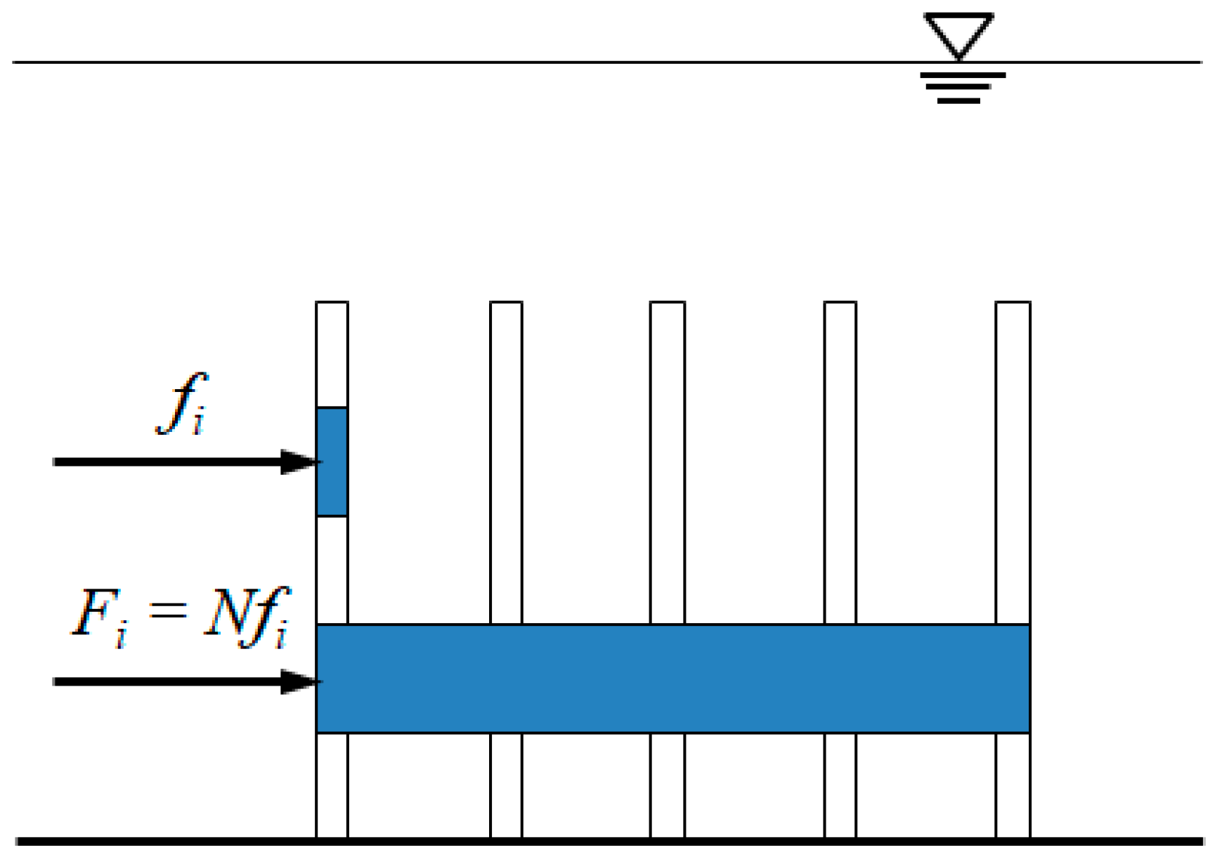
In the present study, the drag force method was used to simulate the resistance effect of floodplain vegetation. The resistance effect of floodplain vegetation was modeled with the quadratic friction law. If a single stem was considered, as shown in Figure 1, the force per unit depth could be obtained by:
in which ρ is density; Cd is the drag coefficient of stem; bv is the width of stem. The average force per unit volume within the vegetated floodplain could be calculated as:
in which Fi (=Fx, Fy, Fz = 0) are the resistance force components per unit volume induced by vegetation in x, y, z directions, N = number density and the resistance parameter frk = CdbvN. The resistance parameter frk can be used to characterize the influence of vegetation density on water flow. The value of Cd of circular cylinder rods was found to be inconstant. Previous studies [27] suggested that the Cd-value was in the range of 1.13 ± 0.15. In the present simulations, the Cd-value was taken as 1.13.
2.2. Boundary Condition and Numerical Algorithm
In the present simulations, the rigid-lid assumption was imposed for the upper boundary. The assumption has been widely applied in previous LES simulations of compound open channel flows [24,28]. The bed and sidewall of the compound open channel were set as the no-slip boundary condition. At the inlet and outlet boundaries, the periodic boundary condition was employed. The model details and validation case study can be found in Zeng et al. [22].
Numerical algorithms which do not produce significant artificial viscosity are required for the LES simulations. The Spectral method [29] and the Finite Volume Method (FVM) are widely used in solving the governing Equations (1) and (2). According to the existing studies [30,31], the spectral method needs substantially more CPU time and RAM, as compared with the FVM, for simple geometries. In order to save computational costs, the governing equations were discretized with the FVM in the present simulations. The pressure–velocity coupling was performed using the pressure implicit with the splitting of operators (PISO) algorithm. The convection and diffusion terms were discretized using the third-order quadratic upstream interpolation for convective kinematics (QUICK) scheme.
3. Verification of Drag Force Method
3.1. Simulation Implementation
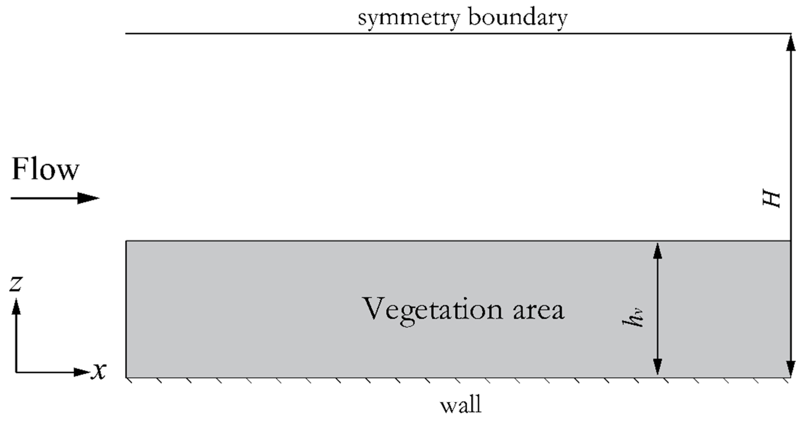
The drag force method was verified with the flume experiments of Dunn et al. [27]. The experiments were carried out in a rectangular flume, which was 19.5 m in length. The width (W) and water depth (H) of the rectangular cross-section were 0.91 m and 0.61 m, respectively. The physical model parameters are listed in Table 1. Q is the discharge rate, and S0 is the bed slope. The simulation area of the verification case was of length 2 m, width 0.91 m and height 0.61 m. The vegetation height hv was 0.1175 m. The schematic diagram of the longitudinal section of the simulation area is shown in Figure 2. A hexahedral structured grid was used, and the total number of grids was 384,000.
In the present simulations, the steady velocity field, computed with the SST k-ε model, was set as the initial condition to reach a fully developed turbulent state quickly. Statistics were performed when a fully developed turbulent state was reached after 50 flow cycles (one flow cycle was equal to 10 H/Um, in which H was the water depth and Um was the bulk velocity).
3.2. Case Verification
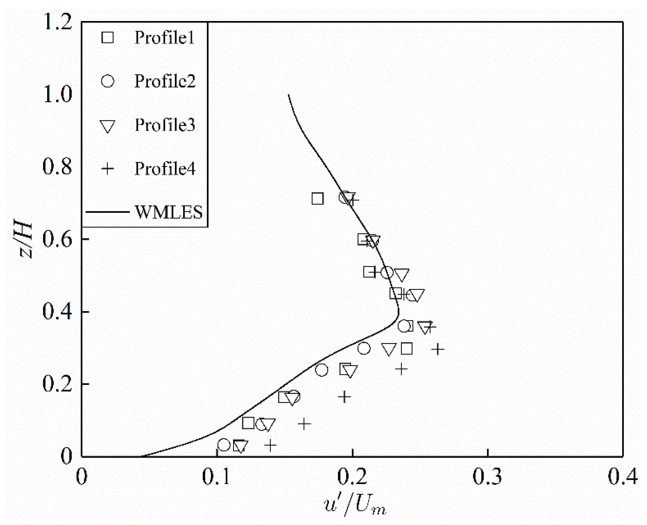
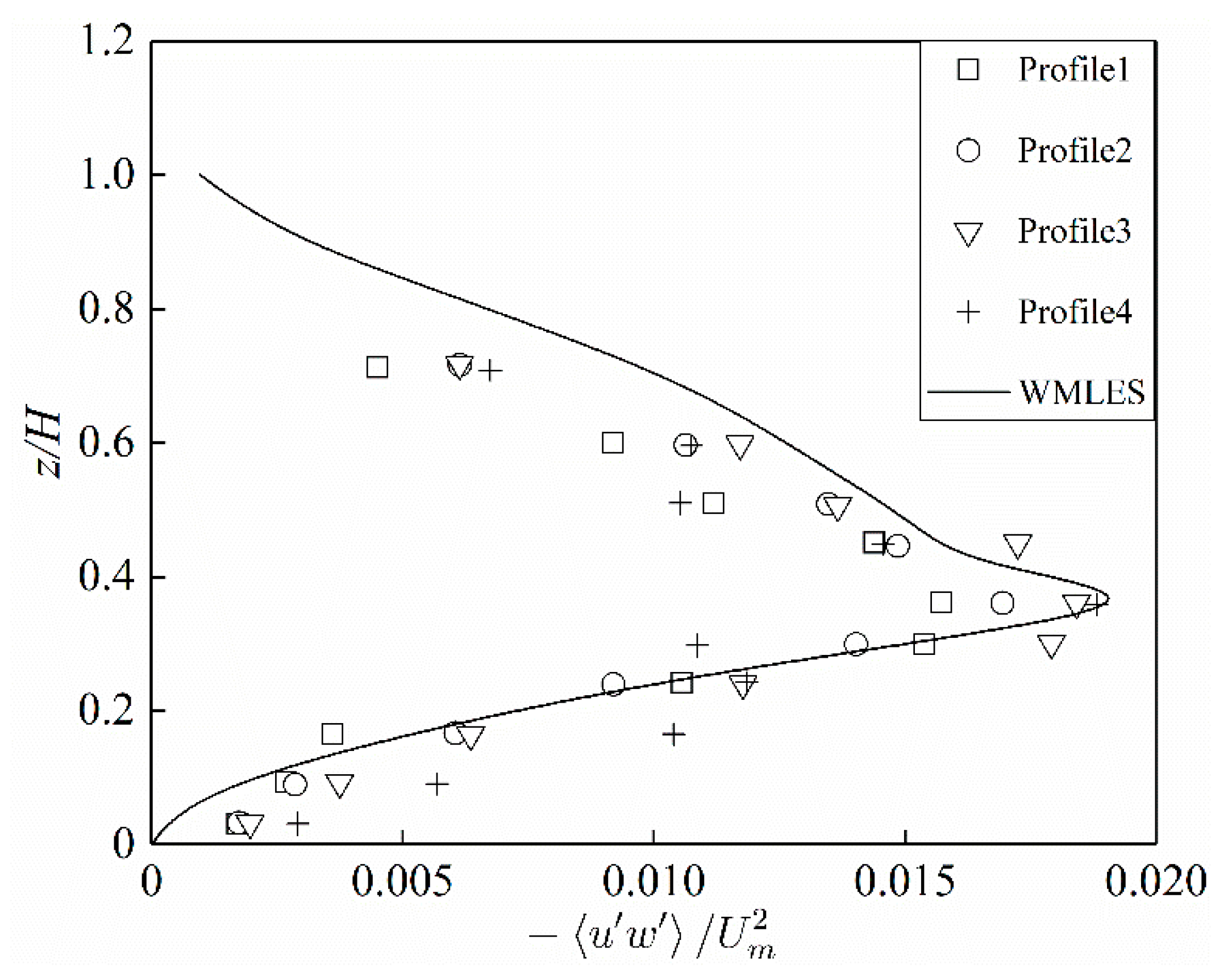
Figure 3, Figure 4 and Figure 5 show the streamwise velocities, fluctuation velocities and Reynolds stress, respectively. The plots are non-dimensionalized with the mean velocity of cross section Um. Figure 3 shows that the vertical profile of time-averaged streamwise velocity. The experimental measurements and the analytical results are plotted in the figure. For the empirical and quasi-theoretical analysis, the vegetation resistance was usually parameterized with the Darcy–Weisbach friction factor [32]. Kouwen [33] proposed a rational method to estimate the roughness coefficient for flow over submerged vegetation. In the present study, the analytical model of Huai et al. [34] was employed for comparison. For the flow layer within vegetation, the velocity could be calculated as:
where α is a constant and taken as 20.7. For the upper non-vegetated flow, the velocity could be calculated as:
where l0 is the mixing length at the interface between vegetation layer and the upper non-vegetated flow layer and can be obtained by referring to the region suggested by Righetti and Armanini [35], U* is the shear velocity and equal to:
From Figure 3, it can be seen that the computational results agreed well with the experimental data and the analytical solution. The error between the experimental measurements and the analytical results might be attributed to neglecting the wake effect of the vegetation stems.
As can be seen in Figure 4 and Figure 5, the numerical results of fluctuation velocity and Reynolds stress were slightly different from the experimental results. This might be attributed to the fact that the porous media model considers macroscopic vegetation, but the influence of the community on the flow does not reflect the effect of a single stem on the flow field and the turbulence characteristics of the water flow within the vegetation community. Due to vegetation roughness, the distribution of streamwise velocity in the vertical z direction no longer conforms to the law of logarithmic distribution. While the resistance effect within the lower vegetation region increased, the flow velocity decreased within the vegetation layer and assumed an S-shaped distribution. It gradually increased along the vertical direction and showed a J-shaped distribution. It can be found from these figures that there was a large velocity gradient between the flow in the vegetation area and the upper flow in the non-vegetation area. A shear layer could be observed at the top of the vegetation canopy. Therefore, maximum values of Reynolds stress and fluctuating velocity appeared near the top of the vegetation canopy, and the Reynolds stress and fluctuating velocity decreased approaching the water surface and the channel bottom.
These comparisons indicated that the computational results agreed fairly well with the experimental measurements. It could be concluded that the WMLES model, incorporating the drag force method, performed well in the modeling of vegetated open channel flows.
4. Computational Cases
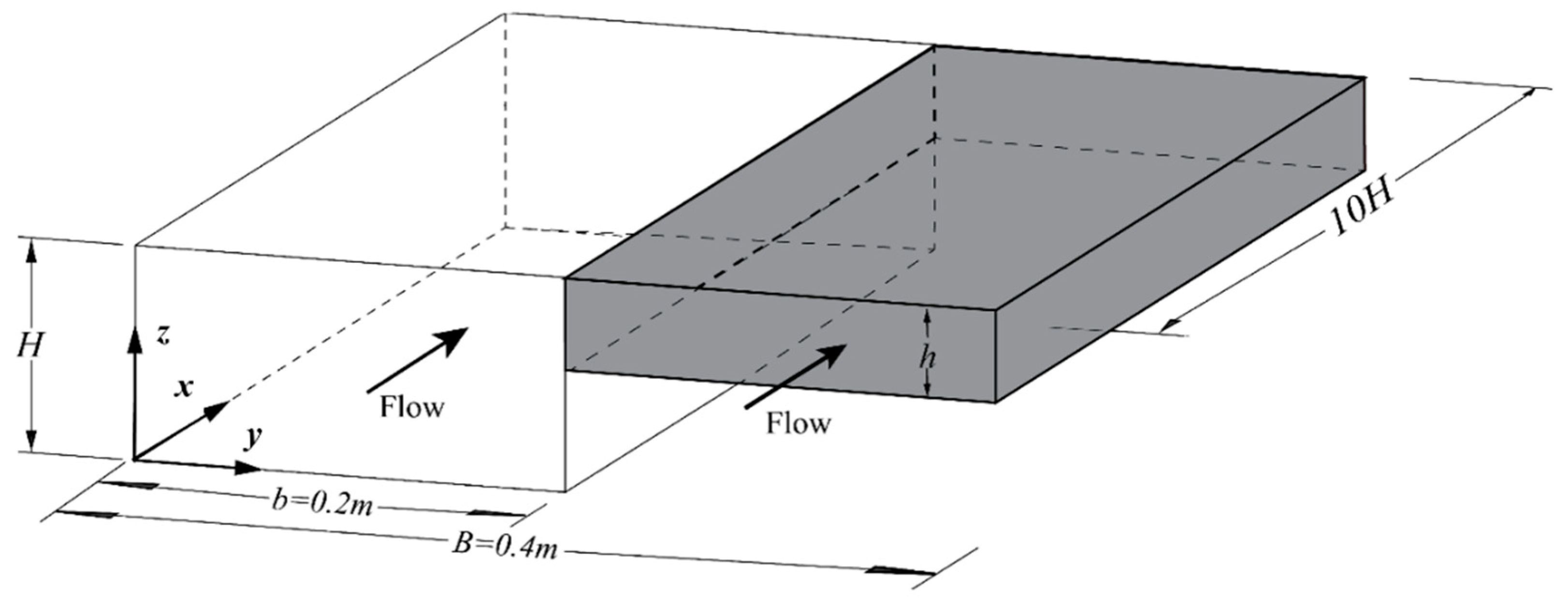
In the present study, the WMLES simulations were performed for compound open channel flows with hr = 0.5. The computational domain is shown in Figure 6. The width of compound channel B was 0.4 m and the width of the main channel b was 0.2 m. The depth of the main channel H was 0.08 m and the depth of the floodplain h was 0.04 m. A hexahedral structured grid was used in the present simulation, and the grid size was uniform in the streamwise, spanwise and vertical directions. The total number of grids was 1,920,000.
The resistance effect of floodplain vegetation was modeled with the drag force method. The vegetation height hv was set to the water depth within the floodplain. Three cases, with different floodplain vegetation densities, were set. The resistance parameters frk in these three cases were 0.28 m−1, 1.13 m−1 and 2.26 m−1, respectively. Boundary conditions adopted in the present simulations were the same as previous simulations without floodplain vegetation [25]. To facilitate the comparative analysis in the present study, the computational results of the floodplain without floodplain vegetation were also included for comparison. Thus, there were four cases, with vegetation densities of 0, 0.28 m−1, 1.13 m−1 and 2.26 m−1, considered in the present study. The impact of floodplain vegetation on the sectional velocity distribution, secondary currents, bed shear stress, Reynolds stress and turbulent structure was analyzed and summarized.
5. Results
In the analysis of results, statistics were produced for roughly 60 flow cycles when the fully developed turbulent state was reached after 50 flow cycles. To efficiently analyze the computational results, the length, width and height were non-dimensionalized with the water depth of the main channel H. The values U, V, and W were the time-averaged velocity components in the x, y and z directions, respectively. and were the three fluctuating velocity components in the x, y and z directions, respectively.
5.1. Flow Field and Secondary Flow
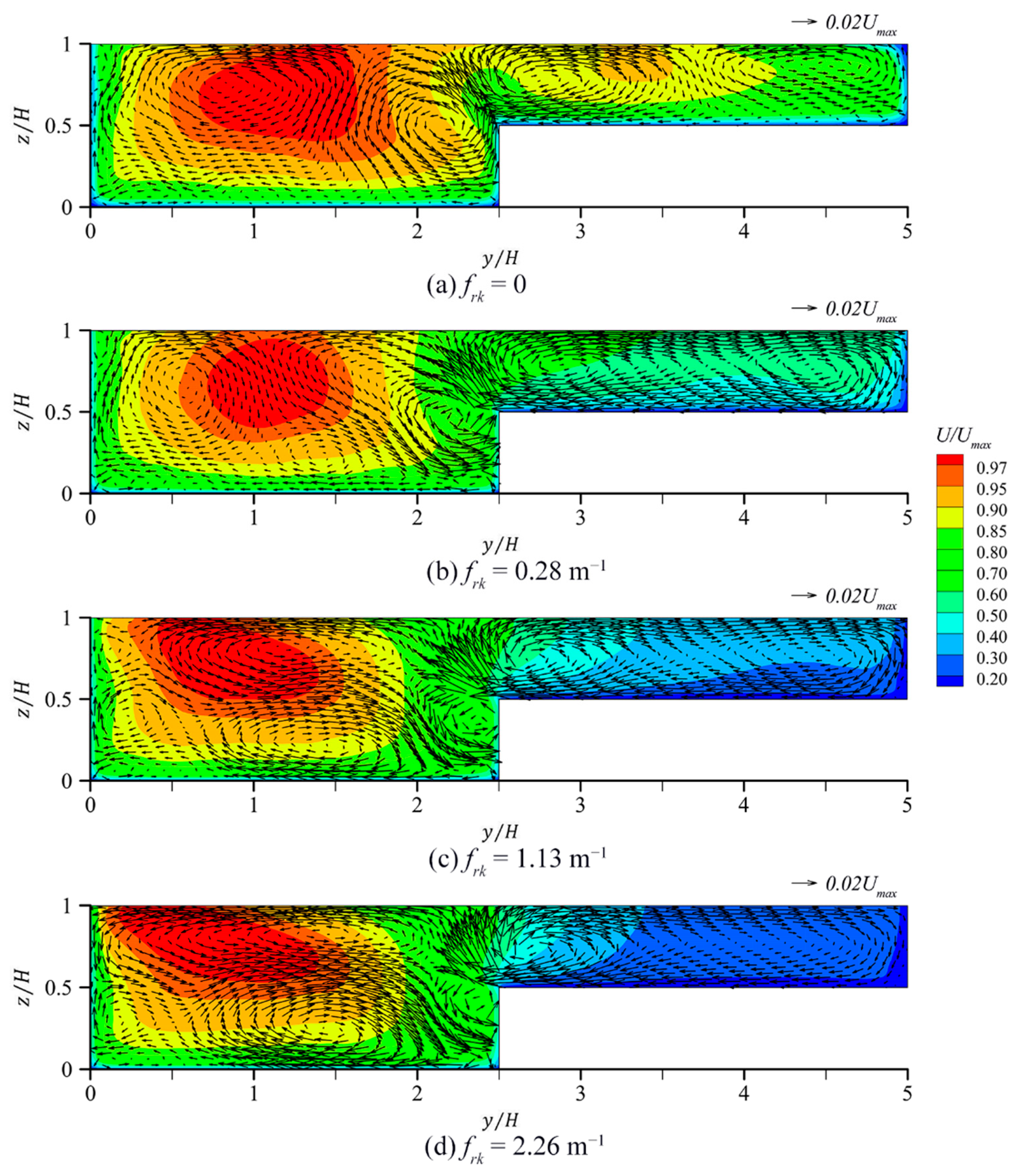
Figure 7 shows the sectional distribution of the streamwise velocity U and the secondary current vectors (V, W) with different vegetation densities. With increase of the floodplain vegetation density, the streamwise velocity in the floodplain decreased, the streamwise velocity in the main channel increased, and the velocity gradient at the junction area increased. Compared to the case without floodplain vegetation, the streamwise velocity in the main channel increased by 10.8%, 19.9% and 24.4%, and the streamwise velocity in the floodplain decreased by 24.5%, 45.2% and 55.5% with the frk = 0.28 m−1, 1.13 m−1 and 2.26 m−1, respectively. Within the four cases of different floodplain vegetation densities, the location of the maximum streamwise velocity appeared in the main channel, and the smallest streamwise velocity was observed within the floodplain. With the increases of floodplain vegetation density, the high velocity area approached the side wall of the main channel, and the maximum velocity position moved toward the corner of the side wall and the water surface of the main channel. Although the computational flow field and secondary flow in this paper were generally consistent with the numerical simulation results of ASM [5], the present numerical model could faithfully replicate the velocity dip phenomena, while the phenomena were not observed in the results of ASM. It is worth noting that when the resistance parameter frk was 1.13 m−1, the characteristics of the flow field were similar to those when frk was 2.26 m−1, indicating that, when the vegetation density increased to a certain value, the floodplain vegetation tended to completely obstruct the water flow, and the flow field characteristics were less affected by the vegetation density.
When the resistance parameter frk was 0.28 m−1, 1.13 m−1 and 2.26 m−1, the maximum value of the secondary flow velocity was 4.4%, 4.8% and 5.8% of the maximum streamwise velocity, respectively. When the vegetation density increased, the intensity of the secondary flow near the junction area gradually increased, which also indicated that the presence of the floodplain vegetation enhanced the intensity of the secondary flow. In the main channel, the vortex close to the junction gradually approached the side wall due to the secondary flow, and the range of vortex scale reduced. When the floodplain vegetation density increased, the vortex near the bottom of the main channel became more obvious. The vortex at the water surface of the main channel evolved from two vortices in opposite directions to one vortex. The intensity of the floodplain vortex which was close to the interface became larger.
5.2. Bed Shear Stress
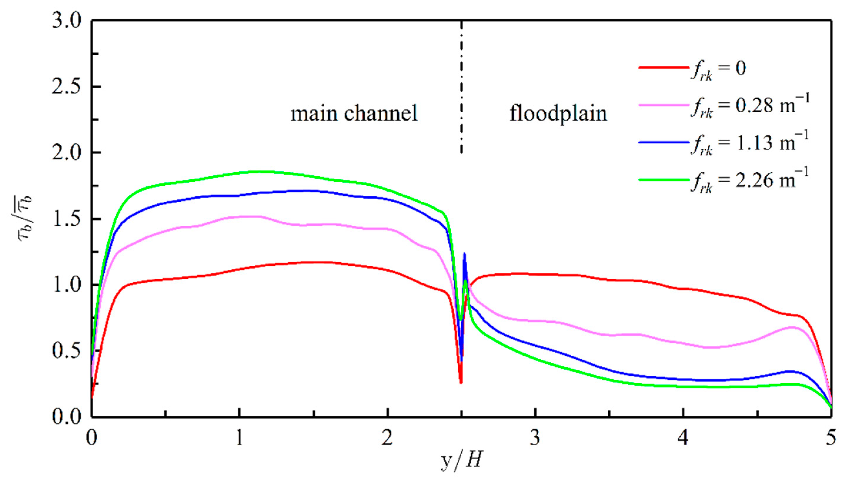
Figure 8 displays the distribution of the dimensionless bed shear stress with four different vegetation densities. As a result of the vegetation-induced drag effect, the flow velocity of the floodplain decreased and the flow velocity of the main channel increased, resulting in an increase for the bed shear stress on the main channel and a decrease on the floodplain. With the increase of floodplain vegetation density, the bed shear stress at the bottom of the floodplain decreased, and the bed shear stress at the bottom of the main channel increased. With the increase of the velocity gradient within the interface area, the bed shear stress changed more sharply. The WMLES results were approximately consistent with the previous numerical results [5,6]. However, the bed shear stress calculated by WMLES within the junction area was relatively flat compared to the previous results. It could be deduced that, with the existence of the floodplain vegetation, the erosion of the floodplain weakened. On the contrary, the erosion to the main channel bottom increased because of the increase of the bed shear stress. Therefore, if the floodplain is roughened with vegetation, the discharge rate of the compound open channel is reduced, which is not safe for flood control. However, the bed shear stress of the floodplain is significantly reduced, which is helpful for the protection of the floodplain. Thus, when the floodplain is multipurpose, it is necessary to comprehensively consider its impact on many factors, such as flood control and floodplain protection.
5.3. Reynolds Stress
The dimensionless Reynolds stress with the four different floodplain vegetation densities are displayed in Figure 9. With the existence of floodplain vegetation, the positive area of the Reynolds stress closing to the junction in the floodplain disappeared. When the resistance parameter frk was 0.28 m−1, the Reynolds stress along the vertical direction was 0 at y/H = 1. With an increase in vegetation density, the zero-contour approached the side wall of main channel, while the absolute value of the Reynolds stress reached its maximum value near the interface area of the compound open channel flows. When the vegetation density increased, the Reynolds stress gradually increased near the interface area of compound open channel flows.
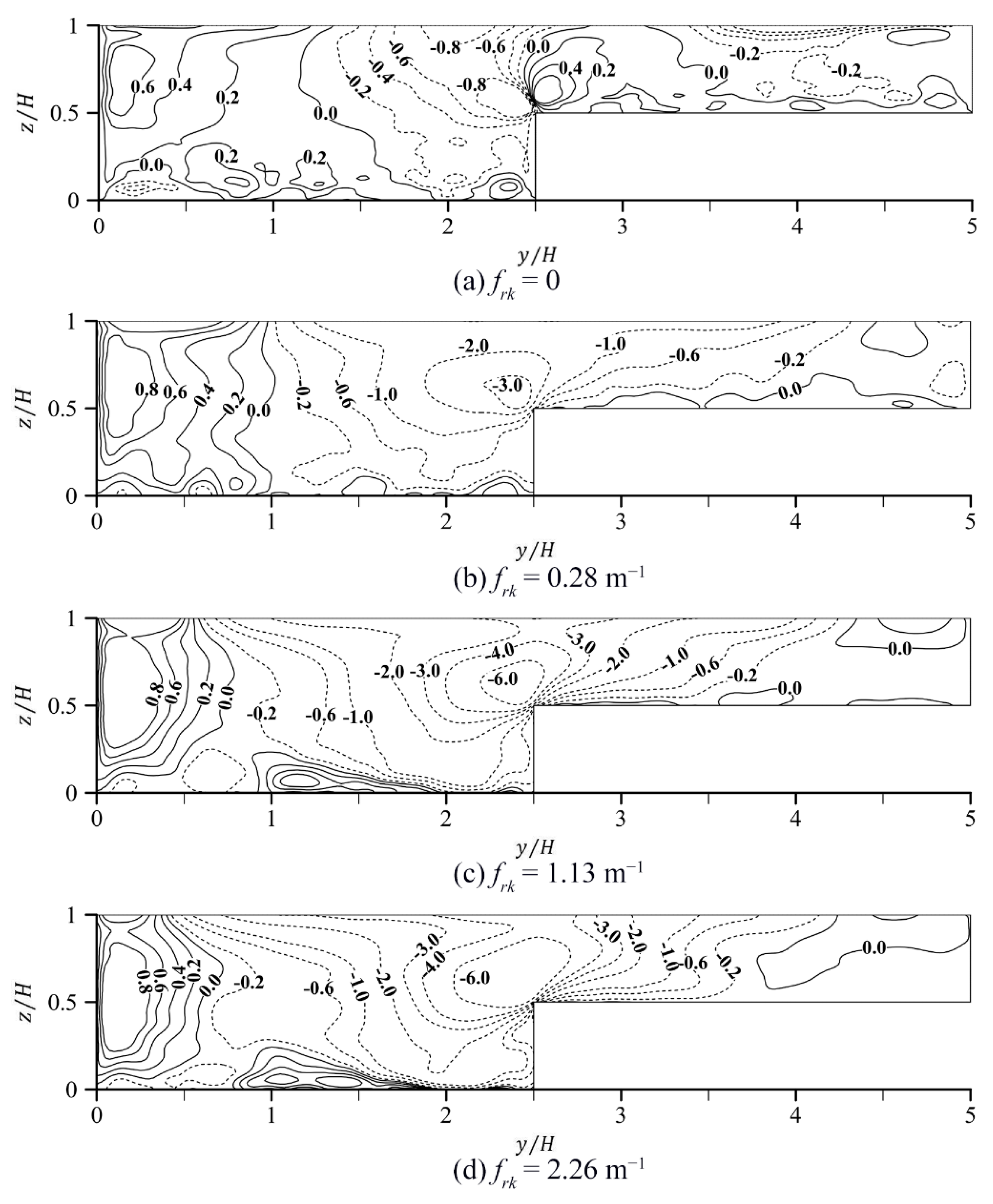
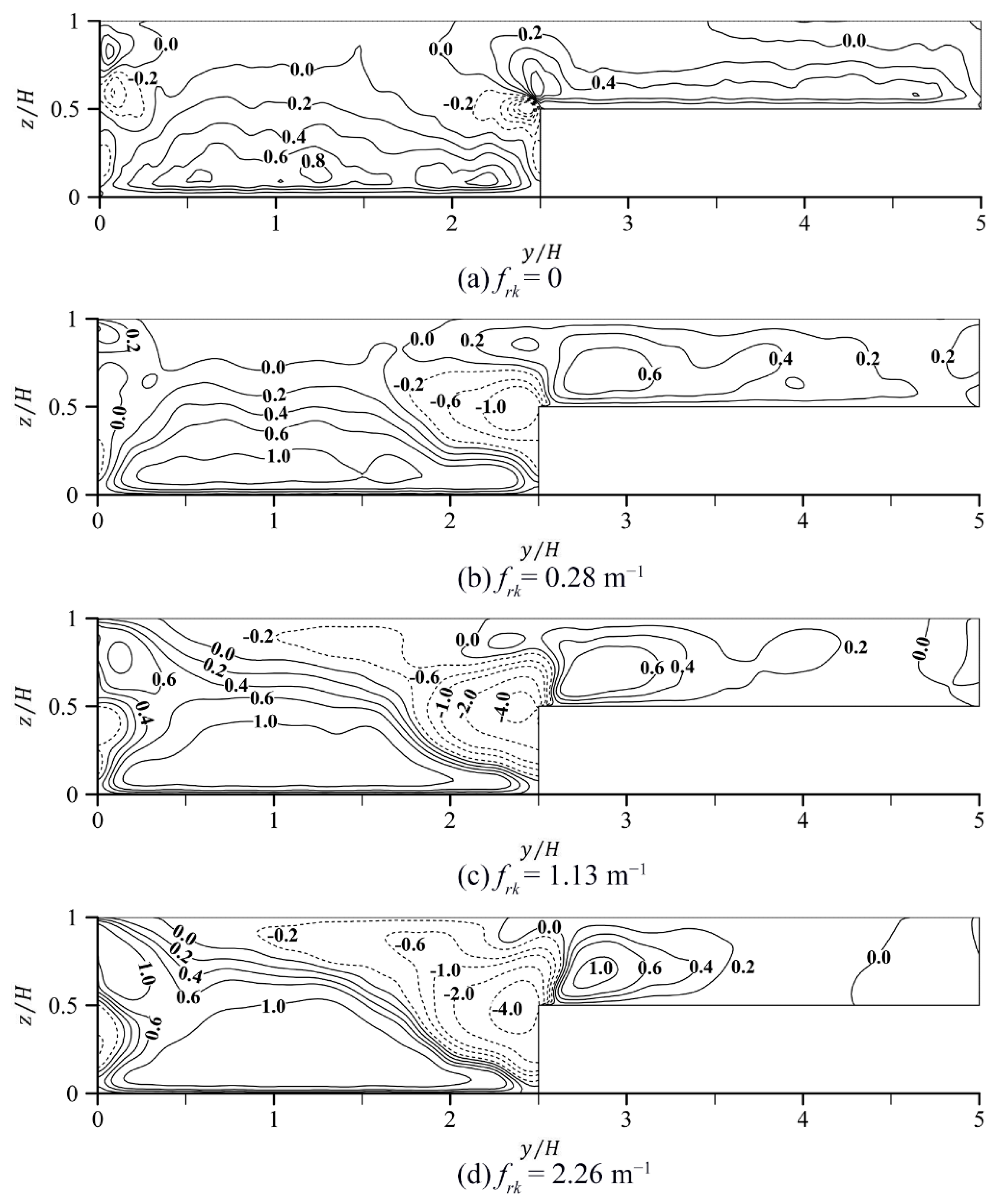
Figure 10 shows the dimensionless Reynolds stress with four different floodplain vegetation densities. As the vegetation density increased, the negative area of the Reynolds stress became larger. When the resistance parameter frk was 1.13 m−1 and 2.26 m−1, the negative area reached the water surface, while the value of the Reynolds stress near the bed gradually increased in the main channel. The computational results indicated that, when the floodplain roughened with vegetation, the exchange of mass and momentum was still the strongest near the interface of the main channel and floodplain. The Reynolds stress and the turbulence increased with the increase of floodplain vegetation density. When the floodplain was roughened with vegetation, increase of vegetation density did not result in any significant change in the Reynolds stress value near the side wall of the floodplain.
5.4. Lateral Momentum Exchange
The depth-averaged analysis of the streamwise momentum equation, facilitated analysis of the influence of floodplain vegetation on the transverse momentum exchange within compound open channel flows. Nezu and Onisuka [36] gave the depth-averaged streamwise momentum in open channel flows with vegetation as:
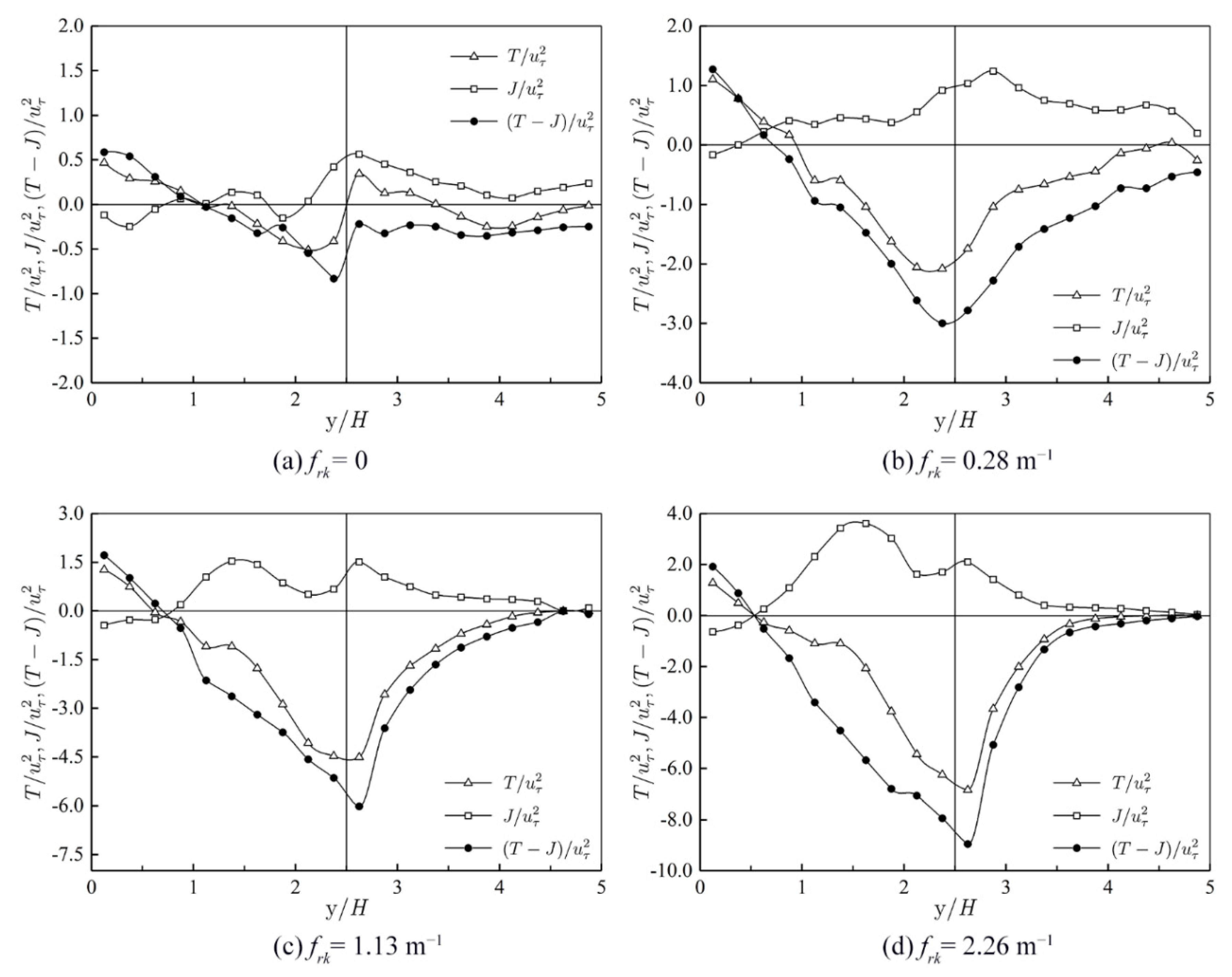
in which τb denotes the bed shear stress, its value corresponds to the total shear stress at z = 0; Ie denotes the energy gradient; h′ denotes the water depth; T denotes the shear stress induced by the Reynolds stress ; J denotes the shear stress induced by the secondary flow; (T-J) is the apparent shear stress, which quantitatively estimates the magnitude of the lateral transport of momentum.
The apparent shear stress (T-J), Reynolds stress component T and secondary currents component J with the four floodplain vegetation densities are shown in Figure 11. When the floodplain was vegetated, it can be seen that the absolute value of the shear stress T, J and the apparent shear stress (T-J) increased significantly. It is worth noting that the T, J, and T-J were almost the same near the side wall of the main channel for the four cases with different floodplain vegetation densities, indicating that floodplain vegetation had almost no effect on the vicinity of the side wall in the main channel. As the vegetation density increased, the total apparent shear stress reached a negative peak near the junction of the main channel and floodplain. The peak value became larger with increase of vegetation density. The intensity of secondary flow in the main channel and floodplain was gradually increasing, but its peak value shifted from the floodplain to the main channel. When the resistance parameter frk was 1.13 m−1 and 2.26 m−1, two peak values appeared in the secondary current component J.
Compared to the cases without floodplain vegetation, the transverse momentum exchange near the interface area, as well as that within the floodplain area, were found to be enhanced. The momentum exchange became more intensive, while the vegetation density increased. The contribution of the transverse turbulence to the momentum transport on the vicinity of the side wall in the main channel was almost unchanged. When y/H > 1, the momentum exchange of the secondary currents increased. The contribution of secondary currents on the momentum exchange became larger, while the vegetation density increased. However, the contribution of the lateral turbulence was still predominant in the momentum transport.
5.5. Vertical Structures
The Q-criterion, a popular method to define and identify the vortex structure in turbulent flows [37], was used in the analysis of vertical structure in the present study. The Q-value could be obtained as follows
in which and are the rotation rate tensor and strain rate tensor for the velocity gradients, respectively.
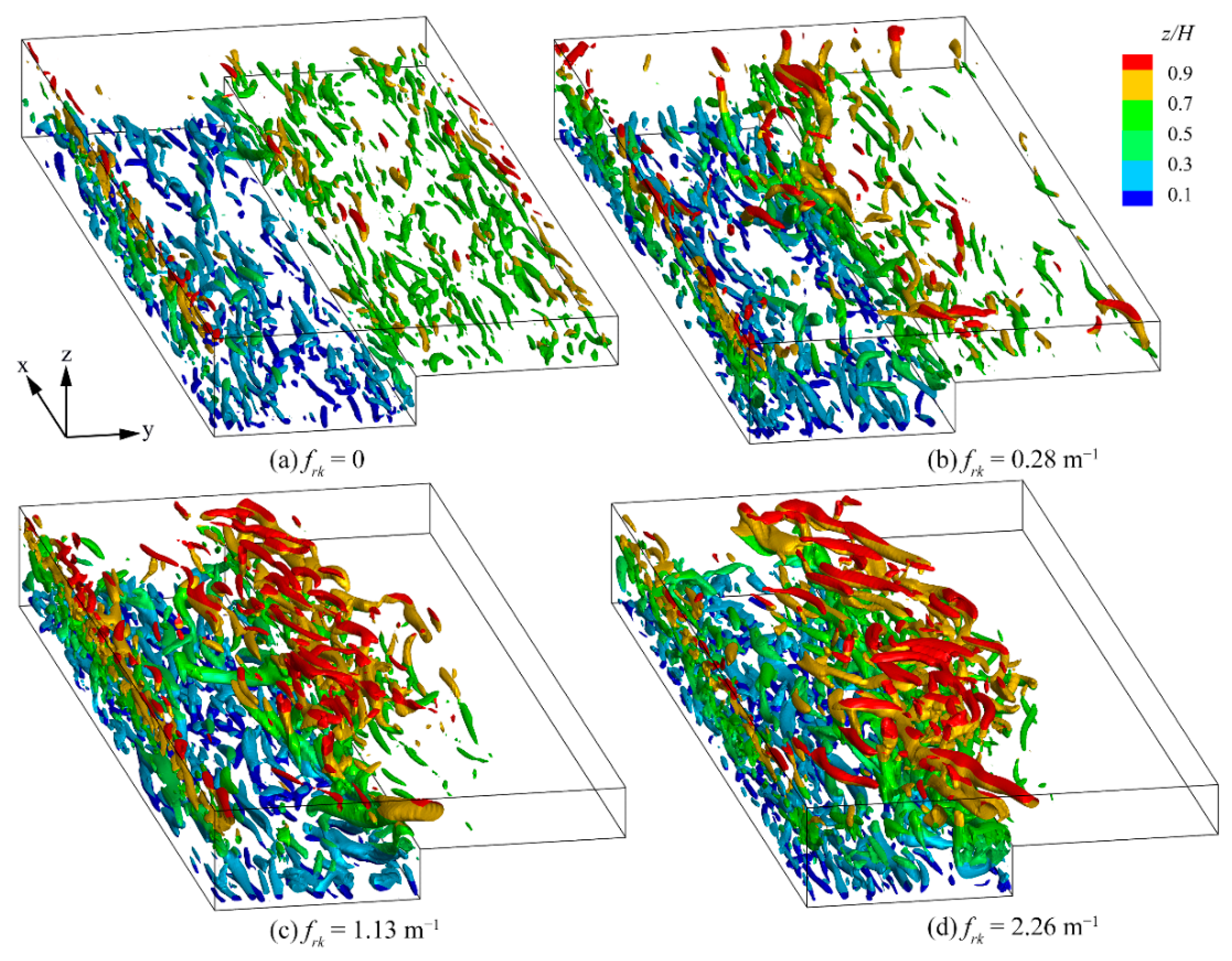
Figure 12 shows the instantaneous turbulent structures with four different floodplain vegetation densities obtained by using the Q criterion. The vortex structures were colored with the vertical dimensionless height (z/H). The threshold value of Q was set to be 50 in the present analysis. It can be seen from the figure that, when the vegetation density increased, the vortex structures on the floodplain gradually decreased, and the strip structures within the main channel increased. The strip structures were mainly concentrated near the interface of the main channel and floodplain, which was consistent with the time-averaged flow field. When the vegetation density was larger, there were a lot of strip structures close to the water surface at the junction area of compound open channel flows. The strip structure increased with the increase of vegetation density. This indicated that there was a strong horizontal shear layer near the side wall of the main channel and the junction area, resulting in the horizontal Kelvin–Helmholtz (K-H) coherent vortices. The K–H vortices enhanced the mixing of the flow in the horizontal direction. It is worth noting that the turbulence at the junction area was stronger. This also showed that, when the resistance parameter frk was 1.13 m−1 and 2.26 m−1, the strip structure in the floodplain significantly reduced. It was found that when the Q value was constant, more strip structures were captured in the main channel and less strip structures were observed in the floodplain while the floodplain was roughened with vegetation.
6. Conclusions
In this paper, WMLES simulations were performed for compound open channel flows with different floodplain vegetation densities. The vegetation-induced resistance effect was modeled with the drag force method, which was verified against experimental measurements and an analytical solution. Numerical simulations were conducted with four different vegetation densities (frk = 0, 0.28 m−1, 1.13 m−1 and 2.26 m−1). The LES results confirmed the findings of existing studies. The impact of vegetation density on flow field and turbulent structure was investigated and summarized. The following conclusions could be drawn.
Due to the vegetation-induced resistance effect, the flow velocity decreases within the floodplain and increases within the main channel, resulting in an increase in the bed shear stress within the main channel and a decrease in bed shear stress within the floodplain. When the floodplain vegetation density increases, the bed shear stress decreases in the floodplain and increases in the main channel. As the velocity gradient increases near the junction area, the bed shear stress changes more sharply.
Compared to the case without floodplain vegetation, the transverse turbulence of the water flow within the vicinity of the junction and in the floodplain increases, and is strengthened when floodplain vegetation density increases. Within the main channel, the impacts of the transverse turbulence on the momentum exchange near the vicinity of the side wall is almost unchanged. The strip structures are mainly concentrated near the interface area. The characteristics of instantaneous turbulent structure is consistent with that of the mean flow field. When the floodplain vegetation increases, strip structures within the floodplain decrease while the strip structures in the main channel increase.
Author Contributions
Conceptualization, C.Z. and J.Z.; methodology, F.Q. and S.D.; software, Y.B. and F.Q.; validation, J.Z. and S.D.; formal analysis, F.Q. and Y.H.; investigation, C.Z. and J.Z.; resources, C.Z.; data curation, S.D.; writing—original draft preparation, S.D.; writing—review and editing, C.Z. and J.Z.; visualization, Y.B. and Y.H.; supervision, C.Z.; project administration, C.Z.; funding acquisition, J.Z. and L.W. All authors have read and agreed to the published version of the manuscript.
Funding
This research was funded by the Fundamental Research Funds for the Central Universities (Grant No. B200202116, B200204044), National Key R&D Program of China (Grant No. 2022YFC3202605) and the 111 Project (Grant No. B17015).
Data Availability Statement
Not applicable.
Conflicts of Interest
The authors declare no conflict of interest.
References
- Yuan, S.; Xu, L.; Tang, H.; Xiao, Y.; Gualtieri, C. The dynamics of river confluences and their effects on the ecology of aquatic environment: A review. J. Hydrodyn. 2022, 34, 1–14. [Google Scholar] [CrossRef]
- Salauddin, M.; O’Sullivan, J.J.; Abolfathi, S.; Pearson, J.M. Eco-engineering of seawalls-an opportunity for enhanced climate resilience from increased topographic complexity. Front. Mar. Sci. 2021, 8, 674630. [Google Scholar] [CrossRef]
- O’Sullivan, J.; Salauddin, M.; Abolfathi, S.; Pearson, J.M. Effectiveness of eco-retrofits in reducing wave overtopping on seawalls. Coast. Eng. Proc. 2020, 36v, 13. [Google Scholar] [CrossRef]
- Liu, N.; Salauddin, M.; Yeganeh-Bakhtiari, A.; Pearson, J.; Abolfathi, S. The impact of eco-retrofitting on coastal resilience enhancement—A physical modelling study. IOP Conf. Ser. Earth Environ. Sci. 2022, 1072, 012005. [Google Scholar] [CrossRef]
- Naot, D.; Nezu, I.; Nakagawa, H. Hydrodynamic behavior of partly vegetated open channels. J. Hydraul. Eng. 1996, 122, 625–633. [Google Scholar] [CrossRef]
- Kang, H.; Choi, S.U. Turbulence modeling of compound open-channel flows with and without vegetation on the floodplain using the Reynolds stress model. Adv. Water. Resour. 2006, 29, 1650–1664. [Google Scholar] [CrossRef]
- Yang, K.J.; Liu, X.N.; Cao, S.Y.; Zhang, Z.X. Turbulence characteristics of overbank flow in compound river channel with vegetated floodplain. J. Theor. Appl. Mech. 2006, 38, 246–250. (In Chinese) [Google Scholar]
- Zhang, M.L.; Shen, Y.M.; Zhu, L.Y. Depth-averaged two-dimensional numerical simulation for curved open channels with vegetation. J. Hydraul. Eng. 2008, 39, 794–800. (In Chinese) [Google Scholar]
- Cui, J.; Neary, V.S. LES study of turbulent flows with submerged vegetation. J. Hydraul. Res. 2008, 46, 307–316. [Google Scholar] [CrossRef]
- Sun, X.; Shiono, K. Flow resistance of one-line emergent vegetation along the floodplain edge of a compound open channel. Adv. Water Resour. 2009, 32, 430–438. [Google Scholar] [CrossRef]
- Huai, W.X.; Gao, M.; Zeng, Y.H.; Li, D. Two-dimensional analytical solution for compound channel flows with vegetated floodplains. Appl. Math. Mech. 2009, 30, 1049–1056. [Google Scholar] [CrossRef]
- Zhang, M.L.; Li, C.W.; Shen, Y.M. A 3D non-linear k-ε turbulent model for prediction of flow and mass transport in channel with vegetation. Appl. Math. Model. 2010, 34, 1021–1031. [Google Scholar] [CrossRef]
- Zhang, M.W. Research on Flow Characteristics in Compound Channels with Vegetated Floodplains. Ph.D. Thesis, Tsinghua University, Beijing, China, 2011. (In Chinese). [Google Scholar]
- Zeng, C.; Li, C.W. Measurements and modeling of open-channel flows with finite semi-rigid vegetation patches. Environ. Fluid Mech. 2014, 14, 113–134. [Google Scholar] [CrossRef]
- Zeng, Y.H.; Huai, W.X.; Zhao, M.D. Flow characteristics of rectangular open channels with compound vegetation roughness. Appl. Math. Mech. 2016, 37, 341–348. [Google Scholar] [CrossRef]
- Dupuis, V.; Proust, S.; Berni, C.; Paquier, A. Mixing layer development in compound channel flows with submerged and emergent rigid vegetation over the floodplains. Exp. Fluids 2017, 58, 30. [Google Scholar] [CrossRef] [Green Version]
- Barman, J.; Kumar, B. Flow behaviour in a multi-layered vegetated floodplain region of a compound channel. Ecohydrology 2022, 15, e2427. [Google Scholar] [CrossRef]
- Paquier, A.; Oudart, T.; Bouteiller, C.L.; Meulé, S.; Larroudé, P.; Dalrymple, R.A. 3D numerical simulation of seagrass movement under waves and currents with GPUSPH. Int. J. Sediment Res. 2021, 36, 711–722. [Google Scholar] [CrossRef]
- Kazemi, E.; Koll, K.; Tait, S.; Shao, S.D. SPH modelling of turbulent open channel flow over and within natural gravel beds with rough interfacial boundaries. Adv. Water Resour. 2020, 140, 103557. [Google Scholar] [CrossRef]
- Donnelly, J.; Abolfathi, S.; Pearson, J.; Chatrabgoun, O.; Daneshkhah, A. Gaussian process emulation of spatio-temporal outputs of 2D inland flood model. Water Res. 2022, 225, 119100. [Google Scholar] [CrossRef]
- Goodarzi, D.; Lari, K.S.; Khavasi, E.; Abolfathi, S. Large eddy simulation of turbidity currents in a narrow channel with different obstacle configurations. Sci. Rep. 2020, 10, 12814. [Google Scholar] [CrossRef]
- Zeng, C.; Ding, S.W.; Zhou, J.; Wang, L.L.; Chen, C. A three-dimensional numerical simulation based on WMLES for compound open-channel turbulent flows. Adv. Sci. Technol. Water Resour. 2020, 40, 17–22. (In Chinese) [Google Scholar]
- Cater, J.E.; Williams, J.J.R. Large eddy simulation of a long asymmetric compound open channel. J. Hydraul. Res. 2008, 46, 445–453. [Google Scholar] [CrossRef]
- Xie, Z.H.; Lin, B.L.; Falconer, R.A. Large-eddy simulation of the turbulent structure in compound open-channel flows. Adv. Water Resour. 2013, 53, 66–75. [Google Scholar] [CrossRef]
- Ding, S.W.; Zeng, C.; Zhou, J.; Wang, L.L.; Chen, C. Impact of the depth ratio on the flow structure and turbulence characteristics of the compound open-channel flows. Water Sci. Eng. 2022, 15, 265–272. [Google Scholar] [CrossRef]
- Zeng, C.; Qiu, F.; Ding, S.; Zhou, J.; Xu, J.; Wang, L.; Yin, Y. Study on energy and momentum correction coefficients in compound open-channel flows. Hydro-Sci. Eng. 2022, 46–54. (In Chinese) [Google Scholar] [CrossRef]
- Dunn, C.; Lopez, F.; Garcia, M.H. Mean Flow and Turbulence in a Laboratory Channel with Simulated Vegetation. Available online: https://www.ideals.illinois.edu/items/12292 (accessed on 1 October 1996).
- Thomas, T.G.; Williams, J.J.R. Large eddy simulation of turbulent flow in an asymmetric compound channel. J. Hydraul. Res. 1995, 33, 27–41. [Google Scholar] [CrossRef]
- Canuto, C.; Hussaini, M.Y.; Quarteroni, A.; Zang, T. Spectral Methods in Fluid Dynamics; Springer: Amsterdam, The Netherlands, 1987. [Google Scholar]
- Shishkin, A.; Wagner, C. Direct Numerical Simulation of a Turbulent Flow Using a Spectral/hp Element Method. In New Results in Numerical and Experimental Fluid Mechanics V. Notes on Numerical Fluid Mechanics and Multidisciplinary Design (NNFM); Rath, H.J., Holze, C., Heinemann, H.J., Henke, R., Hönlinger, H., Eds.; Springer: Berlin/Heidelberg, Germany, 2006. [Google Scholar] [CrossRef]
- Rai, N.; Mondal, S. Spectral methods to solve nonlinear problems: A review. Partial. Differ. Equ. Appl. Math. 2021, 4, 100043. [Google Scholar] [CrossRef]
- Armanini, A. Roughness in fixed-bed streams. In Principles of River Hydraulics; Springer: Cham, Switzerland, 2018; pp. 1–31. [Google Scholar] [CrossRef]
- Kouwen, N. Modern approach to design of grassed channels. J. Irrig. Drain. Eng. 1992, 118, 733–743. [Google Scholar] [CrossRef]
- Huai, W.X.; Zeng, Y.H.; Xu, Z.G.; Yang, Z.H. Three-layer model for vertical velocity distribution in open channel flow with submerged rigid vegetation. Adv. Water Resour. 2009, 32, 487–492. [Google Scholar] [CrossRef]
- Righetti, M.; Armanini, A. Flow resistance in open channel flows with sparsely distributed bushes. J. Hydrol. 2002, 269, 55–64. [Google Scholar] [CrossRef]
- Nezu, I.; Onisuka, K. Turbulent structures in partly vegetated open-channel flows with LDA and PI V measurements. J. Hydraul. Res. 2001, 39, 629–642. [Google Scholar] [CrossRef]
- Hunt, J.C.R.; Wray, A.A.; Moin, P. Eddies, Stream, and Convergence Zones in Turbulent Flows; Center for Turbulence Research Report: Stanford, CA, USA, 1988; pp. 193–208. [Google Scholar]
Figure 1.
Resistance effect induced by vegetation.

Figure 2.
Schematic diagram of longitudinal section of simulation area.

Figure 3.
Comparison of the time-averaged dimensionless streamwise flow velocity.

Figure 4.
Comparison of dimensionless fluctuating flow velocity.

Figure 5.
Comparison of dimensionless Reynolds stress.

Figure 6.
Schematic diagram of the compound open channel flows with floodplain vegetation.

Figure 7.
Sectional distribution of streamwise velocity U and secondary currents (V, W) with different floodplain vegetation densities. (a) Case with frk = 0. (b) Case with frk = 0.28 m−1. (c) Case with frk = 1.13 m−1. (d) Case with frk = 2.26 m−1.
Figure 7.
Sectional distribution of streamwise velocity U and secondary currents (V, W) with different floodplain vegetation densities. (a) Case with frk = 0. (b) Case with frk = 0.28 m−1. (c) Case with frk = 1.13 m−1. (d) Case with frk = 2.26 m−1.

Figure 8.
Bed shear stress with different floodplain vegetation densities.

Figure 9.
Reynolds stress with different floodplain vegetation densities. (a) Case with frk = 0. (b) Case with frk = 0.28 m−1. (c) Case with frk = 1.13 m−1. (d) Case with frk = 2.26 m−1.
Figure 9.
Reynolds stress with different floodplain vegetation densities. (a) Case with frk = 0. (b) Case with frk = 0.28 m−1. (c) Case with frk = 1.13 m−1. (d) Case with frk = 2.26 m−1.

Figure 10.
Reynolds stress with different floodplain vegetation densities. (a) Case with frk = 0. (b) Case with frk = 0.28 m−1. (c) Case with frk = 1.13 m−1. (d) Case with frk = 2.26 m−1.
Figure 10.
Reynolds stress with different floodplain vegetation densities. (a) Case with frk = 0. (b) Case with frk = 0.28 m−1. (c) Case with frk = 1.13 m−1. (d) Case with frk = 2.26 m−1.

Figure 11.
The apparent shear stress distribution with different floodplain vegetation densities. (a) Case with frk = 0. (b) Case with frk = 0.28 m−1. (c) Case with frk = 1.13 m−1. (d) Case with frk = 2.26 m−1.
Figure 11.
The apparent shear stress distribution with different floodplain vegetation densities. (a) Case with frk = 0. (b) Case with frk = 0.28 m−1. (c) Case with frk = 1.13 m−1. (d) Case with frk = 2.26 m−1.

Figure 12.
Instantaneous turbulent structure with different floodplain vegetation densities. (a) Case with frk = 0. (b) Case with frk = 0.28 m−1. (c) Case with frk = 1.13 m−1. (d) Case with frk = 2.26 m−1.
Figure 12.
Instantaneous turbulent structure with different floodplain vegetation densities. (a) Case with frk = 0. (b) Case with frk = 0.28 m−1. (c) Case with frk = 1.13 m−1. (d) Case with frk = 2.26 m−1.


Table 1.
Physical model parameters in Dunn et al. (1996).
| Q (m3/s) | H (m) | hv (m) | bv (m) | S0 | frk (m−1) |
|---|---|---|---|---|---|
| 0.179 | 0.335 | 0.1175 | 0.0064 | 0.0036 | 1.23 |
Publisher’s Note: MDPI stays neutral with regard to jurisdictional claims in published maps and institutional affiliations. |
© 2022 by the authors. Licensee MDPI, Basel, Switzerland. This article is an open access article distributed under the terms and conditions of the Creative Commons Attribution (CC BY) license (https://creativecommons.org/licenses/by/4.0/).
Share and Cite
MDPI and ACS Style
Zeng, C.; Bai, Y.; Zhou, J.; Qiu, F.; Ding, S.; Hu, Y.; Wang, L. Large Eddy Simulation of Compound Open Channel Flows with Floodplain Vegetation. Water 2022, 14, 3951. https://doi.org/10.3390/w14233951
AMA Style
Zeng C, Bai Y, Zhou J, Qiu F, Ding S, Hu Y, Wang L. Large Eddy Simulation of Compound Open Channel Flows with Floodplain Vegetation. Water. 2022; 14(23):3951. https://doi.org/10.3390/w14233951
Chicago/Turabian StyleZeng, Cheng, Yimo Bai, Jie Zhou, Fei Qiu, Shaowei Ding, Yudie Hu, and Lingling Wang. 2022. "Large Eddy Simulation of Compound Open Channel Flows with Floodplain Vegetation" Water 14, no. 23: 3951. https://doi.org/10.3390/w14233951
Note that from the first issue of 2016, this journal uses article numbers instead of page numbers. See further details here.