
Groundwater Modeling with Process-Based and Data-Driven Approaches in the Context of Climate Change
by
 ,
,
Matia Menichini
1 ,
,
Linda Franceschi
1,2,*,
Brunella Raco
1,
Giulio Masetti
1,
Andrea Scozzari
3 and
Marco Doveri
1 1
Istituto di Geoscienze e Georisorse-Consiglio Nazionale delle Ricerche (IGG-CNR), Via G. Moruzzi 1, 56124 Pisa, Italy
2
Dipartimento di Scienze della Terra, Università di Pisa, Via Santa Maria 53, 56126 Pisa, Italy
3
Istituto di Scienza e Tecnologie dell’Informazione-Consiglio Nazionale delle Ricerche (ISTI-CNR), Via G. Moruzzi 1, 56124 Pisa, Italy
*
Author to whom correspondence should be addressed.
Water 2022, 14(23), 3956; https://doi.org/10.3390/w14233956
Submission received: 5 October 2022
/
Revised: 23 November 2022
/
Accepted: 25 November 2022
/
Published: 5 December 2022
(This article belongs to the Special Issue Groundwater Hydrological Model Simulation)
Abstract
:In the context of climate change, the correct management of groundwater, which is strategic for meeting water needs, becomes essential. Groundwater modeling is particularly crucial for the sustainable and efficient management of groundwater. This manuscript provides different types of modeling according to data availability and features of three porous aquifer systems in Italy (Empoli, Magra, and Brenta systems). The models calibrated on robust time series enabled the performing of forecast simulations capable of representing the quantitative and qualitative response to expected climate regimes. For the Empoli aquifer, the process-based models highlighted the system’s ability to mitigate the effects of dry climate conditions thanks to its storage capability. The data-driven models concerning the Brenta foothill aquifer pointed out the high sensitivity of the system to climate extremes, thus suggesting the need for specific water management actions. The integrated data-driven/process-based approach developed for the Magra Valley aquifer remarked that the water quantity and quality effects are tied to certain boundary conditions over dry climate periods. This work shows that, for groundwater modeling, the choice of the suitable approach is mandatory, and it mainly depends on the specific aquifer features that result in different ways to be sensitive to climate. This manuscript also provides a novel outcome involving the integrated approach wherein it is a very efficient tool for forecasting modeling when boundary conditions, which significantly affect the behavior of such systems, are subjected to evolve under expected climate scenarios.
1. Introduction
Most of the available freshwater sources on Earth are stored underground; therefore, groundwater represents the main source of water supply [1]. Worldwide, more than 2 billion people depend on groundwater for their daily water use [2]. In many areas, groundwater bodies represent the most important and safest source of drinking water [3,4]. In European countries, for example, groundwater exploitation provides water for human consumption for 70% of the population on average [5]. Groundwater withdrawals supply 40% of industrial water [6], and groundwater use for irrigation is also significant and increasing. Siebert et al. [7] estimated that, globally, 38% of the area equipped for irrigation is provided by groundwater.
The reliance on this resource is continuously growing [8], given the key role that groundwater plays in mitigating climate change/variability and in addressing the significant increase in the global water demand, which has been predicted as a consequence of the future economic expansion, population growth, and urbanization [1,9].
Both present observations and simulations of climate conditions point out that changes are occurring or will occur in several regions in terms of higher temperatures, lower precipitation, increases in climatic extremes, and climate types [10,11,12,13,14]. Although groundwater systems are more resilient to climate change than surface waters, they are affected both directly and indirectly [15,16], especially when referring to local groundwater flow with low travel time [17].
Despite this, and unlike surface waters, groundwater bodies have not been widely studied, and there is a general paucity of quantitative information, especially in relation to climate change. The estimation of the entity of these effects is mandatory for the reliable management of this crucial resource, which must be protected by suitable actions in order to guarantee a safe water supply for the next generations [18].
Groundwater modeling is particularly crucial for the sustainable and efficient management of groundwater resources, even more in the context of expected climate change. Process-based or empirical (data-driven) numerical models can be used to model groundwater.
For the implementation of process-based models, it is necessary to know the boundary conditions, hydrogeological variables, and structural complexities of the aquifers [19]; in other words, it is necessary to know the conceptual model that is the synthesis of what is known and quantified on the system [20]. These models use deterministic and spatially distributed data, which must be characterized by significant accuracy. Their application to heterogeneous aquifers and particular situations within the hydrogeological domain (e.g., groundwater–river interactions) can lead to significant uncertainty associated with the number and complexity of parameters, as well as with the type of modeling itself based on the head-oriented approach (HOA) [21,22]. In such cases, aside from the alternative of the MODFLOW-based velocity-oriented approach (VOA) [22], an additional possible approach is to use the stochastic approach in defining the aquifer parameters [23].
In contrast, data-driven models involve mathematical equations that are not derived from prior knowledge of the physical process. Rather, they are based on the analysis of input/output relationships in the process under observation [24,25,26], even if the knowledge of the general conceptual model of the systems can significantly steer the development of the data-driven approach. To perform such analysis, mathematical tools, often involving machine-learning techniques, are used to approximate the behavior of the physical process on the basis of available datasets that describe its input/output transfer functions (e.g., linear regressions, multilinear regressions, neural network models, etc.). Therefore, data-driven models can be efficiently used to describe particular and specific processes [27,28] that are hard to determine with a physically based approach and can eventually be incorporated into larger physically based models [29,30,31].
Generally, process-based models are preferred over data-driven models because the first can make acceptable forecasts when a large number of observations are not available and when future conditions lie outside the range of stresses in the historical record, such as responses to climate change [19]. Moreover, the data-driven approach has the limitation of referring to punctual situations or specific processes in the groundwater system (e.g., relationships between superficial water and groundwater) and not to the entire volume or significant portions of the aquifer, as in the case of process-based models. Additionally, for this reason, the latter is generally preferred by decision-makers to steer groundwater management actions.
This manuscript provides different experiences of groundwater modeling applied to porous aquifer systems, with the aim of emphasizing the criteria of the methodology choice, its advantages and disadvantages, and the potentiality of a combined approach.
All the presented models represent operational tools for the reliable management of the water resource, as well as diagnostic tools to understand the functioning of the aquifer system better and how the effects of climate change in the short and long term affect the water resource quantity and quality.
2. Materials and Methods
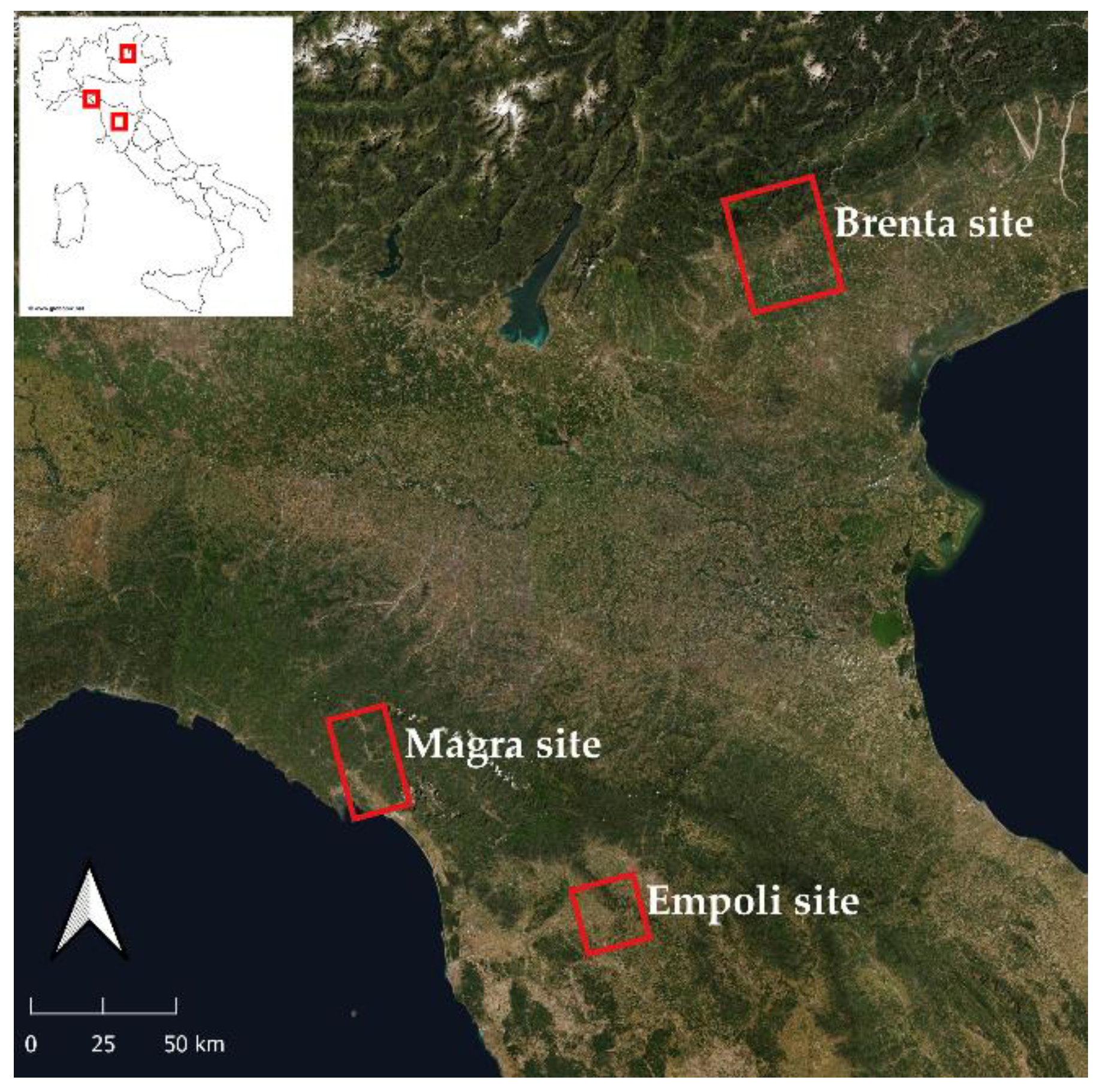
Three case studies are presented (Figure 1): the Empoli plain aquifer system, which was modeled using a process-based model; the foothill aquifer system of the Brenta River plain, where a mathematical regression model was applied; and the Magra Valley aquifer system, where a combined approach with process-based and data-driven modeling was developed.
The considered case studies encompass different combinations of recharge mechanisms, thus providing cases with different implications of climate change for groundwater systems [32]. Particularly, we analyzed situations in which the diffuse recharge is dominant and situations in which the focused recharge (i.e., losing rivers) is from significant to principal and, therefore, very sensitive to changes in the weather and climate regime, both in terms of quantity availability and water quality [33].
The first step was to collect data on meteo-climatic parameters, geology, hydrogeology, geochemistry and isotope signatures, as well as on the main items entering or leaving the system (e.g., well withdrawal). All the data collected were processed and compared in order to define a conceptual model that summarizes and quantifies the main processes and constraints of the aquifer for the purpose of developing the mathematical model.
Most geological, hydrogeological, and geochemical information used to elaborate the conceptual model of the different areas derive from the numerous studies that the authors carried out in cooperation with local authorities (Tuscany Region, Water Authorities, Water Managers) and/or in the frame of doctoral theses.
As a consequence of the hydrogeological and hydrodynamic features of the systems and data availability, different types of mathematical modeling were chosen: process-based modeling, data-driven modeling, and a combined approach.
2.1. Process-Based Model
The process-based model uses processes and principles of physics to represent flow, and it consists of: (i) a governing equation that describes the physical process within the problem domain; (ii) boundary conditions that specify heads or flow along the boundaries; and (iii) for time-dependent problems, initial conditions that specify head at the beginning of the simulation [19]. Groundwater flow models can be solved analytically or numerically for the distribution of heads in space and in time for transient problems. Assumptions built into analytical solutions limit their application to relatively simple systems [34], and usually, they are inappropriate for real groundwater problems. Typically, numerical models based on finite differences are used to simulate groundwater flow.
In this work, the codes used to process the input data and solve the process-based equation that describes the groundwater system are MODFLOW [35] and related codes. Groundwater Vistas [36] and Groundwater Modeling Systems [37] were used as graphical user interfaces.
The model creation started with the implementation phase, where the domain in space and time was discretized, hydraulic parameters applied, and boundary conditions defined based on the conceptual model previously defined. Subsequently, the model was calibrated on the basis of a comparison between the simulated and collected data. The calibration was performed manually (trial-and-error method) and automatically using specific code, like the PEST code [38].
Once a sufficiently calibrated model was obtained, forecast simulations were then carried out with the aim of assessing how the expected extreme climatic regimes would affect the groundwater quantity and quality.
The development of this type of model requires a large amount of information and input data evenly distributed over the domain. In particular, it is necessary to know the geometries of the system under study, the hydraulic parameters of the various lithotypes that make it up and to identify and quantify the main components entering and leaving the system. Moreover, the representativeness of the model itself is inextricably linked to the availability and reliability of the data required in the calibration phase.
The process-based modeling was applied to a porous multilayer system (Empoli plain aquifer system) in the central part of the Arno River catchment (Central Italy, Tuscany) because previous knowledge and available data were deemed sufficient and suitable for the development of this type of model.
2.2. Data-Driven Model
Data-driven models use empirical or statistical equations derived from the available data to approximate the input/output relationships between physical variables characterizing a system without quantifying its process and physical properties [19].
Initially, a site-specific equation is developed by fitting parameters either empirically or statistically to reproduce the historical data (e.g., piezometric level) in response to other parameters (e.g., surface water level, precipitation). This equation is subsequently used to calculate the response to future stresses.
This type of modeling requires a large number of observations of heads that ideally encompass the range of all expected stresses to the system, but it is independent of the knowledge of numerous parameters distributed over the territory that is often difficult to find, as well as the hydrogeological processes taking place in the aquifer system. Data-driven models are very powerful, but they only estimate a given variable on one or more individual points and do not return information on a domain scale (e.g., water balance).
Considering the very long time series of numerous continuous monitoring stations of precipitation, hydrometric, and piezometric levels in the foothill aquifer system of the Brenta River (North-East Italy, Veneto), and pending a more detailed reconstruction of the hydro-structures, the first attempt of a mathematical regression model was developed for this system. In particular, a Multiple Linear Analysis (MLRA) was performed, considering dependent and independent variables; in this case, piezometric levels were estimated by means of hydrometric level and rainfall quantity.
Various regression models were carried out using transformation of the raw variable (e.g., moving average, shift) to maximize the correlation coefficient between the dependent and independent variables. The main steps of the workflow can be summarized as follows:
- (1)
- Gap filling;
- (2)
- Trend and outlier analysis;
- (3)
- Autocorrelation and cross-correlation;
- (4)
- MLRA;
- (5)
- Residual analysis;
- (6)
- Validation and forecasting.
All of these procedures were applied by selecting one piezometer and one hydrometric station that are representative of the main hydrological process occurring in the Brenta aquifer system, consisting of the groundwater–streamwater exchanges.
2.3. Process-Based and Data-Driven Models Combined
To develop a predictive flow and transport process-based model in order to evaluate the behavior of the aquifer in anticipated climate scenarios, it is often necessary to implement the value of expected precipitation plus expected values for additional constraints that are strongly related to the rainfall itself, such as river levels or heads of boundary conditions. This is particularly important in the systems where the groundwater flow response is deeply affected by such local constraints (e.g., losing a river whose feeding rate is relevant to the total water budget of the aquifer system) in comparison with the effects of diffuse rainwater infiltration. In order to address these issues, a possible solution is to realize a data-driven model able to reproduce over time boundary conditions (e.g., rivers and constant head or general head boundaries) of the physical model under hypothetic (or “synthetic”) future climate scenarios.
The production of synthetic scenarios is a fundamental step in this type of approach, as it permits the analysis and evaluation of situations that are plausible but not necessarily recorded in historical data series. More in detail, the basic concept is to produce a synthetic time series inspired by historical series, to establish hypothetical but plausible trends of parameters that are insufficiently monitored or not monitored at all, and to thicken the statistical database used for training machine learning algorithms.
This type of combined approach, therefore, requires not only an appropriate knowledge of the aquifer system, as well as the availability of reliable data appropriately distributed throughout the territory for correct implementation and calibration of the process-based numerical model, but also the availability of robust data sets on strategic continuous monitoring points for the development of data-driven models.
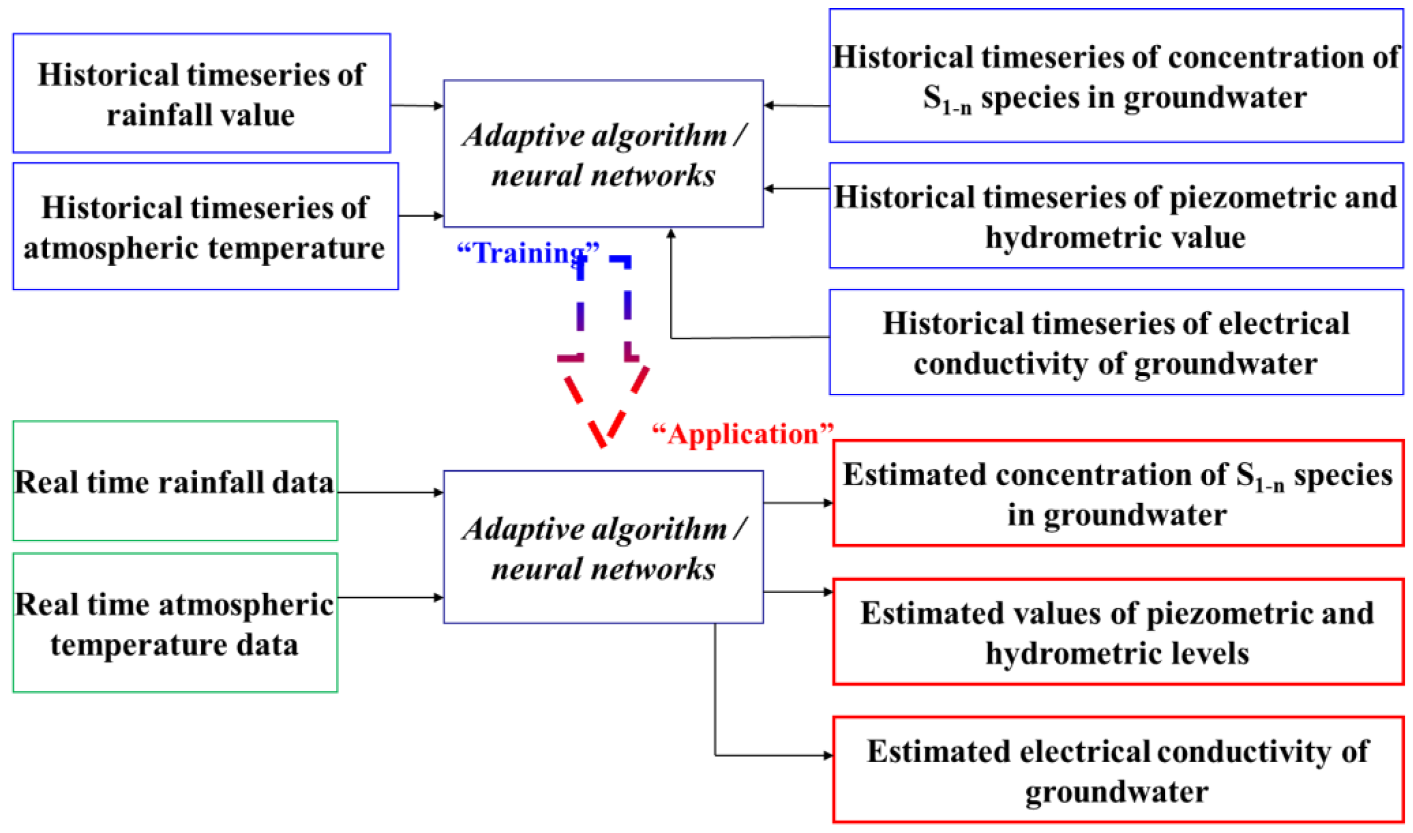
The aquifer system of the Magra River plain (North-West Italy, Liguria) was taken as a case study for this type of approach due to the great number of measurement points and the availability of robust time series for significant boundary conditions. The first step was to create a suitably calibrated flow and transport process-based model. Subsequently, in order to create a useful dataset to implement the boundary conditions of the forecasting model, fully synthetic datasets were generated as a training set of the data-driven scheme, with input variables inspired by selected climate models and input/output relationships estimated by past observations (Figure 2). In particular, the rainfall time series was generated stochastically by means of the WeaGETS package [39], using as input the rainfall time series actually measured at a rain gauge located in the area of interest, whereas the synthetic time series of temperature was based on the MarkSim simulation system [40]. An experimental run of the flow-transport model for 30 years ahead was therefore performed based on such hypothetic scenarios.
3. Results
3.1. Process-Based Models of the Empoli Aquifer System
As previously mentioned, given the knowledge degree of the Empoli aquifer system and considering the available data, it was decided to develop process-based models in order to provide the water manager with a tool for planning a sustainable use of the resource under possible future weather and climate conditions.
3.1.1. Conceptual Model
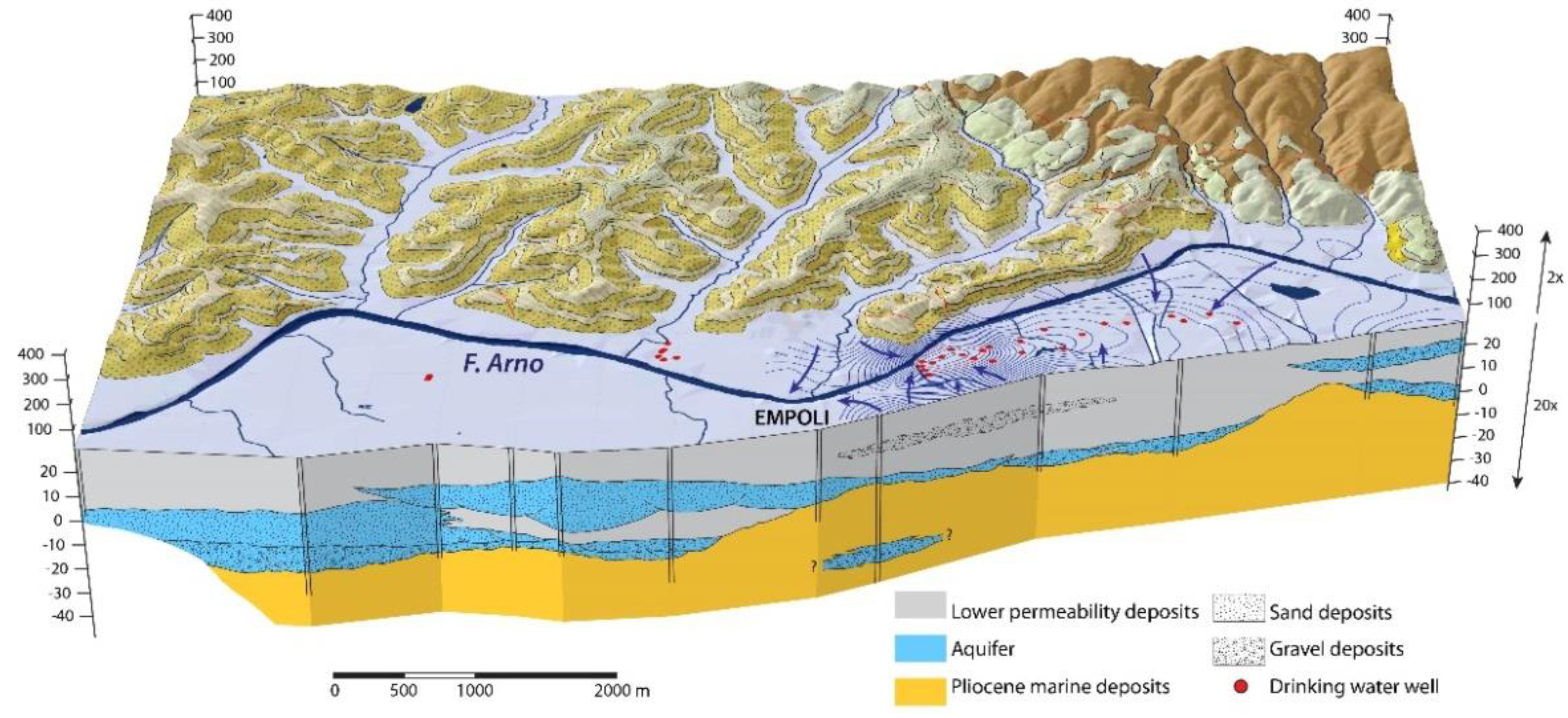
The Empoli aquifer system develops in the plain of the middle part of the River Arno catchment (Figure 3). From a geological point of view, the area corresponds to a wide depression filled by Neogene-Quaternary deposits and recent alluvium sediments that reaches a maximum thickness of around 40 m lying on a substratum of Pliocene marine deposits, mainly made up of clays. Overall, the aquifer system consists of two main permeable layers characterized by a significant lateral extension, to which lower permeability deposits are interbedded (Figure 3).
Based on the 3D reconstruction of the subsoil (Figure 3), it can be stated that:
- The chiefly confined lower aquifer layer consists of sandy gravels and gravels with an average thickness of approx. 7 m (maximum 14 m). The base of the aquifer is represented by the Pliocene substratum. This aquifer is separated from the upper aquifer by a clayey layer of variable thickness (average 7 m) and spatially discontinuous. Locally, where the clayey septum is not present, this aquifer level is hydraulically connected to the shallower one.
- The upper aquifer was reconstructed with continuity over the entire domain and represented the main aquifer in volumetric terms. It is composed of sand and gravel, often in mixed components; the grain size varies from predominantly gravelly sandy in the sectors facing the Arno River to a sandy loamy in the more distal areas. The average thickness of the aquifer is approx. 10 m, with varying values up to 20 m.
- Generally, a horizon defined in the reconstruction as an aquitard/aquiclude is above the most superficial aquifer, but its grain composition, typically consisting of clayey and sandy silts, is such that it does not impart a purely confined character to the most superficial aquifer.
Based on hydraulic tests performed on a lot of drinkable wells in the Empoli area, transmissivity values characterizing the aquifer horizons vary between about 2 × 10⁻³ and 2 × 10⁻² m2/s and hydraulic permeability values between about 2 × 10⁻⁴ and 2 × 10⁻³ m/s, in accordance with the gravelly sandy grain sizes.
Based on previous multidisciplinary studies [41,42,43] that involved geological, hydrogeological, and isotopic-hydrochemistry elaborations, the recharge of the system is mainly from direct infiltration. Furthermore, there are significant contributions from rivers (in particular from the Arno and Pesa rivers), as well as secondary underground transfers from the hill system along the foothill margins. As regards meteoric recharge, on the basis of historical data [44], it is possible to calculate an average annual value (data from 2000 to 2018) of 776 mm of rainfall and an average evapotranspiration value of 456 mm with an effective rainfall value of 320 mm [45]. The main outflows from the system are wells withdrawal, the drainage action of the Arno River in limited sectors, and natural underground outflowing of the modeled domain at the west. As far as outflows are concerned, the wells have been subdivided according to the use (domestic, agricultural, industrial, drinkable use) on the basis of available information and land use. For wells of drinking water supply, the consumptions were provided by Acque SpA (average annual flow rates for the period 2011–2016; average monthly flow rates for 2017), whereas for the wells used in agricultural and industrial activities, the pumping rates were estimated from a study of the Tuscan Region’s Hydrological Service [46]. Table 1 shows the estimated consumption for each type of use in the model domain.
3.1.2. Models Implementation
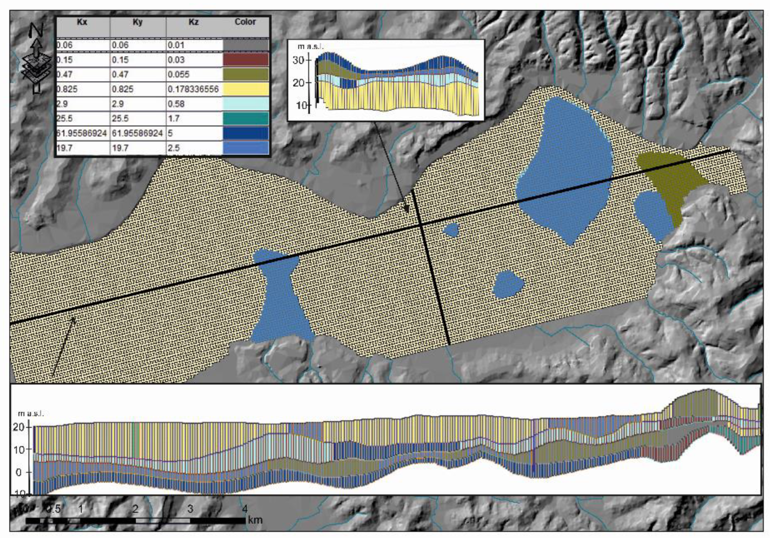
The model domain is shown in Figure 4. The space has been discretized by 108 rows and 291 columns with cells of 50 × 50 m and four layers for a total of 125,712 cells, of which 81,856 are active. The thickness of the cells varies according to the geometry of the geological model (Figure 4). Specifically, the first layer is mainly representative of the horizon defined in the reconstruction as an aquitard/aquiclude; the second and fourth layers are representative of the shallower and deeper aquifers, respectively; the third layer was implemented to represent the impermeable interlayer separating the two main aquifers when present. The assigned hydraulic conductivity is also shown in Figure 4.
From a temporal point of view, a steady-state model was initially implemented, thus taking into account the average values of all input data; subsequently, a transient-state model was implemented with monthly stress periods covering the period from January 2016 to December 2017.
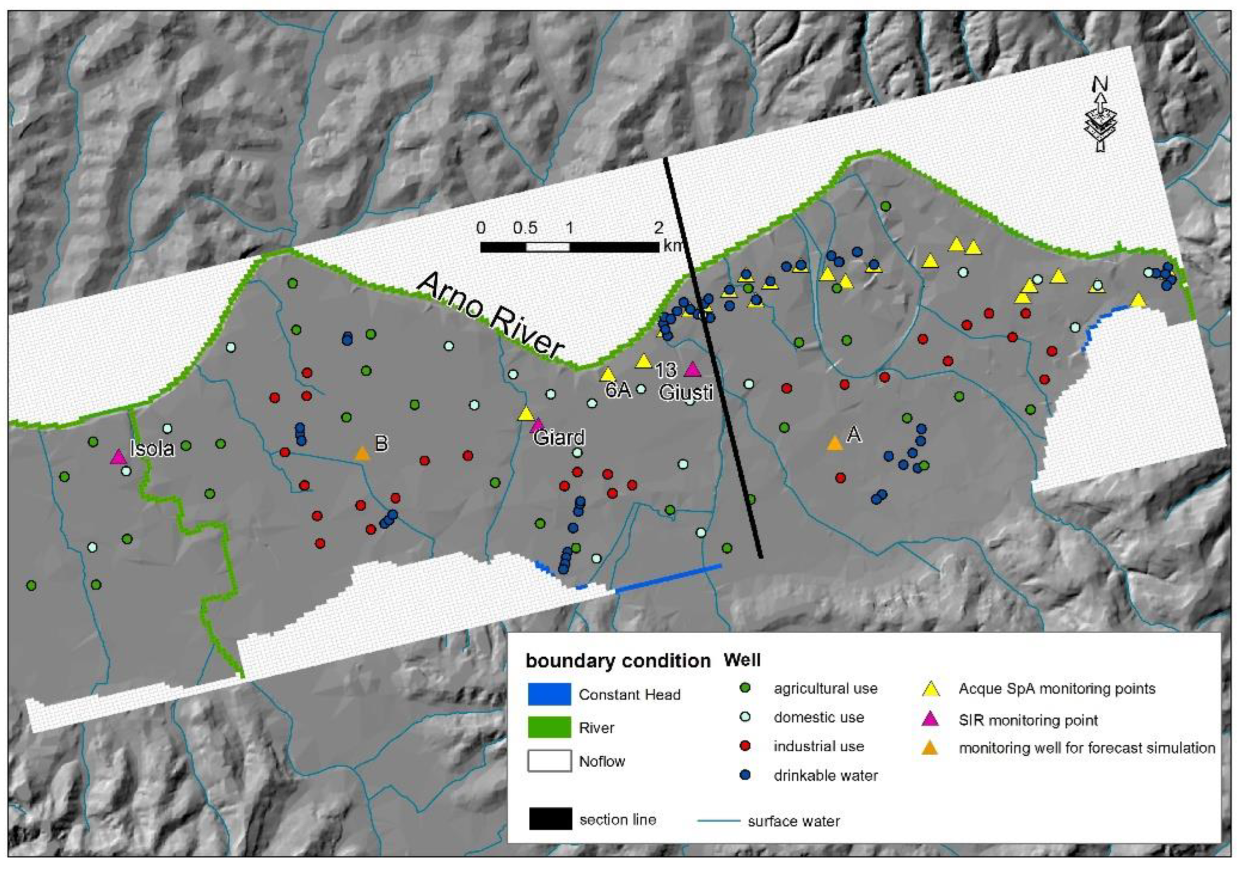
The main components entering or leaving the system were mathematically represented through boundary conditions (Figure 5). Boundary conditions of the first type (Constant Head) were set in those sectors (boundaries to the south) where previous studies [42,43] indicate a significant feed component, as well as in the boundary to the west of the model to represent the natural subterranean outflow through that sector (downstream zone). The values assigned to these boundaries were defined on the basis of available monitoring data and subsequently refined during the calibration phase.
The main watercourses were represented using a third type of boundary condition (River). The implemented water level data are derived from those recorded by monitoring stations in the area (data available online at www.sir.toscana.it, accessed on 1 March 2018), the river bed elevation and width data from Lidar images (data available online at http://www502.regione.toscana.it/geoscopio/cartoteca.html, accessed on 1 March 2018). For the permeability of the river bed sediments, a value between 0.86 and 8.64 m/d was set, whereas their thickness was arbitrarily set at 1 m.
The effective rainfall value (precipitation-evapotranspiration) was used and multiplied by an infiltration coefficient related to land use to represent the effective infiltration (0.25 in an urban environment and 0.4 in a rural environment). For the steady-state model, the average effective rainfall value calculated for the period (2000–2018) was used, and for the transient-state model, the monthly values were calculated.
The initial conditions of hydraulic loading in the aquifer were set equal to the ground level elevation for the steady-state simulation, while for the transient-state model, they correspond to the piezometric surface returned by the steady-state model.
3.1.3. Models Calibration, Validation, and Output
For the calibration of the models, the data of three stations belonging to the continuous monitoring network of the SIR were used (Isola, Giardino Val Gardena, and Via Giusti, respectively named Isola, Giard, and Giusti in Figure 5), as well as the piezometric levels measured on some monitoring points provided by Acque SpA (Figure 5), which perform a monitoring activity on a network defined as the ‘Empoli profile’.
For the steady-state model, the average values of all available data were used. For the transient-state model, on the other hand, monthly average values were calculated with the daily data of the SIR stations [44], while for the other points, the discrete measurement was attributed to the stress period in which it fell.
In conjunction with the calibration process, a sensitivity analysis was carried out in order to make the identification of those parameters whose changes have the greatest influence on the results of the simulations possible. Specifically, the most sensitive parameters were found to be the hydraulic conductivity of zone four and zone seven, representative of the surface semi-permeable horizon and the deep aquifer, respectively.
Following an initial coarser calibration using the trial-and-error method, the PEST code was subsequently used to better calibrate the model by varying the most sensitive parameters by no more than 10% compared to what was defined on the basis of the conceptual model.
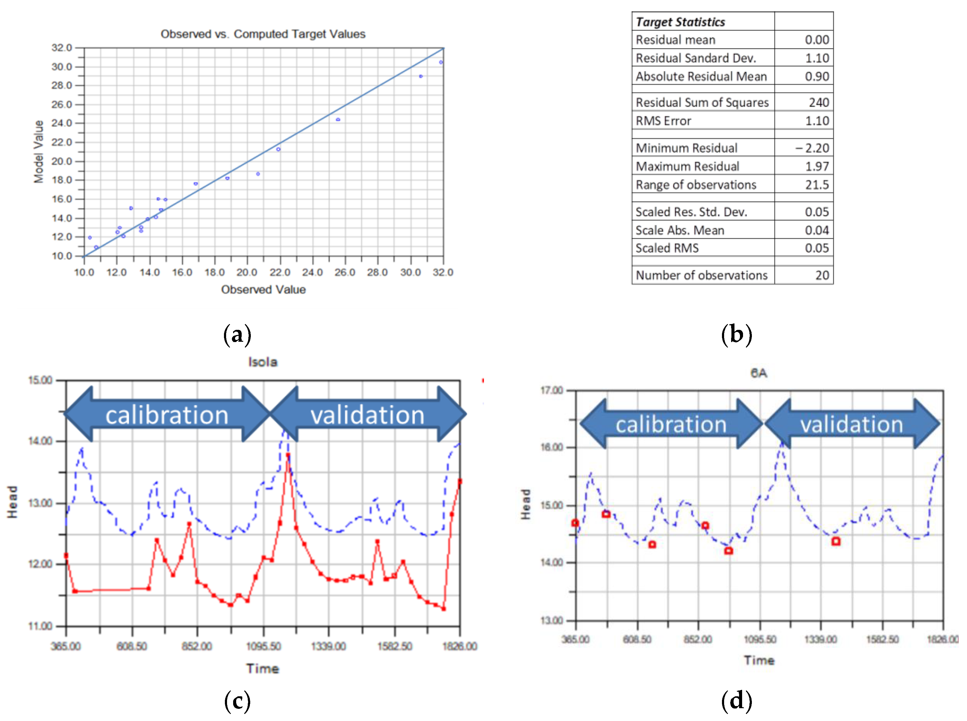
The results of the calibrated steady-state model are shown in Figure 6a,b, whereas in the diagrams of Figure 6c,d, it is possible to observe the variations over time of the experimental piezometric levels in comparison to the level evolution simulated with the transient-state model in selected monitoring points during the calibration and validation periods.
From the analysis of these diagrams (Figure 6), it can be observed that the model as a whole is sufficiently representative in terms of both absolute values and monthly trends, obviously in the areas where calibration targets are present. The modeled levels of the Isola target are very consistent in terms of evolution with respect to the experimental data. However, the residual values are significant (about 1 m), likely because of local conditions that do not allow knowing the available information.
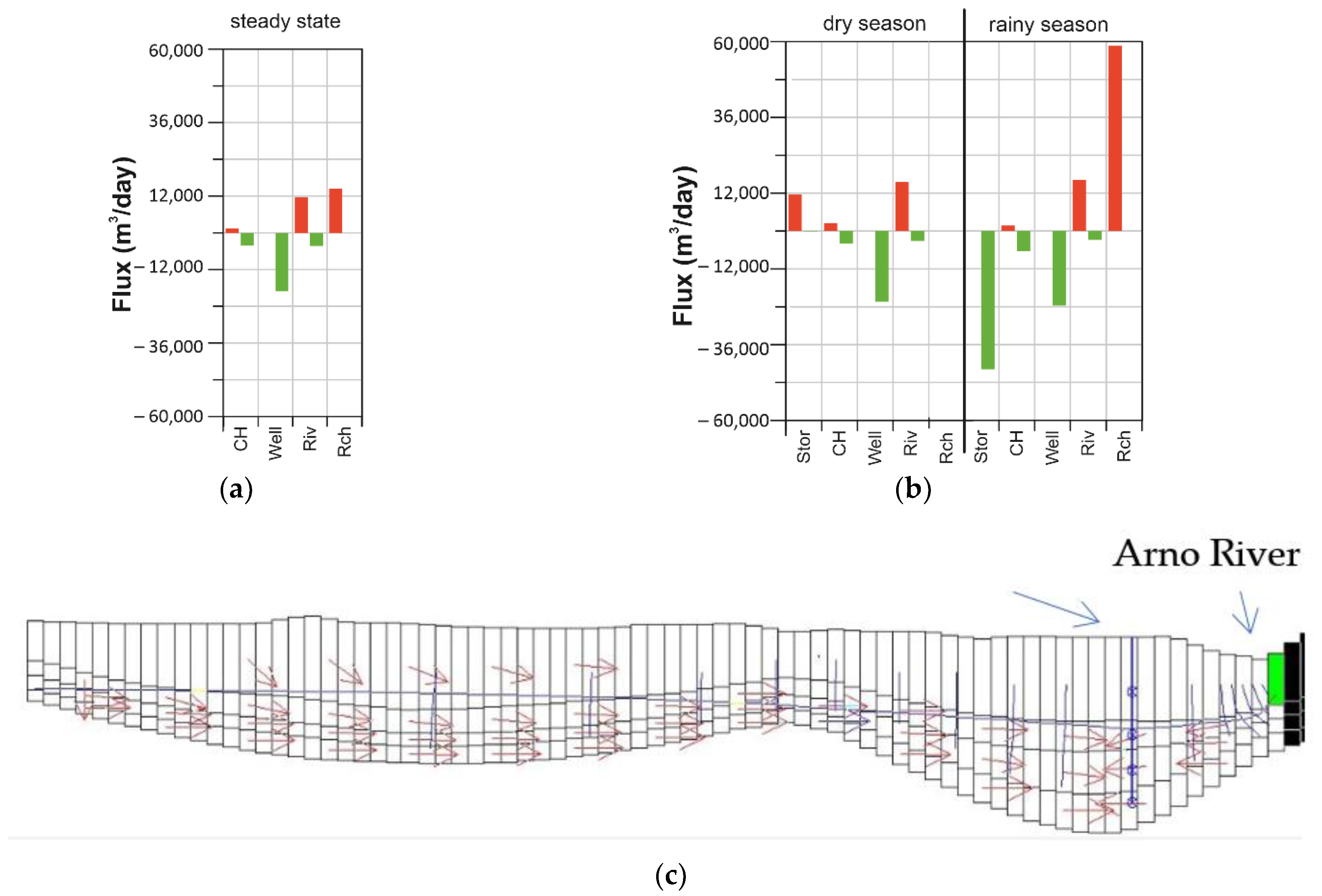
The water balance of the steady-state model (Figure 7a) indicates that the main recharge component of the aquifer is the diffuse infiltration water (Rch). The rivers seepage (Riv in red) is also significant, and this component is particularly important in the area close to the Empoli wellfield (Figure 3), as shown in the section of Figure 7c, thus confirming the indications from water isotopes and hydro-chemical tracers analyzed in previous studies [42,43]. The main outflow component from the aquifer is the wells’ withdrawal and, secondarily, with similar quantities, stream drainage (Riv in green) and natural subterranean outflow through the west sector (downstream zone).
By analyzing the water balance of the transient simulation (Figure 7b), the diffuse recharge occurring in the rainy periods is confirmed to be the most important input for the system. In the rainy seasons, almost 70% of such input contributes to water storage, which is then consumed in part during the dry season. However, in the period covered by the transient model (2016–2017 period, significantly rainy), there is a general increase in water storage with an accumulation of more than 2 million m3 of water resources. The water pumping is the main output from the aquifer (well in green).
3.1.4. Forecast Simulations
Based on the groundwater models of the Empoli aquifer system, forecast simulations were then carried out with the aim of assessing how the expected extreme climatic regimes would affect groundwater. In particular, it was assumed that a weather-climate regime similar to that of the current year and previous ones (i.e., 2003 and 2017), with several months of drought conditions, can repeat for five consecutive years.
A transient-state flow model was then created with 20 quarterly stress periods. Stress periods relating to the April–June and July–September periods were implemented with zero recharge, as occurred in 2022, whereas the stress periods in the January–March and October–December periods were implemented with low rainfall amounts similar to those of the 2003 and 2017 years. Considering that diffuse infiltration is the most important recharge component of the system, all other boundary conditions were kept constant with average values used for the steady-state model.
In Figure 8, the evolution of groundwater level at targets (wells 6A, Giardino, A and B; see Figure 5 for the location) and storage inflow in the domain during the simulation period are represented. Most observation wells (wells 6A, Giardino and B) present a more or less constant and low decrease rate that, over the entire period, results in about 1 m of drawdown. For well A, the forecasted drawdown appears more important, amounting to about 3 m in total over the period of simulation. The inflow of water storage in the groundwater flux also decreases over the entire period, reducing by about 50%, even if it presents a sub-cycle of increasing-decreasing correspondence to rainy and dry season alternations.
3.2. Data-Driven Model of the Brenta Aquifer System
A consistent, continuous monitoring network made up of several meteoric, hydrometric, and piezometric stations is available for the foothill aquifer system of the River Brenta. The availability of a very long time series allowed for the development of an MLRA of the piezometric levels of groundwater in the middle-high plain. The regression model aims to make predictions on the development of the groundwater level in expected weather and climate conditions in order to provide useful information for steering the best water management practices in a zone where strategic groundwater exploitation systems are located.
3.2.1. Conceptual Model
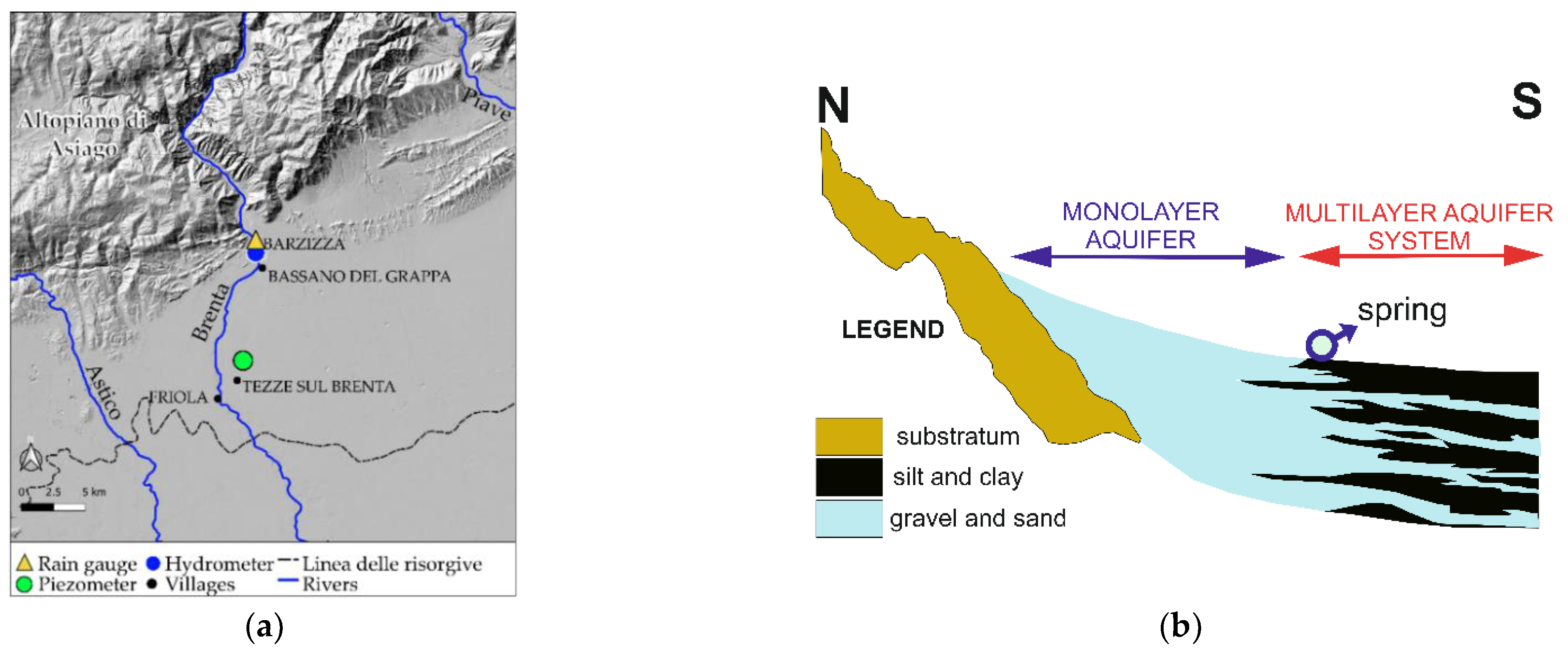
The middle-high plain of the River Brenta is located in the Veneto region between the Pre-Alps, and a series of aligned springs called the “Linea delle Risorgive” (Figure 9a). The plain is mainly made up of glacio-fluvial and fluvial sediments (Late Pleistocene-Holocene) deposited by Astico, Brenta, and Piave rivers from the west to east [47].
In particular, the high plain is essentially made up of a very thick layer of unconsolidated conglomerates (gravels and pebbles), whereas the middle plain consists of gravelly deposits intercalated by levels of sporadic cemented sands and silt and clay [49,50,51,52]. Thanks to the general high permeability of deposits and to the high amount of annual rainfall, which varies between 1200 and 1500 mm/year, an important foothill aquifer system develop in this area. The northernmost portion of the aquifer system is substantially unconfined, being hosted into the thick single-layer of gravelly pebbly alluvial deposits (Figure 9b), whereas the southern portion of the aquifer becomes semi-confined and multilayer consisting of gravelly deposits intercalated by level with low permeability [49,51,53]. The inhomogeneous hydrogeological conditions are not only moving north–south, from downward the foothill zone, but also laterally, in the east–west direction, for the presence of other foothill alluvium fan systems belonging to different rivers. The recharge of groundwater resources depends on different mechanisms, whose prevalence varies according to the sectors of the aquifer system. The focused recharge is dominant in the zone crossed by the River Brenta over the high plain, where this watercourse loses important water quantity towards the aquifer [49,51,53]. Local rainfall infiltration becomes the main recharge mechanism away from the main river path.
3.2.2. Model Implementation and Validation
The MLRA of the piezometric level has been realized using data recorded by: one pluviometry station (PS), one hydrometric station (HS) and one piezometer (Figure 9a). These points were chosen based on the conceptual model discussed above in order to represent the relationship between surface water and groundwater that significantly affect the groundwater flow in the system. the selected pluviometry station is located at Bassano del Grappa (127 m a.s.l.), whereas the used hydrometric station is located in Barziza, near Bassano del Grappa, at an altitude of 106 m a.s.l. and immediately downstream of the mountain area. The selected piezometer is located on the hydrographic left of the River Brenta in the middle-high part of the plain, near Tezze sul Brenta, in a zone where the river feeds the aquifer and a few kilometers upstream with respect to a wells field of regional importance. The monthly data from 2010 to 2022 recorded from rainfall and hydrometric stations have been collected on the ARPAV website [54]. The piezometric levels derive from continuative monitoring performed by ETRA SpA, which has provided the hourly data from 2010 to 2020. The hourly piezometric level data has been transformed into average monthly data to compare them with rainfall and hydrometric level data.
To implement the MLRA of piezometric level, the first step of the data processing was the gaps filling by linear interpolation method, which mainly concerned the rainfall series. The second step was to obtain the maximum correlation between dependent and independent variables performing the transformation of raw data. In particular, rainfall (Rf) and the hydrometric level (HL) have been identified as independent variables, whereas the piezometric level (PL) is the dependent variable. The maximum correlation coefficient between PL and Rf has been obtained by shifting of 1 lag (i.e., 1 month) and by using the moving average at 12 months of the Rf series. On the other hand, the maximum correlation coefficient between PL and HL has been obtained only by shifting 1 lag (i.e., 1 month) in the HL series. Moreover, in order to obtain a more reliable model, the multicollinearity between the independent variables was taken into account. Multicollinearity exists whenever two or more of the independent variables in a regression model are moderately or highly correlated. For this reason, the VIF (Variation Inflation Factor [55,56]) has been calculated in Equation (1):
where R2 represents the unadjusted coefficient of determination for regressing, and k, the predictor variable, on the remaining ones. In practice, VIF is calculated by performing a linear regression of predictor variables and then obtaining R2 (coefficient of determination) from that regression.
VIFk = 1/(1 − R2k)
Taking into account the correlation coefficient between Rf and HL, the VIF value is 1.8. Up to now, there is not an accepted cutoff value for VIF; nevertheless, values greater than 10 are generally considered indicators of multicollinearity problems.
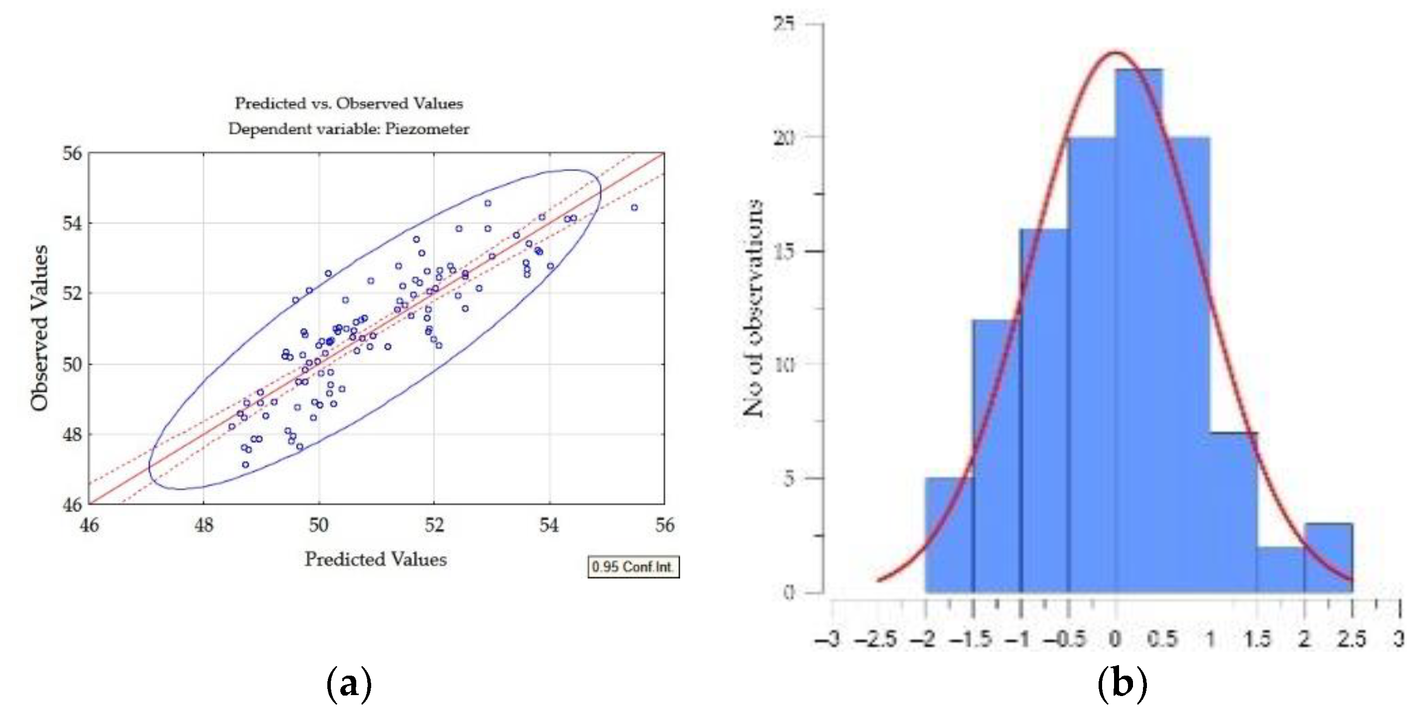
The best MLRA model has been chosen by comparing the observed vs. predicted data (Figure 10). Data from January 2010 to December 2019 of the PL, HL and Rf have been used, and the mathematical expression is represented by the following equation:
PL = HL × 3.225 + Rf × 0.031 − 295.897
Equation (2) shows that the River Brenta is more influential than the rainfall on the piezometric level variations at the selected point of monitoring.
The scatterplot in Figure 10a shows the regression line between predicted and observed values with R2 = 0.69, and the regression bands and the ellipse with 95% confidence interval [57], whereas the Figure 10b shows that residuals have a Normal distribution (Lilliefors and Shapiro–Wilk tests) at 0.05 significance level. Moreover, no data exceed the threshold of ±2.5 σ.
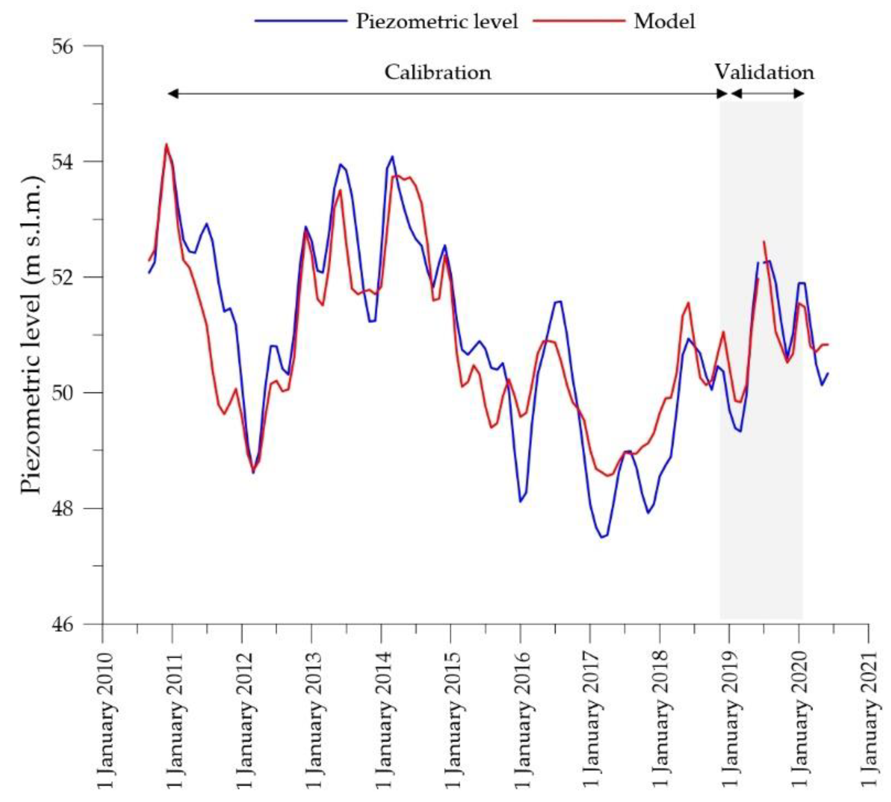
The model has been validated using rainfall and hydrometric level data from August 2019 to December 2020. Even for validation, a residual analysis has been performed, and it results in a Normal distribution (Lilliefors and Shapiro–Wilk tests) of residuals that have a 0.05 significance level and values that do not exceed the limit of ±1.5 σ.
The MLR model replicates quite well the general trend and behavior of the piezometric level (Figure 11), aside from slight existing errors for the absolute value in a few sub-periods (e.g., 2016–2018).
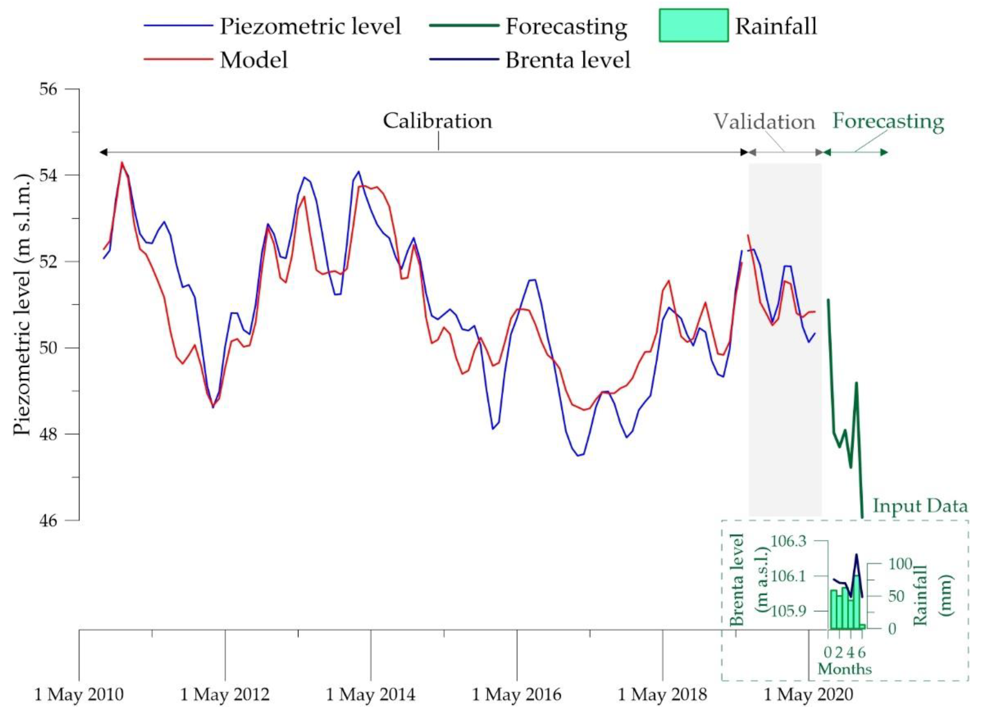
3.2.3. Forecasting Simulation
The implemented MLR results are sufficiently reliable to perform a forecasting simulation of the piezometric level 6 months ahead. The forecast has been elaborated for the prospective of simulating a particularly dry period, such as the summer of 2003 and 2022. Data on hydrometric levels and rainfall similar to the dry periods of 2003 and 2022 have been used to achieve this goal. Figure 12 displays the model with the results of forecasting simulation (green line) and used data rainfall. The simulation shows that, in the case of a particularly dry period (monthly rainfall lower than 100 mm), the piezometric level abruptly decreases, reaching very low-level values in a few months. It is important to note that when rainfall occurs, even though in medium-low quantity, the groundwater level increases very quickly. However, such as recovering is not sufficient for return in the hydrodynamic state ante-dry period.
3.3. Combined Approach of Data-Driven and Process-Based Models for the Magra Lower-Valley Aquifer System
The aquifer of the Lower Magra Valley is the main source of water for drinking, industrial and agricultural purposes in the area of La Spezia (SE Liguria, Italy). Groundwater flow is, for a significant part, controlled by streamwater infiltration, which affects both groundwater level and quality [58]. So, the groundwater system is exposed to high vulnerability, both in terms of quality and quantity, not only in relation to human activities but also towards climate conditions.
In view of its importance, as well as vulnerability, the system has been the subject of numerous quantitative and qualitative monitoring activities appropriately distributed throughout the territory and with a robust time series of historical data. This availability, and the recharge mechanisms, made it possible and necessary to perform the data-driven and process-based combined approach, thus aspiring to a process-based model that, under anticipated climate conditions, predicts all groundwater systems response but also takes into account the climate-dependent evolutions of some boundary conditions of the same model.
This study is aimed to develop this kind of predictive flow and transport model in order to achieve information on the vulnerability “sensu lato” of the Magra Valley aquifer system and to evaluate its behavior in anticipated climate scenarios.
3.3.1. Conceptual Model
The aquifer of the Magra Lower Valley extends in a flat plain, within which two main rivers (Magra and Vara) flow. These rivers are characterized by a wide variation of water level and chemical composition due to the combination of rainfall regime and the presence of thermal springs in the inner part of the catchment area, which are characterized by a sulphate-dominant chemical composition [58,59].
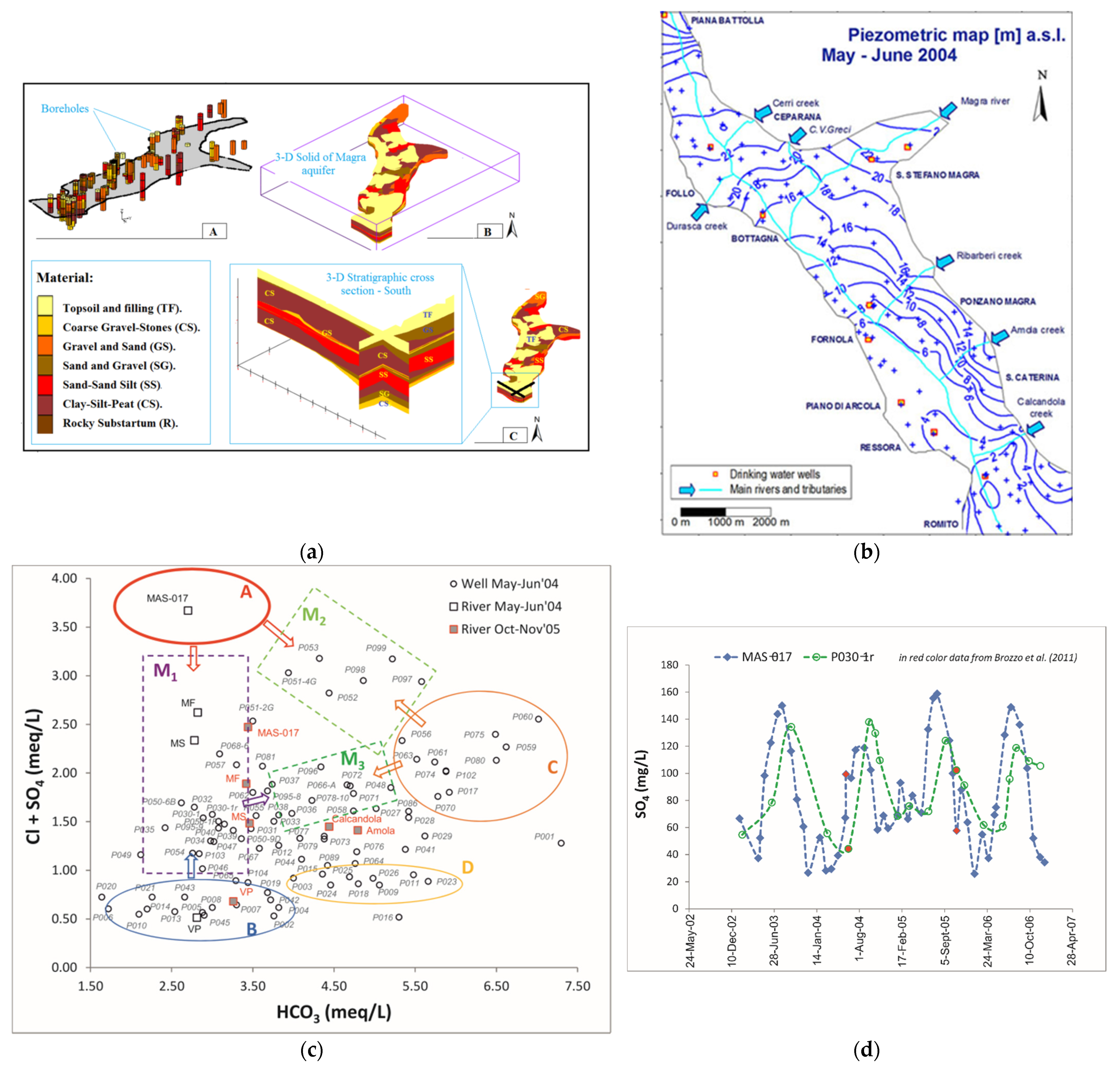
The conceptual model was achieved by elaborating and comparing geology, stratigraphy, hydrogeology, geochemistry, and isotope data (Figure 13). The aquifer is mostly unconfined and made up of gravel and sand (K ranging from 10−5 to 10−3 m/s). The groundwater flow results show it is widely controlled by stream water infiltration, which affects water levels and water quality. In particular, the wide range of variation of some particular chemical species in the stream water influences groundwater chemistry on a seasonal basis (Figure 13d). Based on data elaboration, main recharge components and their mixing processes have been identified (Figure 14) and subsequently mathematically represented in the process-based model.
3.3.2. Process-Based and Data-Driven Models Implementation and Calibration
Based on the conceptual model, flow and transport process-based models were implemented and developed using MODFLOW and MT3DMS codes and have been calibrated in both steady-state and transient conditions over the 2004–2011 period (in which the experimental data are available). For more details on the implementation of flow and transport process-based models, see the work of El Mezouary et al. [60].
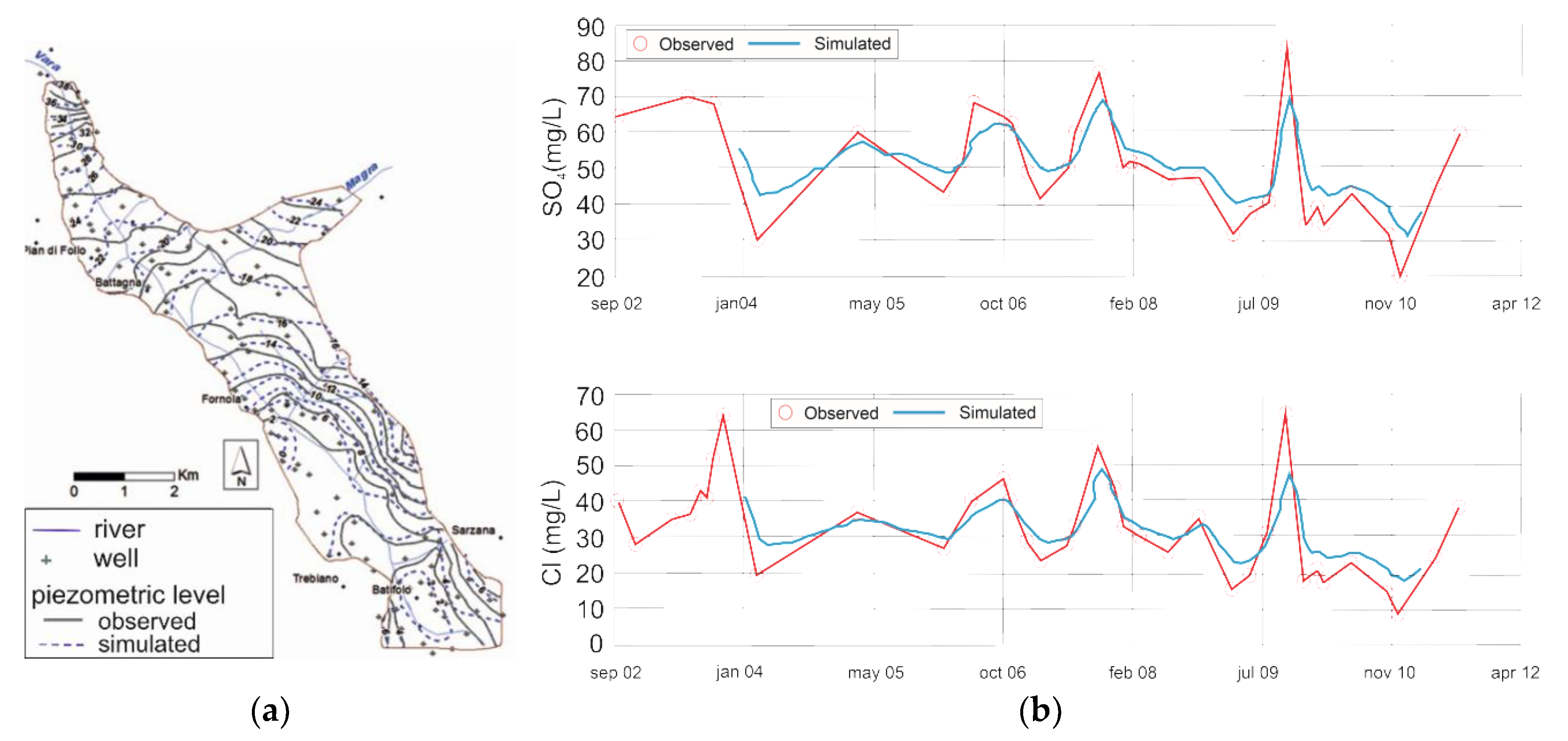
The calibration of the models showed a high congruence with the observed data for both piezometric levels and chemical concentrations (Figure 15), thus indicating very good representativeness of the models. The results of the process-based models confirmed the importance of the Magra river in the water balance of the aquifer (input of about 66%) and in the chemical composition of groundwater.
Given the strong dependence of the aquifer on river waters, both quantitatively and qualitatively, the implementation of river-related boundary conditions is, therefore, essential for carrying out forecast simulations. This justifies the need to create plausible data sets of hydrometric level and concentration of chemical species in the river water, to investigate their dependence on the expected weather and climate data and implement such analysis in the forecasting simulations performed with the process-based model.
For this purpose, fully synthetic datasets have been generated as a training set of the data-driven scheme, with input variables inspired by selected climate models and input/output relationships estimated by past observations (Figure 2).
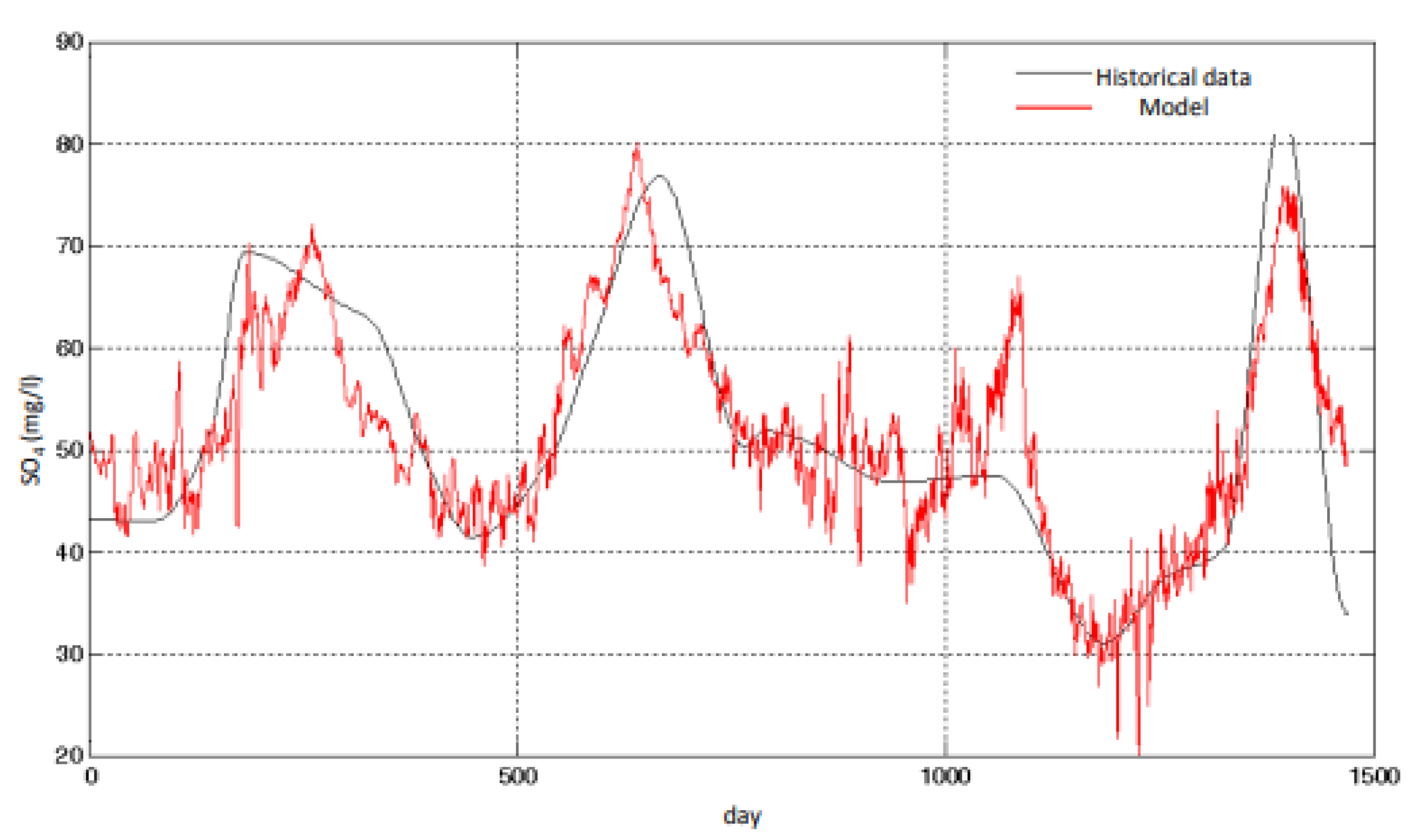
In Figure 16, a good agreement between modeled and real data (in this case, groundwater SO4 concentration in the River Magra) is shown, derived by the application of the data-driven model for the calibration period 2004–2011.
3.3.3. Forecasting Simulation
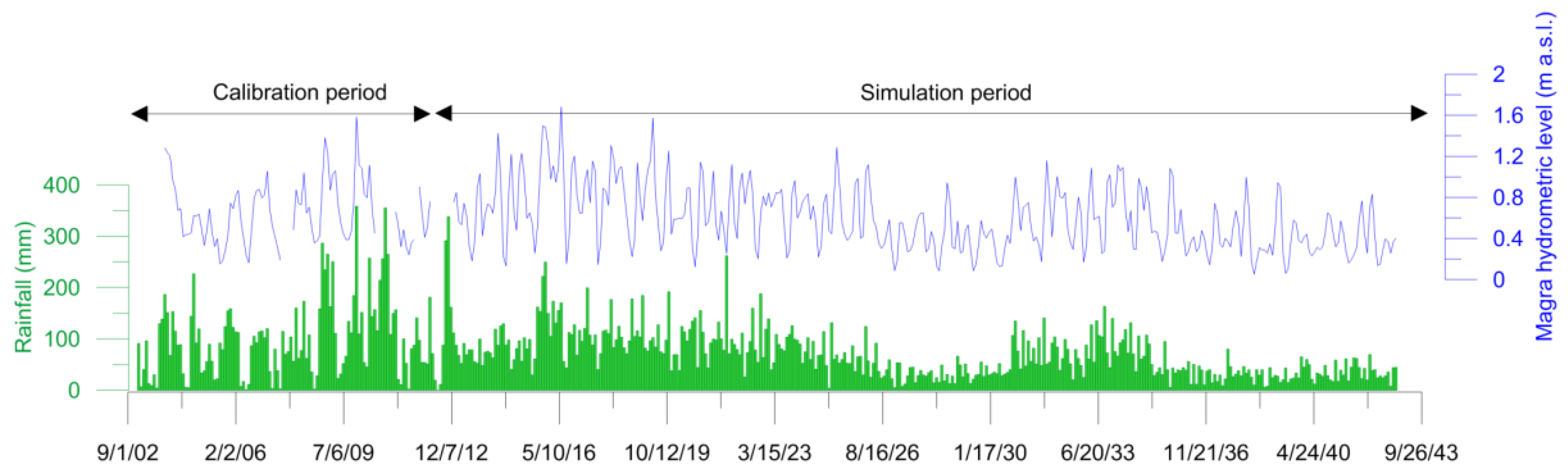
As previously stated, to develop predictive flow and transport models in order to evaluate the aquifer behavior in anticipated climate scenarios, a process-based and data-driven modeling combined approach was applied. The data-driven models were built in order to determine boundary conditions (e.g., rivers and constant head or general head boundaries) of the process-based model under hypothetic future climate scenarios (Figure 17), characterized by some dry and low-rainy periods.
Based on such hypothetic scenarios, an experimental and exemplified run of the flow-transport model for 30 years ahead was performed. In Figure 18, it is possible to observe an SO4 concentration map of the aquifer and SO4 time series of specific points. From the map, the strong chemical influence of the River Magra waters on groundwater quality is evident, especially close to Fornola wellfield, which attracts even more surface water. This influence can also be observed at the two representative points of the aquifer outside the wellfield (Figure 18), where a variation in the concentration of sulphates can be observed, mainly linked to the rainfall regime, especially at the point closest to the wellfield. It is interesting to observe how the sulphate value at the point located furthest from the wellfield remains higher and approximately constant over time following dry periods.
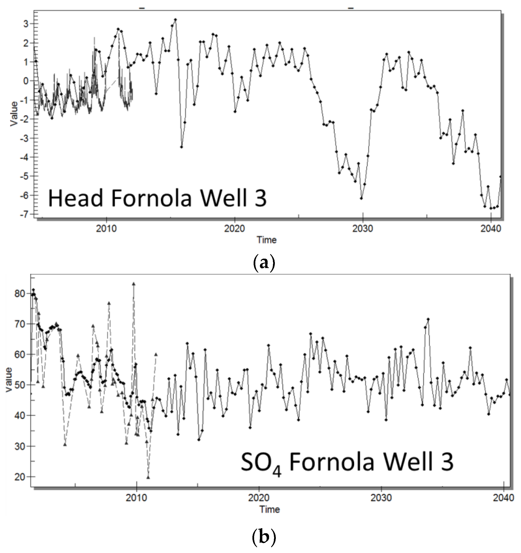
Finally, by observing the piezometric level and sulphate concentration in a well for drinking water (Fornola 3) in the wellfield (Figure 19), it is possible to observe how, after a medium-long period characterized by a low value of rainfall (e.g., 2025–2030), the aquifer system reacts with significant decreasing of piezometric level and relative increasing of SO4 solute concentration. After these periods, the sulphate concentration continues to vary greatly depending on the rainfall regime, although it generally seems to increase or at least fluctuate around a higher average value.
4. Discussion and Conclusions
The performed groundwater modeling for the three different systems first provides information about the main hydrological processes and elements regulating the groundwater flow in the systems themselves. On the other hand, the different approaches adopted accordingly to the specificities of the sites enabled the forecasting of groundwater behavior under anticipated climate conditions.
The calibrated process-based model of the Empoli aquifer system as the diffuse recharge represents the main highlighted input in this case. Rivers also contribute to groundwater flow, but this component appears secondary with respect to diffuse infiltration. Furthermore, the system denotes a good capability for water storage, which is an important part of the total water budget (Figure 7). Such as hydrodynamic features are favorable for mitigating, at least in short periods (a few years), the effects of drought events, which have become more and more frequent in the last decades and also in the Mediterranean regions [61]. The forecasting provided by the model seems to confirm these characteristics and behaviors for the Empoli aquifer system. Under drought conditions (very similar to those that occurred in recent periods) repeated for some consecutive years, the model, in general, highlighted that the decreasing groundwater level is moderate. It is very likely that the storage capability of the system that is capitalizing the small amount of effective yearly rainfall attenuates and dilutes over time the groundwater drawdown (Figure 8).
The Brenta River’s aquifer system is extensive, strategic for water supply, and characterized by inhomogeneity in terms of hydrogeology, recharge components, and water exploitation distribution as well. In these conditions, it becomes important to provide models able to describe the local groundwater behavior over time. This is the case of the data-driven model developed for a significant piezometric monitoring point sited near the losing River Brenta. The groundwater level evolution has been well-reproduced, starting from precipitation and hydrometric data as input. The equation describing the model confirms the close dependence of groundwater from the river in the analyzed zone and, therefore, the high sensitivity of the aquifer with respect to the meteo-climate regime, which directly and abruptly affects the regime of the River Brenta. In view of this high sensitivity, the forecast of groundwater level evolution under a relatively dry period of six months, similar to what occurred during the 2022 and 2003 years, was performed. Results point out a drawdown of groundwater level of more than 3 m (Figure 12) in a few months, thus remarking the very high sensitivity of the aquifer to climate extremes, as well as the need to plan actions for mitigating risks for water supply, given the regional importance of the wellfields present in this zone. Given the straight dependence of the local groundwater quantity from the hydrometric level, an advantage in making available a model that an equation estimates, such as a relationship, is the possibility of solving the same equation for a set of minimum progressive hydrometric levels with respect to when the piezometric levels do not decrease under safety threshold values. In this way, a water manager can provide actions over the catchment for maintaining the hydrometric levels over certain critical values once the territory dotes specific hydro-infrastructures able to regulate the dynamics of the watercourse.
For what concerns the aquifer of the River Magra Lower Valley, here a combined approach of modeling has been proposed in order to obtain more efficient information through the developed model. Indeed, the aquifer system is well-described by means of data from geology, hydrogeology and geochemistry, enough to develop a process-based model able to reproduce the overall behavior of the system for groundwater quantity and quality. At the same time, and as the same process-based calibrated models confirm, the groundwater flow and transport deeply depend on some boundary conditions very sensitive to the hydro-climate regime, such as the River Magra. In these situations, to provide hypothetic sets of data for such boundaries (e.g., streamwater level or streamwater chemical concentration) in case of forecasting by a process-based model can be a real risk of failure, given the probable incongruence between such input data and the input data concerning the diffuse recharge directly deducible from the anticipated climate condition. In this kind of context, it is therefore evident that the use of a data-driven model able to link the evolution of certain boundary conditions with the anticipated climate conditions represents a significant advantage in terms of the efficiency and reliability of the predictive model. The so-developed model for the River Magra aquifer demonstrates that, under relatively dry climate conditions, the river is responsible for a relative worsening of the water quality, mainly tied to an increase or a relatively high and constant value of sulphate in groundwater. The dry weather results in a sort of persistent base flow in the River Magra, which is mainly dependent on the mountain thermal springs with sulphate chemical facies. The losing character of the river and the general groundwater flow path network promote the diffusion of such sulphate components into the aquifer for an extensive sector (Figure 18).
All models developed in this work enable a better understanding of the aquifer systems’ functioning and the sensitivity of groundwater flow to climate change. Generally speaking, the applicability, limitations and accuracy of the different modeling approaches are deeply dependent on the aquifer systems’ features, functioning, and data availability as well.
The process-based model requires a large amount of information (e.g., the geometry of the main hydrogeological units) and data (e.g., hydraulic parameters value) well-distributed over the domain and time in order to achieve accurate results. At the same time, this type of approach makes it possible to model the behavior of the whole groundwater system under study.
The data-driven models require a number of observations that ideally encompass the values range of all expected stresses to the system, but it is independent of the knowledge of numerous parameters that are often difficult to find. Data-driven models are powerful, but they only estimate a given variable on one or more individual points and do not return information on a domain scale (e.g., water balance).
The integrated approach of data-driven/process-based modeling represents a novel outcome resulting in a very efficient tool for forecasting aquifer systems’ evolution when also boundary conditions significantly affecting the behavior of such systems are subjected to evolve under expected climate scenarios. As these conditions are frequent in aquifer systems, the proposed integrated modeling represents a very powerful approach, even if it needs a deep knowledge of the system as a whole and large datasets.
As a general outcome, this manuscript remarks that, for modeling groundwater resources and forecasting its evolution with respect to climate change, the choice of the suitable numerical modeling methodology is mandatory, and it mainly depends on the specific aquifer features that result in different ways to be sensitive to climate. Only through this approach is it possible to provide efficient groundwater forecasts that are able to steer water management plans and actions aimed at mitigating the effects of climate change.
Author Contributions
Conceptualization, M.M. and M.D.; Methodology, M.M., B.R. and A.S.; Validation, M.M., L.F. and A.S.; Data curation, M.M., L.F., A.S. and M.D.; Writing—original draft preparation, M.M., M.D. and L.F.; Writing—review and editing, M.M., M.D. and L.F.; Visualization, M.M. and G.M.; Supervision, M.D. and M.M.; Project coordination, M.D. and M.M. All authors have read and agreed to the published version of the manuscript.
Funding
This research was co-funded in part by Tuscany Water Authorities, Brenta Basin Council and the Italian national project ACQUASENSE (Industria2015- Project number: MI01_00223).
Data Availability Statement
Data are available upon request to the corresponding author.
Acknowledgments
The authors would like to thank the Tuscan Water Authority (AIT) and the Brenta Basin Council for co-funding this study and Ingegnerie Toscane and ETRA water service for sharing their data. The authors would also like to thank the five referees and the editors who contributed to improving the manuscript with their advice.
Conflicts of Interest
The authors declare no conflict of interest.
References
- United Nations. The United Nations World Water Development Report 2022: Groundwater: Making the Invisible Visible; UNESCO: Paris, France, 2022; p. 225. ISBN 978-92-3-100507-7. [Google Scholar]
- Hiscock, K.M. Groundwater in the 21st century—meeting the challenges. In Sustaining Groundwater Resources: A Critical Element in the Global Water Crisis, in International Year of Planet Earth; Anthony, J., Jones, A., Eds.; Springer: Dordrecht, Netherlands, 2011; pp. 207–225. [Google Scholar] [CrossRef]
- Zhu, Y.; Balke, K.D. Groundwater protection: What can we learn from Germany? J. Zhejiang Univ. Sci. 2008, 9, 227–231. [Google Scholar] [CrossRef] [PubMed] [Green Version]
- Baoxiang, Z.; Fanhai, M. Delineation methods and application of groundwater source protection zone. In Proceedings of the Water Resource and Environmental Protection (ISWREP), 2011 International Symposium, (IEEE Conference Publications), Xi’an, China, 20–22 May 2011; Volume 1, pp. 66–69. [Google Scholar] [CrossRef]
- Martınez Navarrete, C.; Grima Olmedo, J.; Duran Valsero, J.J.; Gomez, J.D.; Luque Espinar, J.A.; de la Orden, G.J.A. Groundwater protection in Mediterranean countries after the European water framework directive. Environ. Geol. 2008, 54, 537–549. [Google Scholar] [CrossRef]
- WBCSD Facts and Trends–Water. World Business Council for Sustainable Development. Available online: https://www.wbcsd.org/Programs/Food-and-Nature/Water/Resources/Water-Facts-and-trends (accessed on 1 September 2022).
- Siebert, S.; Burke, J.; Faures, J.M.; Frenken, K.; Hoogeveen, J.; Döll, P.; Portmann, F.T. Groundwater use for irrigation—A global inventory. Hydrol. Earth Syst. Sci. 2010, 14, 1863–1880. [Google Scholar] [CrossRef] [Green Version]
- Wada, Y.; Van Beek, L.P.H.; Van Kempen, C.M.; Reckman, J.W.T.M.; Vasak, S.; Bierkens, M.F.P. Global depletion of groundwater resources. Geophys. Res. Lett. 2010, 37, L20402. [Google Scholar] [CrossRef] [Green Version]
- Rosegrant, M.W.; Cai, X.; Cline, S.A. World Water and Food to 2025: Dealing with Scarcity; International Food Policy Research Institute: Washington, DC, USA, 2002; p. 322. [Google Scholar]
- Milly, P.C.D.; Dunne, K.A.; Vecchia, A.V. Global pattern of trends in streamflow and water availability in a changing climate. Nature 2005, 438, 347–350. [Google Scholar] [CrossRef]
- Hirabayashi, Y.; Mahendran, R.; Koirala, S.; Konoshima, L.; Yamazaki, D.; Watanabe, S.; Kim, H.; Kanae, S. Global flood risk under climate change. Nat. Clim. Chang. 2013, 3, 816–821. [Google Scholar] [CrossRef]
- Chan, D.; Wu, Q. Significant anthropogenic-induced changes of climate classes since 1950. Sci. Rep. 2015, 5, 13487. [Google Scholar] [CrossRef] [Green Version]
- Turco, M.; Palazzi, E.; von Hardenberg, J.; Provenzale, A. Observed climate change hotspots. Geophys. Res. Lett. 2015, 42, 3521–3528. [Google Scholar] [CrossRef]
- Tollefson, J. IPCC climate report: Earth is warmer than it’s been in 125,000 years. Nature 2021, 596, 171–172. [Google Scholar] [CrossRef]
- Taylor, R.G.; Scanlon, B.; Döll, P.; Rodell, M.; Van Beek, R.; Wada, Y.; Longuevergne, L.; Leblanc, M.; Famiglietti, J.S.; Edmunds, M.; et al. Ground water and climate change. Nat. Clim. Chang. 2013, 3, 322–329. [Google Scholar] [CrossRef] [Green Version]
- Ohba, M.; Arai, R.; Sato, T.; Imamura, M.; Toyoda, Y. Projected future changes in water availability and dry spells in Japan: Dynamic and thermodynamic climate impacts. Weather. Clim. Extremes 2022, 38, 100523. [Google Scholar] [CrossRef]
- Fan, Y. Groundwater. How much and how old? News Views. Nat. Geosci. 2015, 9, 93–94. [Google Scholar] [CrossRef]
- Doveri, M.; Menichini, M.; Scozzari, A. Protection of groundwater resources: Worldwide regulations, scientific approaches and case study. In The Handbook of Environmental Chemistry: Threats to the Quality of Groundwater Resources: Prevention and Control; Scozzari, A., Dotsika, E., Eds.; Springer-Verlag: Berlin/Heidelberg, Germany, 2016; Volume 40, pp. 13–30. [Google Scholar]
- Anderson, M.P.; Woessner, W.W.; Hunt, R.J. Applied Groundwater Modeling: Simulation of Flow and Advective Transport; Academic Press: Amsterdam, The Netherlands, 2015; p. 564. [Google Scholar]
- Krešic´, N.; Mikszewski, A. Hydrogeological Conceptual Site Model: Data Analysis and Visualization; CRC Press: Boca Raton, FL, USA, 2013. [Google Scholar]
- Reilly, T.E.; Harbaugh, A.W. Guidelines for Evaluating Ground-Water Flow Models; U.S. Geological Survey Scientific Investigations Report: Reston, VA, USA, 2004; Volume 5038, p. 30. [Google Scholar]
- Grodzka-Łukaszewska, M.; Nawalany, M.; Zijl, W. A Velocity-Oriented Approach for Modflow. Transp. Porous Media 2017, 119, 373–390. [Google Scholar] [CrossRef] [Green Version]
- Ginn, T.R.; Cushman, J.H. Inverse methods for subsurface flow: A critical review of stochastic techniques. Stoch. Hydrol. Hydraul. 1990, 4, 1–26. [Google Scholar] [CrossRef]
- Shapiro, A.M.; Day-Lewis, F.D. Reframing groundwater hydrology as a data-driven science. Groundwater 2022, 60, 455–456. [Google Scholar] [CrossRef]
- Curtis, Z.K.; Li, S.-G.; Liao, H.-S.; Lusch, D. Data-Driven Approach for Analyzing Hydrogeology and Groundwater Quality Across Multiple Scales. Groundwater 2017, 56, 377–398. [Google Scholar] [CrossRef] [PubMed]
- Xu, T.; Valocchi, A.J. Data-driven methods to improve baseflow prediction of a regional groundwater model. Comput. Geosci. 2015, 85, 124–136. [Google Scholar] [CrossRef] [Green Version]
- Bakker, M.; Maas, K.; Schaars, F.; von Asmuth, J.R. Analytic modeling of groundwater dynamics with an approximate impulse response function for areal recharge. Adv. Water Resour. 2007, 30, 493–504. [Google Scholar] [CrossRef]
- Sun, J.; Hu, L.; Li, D.; Sun, K.; Yang, Z. Data-driven models for accurate groundwater level prediction and their practical significance in groundwater management. J. Hydrol. 2022, 608, 127630. [Google Scholar] [CrossRef]
- Gusyev, M.; Haitjema, H.; Carlson, C.; Gonzalez, M. Use of Nested Flow Models and Interpolation Techniques for Science-Based Management of the Sheyenne National Grassland, North Dakota, USA. Groundwater 2012, 51, 414–420. [Google Scholar] [CrossRef]
- Demissie, Y.K.; Valocchi, A.; Minsker, B.; Bailey, B.A. Integrating a calibrated groundwater flow model with error-correcting data-driven models to improve predictions. J. Hydrol. 2009, 364, 257–271. [Google Scholar] [CrossRef]
- Szidarovszky, F.; Coppola, E.A.; Long, J.; Hall, A.D.; Poulton, M.M. A Hybrid Artificial Neural Network-Numerical Model for Ground Water Problems. Groundwater 2007, 45, 590–600. [Google Scholar] [CrossRef] [PubMed]
- Meixner, T.; Manning, A.H.; Stonestrom, D.A.; Allen, D.M.; Ajami, H.; Blasch, K.W.; Brookfield, A.E.; Castro, C.L.; Clark, J.F.; Gochis, D.J.; et al. Implications of projected climate change for groundwater recharge in the western United States. J. Hydrol. 2016, 534, 124–138. [Google Scholar] [CrossRef] [Green Version]
- Menichini, M.; Doveri, M. Modelling tools for quantitative evaluations on the Versilia coastal aquifer system (Tuscany, Italy) in terms of groundwater components and possible effects of climate extreme events. Acque Sotter. Ital. J. Groundw. 2020, 9, 475. [Google Scholar] [CrossRef]
- Hunt, R.J. Ground Water Modeling Applications Using the Analytic Element Method. Groundwater 2006, 44, 5–15. [Google Scholar] [CrossRef]
- Harbaugh, A.W. MODFLOW-2005, the US Geological Survey Modular Ground-Water Model: The Ground-Water Flow Process Reston, VA, USA, 6-A16, 2005: US Department of the Interior, US Geological Survey. Available online: http://pubs.er.usgs.gov/publication/tm6A16 (accessed on 1 May 2022).
- Rumbaugh, J.O.; Rumbaugh, D.B. Groundwater Vistas; Environmental Simulations Inc.: Leesport, PA, USA, 2011; p. 213. [Google Scholar]
- Jones, N.L. GMS Reference Manual. In Aquaveo; Brigham Young University: Provo, UT, USA, 2014; p. 662. [Google Scholar]
- Gallagher, M.; Doherty, J. Parameter estimation and uncertainty analysis for a watershed model. Environ. Model. Softw. 2007, 22, 1000–1020. [Google Scholar] [CrossRef]
- Chen, J.; Brissette, F.P.; Leconte, R. A daily stochastic weather generator for preserving low-frequency of climate variability. J. Hydrol. 2010, 388, 480–490. [Google Scholar] [CrossRef]
- Jones, P.G.; Thornton, P.K.; Heinke, J. Generating Characteristic Daily Weather Data Using Downscaled Climate Model Data from the IPCC’s Fourth Assessment; Project Report. 2009, p. 19. Available online: http://dspacetest.cgiar.org/handle/10568/2482 (accessed on 1 May 2022).
- Menichini, M.; Da Prato, S.; Doveri, M.; Ellero, A.; Lelli, M.; Masetti, G.; Nisi, B.; Raco, B. An integrated methodology to define Protection Zones for groundwaterbased drinking water sources: An example from the Tuscany Region, Italy. Acque Sotter. Ital. J. Groundw. 2015, 4, 21–27. [Google Scholar] [CrossRef]
- Menichini, M.; Doveri, M.; Ellero, A.; Raco, B.; Masetti, G.; Da Prato, S.; Lelli, M.; Nisi, B. Delimitazione delle Zone di Protezione Risorse Idriche destinate al consumo umano. Campo pozzi “Empoli” (FI-ATO2). In Delimitation of Water Resources Protection Zones for Human Consumption. Empoli” well field (FI-ATO2); IGG-CNR Confidential Internal Technical Report n 10988; IGG-CNR: Pisa, Italy, 2013. [Google Scholar]
- Da Prato, S.; Doveri, M.; Ellero, A.; Lelli, M.; Masetti, G.; Menichini, M.; Nisi, B.; Raco, B. Integrazioni alla Caratterizzazione geologica, idrogeologica e idrogeochimica dei Corpi Idrici Sotterranei Significativi della Regione Toscana (CISS). 11AR025 Corpo idrico del Valdarno Inferiore e Piana Costiera Pisana-zona Empoli. In Integrations to the Geological, Hydrogeological and Hydrogeochemical Characterisation of the Significant Underground Water Bodies of the Region of Tuscany (CISS) Valdarno Inferiore and Piana Costiera Pisana Water Body-Empoli Area; Technical Report IGG n° 10976; IGG-CNR: Pisa, Italy, 2012; p. 18. [Google Scholar]
- SIR-Regional Hydrological and Geological Sector. Available online: www.sir.toscana.it (accessed on 1 March 2018).
- Doveri, M.; Da Prato, S.; Masetti, G.; Menichini, M.; Raco, B.; Vivaldo, G.; Scozzari, A. Relazione Sulle Attività Svolte Nell’ambito Dell’Accordo di Collaborazione Scientifica AIT-LaMMA-IGG/CNR del 13 March 2017 IGG-CNR Confidential Internal Technical Report n° 12306; IGG-CNR: Pisa, Italy, 2020; p. 35. [Google Scholar]
- SIR-Regional Hydrological and Geological Sector. Available online: www.idropisa.it/consumi_idrici (accessed on 1 March 2018).
- Cisotto, A.; Rusconi, A.; Baruffi, F. Regional Studies of the North Adriatic Basin Authority on the Aquifers of the Veneto-Friuli Plain. Mem. Descr. Carta Geol. d’It. 2007, 76, 117–124. [Google Scholar]
- Carraro, A.; Fabbri, P.; Giaretta, A.; Peruzzo, L.; Tateo, F.; Tellini, F. Arsenic anomalies in shallow Venetian Plain (Northeast Italy) groundwater. Environ. Earth Sci. 2013, 70, 3067–3084. [Google Scholar] [CrossRef]
- Dal Prà, A.; Veronese, F. Gli acquiferi dell’alta pianura alluvionale del Brenta e i loro rapporti col corso d’acqua. Atti Istituto Veneto Sc. Lett. Arti. 1972, 5, 189–222. [Google Scholar]
- Pilli, A.; Sapigni, M.; Zuppi, G. Karstic and alluvial aquifers: A conceptual model for the plain – Prealps system (northeastern Italy). J. Hydrol. 2012, 464–465, 94–106. [Google Scholar] [CrossRef]
- Sottani, A.; Vielmo, A. Groundwater conservation and monitoring activities in the middle Brenta River plain (Veneto Region, Northern Italy): Preliminary results about aquifer recharge. Acque Sotter. Ital. J. Groundw. 2014, 3, 3. [Google Scholar] [CrossRef]
- Mayer, A.; Sültenfuß, J.; Travi, Y.; Rebeix, R.; Purtschert, R.; Claude, C.; Salle, C.L.G.L.; Miche, H.; Conchetto, E. A multi-tracer study of groundwater origin and transit-time in the aquifers of the Venice region (Italy). Appl. Geochem. 2014, 50, 177–198. [Google Scholar] [CrossRef]
- Bullo, P.; Dal Prà, A. Lo sfruttamento ad uso acquedottistico delle acque sotterranee dell’alta pianura alluvionale veneta. Geol. Romana 1994, 30, 371–380. [Google Scholar]
- ARPAV–Regional Agrncy for Environmental Prevention and Protection of Veneto. Available online: www.arpa,veneto.it (accessed on 1 January 2020).
- Freund, R.J.; Wilson, W.J. Regression Analysis: Statistical Modeling of a Response Variable; Academic Press: New York, NY, USA, 1998. [Google Scholar]
- Adnan, N.; Ahmad, M. A comparative study on some method for handling multicollinearity problems. Matematika 2006, 22, 109–119. [Google Scholar] [CrossRef]
- Tracy, N.D.; Young, J.C.; Mason, R.L. Multivariate Control Charts for Individual Observations. J. Qual. Technol. 1992, 24, 88–95. [Google Scholar] [CrossRef]
- Brozzo, G.; Accornero, M.; Marini, L. The alluvial aquifer of the Lower Magra Basin (La Spezia, Italy): Conceptual hydrogeochemical–hydrogeological model, behavior of solutes, and groundwater dynamics. Carbonates Evaporites 2011, 26, 235–254. [Google Scholar] [CrossRef]
- Menichini, M.; Doveri, M.; El Mansoury, B.; El Mezouary, L.; Lelli, M.; Raco, B.; Scozzari, A.; Soldovieri, F. Groundwater vulnerability to climate variability: Modelling experience and field observations in the lower Magra Valley (Liguria, Italy). In EGU General Assembly Conference Abstracts; EGU: Vienna, Austria, 2016. [Google Scholar]
- El Mezouary, L.; El Mansouri, B.; Kabbaj, S.; Scozzari, A.; Doveri, M.; Menichini, M.; Kili, M. Modélisation numérique de la variation saisonnière de la qualité des eaux souterraines de l’aquifère de Magra, Italie. Houille Blanche 2015, 101, 25–31. [Google Scholar] [CrossRef]
- Mathbout, S.; Lopez-Bustins, J.; Royé, D.; Martin-Vide, J. Mediterranean-Scale Drought: Regional Datasets for Exceptional Meteorological Drought Events during 1975–2019. Atmosphere 2021, 12, 941. [Google Scholar] [CrossRef]
Figure 1.
Location of the three case studies.

Figure 2.
Block diagram describing the approach for developing a flow and transport model dedicated to specific parameters based on machine learning.
Figure 2.
Block diagram describing the approach for developing a flow and transport model dedicated to specific parameters based on machine learning.

Figure 3.
Geometrical reconstruction of the horizons constituting the Empoli aquifer system.

Figure 4.
Spatial discretization in raw and column (cells of 50 × 50 m) and in 4 layers, and hydraulic properties (K in m/day) assigned.
Figure 4.
Spatial discretization in raw and column (cells of 50 × 50 m) and in 4 layers, and hydraulic properties (K in m/day) assigned.

Figure 5.
Boundary conditions and calibration target.

Figure 6.
Calibration and validation of the model: (a) graph of observed vs. simulated level (in m a.s.l.) and (b) calibration statistics of the steady-state model; (c) piezometric level (in m a.s.l.) over time (day) measured (in red) and simulated (in blue) in the Isola target continuous monitoring point and (d) piezometric level (in m a.s.l.) over time (day) measured (in red) and simulated (in blue) in the 6A target point of the Empoli profile (only one experimental datum is available for the 6A piezometer over the validation period).

Figure 7.
Water balance for (a) steady-state and (b) transient-state models in the dry and rainy seasons, and (c) section with flow line of the Empoli aquifer (for the section trace see Figure 5; CH: constant head, Riv: river, Rch: recharge).
Figure 7.
Water balance for (a) steady-state and (b) transient-state models in the dry and rainy seasons, and (c) section with flow line of the Empoli aquifer (for the section trace see Figure 5; CH: constant head, Riv: river, Rch: recharge).

Figure 8.
Simulated evolutions of storage inflow into the domain and piezometric level at observation wells A, B, and Giardino, 6A (wells location is in Figure 5).
Figure 8.
Simulated evolutions of storage inflow into the domain and piezometric level at observation wells A, B, and Giardino, 6A (wells location is in Figure 5).

Figure 9.
(a) Middle-high plain of the Brenta River and (b) schematic section of the aquifer system (modified after [48]).
Figure 9.
(a) Middle-high plain of the Brenta River and (b) schematic section of the aquifer system (modified after [48]).

Figure 10.
(a) Error values between the predicted and observed data along the regression line and (b) distribution of residuals.
Figure 10.
(a) Error values between the predicted and observed data along the regression line and (b) distribution of residuals.

Figure 11.
Calibration and validation of the piezometric level model.

Figure 12.
Forecasting simulation of 6 months using fictitious rainfall and hydrometric level data.

Figure 13.
Multidisciplinary data elaboration to develop the conceptual model [58,59]: (a) 3D reconstruction by mean borehole information (where A is available boreholes used, B is 3-D solid of Magra Aquifer and C is an example of 3-D stratigraphic cross section); (b) Piezometric map (m) a.s.l. for the “2004 May–June” period; (c) Cl + SO4 vs. HCO3 diagram (A–D letters indicate the main recharge components of the groundwater system in Figure 14 and M1–3 indicate mixing processes); (d) SO4 concentrations in the Magra River (station MAS-017) and in a drinking water well (P030-1r) located very close to the river.

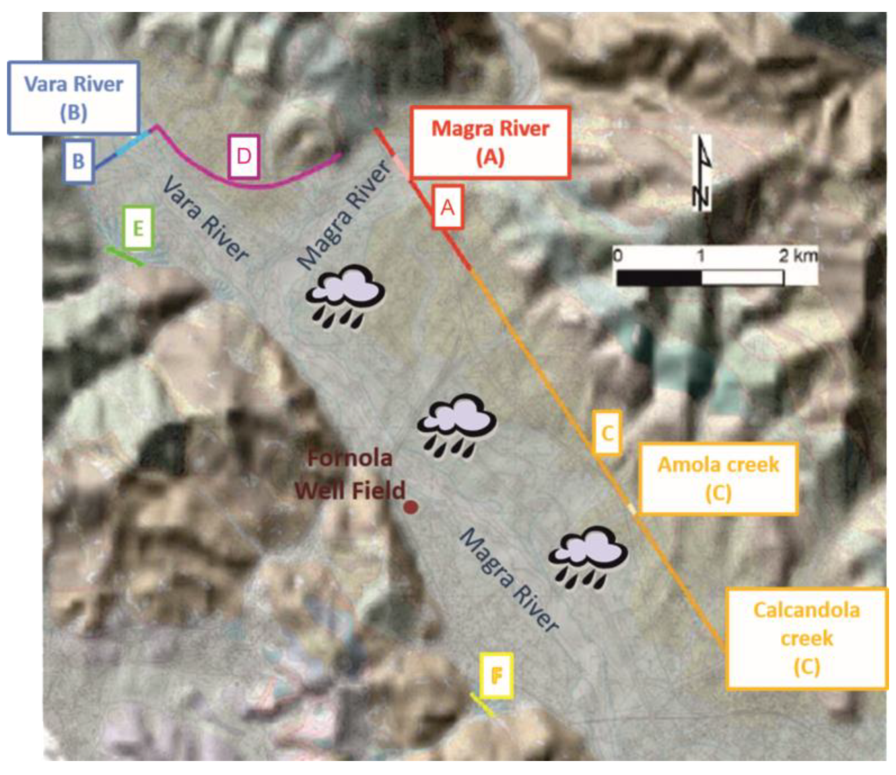
Figure 14.
Simplified sketch map showing the main recharge components of the groundwater system [53]: A—feeding from River Magra and its alluvial fan; B—feeding from River Vara and its alluvial fan; C—groundwater transfer from western hills and secondary input from minor creeks; D—groundwater transfer from northern hills; E and F—groundwater recharge from secondary creeks flowing in the western sectors.

Figure 15.
Calibration of flow and transport model: (a) Observed and simulated piezometric head [60] (b) SO4 and Cl observed and simulated value at their respective time (2004–2011) [60].

Figure 16.
Observed SO4 concentration (in grey) and calculated (in red) by the model for observation points of the Magra River.
Figure 16.
Observed SO4 concentration (in grey) and calculated (in red) by the model for observation points of the Magra River.

Figure 17.
Rainfall and Magra hydrometric level for the calibration period (2004–2011) and forecasting simulation period (2012–2042).
Figure 17.
Rainfall and Magra hydrometric level for the calibration period (2004–2011) and forecasting simulation period (2012–2042).

Figure 18.
Map and time series of SO4 concentration in the calibration and prediction periods.

Figure 19.
Time series of piezometric value (a) and SO4 concentration (b) for Fornola Well 3 in the calibration and prediction periods.
Figure 19.
Time series of piezometric value (a) and SO4 concentration (b) for Fornola Well 3 in the calibration and prediction periods.


Table 1.
Annual water consumption of each type of well.
| Water Consumption (Mm3) | Use |
|---|---|
| 8 | Drinkable |
| 0.2 | Domestic |
| 2.2 | Industrial |
| 0.5 | Agricultural |
Publisher’s Note: MDPI stays neutral with regard to jurisdictional claims in published maps and institutional affiliations. |
© 2022 by the authors. Licensee MDPI, Basel, Switzerland. This article is an open access article distributed under the terms and conditions of the Creative Commons Attribution (CC BY) license (https://creativecommons.org/licenses/by/4.0/).
Share and Cite
MDPI and ACS Style
Menichini, M.; Franceschi, L.; Raco, B.; Masetti, G.; Scozzari, A.; Doveri, M. Groundwater Modeling with Process-Based and Data-Driven Approaches in the Context of Climate Change. Water 2022, 14, 3956. https://doi.org/10.3390/w14233956
AMA Style
Menichini M, Franceschi L, Raco B, Masetti G, Scozzari A, Doveri M. Groundwater Modeling with Process-Based and Data-Driven Approaches in the Context of Climate Change. Water. 2022; 14(23):3956. https://doi.org/10.3390/w14233956
Chicago/Turabian StyleMenichini, Matia, Linda Franceschi, Brunella Raco, Giulio Masetti, Andrea Scozzari, and Marco Doveri. 2022. "Groundwater Modeling with Process-Based and Data-Driven Approaches in the Context of Climate Change" Water 14, no. 23: 3956. https://doi.org/10.3390/w14233956
Note that from the first issue of 2016, this journal uses article numbers instead of page numbers. See further details here.