
Assessment of Implementing Land Use/Land Cover LULC 2020-ESRI Global Maps in 2D Flood Modeling Application

1
Hydrology and Drainage Department Manager, Euroconsult, Cairo 11736, Egypt
2
Irrigation and Hydraulics Engineering Department, Faculty of Engineering, Cairo University, Giza 12613, Egypt
*
Author to whom correspondence should be addressed.
Water 2022, 14(23), 3963; https://doi.org/10.3390/w14233963
Submission received: 23 October 2022
/
Revised: 19 November 2022
/
Accepted: 30 November 2022
/
Published: 5 December 2022
(This article belongs to the Special Issue The Impact of Climate Change and Land Use on Water Resources)
Abstract
:Floods are one of the most dangerous water-related risks. Numerous sources of uncertainty affect flood modeling. High-resolution land-cover maps along with appropriate Manning’s roughness values are the most significant parameters for building an accurate 2D flood model. Two land-cover datasets are available: the National Land Cover Database (NLCD 2019) and the Land Use/Land Cover for Environmental Systems Research Institute (LULC 2020-ESRI). The NLCD 2019 dataset has national coverage but includes references to Manning’s roughness values for each class obtained from earlier studies, in contrast to the LULC 2020-ESRI dataset, which has global coverage but without an identified reference to Manning’s roughness values yet. The main objectives of this study are to assess the accuracy of using the LULC 2020-ESRI dataset compared with the NLCD 2019 dataset and propose a standard reference to Manning’s roughness values for the classes in the LULC 2020-ESRI dataset. To achieve the research objectives, a confusion matrix using 548,117 test points in the conterminous United States was prepared to assess the accuracy by quantifying the cross-correspondence between the two datasets. Then statistical analyses were applied to the global maps to detect the appropriate Manning’s roughness values associated with the LULC 2020-ESRI map. Compared to the NLCD 2019 dataset, the proposed Manning’s roughness values for the LULC 2020-ESRI dataset were calibrated and validated using 2D flood modeling software (HEC-RAS V6.2) on nine randomly chosen catchments in the conterminous United States. This research’s main results show that the LULC 2020-ESRI dataset achieves an overall accuracy of 72% compared to the NLCD 2019 dataset. The findings demonstrate that, when determining the appropriate Manning’s roughness values for the LULC 2020-ESRI dataset, the weighted average technique performs better than the average method. The calibration and validation results of the proposed Manning’s roughness values show that the overall Root Mean Square Error (RMSE) in depth was 2.7 cm, and the Mean Absolute Error (MAE) in depth was 5.32 cm. The accuracy of the computed peak flow value using LULC 2020-ESRI was with an average error of 5.22% (2.0% min. to 8.8% max.) compared to the computed peak flow values using the NLCD 2019 dataset. Finally, a reference to Manning’s roughness values for the LULC 2020-ESRI dataset was developed to help use the globally available land-use/land-cover dataset to build 2D flood models with an acceptable accuracy worldwide.
1. Introduction
Over the past few decades, natural disasters have seriously damaged both natural and man-made settings. One of the riskiest situations involving water is flooding, which is primarily responsible for fatalities, damage to infrastructure, and financial losses. Because flood events are occurring more frequently, with larger sizes, and more intensely, there is currently a growing global awareness of the need to mitigate flood damage [1]. The Diffusion Wave Equation (DWE) is an approximated shape of the shallow water equations (SWE) which is often used to model overland flows such as floods, dam breaks, and flows through vegetated areas. Diffusive shallow water (DSW) further simplifies the SWE by assuming that the horizontal momentum can be linked to the water height through an empirical formula, such as Manning’s [2]. The hydraulic simulation models are crucial instruments for comprehending the hydraulic properties of river-system flow [2].
The roughness coefficient (or Manning’s coefficient) is a significant hydraulic parameter, particularly in hydraulic modeling [3,4]. Specific values for the empirical parameters, such as Manning’s coefficient n, are frequently ambiguous due to the complexity of hydraulic engineering. The channel surface roughness, bed material, vegetation, channel alignment and irregularities, channel form and size, stage and discharge, suspended sediment load and bed sediment loads, etc., are all included in the roughness coefficient (Manning’s n) as an empirical parameter [5]. Several past empirical formulas have been proposed for estimating the surface roughness (n) values in practical problems [6].
Several researchers proposed several approaches for determining Manning’s roughness values n [7,8,9]. Parhi calibrated and validated the value of the roughness coefficient (n) for the Mahanadi River in Odisha using the HEC-RAS model (India). In the calibration and verification, Parhi considered the floods of 2001 and 2003 [10]. Additionally, Shamkhi and Attab investigated and calculated the value of n downstream of the Kut Barrage in Wasit, Iraq, using the HEC-RAS model [11]. Using inversion techniques, Calo et al. calculated the distributed Manning’s coefficient directly from water height measurements. To do this, an inverse problem was created for calculating n using measurements of the water height obtained from sensors and infrared imaging [2]. Using HEC-RAS software, Abbas et al. investigated the idea of a hydraulic model to calculate Manning’s coefficient n of the Tigris River along 3.5 km in the Maysan Governorate, southern Iraq [3]. In flood inundation modeling and mapping, Papaioannou et al. examined the uncertainty caused by the roughness values on hydraulic models. The initial values of Manning’s n roughness coefficient are derived from field surveys and empirical formulas. To represent the estimated roughness values, a variety of theoretical probability distributions are fitted and evaluated for accuracy, and then flood inundation probability maps are produced using Monte Carlo simulations [1].
Numerous sources of uncertainty impact the modeling of flood hydraulics (e.g., input data, model structure, model parameters). The most recent advancement in HEC-RAS software is the simulation of 2D unsteady flows in response to rain-on-grid model input, accounting for soil infiltration and flood routing parameters with spatial variation of roughness values. Water depth and velocity variability in floodplain and channel environments can be quantified using HEC-RAS 2D rain-on-grid simulations [12,13]. Manning’s roughness coefficient (n) is commonly used to represent surface roughness in distributed hydrologic models. Model parameter sensitivity studies identify runoff responses sensitive to Manning’s changes. Despite the availability of defined standard Manning’s values [14], these standard values may result in inaccurate results if applied directly to 2D models [15]. Recently, researchers concluded that by using increased roughness values compared to the standard with a low-resolution digital elevation model (DEM) and decreased roughness values compared to the standard with a high-resolution DEM, the 2D models perform better [16,17].
Several studies [18,19] showed how geospatial data resolution could affect the 2D model results. The ability of 2D flood models to generate reliable flood simulations is primarily determined by the quality of inputted topography and surface roughness data, as well as the level to which these data are captured in the computational mesh structure. These two key inputs to which 2D models exhibit high sensitivity are generally given in the digital elevation model (DEM) that represents the topography and Land-use/Land-cover (LULC) raster maps that are used to determine the roughness coefficient (Manning’s coefficient n), respectively [20]. Therefore, more research is needed to understand how different land-use/land-cover data sources with assigned Manning’s roughness influence the 2D model accuracy [21].
The Copernicus Global Land Service (CGLS) recently delivered a 100 m resolution land cover map that was generated by applying the vegetation sensor on the platform of the PROBA-V satellite [22]. The data were divided into groups by comparing the land cover of testing sites with various available local datasets [22,23]. The main advantages of land-cover CGLS datasets are their high resolution (100 m) compared with other available land-cover datasets, but the main issue is that they can only be used on a national scale and they do not cover the regional scale [24]. As an advancement from the legacy of the open-source Landsat, the National Aeronautics and Space Administration and U.S. Geological Survey (NASA/USGS) program provides a continuous space-based record of Earth’s land [25]. Landsat data give us information essential for land cover and could be used easily to obtain land-use/land-cover maps at 10–30 m resolution [26,27,28,29]. In partnership with several federal agencies, the U.S. Geological Survey (USGS) has released five National Land Cover Database (NLCD) products over the last twenty years (1992–2016) [30].
In July 2021, USGS generated and released a new version of NLCD with the resolution of 30 m Landsat-based products named NLCD 2019 [31]. The latest version of NLCD contains land-use/land-cover classes. This new version was tested at about twenty composite sites in the conterminous United States with an overall accuracy of 91% [31]. The problem here is that NLCD 2019 map data are only available in the conterminous United States and has no global coverage [32].
The Environmental Systems Research Institute (ESRI) in June 2021 released a new dataset called LULC 2020-ESRI using Artificial Intelligence of the European Space Agency (ESA) Sentinel-2 satellite with a resolution of 10 m [27,33]. The main advantage of this new dataset is that it can be used to represent global land-use and land-cover mapping at national and local scales. The main issue with LULC 2020-ESRI is that it is new data containing fewer classes of land use/land cover compared to NLCD data, and without associated ranges for Manning’s values per each class as in NLCD data, so its accuracy was not tested or evaluated [33].
Recent studies discussed the accuracy of land-use/land-cover global maps corresponding to other local-scale ground observations [34] or comparing them to global-scale land-use maps [35]. The studies showed that the overall accuracy of global LULC 2020-ESRI was 75% compared to ground truth data of 250 m2 resolution [35], where the resolution of the ground data was very coarse to be confidently accepted as a reference layer. Moreover, there is a lack of testing of the effect of implementing the global LULC 2020 -ESRI data along with the roughness values in the 2D flood modeling applications.
Modelers typically use land-use/land-cover datasets for watershed simulations to assign appropriate Manning’s values based on the land-use or -cover class [36]. Therefore, HEC-RAS developers [5] released a reference to Manning’s roughness values corresponding to the NLCD dataset classes to be used with 2D flood modeling to identify the land use/landcover within the United States, but there are no reference Manning’s roughness values corresponding to the LULC 2020-ESRI dataset.
There are two main purposes of this research. The first is to assess the accuracy of the LULC 2020-ESRI data compared to the NLCD 2019 data given the availability of recommended Manning’s roughness values for NLCD by the HEC-RAS developers [5]. The second is to produce reference Manning’s roughness (n) maps for each topology in the global land-use maps, LULC 2020-ESRI. The generated proposed Manning’s roughness values were based on the recommended Manning’s roughness values proposed by HEC-RAS developers [5] for the NLCD 2019 (used as a reference) based on the standard values in Chow’s book (Chow, 1959) [14].
This research is considered a first preliminary step toward using such global data as LULC 2020-ESRI in 2D distributed models in any spot on the globe efficiently and accurately by developing a standard reference Manning’s roughness value for each land-use/land-cover class in the dataset.
2. Materials and Methods
2.1. National Land Cover Database (NLCD 2019)
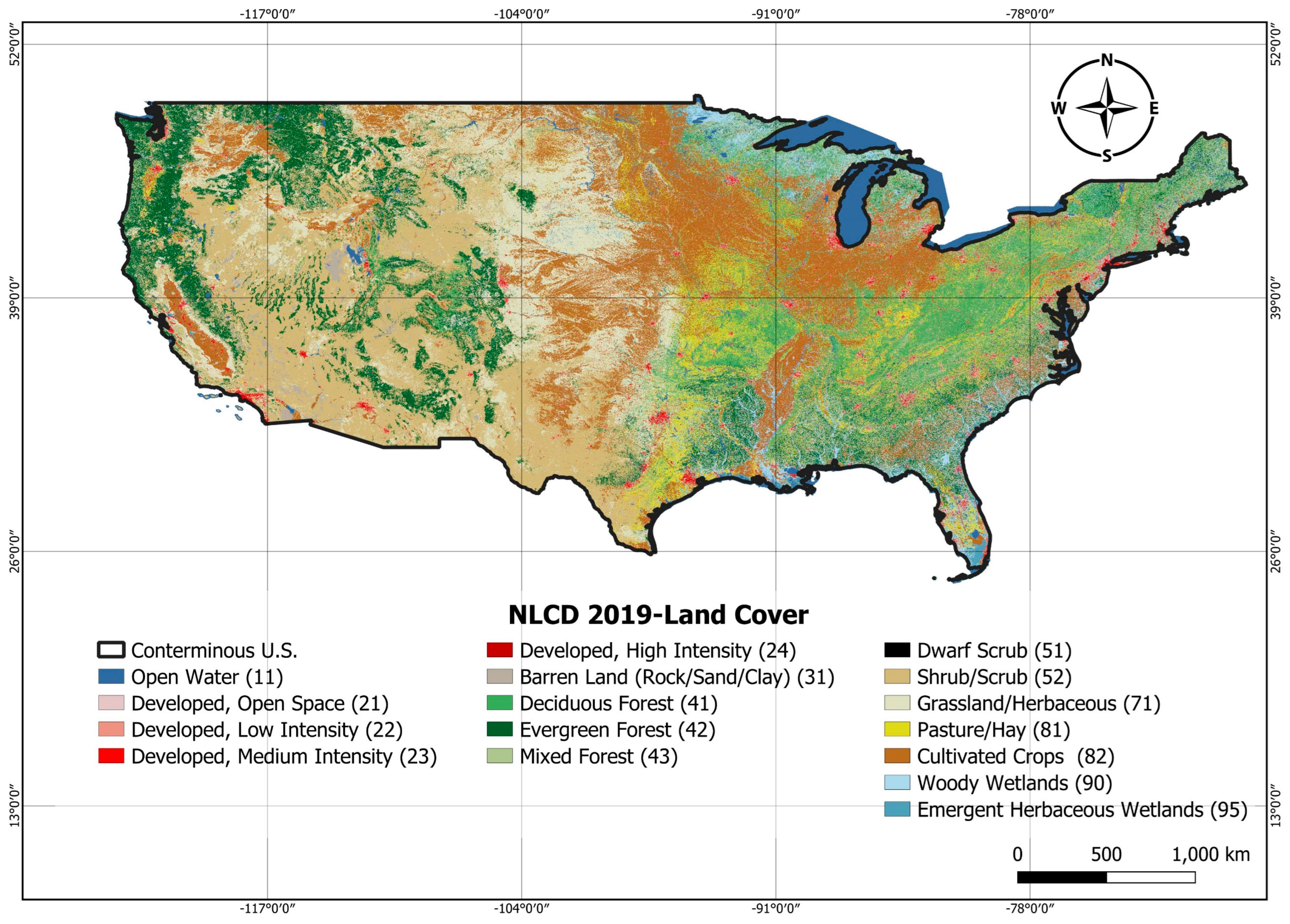
The National Land Cover Database (ver. 2.0) was released in June 2021. A new version of the NLCD dataset (under the name NLCD 2019) was released by the USGS with a resolution of 30 m [31]. The NLCD 2019 design aims to provide innovative, consistent, and robust methodologies for the production of a land-cover change database from 2001 to 2019 at 2–3 years intervals land-cover with 16 different classes as shown in Figure 1. Table 1 illustrates the land-cover detailed topologies description for the NLCD 2019 map [31].
Landsat imagery for the NLCD 2019 dataset was processed based on an integrated training process that depends on different sources in addition to temporally and spatially integrated land-cover analysis and modelling [32].
2.2. Environmental Systems Research Institute Land Use/Land CoverDatabase (LULC 2020-ESRI)
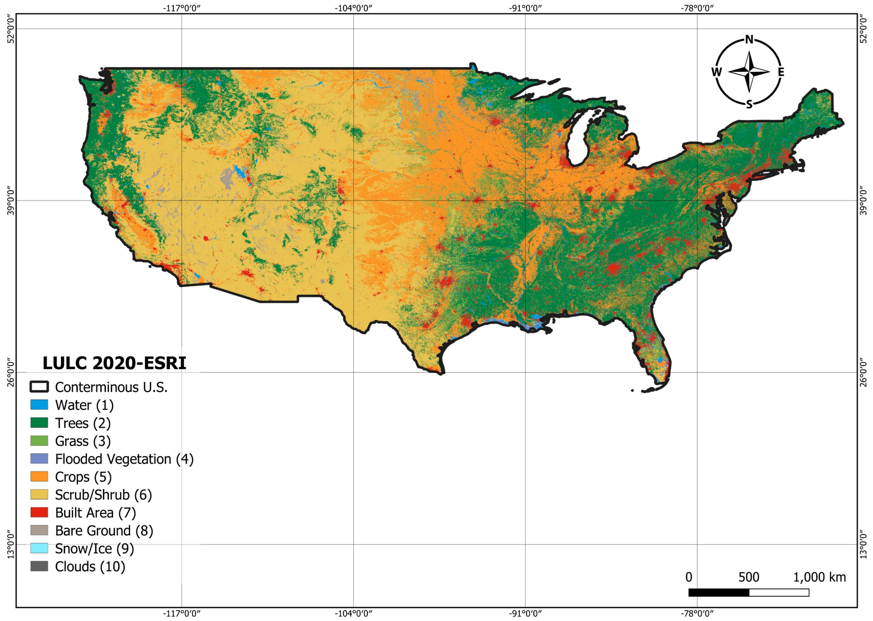
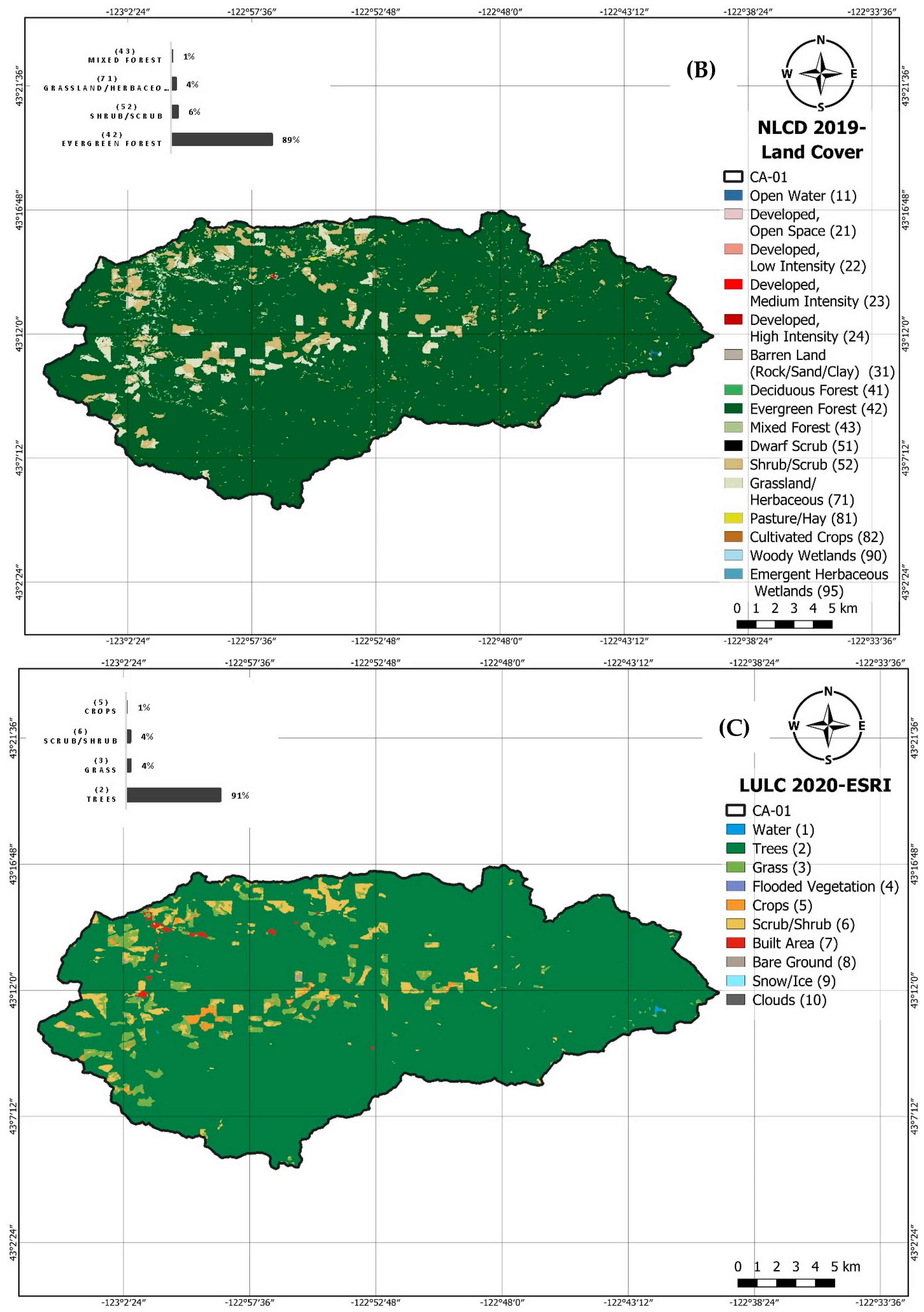
The Sentinel-2 satellites are excellent candidates for LULC mapping due to their high spatial and temporal resolution. In addition, advances in deep learning and scalable cloud-based computing now provide the analysis capability required to unlock the value in global satellite imagery observations. Based on a novel, very large dataset of over 5 billion human-labeled Sentinel-2 pixels, the Environmental Systems Research Institute (ESRI) developed and deployed a deep learning segmentation model to create a global cover LULC map with a resolution of 10 m. This dataset is called LULC 2020-ESRI [33]. The global LULC 2020 map has been clipped with the conterminous U.S. boundary as shown in Figure 2 for comparison purposes with NLCD 2019. The LULC 2020 map is classified into ten classes as shown in Table 2. It should be noted that, however, the LULC 2020-ESRI has finer resolution compared to the NLCD 2019, but with fewer land-cover categories, making it a coarser dataset.
2.3. Rainfall and Peak Flow Data
For calibration and validation of the hydrodynamic model, trusted measurements and data for rainfall and corresponding runoff are needed in the current study. Rainfall and runoff data were extracted from USGS-StreamStats v4.10.1 [37] and National Oceanic and Atmospheric Administration (NOAA) Atlas 14 [38]. USGS-StreamStats v4.10.1 is a map-based web application (https://streamstats.usgs.gov/ss/ accessed on 5 May 2022.) that provides analytical tools that are useful for water-resource planning and management and engineering purposes. It is developed by the U.S. Geological Survey (USGS); the primary purpose of StreamStats is to provide estimates of stream-flow statistics for user-selected ungauged sites on streams and USGS stream gauges [37]. Stream-flow statistics can be computed from available data at USGS stream gauges depending on the type of data collected at the stations. However, stream-flow statistics are often needed at ungauged sites, where no stream-flow data are available to determine the statistics [37].
NOAA Atlas 14 provides a point-and-click interface that contains precipitation estimates with associated frequency (return periods) for the United States and is supported by additional information such as seasonality and temporal distribution. This Atlas 14 precipitation frequency estimate is intended as the official documentation and associated information for the United States [38].
2.4. 2D Hydrodynamic Modeling (HEC-RAS 2D)
HEC-RAS (v. 6.2) simulates unsteady flow for 1D and 2D modeling. The 2D modeling simulates flow hydraulics over the floodplain and river channel. The model discretizes the analysis domain into computational cells to represent elevations and calculate flow parameters along a horizontal plane from a computational cell into an adjacent cell.
HEC-RAS 2D calculates the flow rate and water-surface elevation for adjacent cells using cell-boundary hydraulic properties [39]. The model solves the 2D Shallow Water Equations (SWE) or Diffusion Wave Equations (DWE) with the application of an implicit finite volume solution algorithm. SWE is derived using continuity and momentum equations, and DWE is an approximation of SWE obtained by neglecting the inertial terms of the momentum equations [40]. Within the HEC-RAS, DWE is the default method since it improves modeling performance in terms of minimizing the simulation time.
The most recent advancement in HEC-RAS [41] was the simulation of 2D unsteady flows in response to rain-on-grid model input, accounting for soil infiltration and other losses with spatial variation of roughness values (Manning’s roughness coefficients). Water depth and velocity variability in floodplain and channel environments can be quantified using HEC-RAS 2D rain-on-grid simulations [41]. The HEC-RAS model implements the Soil Conservation Service–Curve Number SCS–CN method (the most widely used method) to account for the losses in rainfall depth and then simulates the direct runoff values at each grid cell of the model domain [42,43].
2.5. Manning’s Roughness Coefficients by Land Classification
There are several references to be used by users to assign Manning’s roughness values (n) as reference values. For example, in Chow’s book “open channel hydraulics” (1959), there is a large collection of Manning’s roughness values for floodplains and main streams [14]. HEC-RAS Mapper User’s Manual also suggested Manning’s values for the NLCD as reference values to be used in floodplain and stream analysis [5] as shown in Table 3.
2.6. Research Methodology
The research methodology consists of two parts. The first part is data preparation, statistical analysis, and accuracy assessment. The second part is validating and studying the effects of implementing the research findings in flood modeling applications.
2.6.1. Part 1: Data Preparation, Accuracy Assessment, and Roughness Analysis
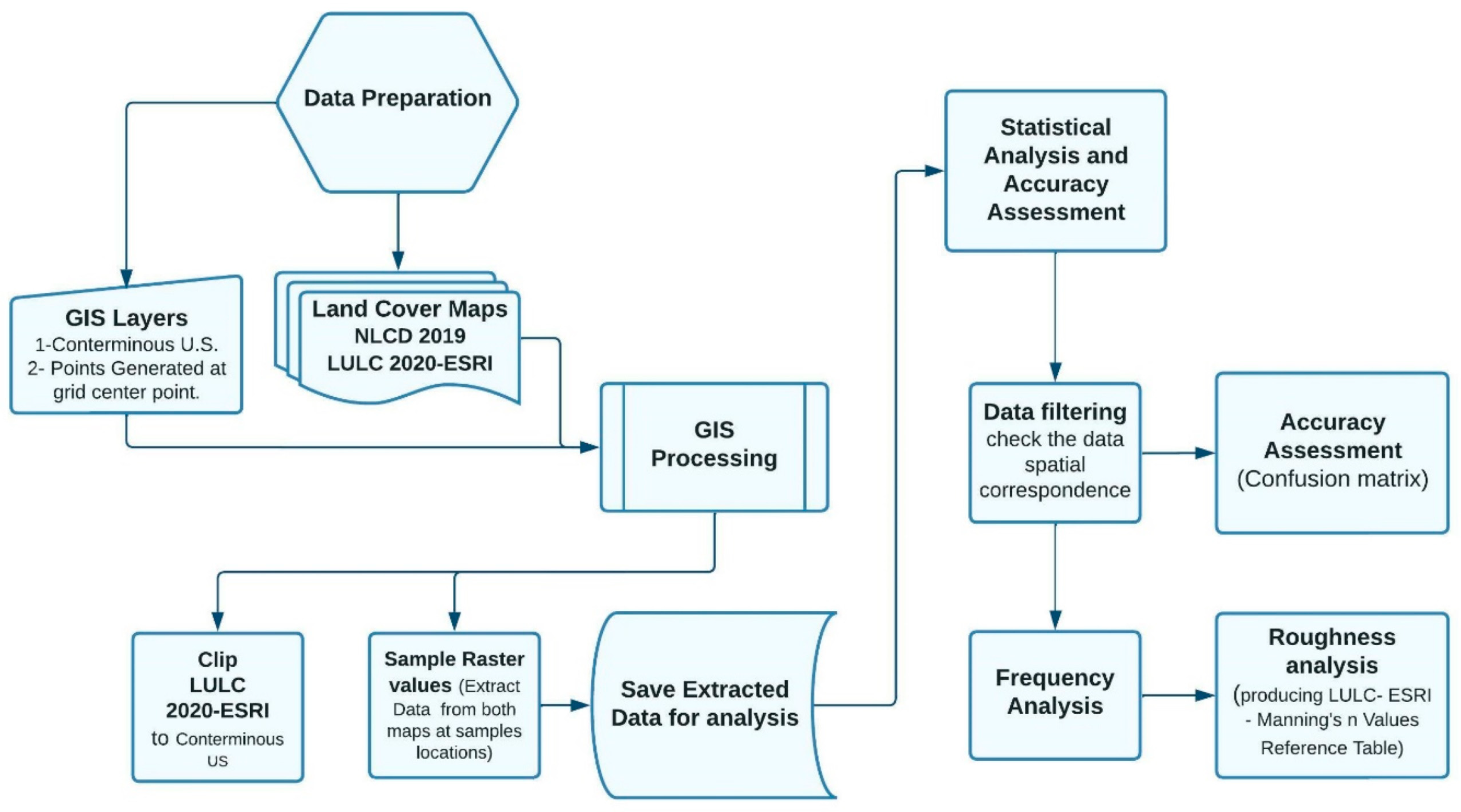
To assess how accurately the global LULC 2020-ESRI spatially compared to the reference NLDC 2019 land-use data, both LULC 2020-ESRI and NLDC 2019 land-use data inside the conterminous United States boundary was first extracted. Therefore, the conterminous United States total area (8,080,464.3 km2) was discretized into equal areas of about 15 km2, generating a total of 548,117 sample points to be exported at each grid centroid to quantify the spatial correspondence between both products (i.e., LULC 2020-ESRI data and NLCD 2019 datasets). The raster value extraction tool was used to extract the values from both datasets. Accuracy assessment is a very demanding requirement for such LULC classification [32,34]. The 548,117 data samples of LULC 2020-ESRI were then subjected to accuracy assessment by generating classification confusion matrices and accuracy reports. The confusion matrix method [34,44] was conducted to calculate the quantitative correspondence relationship between the LULC 2020-ESRI and the NLCD 2019 maps, which contain trusted high-accuracy data. The confusion matrix generates the following results: overall accuracy, accuracy for each class, and percentage of error.
Based on the reference Manning’s roughness values mentioned in Table 3, the appropriate Manning’s roughness values need to be assigned to each land-cover category for the global LULC 2020-ESRI land-use map. A detailed per-class statistical/frequency analysis was performed. A flow chart in Figure 3 describes this part of the conducted methodology. The next section shows the used statistical averaging methods which were applied to develop the proposed Manning’s roughness values:
- A.
- Average of the most frequent in-class data (Average Manning’s Value)
For the selected class and based on the histogram/class, the average of Manning’s roughness (n) for the most repeated categories corresponding to the class under study was considered to represent the class roughness value as shown in Equation (1). In this method the frequency of each repeated category was not taken into consideration.
where:
- Average Manning’s value per LULC 2020-ESRI class.
- : Manning’s value for the repeated class N from NLCD 2019 standard values.
- : Number of most repeated categories.
- B.
- Weighted Average of the most frequent in-class data (W. A. Manning’s Value):
For the same selected categories and considering the frequency, the weighted average of Manning’s n value was considered to be selected to represent the class as in Equation (2).
where:
- : Weighted Average Manning’s value per LULC 2020-ESRI class.
- : Manning’s value for the repeated class N from NLCD 2019 standard values.
- : Frequency of points having value of class N from NLCD 2019 standard values.
- : Summation of Frequencies (f)
2.6.2. Part 2: Calibration/Validation of the Developed Roughness Maps Using Flood Modeling Application
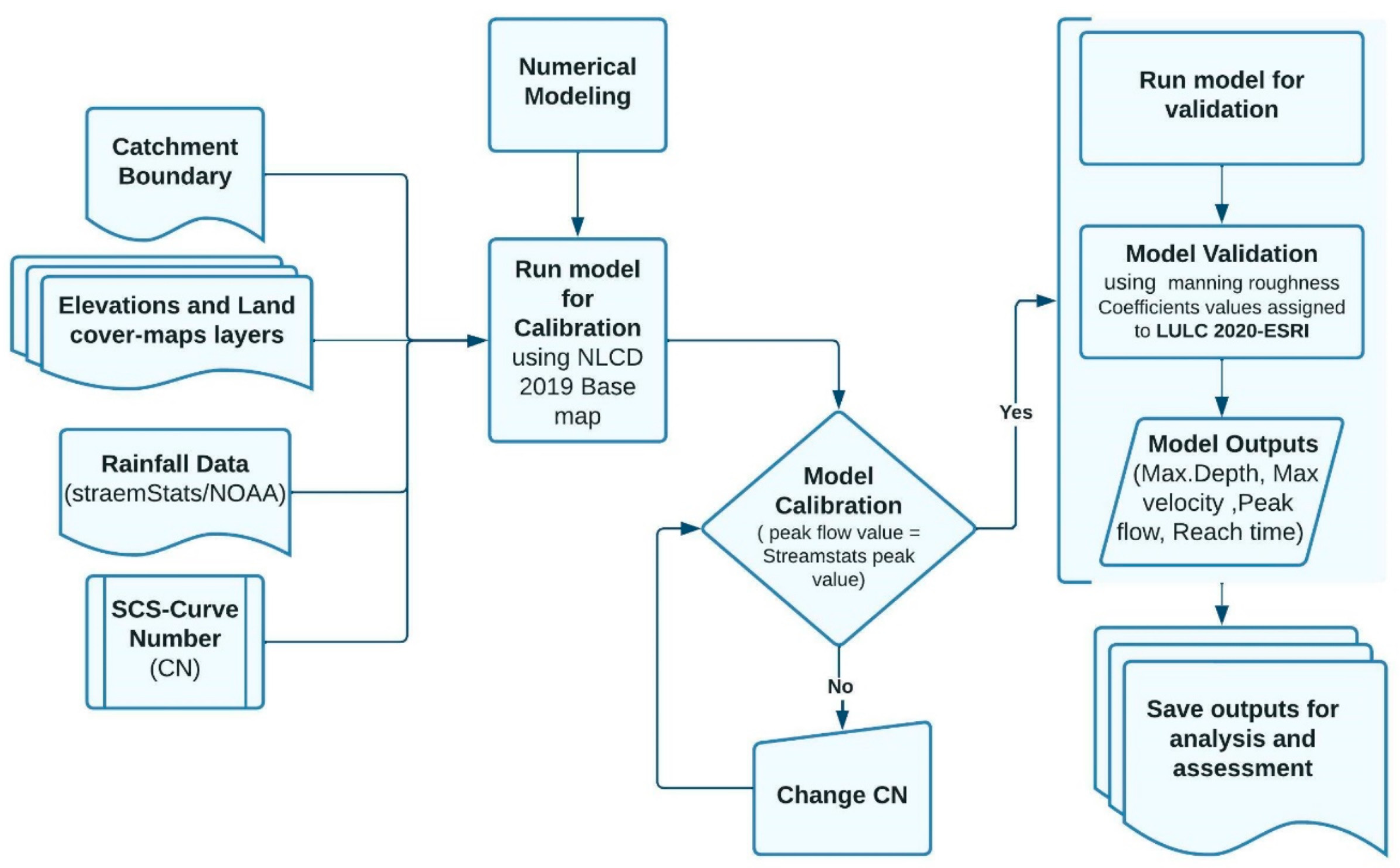
To calibrate and verify the methodology of generating the proposed Manning’s roughness values, nine catchment areas were randomly selected based on the data available on StreamStats. A spatial Manning’s roughness layer for each catchment was generated based on the proposed values from the assessment step using HEC-RAS 2D (v. 6.2) [13,21]. A Digital Elevation Model (DEM) was downloaded for each catchment area location with the best available resolution from U.S. national map imagery [45]. The nine rain-on-grid simulation models have been calibrated by implementing the NLCD 2019 map as a first step, using the reference Manning’s roughness values provided in the HEC-RAS Mapper manual [5]. Rainfall data and peak flow values were obtained from StreamStats. The NOAA Atlas 14 database was used to obtain the missing rainfall data that have no values in StreamStats. Then model scenario runs were performed using the LULC 2020-ESRI with the proposed Manning’s roughness values to be compared with the model scenario runs using the NLCD 2019. A flow chart in Figure 4 describes this part of the conducted methodology.
3. Results
3.1. Data Analysis
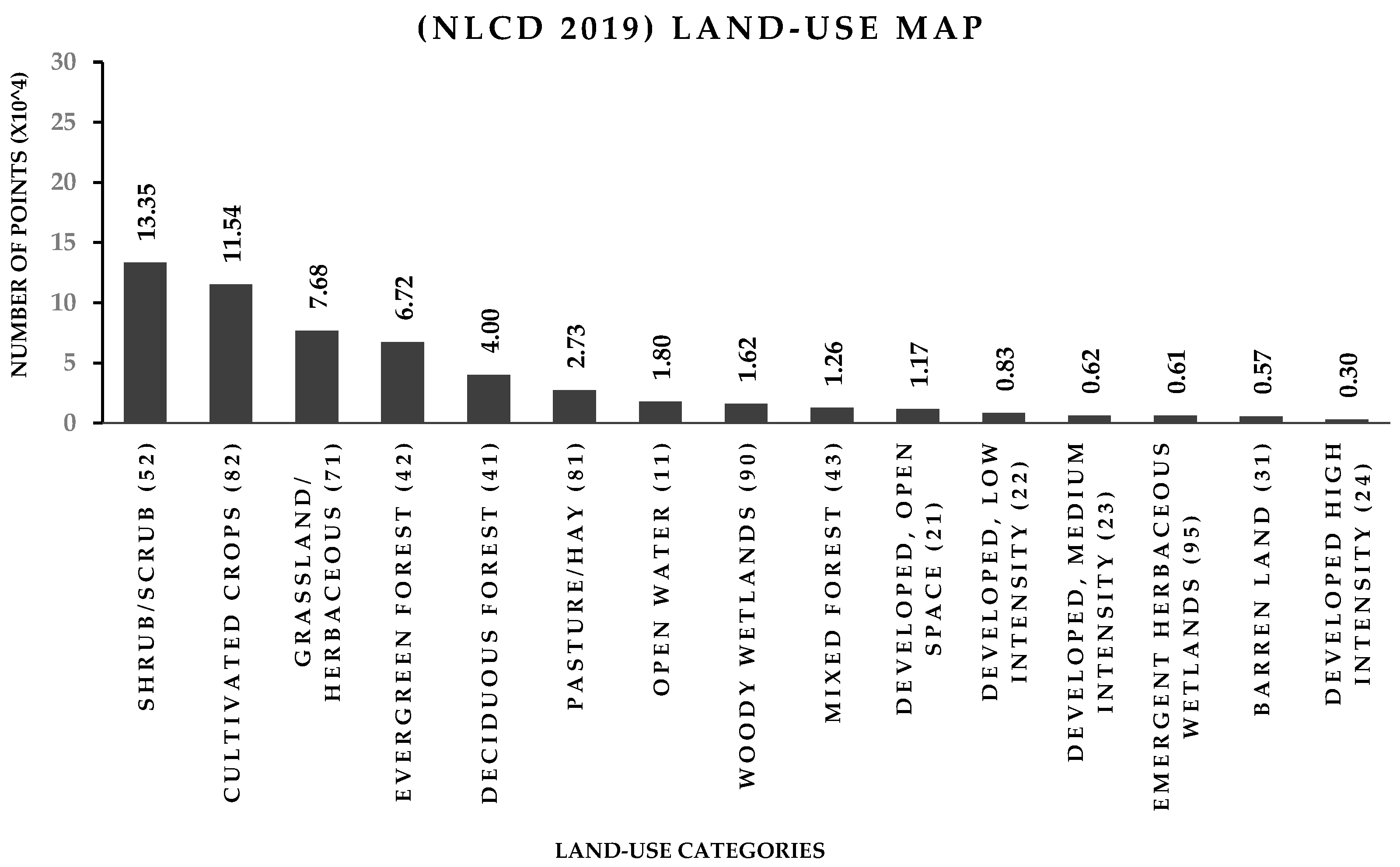
The samples’ frequency analysis from both products (i.e., NLCD 2019 and LULC 2020-ESRI) shows an acceptable spatial correspondence between the two products. Figure 5 shows the total number of repetitions (frequency) in each topology class for the NLCD 2019 map, and Figure 6 shows the same analysis of the LULC 2020-ESRI map.
The previous analysis showed that shrub land has the most repetition values derived from both maps, followed by cultivated croplands. The lowest repetition was snow, and clouds were not found in the study samples. However, there seems to be some confusion in the rest of the classes. This may be due to the smaller number of LULC 2020-ESRI classes compared to NLCD 2019, aggregating more than one class from the corresponding reference map NLCD 2019.
3.2. Accuracy Assessment (Confusion Matrix)
To quantify the cross-correspondence between both maps, a detailed analysis was conducted for each class separately after excluding the snow and cloud classes. LULC 2020-ESRI land-use map data were assessed using a confusion matrix using NLCD 2019 land-use map data as well-trusted and high-accuracy data [32,34]. Table 4 shows the accuracy assessment results.
The accuracy for each class topology was calculated considering the percentage of the truly captured points to the total number of samples for each class. For example, the first column in Table 4 represents the LULC 2020-ESRI Water (1) category corresponding to class Open Water (11) in the NLCD 2019 map. This study found about 17,175 truly captured points out of 18,379 total points in this class; this was reflected in the 93% accuracy and 17% error in simulating this class. The overall accuracy represents the summation of all true values percentage in all classes to the total number of samples.
3.3. Surface Roughness Analysis (Manning’s Roughness(n) Values)
The appropriate Manning’s roughness values for each topology in LULC 2020-ESRI can be assigned considering the detailed definition of the classes in Table 2. It can be concluded that the LULC 2020-ESRI classes Water, Bare ground, Scrub/shrub, Crops, and Flooded vegetation approximately match the NLCD classes open water, barren land, shrub/scrub, cultivated crops, and emergent herbaceous wetlands, respectively, based on the outcomes of the conducted analysis in the accuracy assessment section. Accordingly, Manning’s roughness values for these classes can be assigned easily using the corresponding classes in the reference map (NLCD 2019) referring to the values in Table 3.
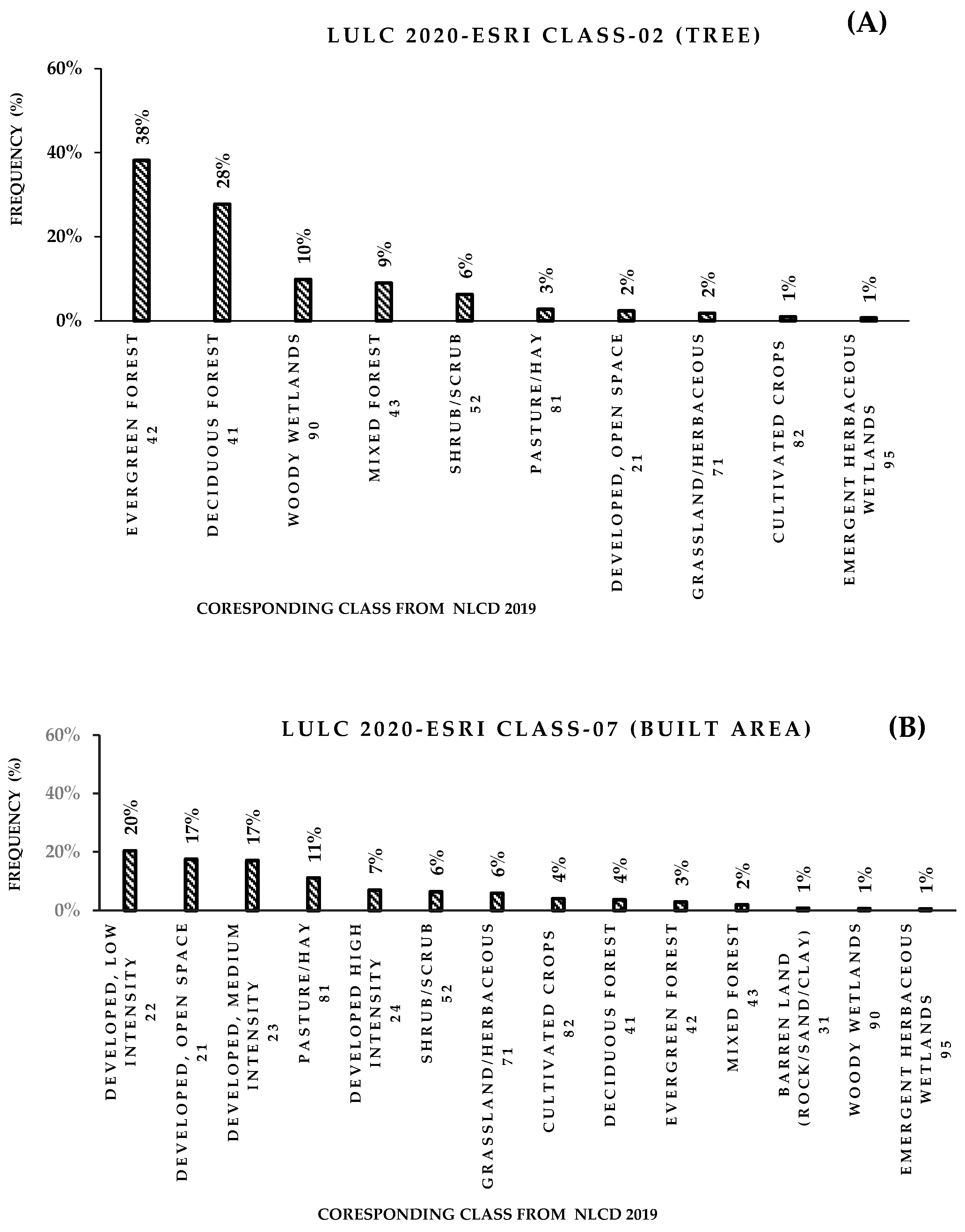
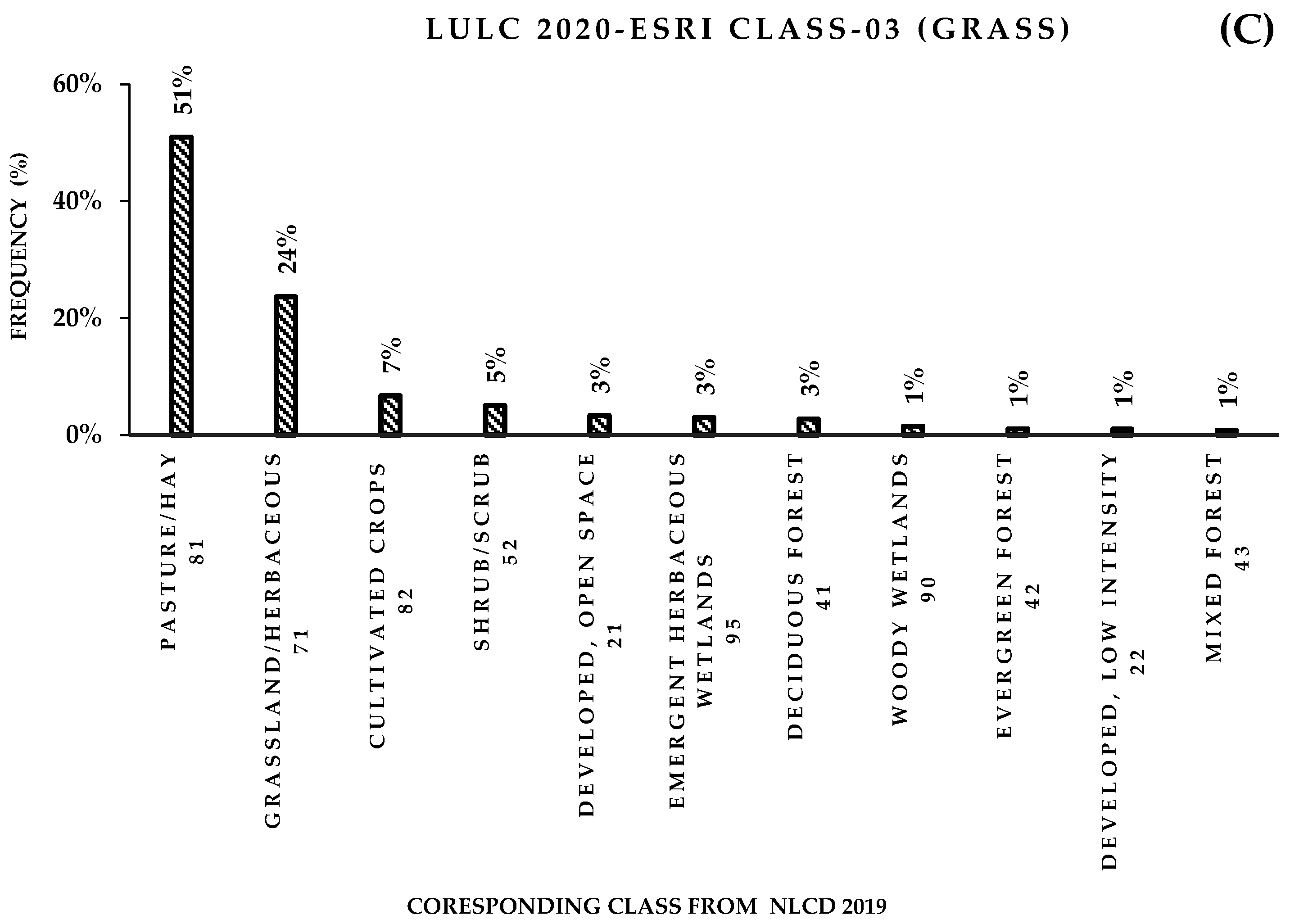
It is worth noting that each biased classes in LULC 2020-ESRI (trees, grass, and built area) aggregates more than one class from the reference map, NLCD 2019. Detailed frequency analysis was conducted to ensure an efficient representation and identification for each class individually. Figure 7 shows the mentioned classes and the frequency analysis for spatially corresponding classes in the reference map. Further detailed statistical analysis described was used to assign the appropriate Manning’s roughness values for the three mentioned biased classes, applying both averaging and weighted averaging methods (refer to Section 2).
3.4. Hydrodynamic Modeling
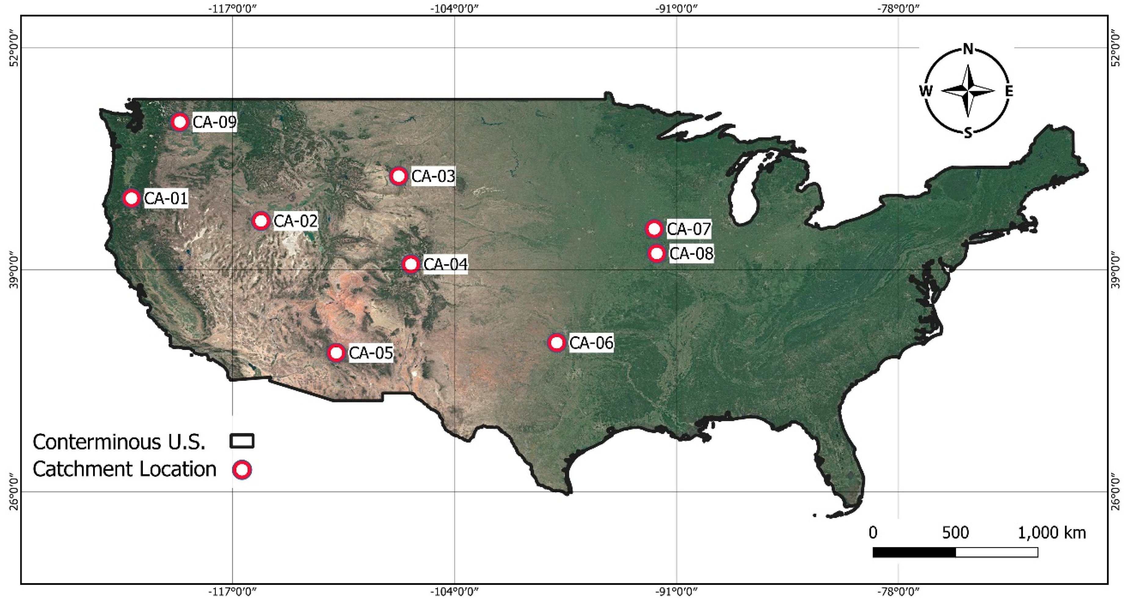
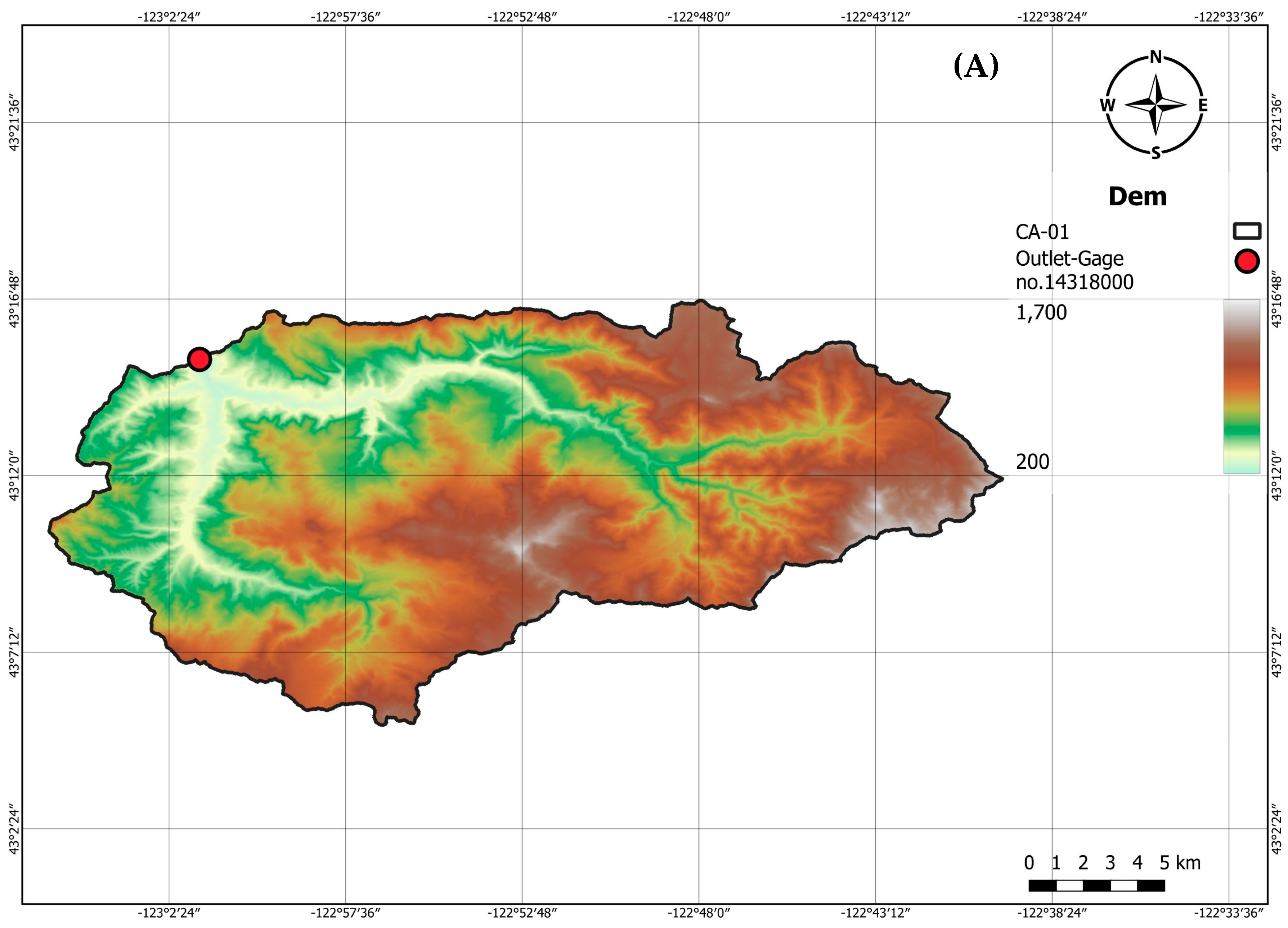
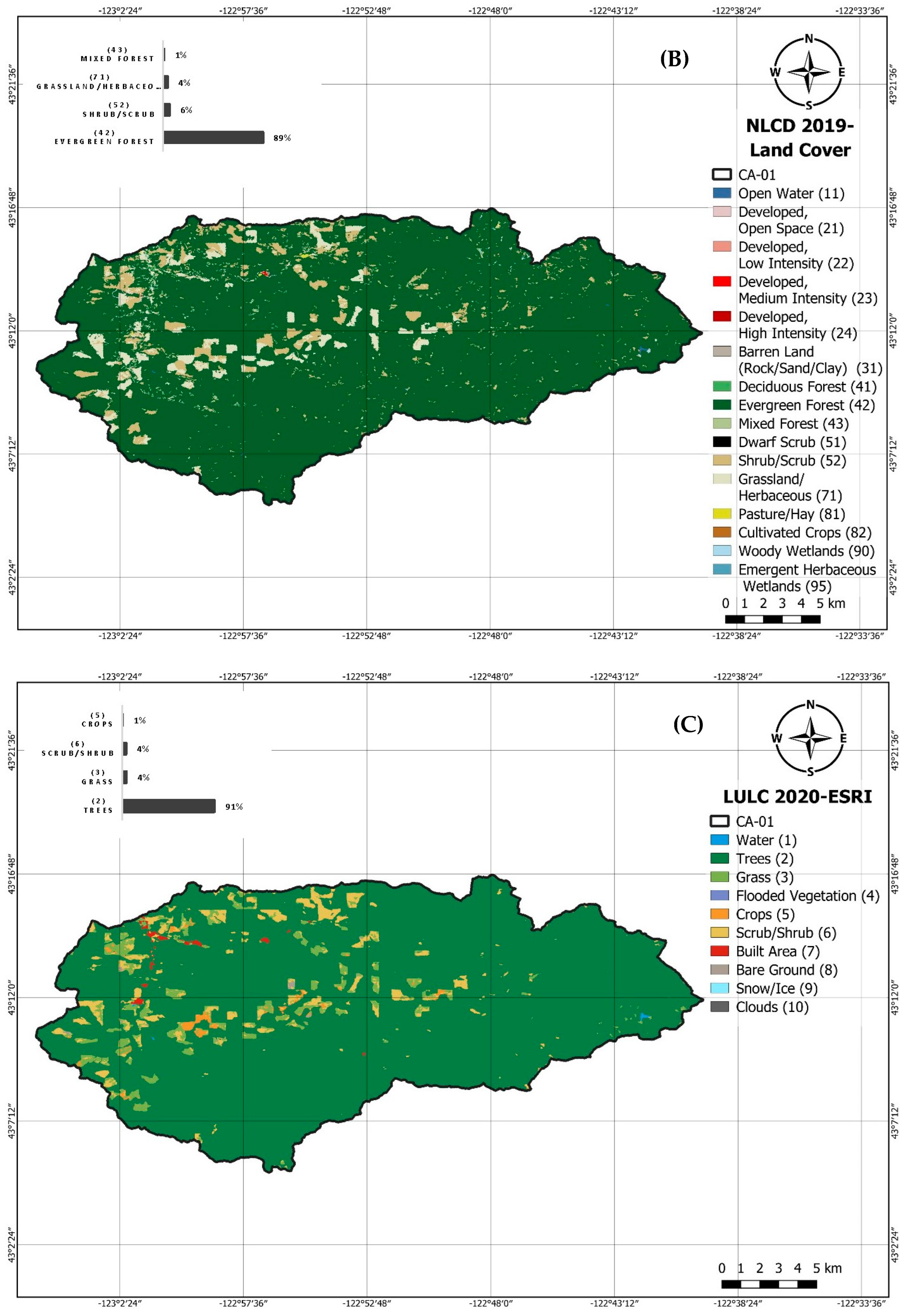
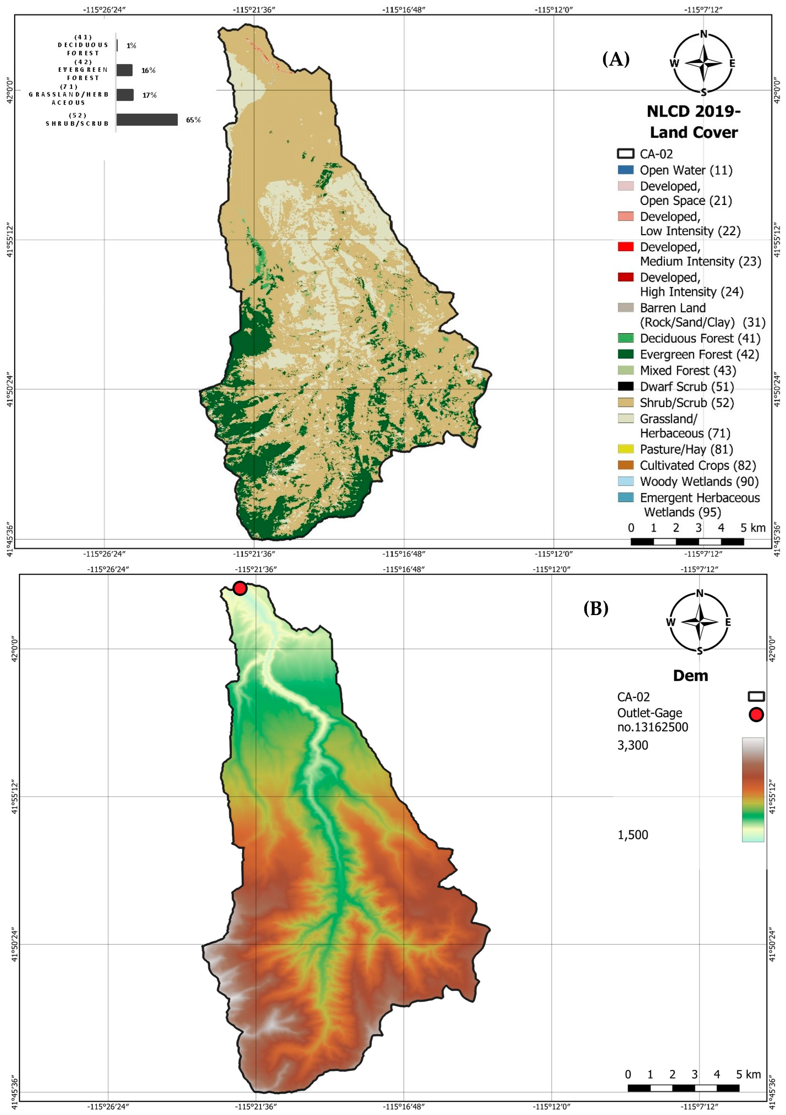
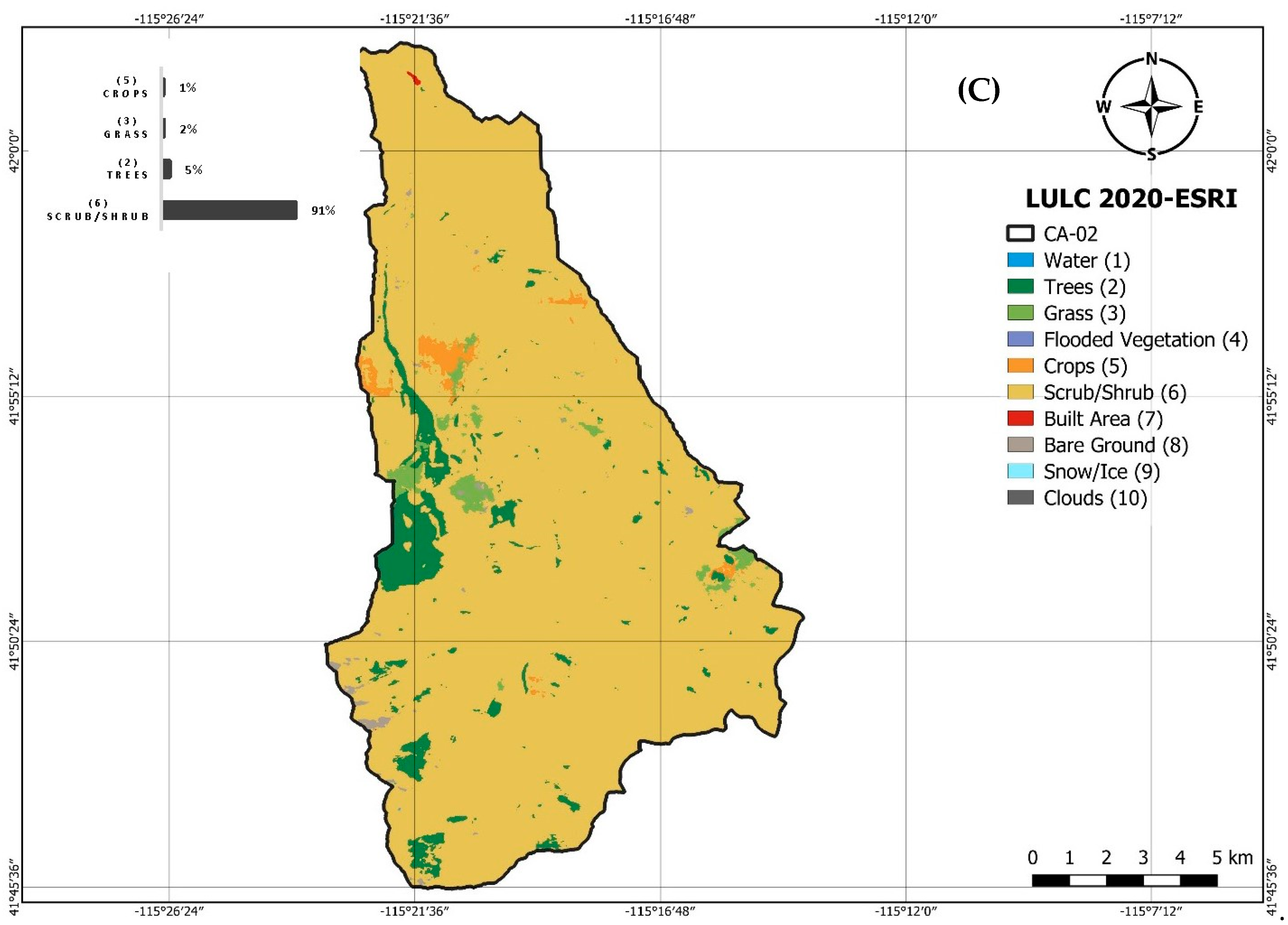
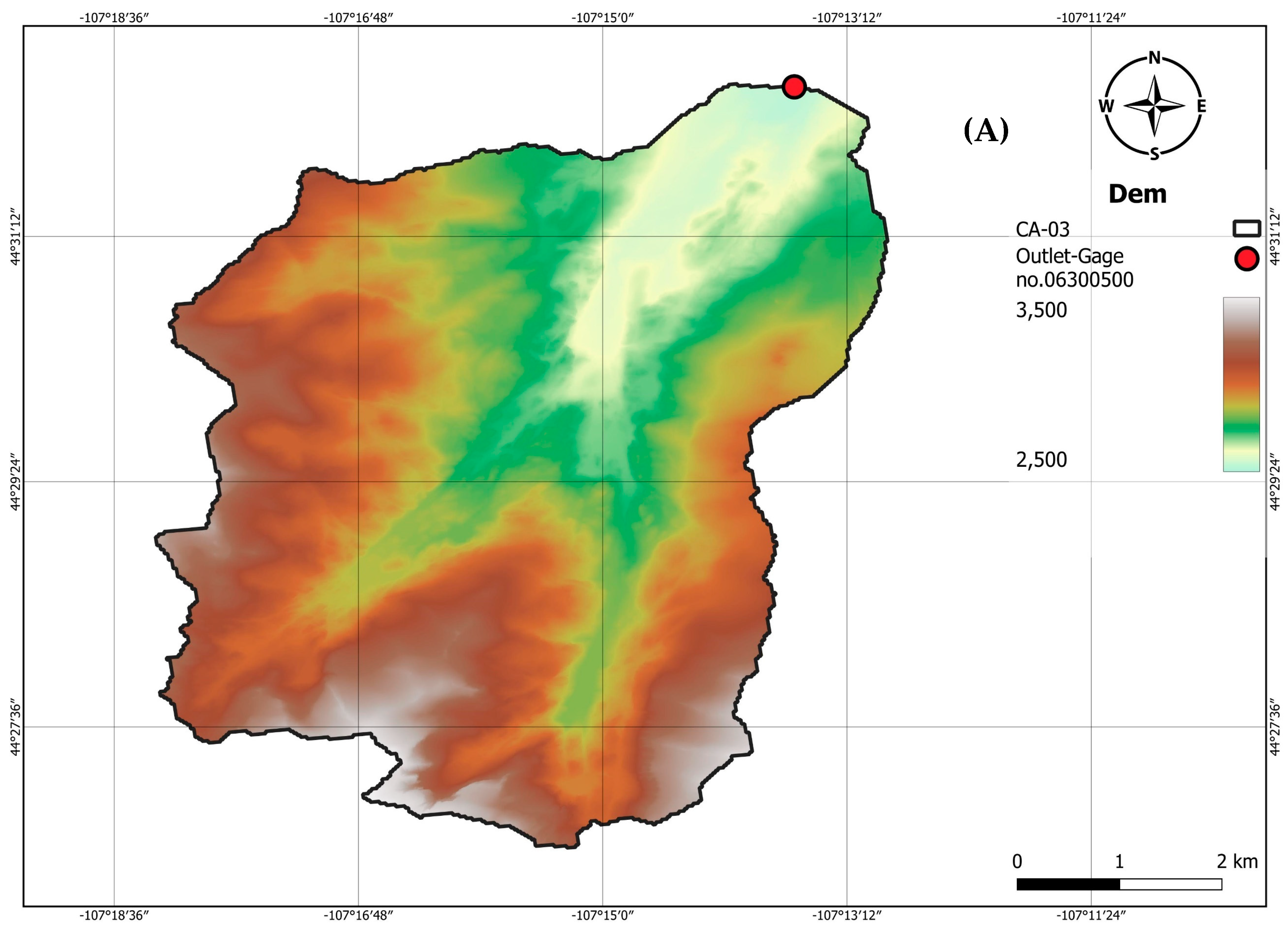
Rain-On-Grid (ROG) simulations for the modeling of 2D unsteady flows and floodplain parameters in response to precipitation input were implemented in HEC-RAS V.6.2 software to validate the performance of the presented methodology [13,46]. Nine catchments were randomly selected based on the data availability in StreamStats and NOAA Atlas 14. Figure 9 shows the location of the selected catchments in the conterminous United States. Rainfall and runoff flow data were extracted from StreamStats and NOAA Atlas 14, respectively. The selected catchments have varied areas (from 8 km2 to 460 km2) with a mixed land-use cover. Table 6 shows the selected catchment locations and areas. Figure A1, Figure A2, Figure A3, Figure A4, Figure A5, Figure A6, Figure A7, Figure A8 and Figure A9 in Appendix A show the DEM and land-use land-cover maps with the spatial distribution for these catchments. Figure 10 shows DEM and land-use maps for each class for catchment CA-01 as an example.
3.4.1. Calibrating HEC-RAS 2D Models
Model calibration and validation based on water level and flow observations are necessary to determine any model’s ability to reproduce reality [47]. The HEC-RAS (v.6.2) model was calibrated using the calibration data in Table 7 and as mentioned in the methodology section. The main objective of this step was to assess the effect of implementing the developed Manning’s roughness values on the modeling results’ accuracy and quantify the derived errors and uncertainty. The collected rainfall data and corresponding runoff values at different return periods were divided into two sets, one for calibration (2-year return period) and the other for validation (100-year return period), as presented in Table 7. All rainfall and runoff data were extracted from StreamStats, except the 100-year return period rainfall data for some of the catchments, which were extracted from NOAA Atlas 14. All catchments’ data were found in both data sources (USGS-StreamStats and NOAA Atlas 14), but no rainfall data were found covering CA-01, CA-02, or CA-03 in the 100-year return period.
Using the collected data in Table 7 and implementing the DEM and projected land-use layers in Appendix A, the HEC-RAS 2D ROG modeling was utilized to solve for the flow peaks, times to the peak, maximum depths, and velocity values over the catchment area. This model was built using the NLCD 2019 along with Manning’s roughness guidance values in Table 3.
Calibration was conducted using the mentioned methodology with the variation of the Soil Conservation Service Curve Number (SCSCN). The initial SCS–CN was selected based on the soil type and land use land cover in the catchment and according to the suggested values based on urban hydrology for small watersheds (TR-55) [48]. The calibrated Curve Number (CN) for each catchment in order to catch the observed peak flow for a 2-year return period is illustrated in Table 7.
The calibrated results using NLCD 2019 maps were used as a baseline case. Table 8 shows acceptable accuracy in simulating the peak flow value corresponding to the distributed rain-on-grid in the baseline case. Then the proposed Manning’s values either for the average or weighted average method for LULS-2020-ESRI were used in the hydrodynamic modelling and compared with the baseline case for calibration. HEC-RAS 2D calibration model results for the selected catchments (e.g., flow hydrographs at catchments outlets and maximum depths over the catchment areas) are shown in Appendix B; Figure A10, Figure A11 and Figure A12.
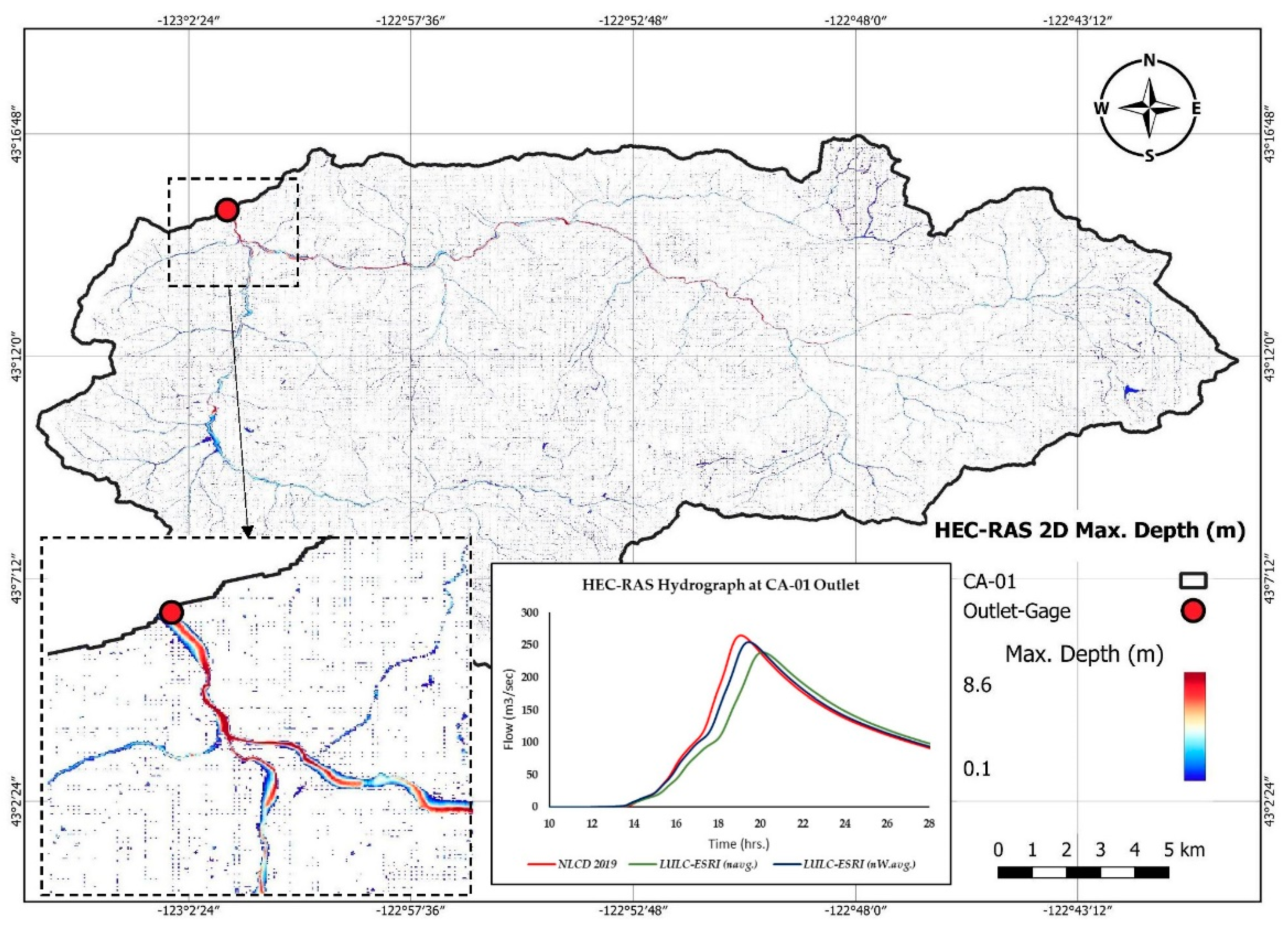
The 2D flood-modeling results are expressed in flow hydrographs corresponding to the base map and the global LULC map along with the proposed Manning’s value and the flood maximum depths over the catchment area. Figure 11 shows the HEC-RAS 2D results for the first catchment (CA-01) as an example using DEM and land-cover maps illustrated in Figure 10, and the calibration results for other catchments are shown in Appendix B. The accuracy of the developed Manning’s roughness was tested by applying the statistical performance indicators to the set of simulated peak flow values, maximum depths, and maximum velocities. Table 8 shows the calibration results and values of Root Mean Squared Error (RMSE) and Mean Absolute Error (MAE) [47]. Calibrating was conducted using the data in Table 7 for a 2-year return period. Calibration results were extracted, tabulated, and tested using the statistical performance indicators considering NLCD 2019 results as a reference for peak flow, depth, and velocity values over the study area (baseline case).
3.4.2. Validation Results: Testing the LULC 2020-ESRI Maps along with the Proposed Roughness Values
To verify the results, the same analysis conducted on LULC 2020-ESRI maps in the calibration process was repeated but using a 100-year return period. The results of the hydrodynamic model using the NLCD 2019 dataset for a 100-year return period and using the calibrated CN numbers were used as the baseline case for the validation process of LULC 2020-ESRI. The results show an acceptable agreement with accurate capturing of the peak flow and flood parameters (depth and velocity). Table 9 shows the simulation analysis results for the validation simulations. The same analysis was conducted in the calibration stage and the errors were calculated relative to the StreamStats observations, showing a very good performance and relatively low magnitude of errors.
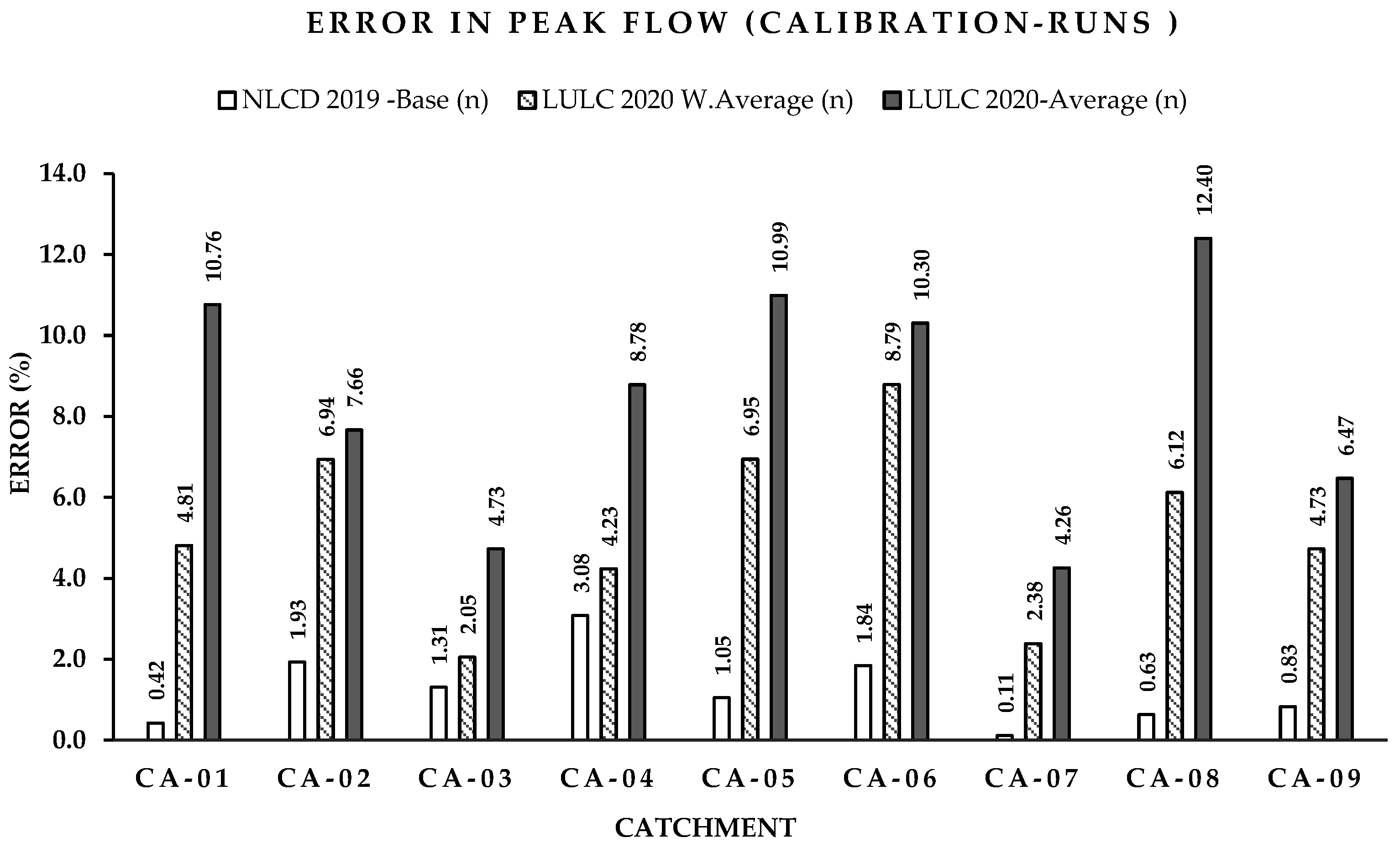
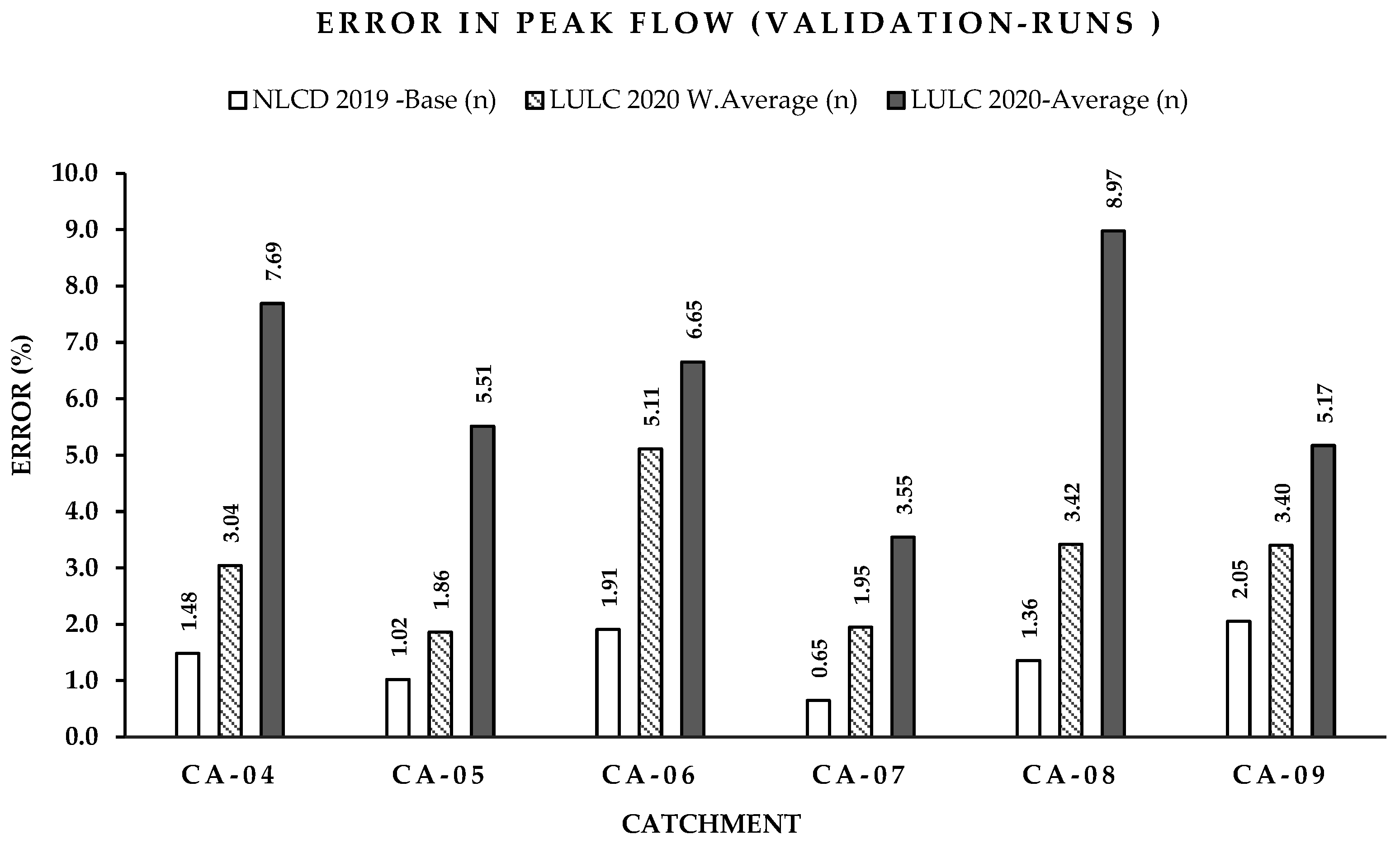
It should be noted that the errors in peak-flow capturing and the driven errors in depths and velocities were relatively reduced with the increase in the rainfall return period. Accordingly, the 24 hr rainfall depth comparison between the analysis results was summarized and presented in bar charts. Figure 12 and Figure 13 show a comparison between the driven errors in peak-flow capturing for both calibration and validation sets of simulations, respectively.
The analysis shows a severe reduction in the driven errors from the Manning’s roughness values generated from the weighted average (nw.avg) compared to the one generated from the average method (navg). As an example from the first catchment (CA-01) results in Figure 12, the derived error using NLCD 2019 maps was 0.42% as a baseline case (compared with StreamStats v4.10.1 values) and about 10.7% when implementing ESRI maps (compared with NLCD 2019 results) when using average Manning’s n values, and the error was reduced to 4.8% when implementing the global maps along with weighted average (nw.avg) values.
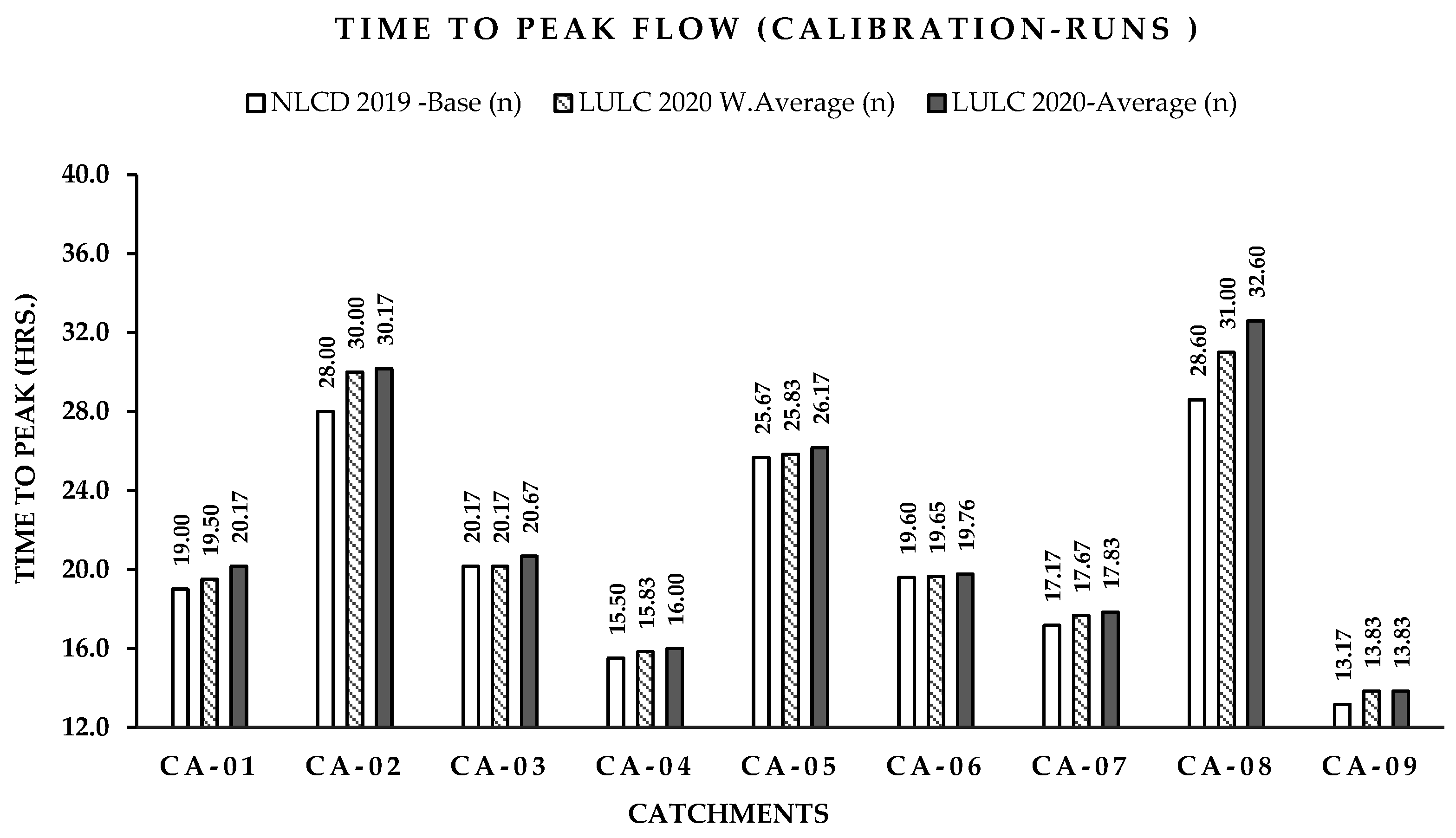
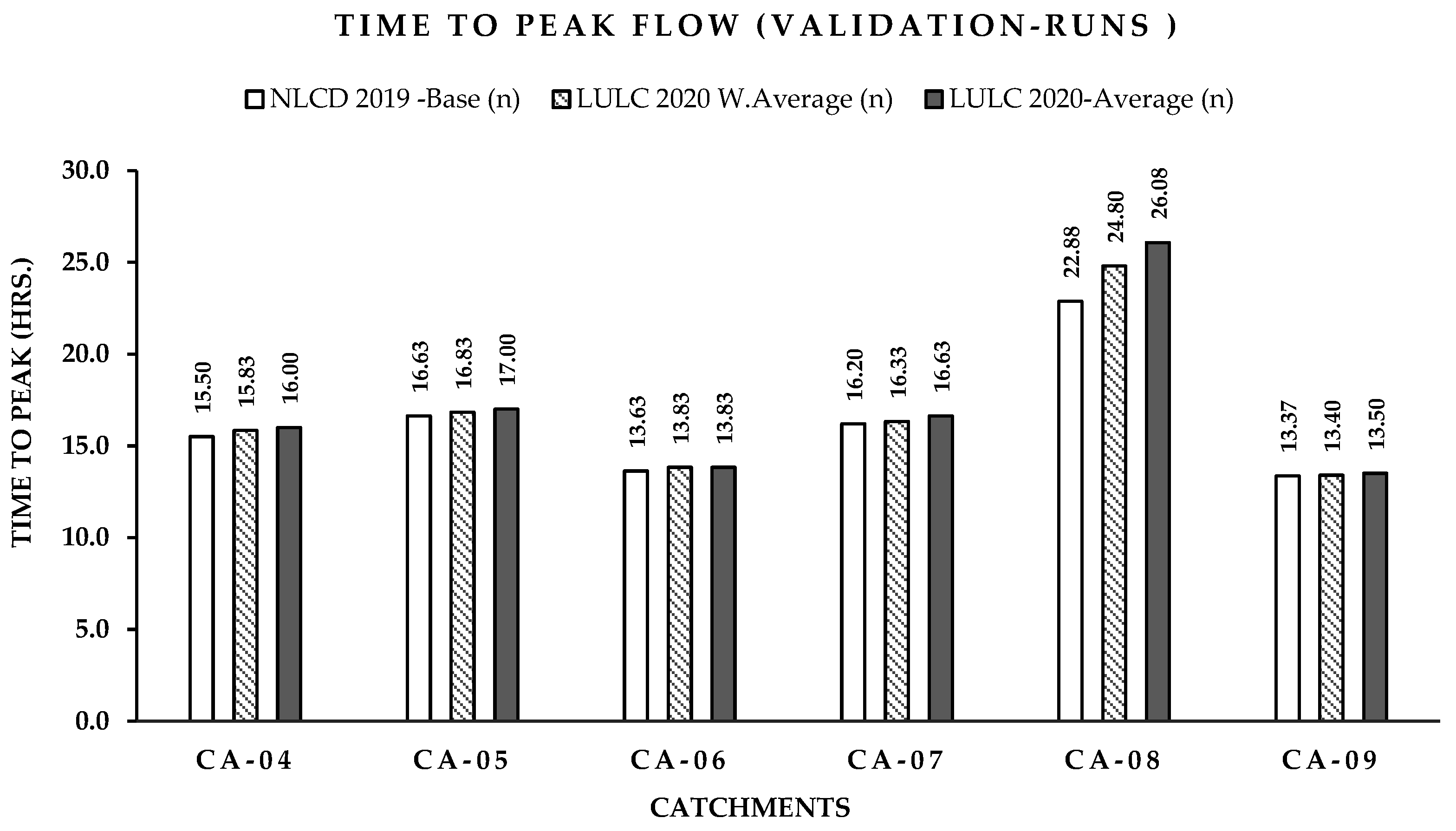
From the analysis results, Table 8 and Table 9, it was found that the time to peak using LULC 2020-ESRI with weighted average Manning’s roughness values (nw.avg) was always closer to the base line case, compared to those values using proposed average Manning’s roughness values (navg) in both the calibration and validation cases. Figure 14 and Figure 15 show the time to the peak comparison using the implemented maps for the calibration and validation simulations, respectively.
4. Discussion
Based on the statistical analysis results, it is obvious that the data from NLCD 2019 is denser and more accurate where it can catch the observed peak flow with an error ranging from 0.42% to a maximum of 3.08% for calibration and validation processes, respectively. These error rates were lower in the long return period (100-year validation process) than for the short return period (2-years calibration process) (Table 8 and Table 9). However, the NLCD 2019 is only available for the conterminous U.S. and it cannot be used for global coverage. Due to the main advantage of global coverage for the LULC 2020-ESRI map, there was a need to make full use of the NLCD 2019 dataset to enhance the accuracy and propose Manning’s roughness values for the LULC 2020-ESRI dataset.
A confusion matrix was prepared in order to compare between the two datasets (NLCD 2019 and LULC 2020-ESRI), and cross-correspondence between both maps was achieved based on the full description for each class in the two datasets illustrated in Table 2 and Table 3. Based on the results shown in Table 4, the “water” class was the most accurately mapped class (93%), followed by “trees” (86%), “crops” (81%), “built area” (77%), and “Grass” (71%). Lowest accuracy was obtained for the classes “Bare Ground” (57%), “Scrub/shrub lands” (56%), and “Flooded vegetation” (54%). The comparison results show an overall accuracy of around 72% with an error of 28% for the LULC 2020-ESRI map compared to the NLCD 2019 land-use map as a reference map (Table 4). From the recent publications regarding the global-coverage maps’ accuracy assessment referenced to ground truth with a mapping unit of 250 m2 data [35], it was found that the overall accuracy of LULC 2020-ESRI maps had the highest value of 75%, which is consistent with the results from the current study.
Table 5 illustrates the most matching classes between the two datasets; most of the classes in LULC 2020-ESRI were matched with only one class in the NLCD 2019 dataset, except for only three biased classes: grass, trees, and built area. Two statistical techniques, average and weighted average methods, were used to detect the proposed Manning’s roughness values for biased classes.
Based on the HEC-RAS 2D ROG analysis, implementing the proposed LULC 2020ESRI Manning’s roughness values for both average and weighted average methods (Table 8), it was concluded that the weighted average values (nw.avg) in all simulations showed relatively less time to peak and accurate peak-flow values. The average error in the peak flow is 5.22% (2.0% min. to 8.8% max.) for weighted average values (nw.avg) compared to 8.5% (4.4% min. to 12.4% max.) when using the LULC 2020-ESRI map with average Manning’s roughness values (navg) (Table 8). Appendix B shows flow hydrographs at the catchments’ outlets using the implemented maps.
Using both of the statistical performance measures mean square error (RMSE) and mean absolute error (MAE), the HEC-RAS computational results were extracted and GIS tools were used to calculate floodplain inundated maximum depths and velocities. It has been concluded from the results in Table 8 that the LULC 2020-ESRI maps using weighted average Manning’s roughness values (nw.avg) in all simulations give lower error values with an overall value (RMSEdepth) of 2.7 cm, compared to 3.72 cm when using average Manning’s roughness (n) values, and an MAEdepth of 5.32 cm, compared to 7.75 cm when using average Manning’s roughness values (navg). The same analysis was repeated to measure the errors (RMSE and MAE) in the velocity simulation, and it was found to confirm the same performance.
Testing the same catchments’ responses to the ROG HEC-RAS model using the validation dataset with 100-year 24 h rainfall (Table 9) reveals that during high return periods, the error in capturing the peak value was reduced to an average of 3.13% when using weighted average Manning’s roughness values (nw.avg), compared to 6.62% when using average Manning’s roughness values (navg). Also, during the validation process, the error values in the water depth RMSE and MAE were with an average value of 3.8 cm and 4.2 cm, respectively, when using weighted average Manning’s roughness values (nw.avg), compared to 4.7 cm and 8.1 cm, respectively, when using average Manning’s roughness values (navg). The same analysis was repeated to measure the errors (RMSE and MAE) in the velocity simulation, and it was found to confirm the same performance.
One of the main outputs of the current study is the generated new base/reference for Manning’s roughness values for each class in the global land-use maps LULC 2020-ESRI. The generated maps using these Manning’s roughness values have been tested and confirmed to drive a low magnitude of error with an acceptable accuracy in both calibration and validation processes. Recommended Manning’s roughness values to be compatible with the global LULC 2020-ESRI maps are presented in Table 10.
5. Conclusions
The more crucial input data for flood modeling are land use and land cover, translated into corresponding Manning’s roughness values to effectively replicate the water depth and velocity. Currently, there are two available datasets for land cover and land use, NLCD 2019 and LULC 2020-ESRI. In contrast to the LULC 2020-ESRI dataset, which has worldwide coverage but no reference to Manning’s roughness values, the NLCD 2019 dataset has national coverage but with available references to Manning’s roughness values for each class derived from prior studies. The main conclusions of this study can be summarized as follows:
- A confusion matrix was used to compare the two publicly available land-use and land-cover datasets for a total of 548,117 sample points in the conterminous United States.
- During the calibration and validation procedures using the HEC-RAS 2D model, the NLCD 2019 dataset was evaluated using the measured peak flows for nine catchments in the conterminous United States with an accepted error in peak flow of 0.42% to a maximum of 3.08%.
- The LULC 2020-ESRI dataset can be used to depict the global coverage with an overall accuracy of 72% compared to the NLCD 2019 dataset, which is consistent with recent scientific studies.
- Compared to the average method, the weighted average approach is the most effective way to determine Manning’s roughness values for the LULC 2020-ESRI dataset.
- Manning’s roughness values were suggested (see Table 10) for the classes in LULC 2020-ESRI to be used as standard reference values for the 2D flood-modeling procedure.
- The suggested Manning’s roughness values for the LULC 2020-ESRI dataset were calibrated and validated against the NLCD 2019 dataset using the HEC-RAS 2D model, and their accuracy was deemed acceptable. The overall RMSE in depth was 2.7 cm, the MAE in depth was 5.32 cm, and the accuracy of the computed peak flow value had an average error of 5.22% (2.0% min. to 8.8% max.).
- Using LULC 2020-ESRI and the suggested Manning’s roughness values (nw.avg) results in lower-magnitude errors for long return periods than for short return periods.
- This work should be updated and modified for any new release of LULC-ESRI or NLCD land use/land cover.
Finally, the proposed Manning’s roughness values for LULC 2020-ESRI in this research can be used as a reference and implemented efficiently in the distributed 2D hydrodynamic models.
6. Patents
Standard Manning’s Roughness (n) values corresponding to each class compatible with LULC-ESRI maps to be implemented in flood distributed 2D modeling.
Author Contributions
Conceptualization, M.S., M.M.M. and H.G.R.; methodology, M.S., M.M.M. and H.G.R.; formal analysis, M.S. and M.M.M.; writing—original draft preparation, M.S.; writing—review and editing, M.M.M. and H.G.R.; supervision, M.M.M. and H.G.R. All authors have read and agreed to the published version of the manuscript.
Funding
This research received no external funding.
Data Availability Statement
Data used in this research are available online as follows; LULC 2020-ESRI is available online at https://www.arcgis.com/apps/instant/media/index.html?appid=fc92d38533d440078f17678ebc20e8e2 accessed on 1 March 2022, NLCD 2019 is available online at https://www.usgs.gov/data/national-land-cover-database-nlcd-2019-products accessed on 1 March 2022, 3DEP DEM -Products is available online at https://www.usgs.gov/3d-elevation-program/about-3dep-products-services accessed on 1 March 2022, rainfall data—NOAA Atlas 14 is available online at https://hdsc.nws.noaa.gov/hdsc/pfds/pfds_map_cont.html accessed on 1 May 2022, and rainfall and flow data—StreamStats v4.10.1 is available online at https://streamstats.usgs.gov/ss/ accessed on 1 May 2022.
Conflicts of Interest
The authors declare no conflict of interest.
Appendix A
Figure A1.
DEM and land-use maps for Catchment CA-01 (A) DEM, (B) NLCD 2019 land-use map, (C) LULC 2020-ESRI land-use map.
Figure A1.
DEM and land-use maps for Catchment CA-01 (A) DEM, (B) NLCD 2019 land-use map, (C) LULC 2020-ESRI land-use map.


.
Figure A2.
DEM and land-use maps for Catchment CA-02 (A) DEM, (B) NLCD 2019 land-use map, (C) LULC 2020-ESRI land-use map.
Figure A2.
DEM and land-use maps for Catchment CA-02 (A) DEM, (B) NLCD 2019 land-use map, (C) LULC 2020-ESRI land-use map.


Figure A3.
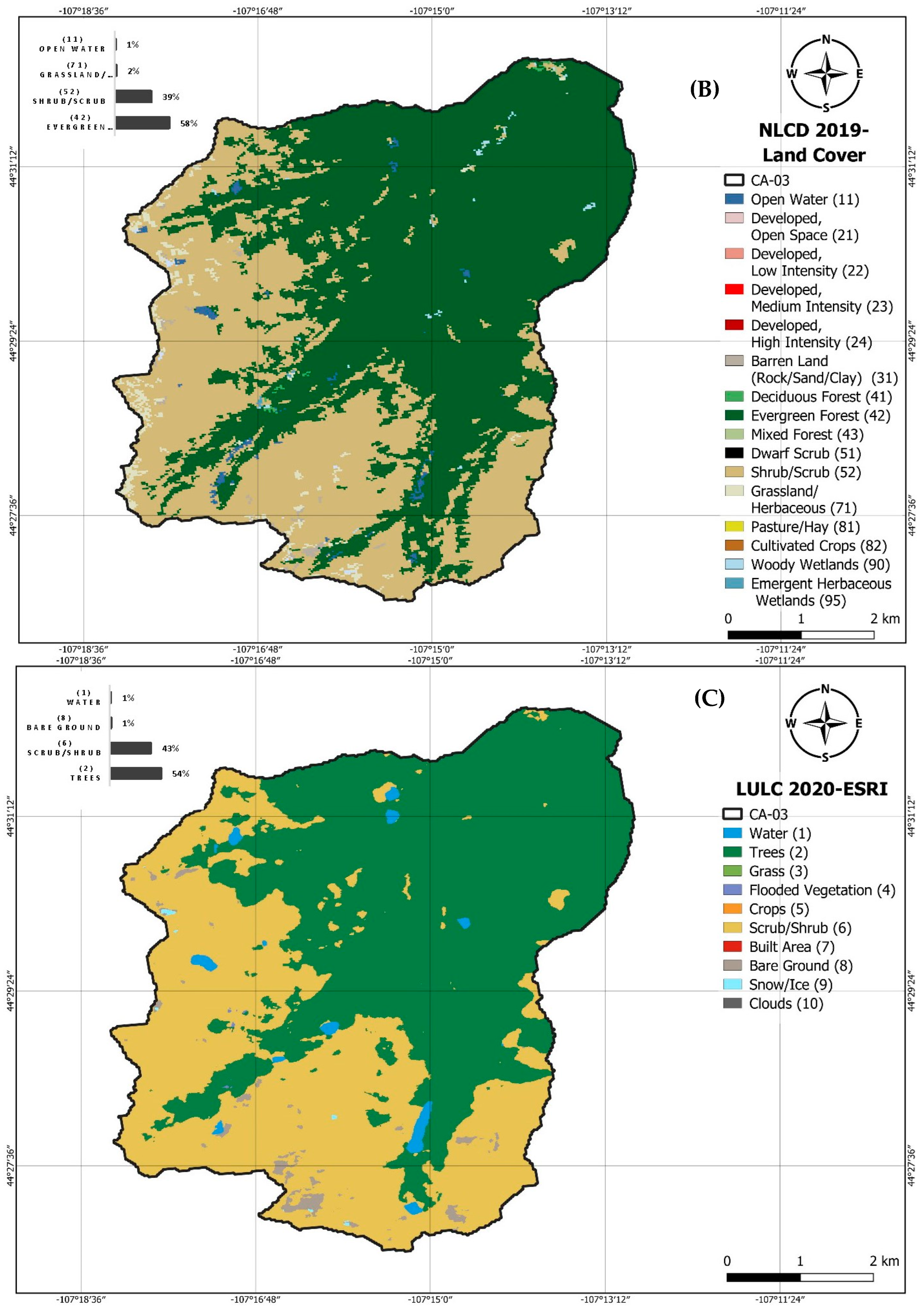
DEM and land-use maps for Catchment CA-03 (A) DEM, (B) NLCD 2019 land-use map, (C) LULC 2020-ESRI land-use map.
Figure A3.
DEM and land-use maps for Catchment CA-03 (A) DEM, (B) NLCD 2019 land-use map, (C) LULC 2020-ESRI land-use map.


Figure A4.
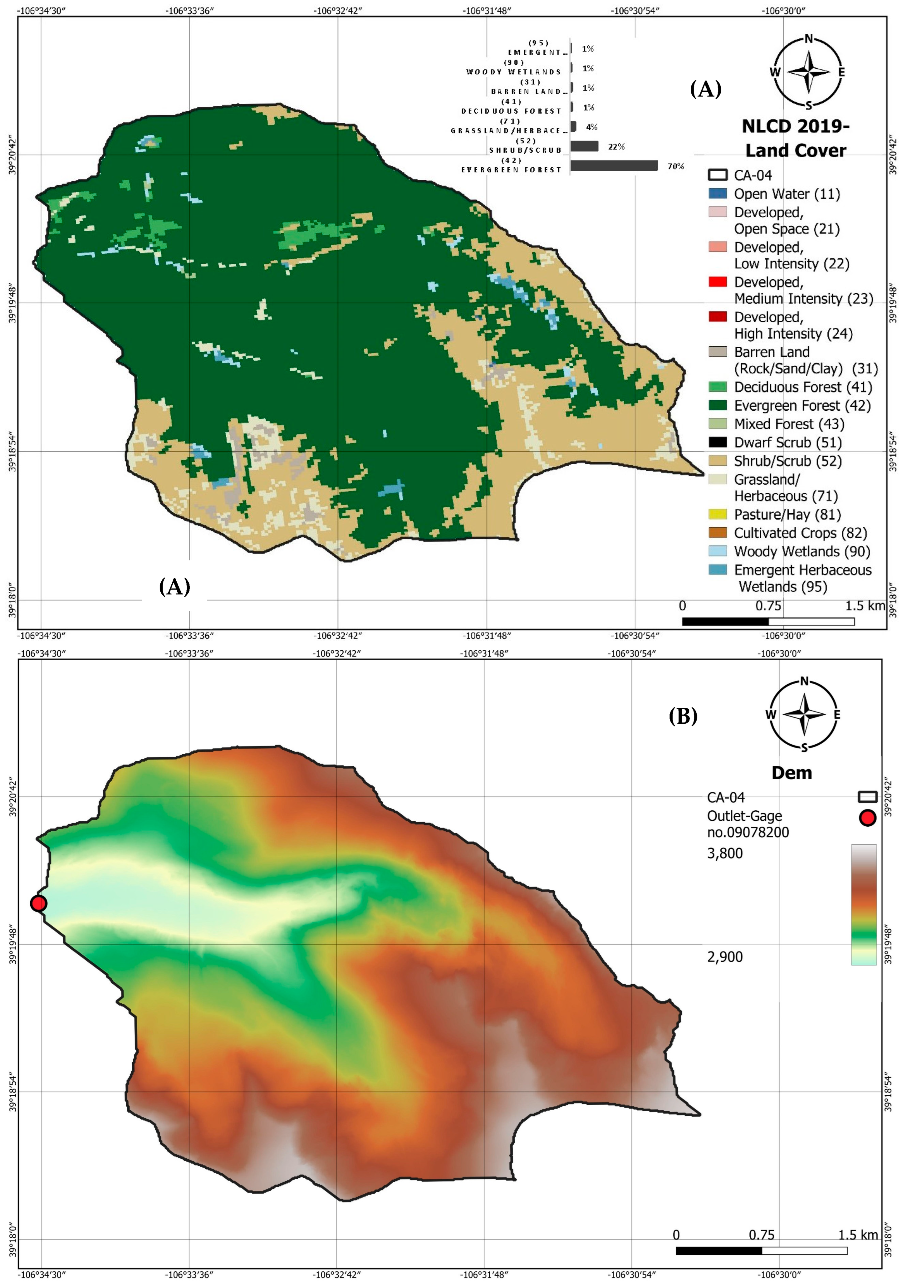
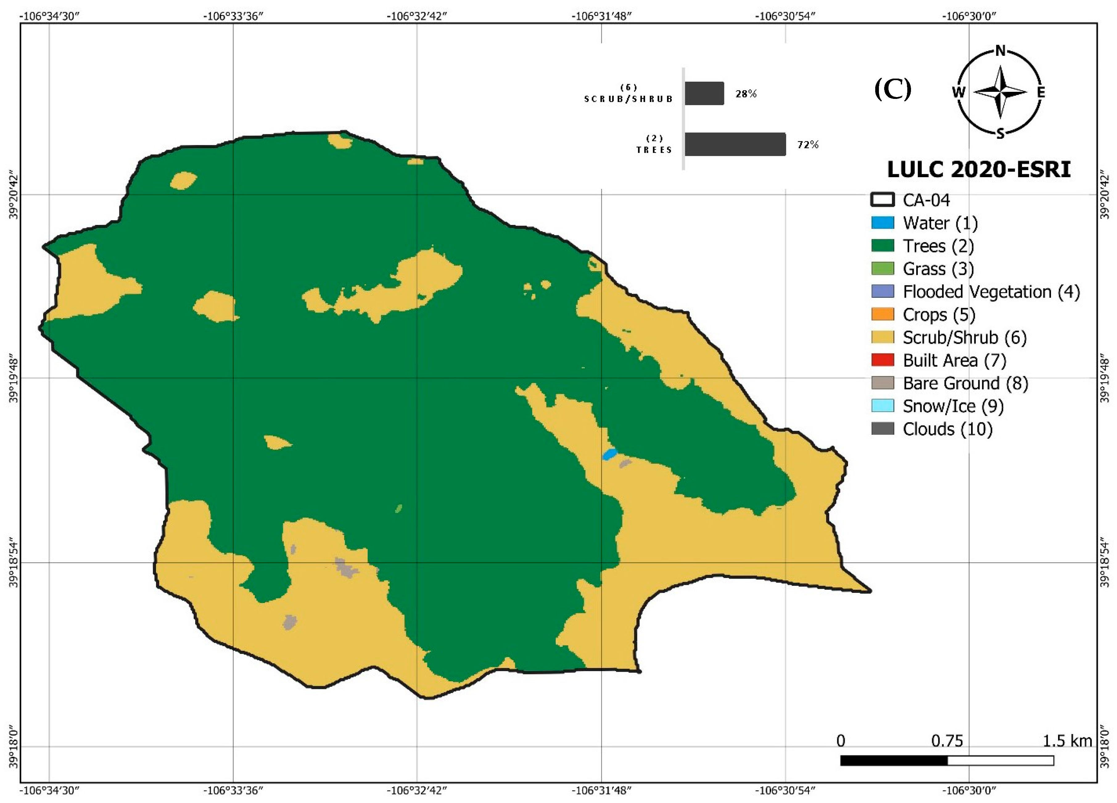
DEM and land-use maps for Catchment CA-04 (A) DEM, (B) NLCD 2019 land-use map, (C) LULC 2020-ESRI land-use map.
Figure A4.
DEM and land-use maps for Catchment CA-04 (A) DEM, (B) NLCD 2019 land-use map, (C) LULC 2020-ESRI land-use map.


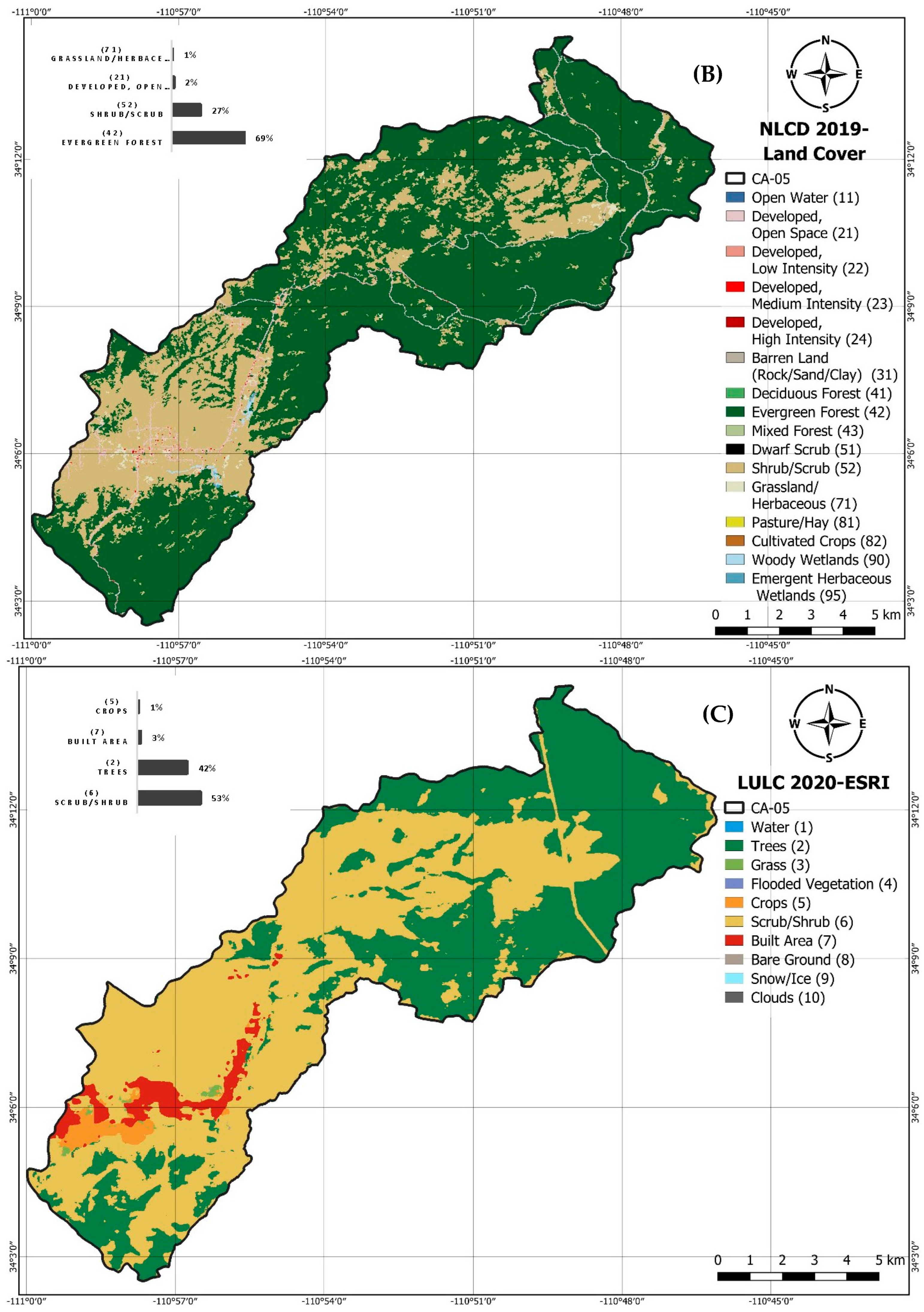
Figure A5.
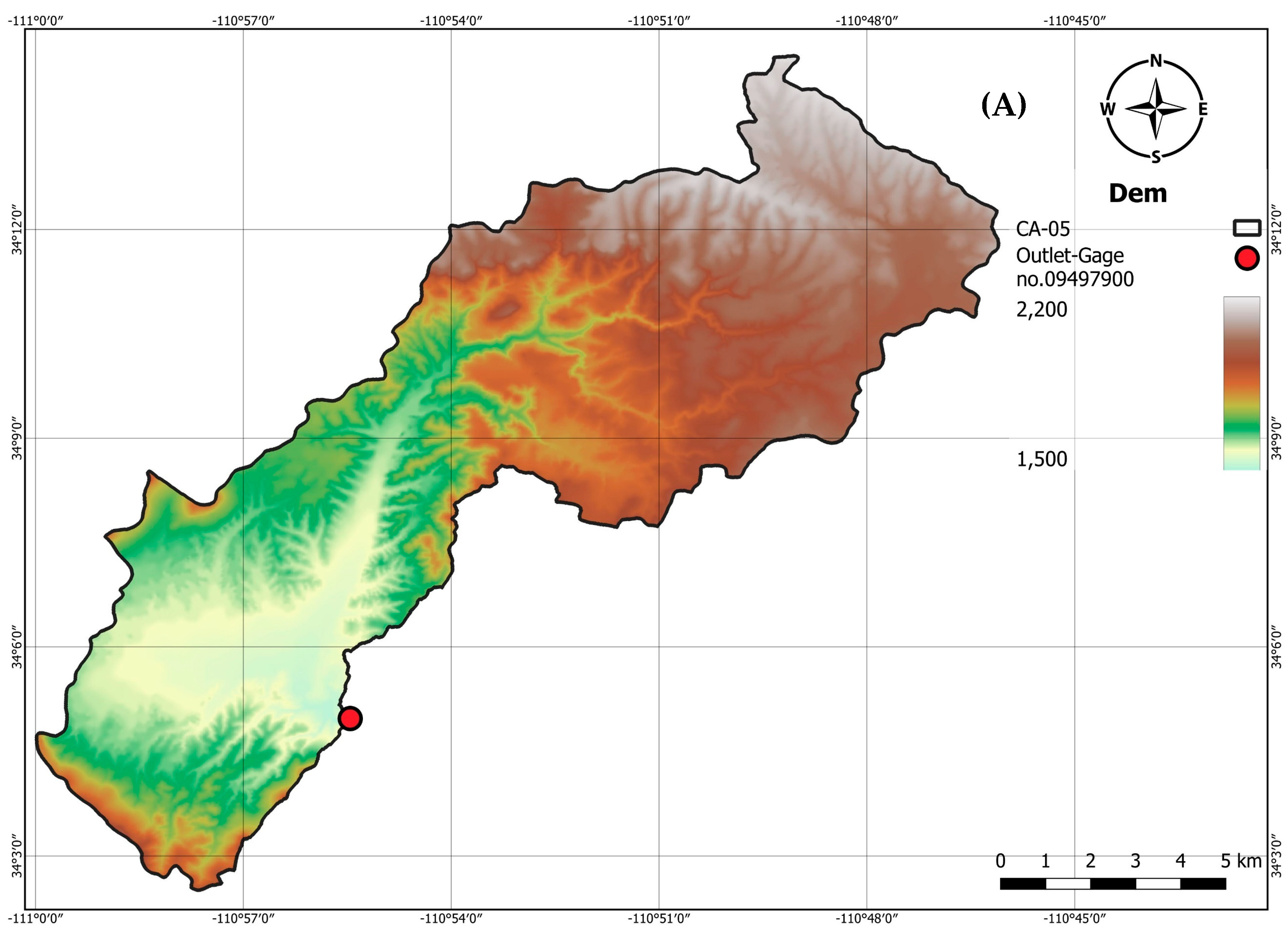
DEM and land-use maps for Catchment CA-05 (A) DEM, (B) NLCD 2019 land-use map, (C) LULC 2020-ESRI land-use map.
Figure A5.
DEM and land-use maps for Catchment CA-05 (A) DEM, (B) NLCD 2019 land-use map, (C) LULC 2020-ESRI land-use map.


Figure A6.
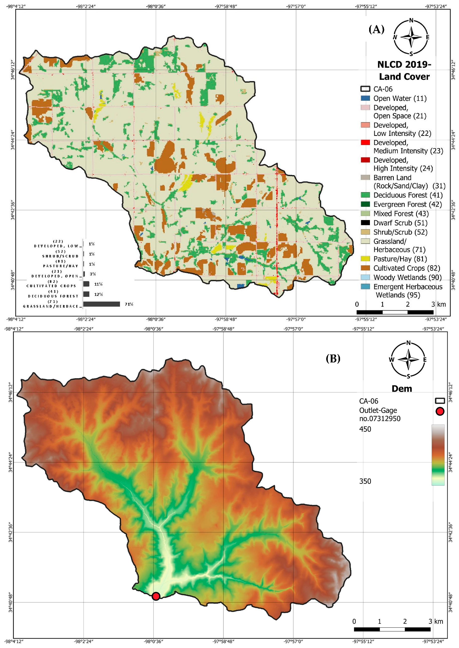
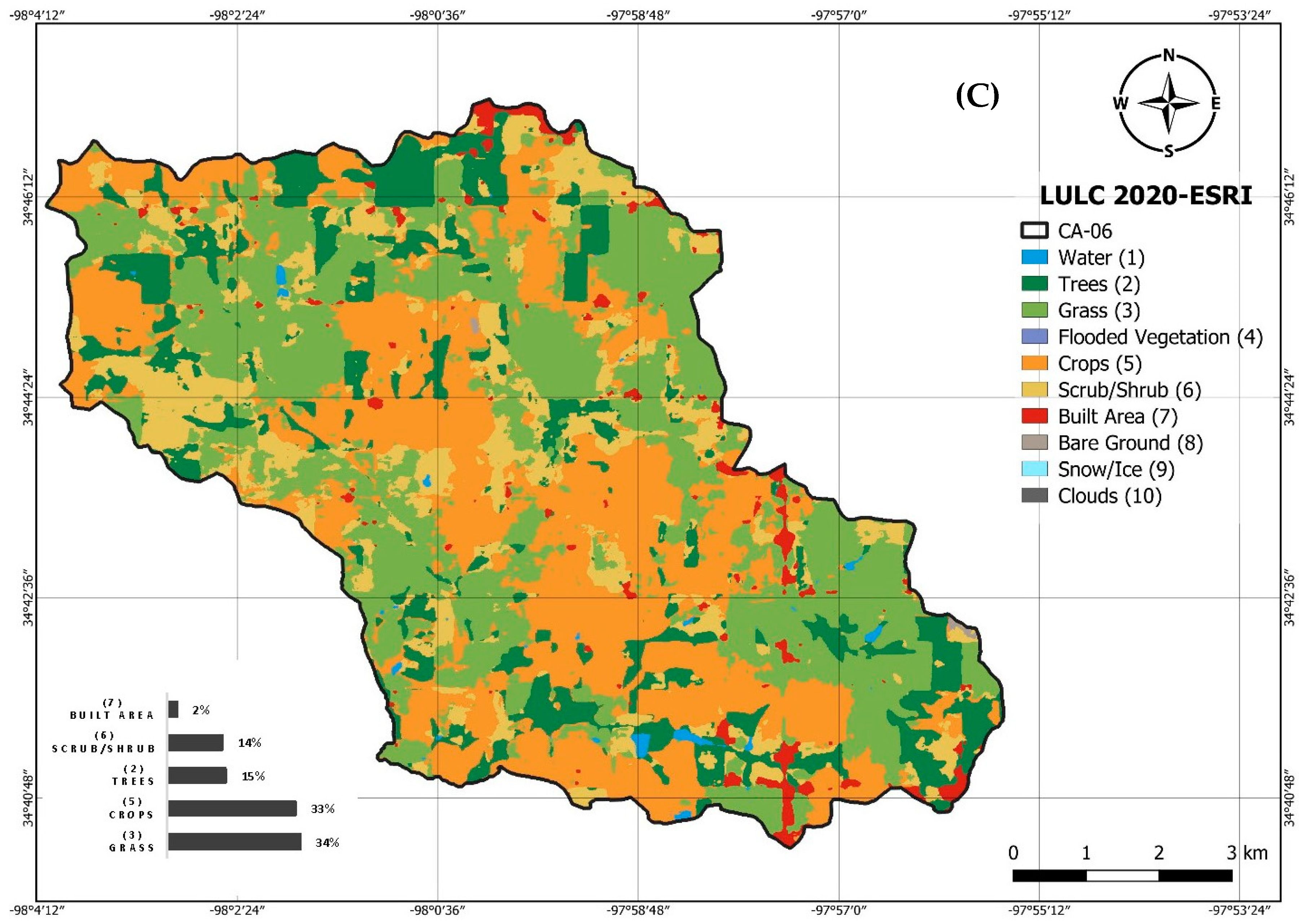
DEM and land-use maps for Catchment CA-06 (A) DEM, (B) NLCD 2019 land-use map, (C) LULC 2020-ESRI land-use map.
Figure A6.
DEM and land-use maps for Catchment CA-06 (A) DEM, (B) NLCD 2019 land-use map, (C) LULC 2020-ESRI land-use map.


Figure A7.
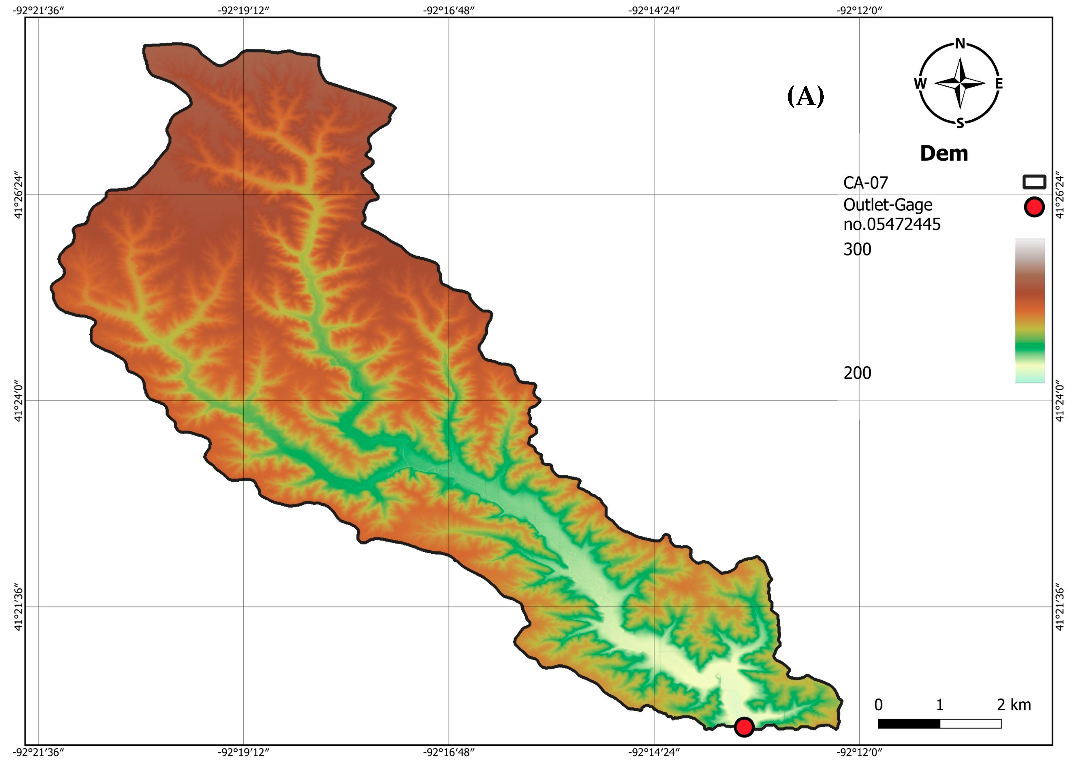
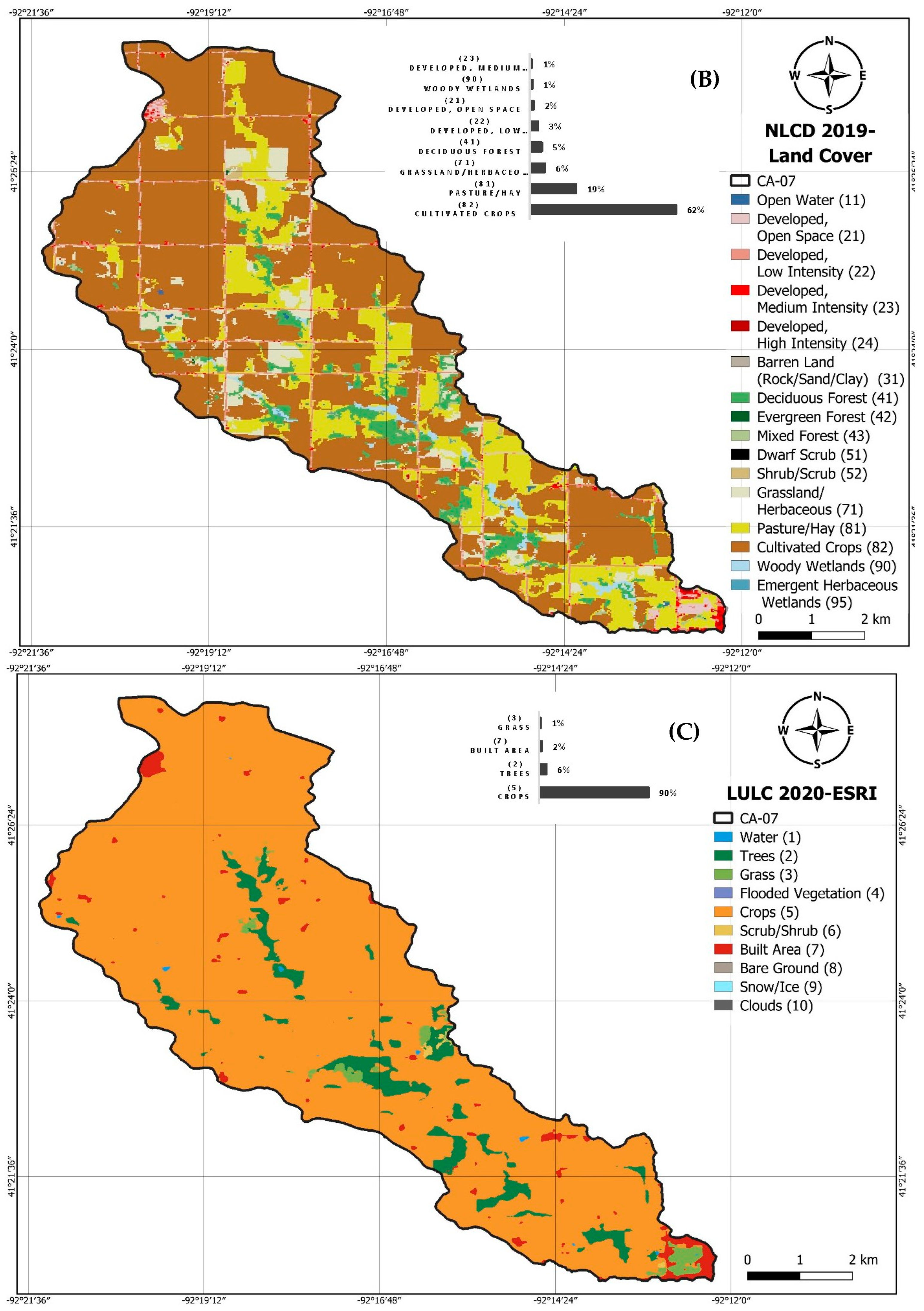
DEM and land-use maps for Catchment CA-07 (A) DEM, (B) NLCD 2019 land-use map, (C) LULC 2020-ESRI land-use map.
Figure A7.
DEM and land-use maps for Catchment CA-07 (A) DEM, (B) NLCD 2019 land-use map, (C) LULC 2020-ESRI land-use map.


Figure A8.
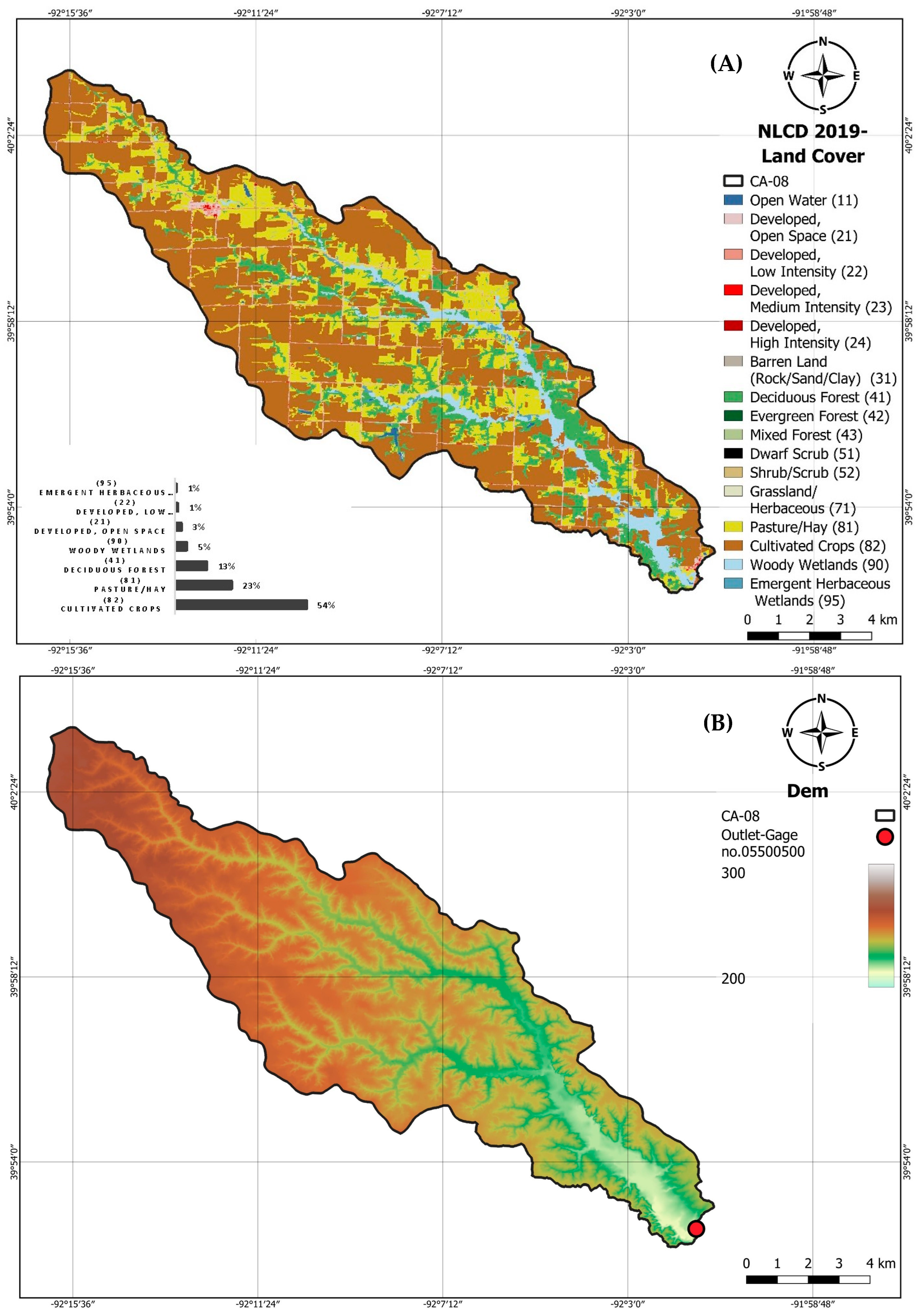
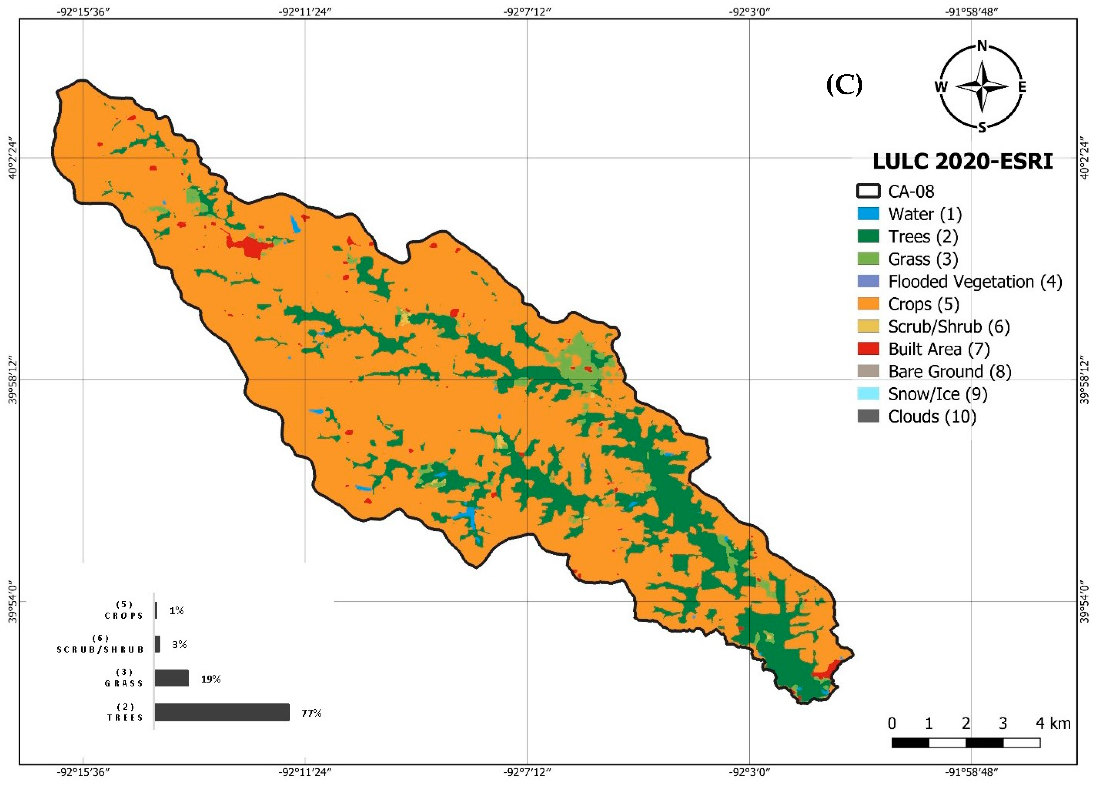
DEM and land-use maps for Catchment CA-08 (A) DEM, (B) NLCD 2019 land-use map, (C) LULC 2020-ESRI land-use map.
Figure A8.
DEM and land-use maps for Catchment CA-08 (A) DEM, (B) NLCD 2019 land-use map, (C) LULC 2020-ESRI land-use map.


Figure A9.
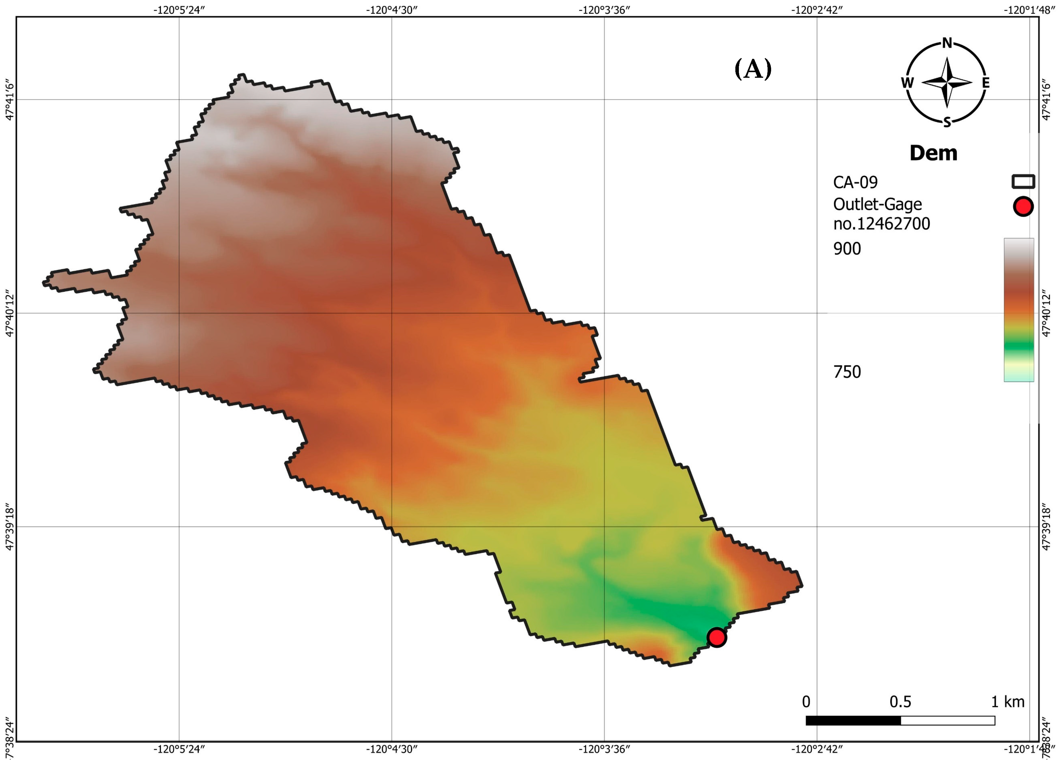
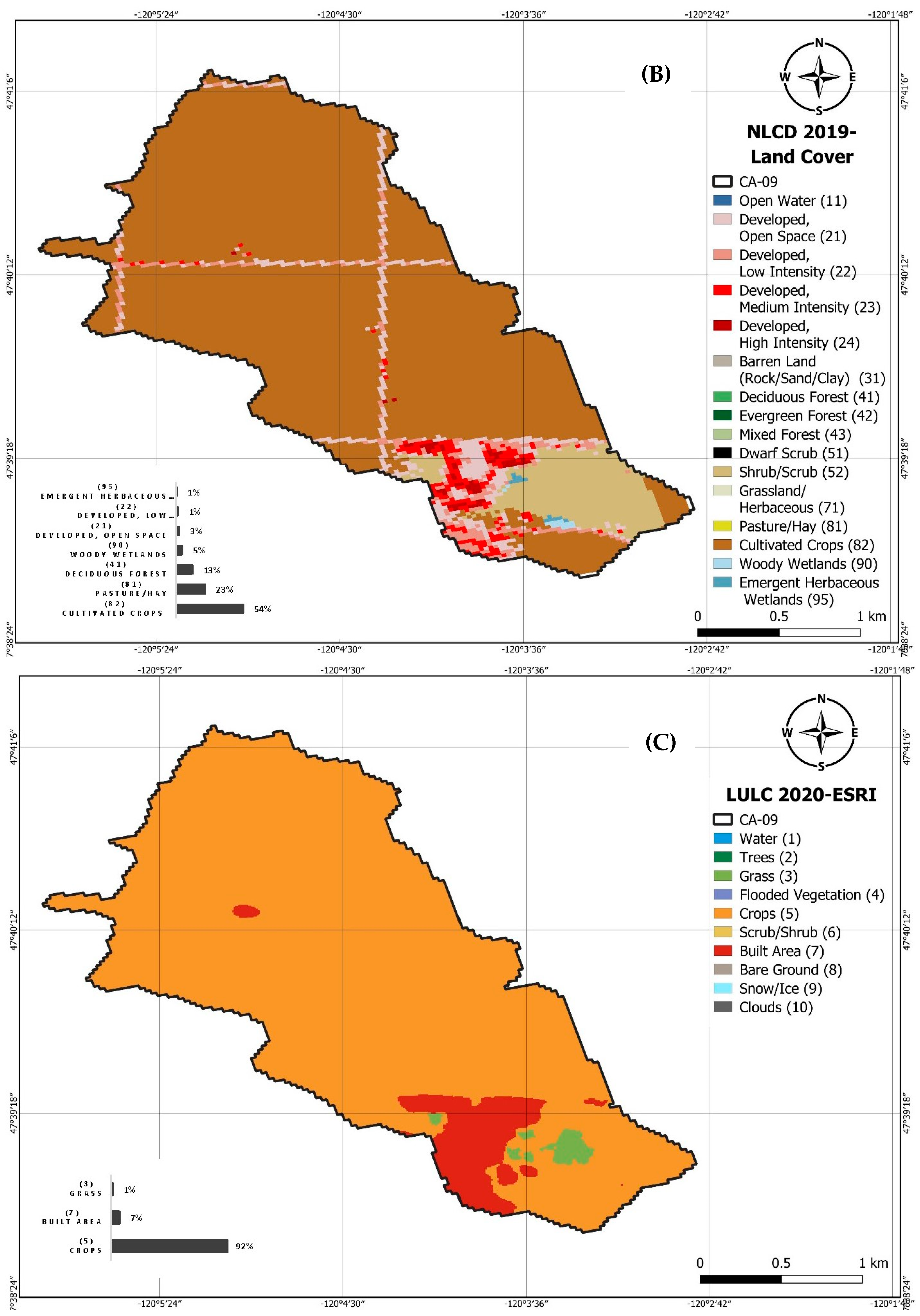
DEM and land-use maps for Catchment CA-09 (A) DEM, (B) NLCD 2019 land-use map, (C) LULC 2020-ESRI land-use map.
Figure A9.
DEM and land-use maps for Catchment CA-09 (A) DEM, (B) NLCD 2019 land-use map, (C) LULC 2020-ESRI land-use map.


Appendix B
Figure A10.
HEC-RAS 2D calibration results, maximum depth, hydrograph at outlet (A) Catchment CA-01, (B) Catchment CA-02, (C) Catchment CA-03.
Figure A10.
HEC-RAS 2D calibration results, maximum depth, hydrograph at outlet (A) Catchment CA-01, (B) Catchment CA-02, (C) Catchment CA-03.


Figure A11.
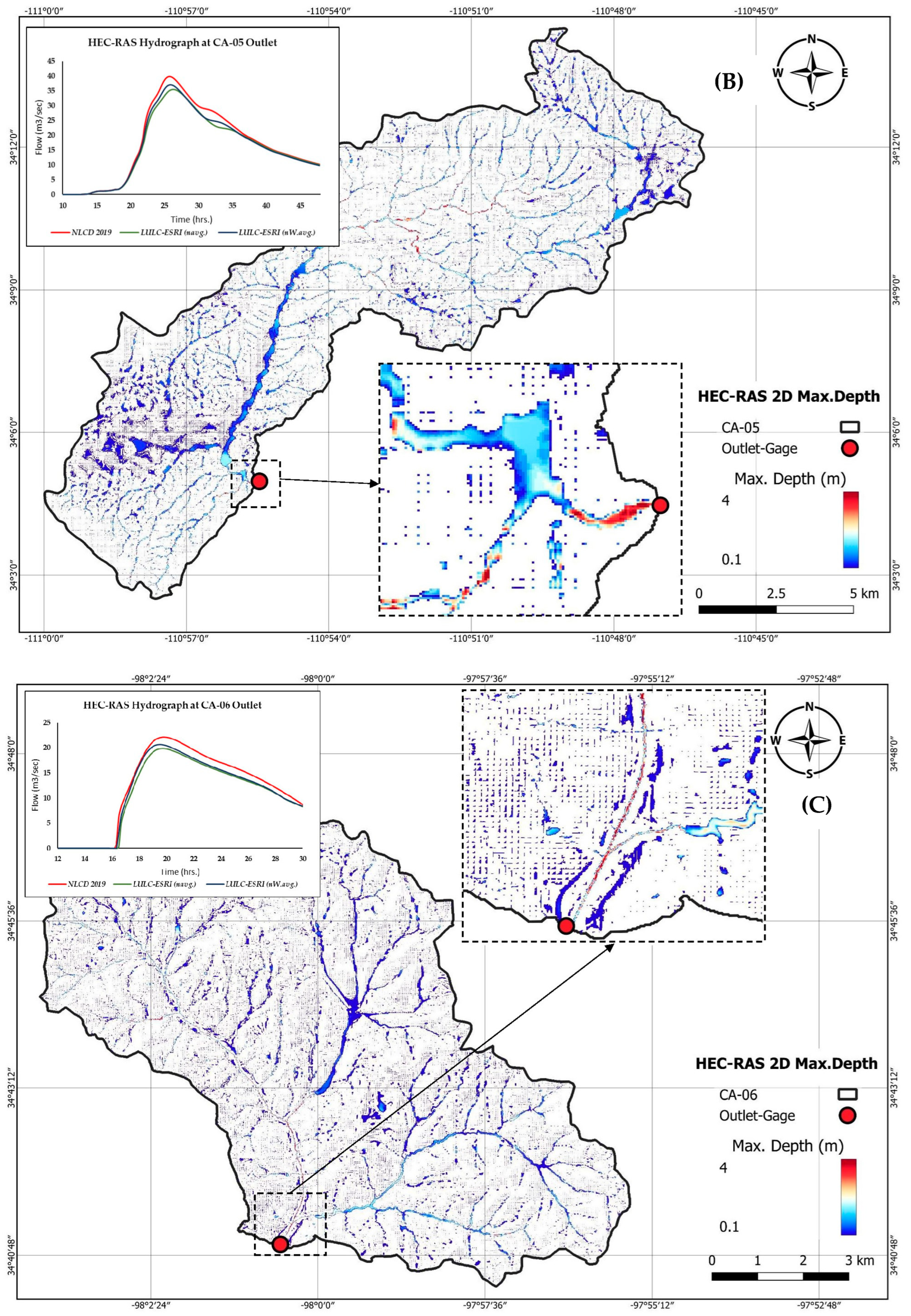
HEC-RAS 2D calibration results, maximum depth, hydrograph at outlet (A) Catchment CA-04, (B) Catchment CA-05, (C) Catchment CA-06.
Figure A11.
HEC-RAS 2D calibration results, maximum depth, hydrograph at outlet (A) Catchment CA-04, (B) Catchment CA-05, (C) Catchment CA-06.


Figure A12.
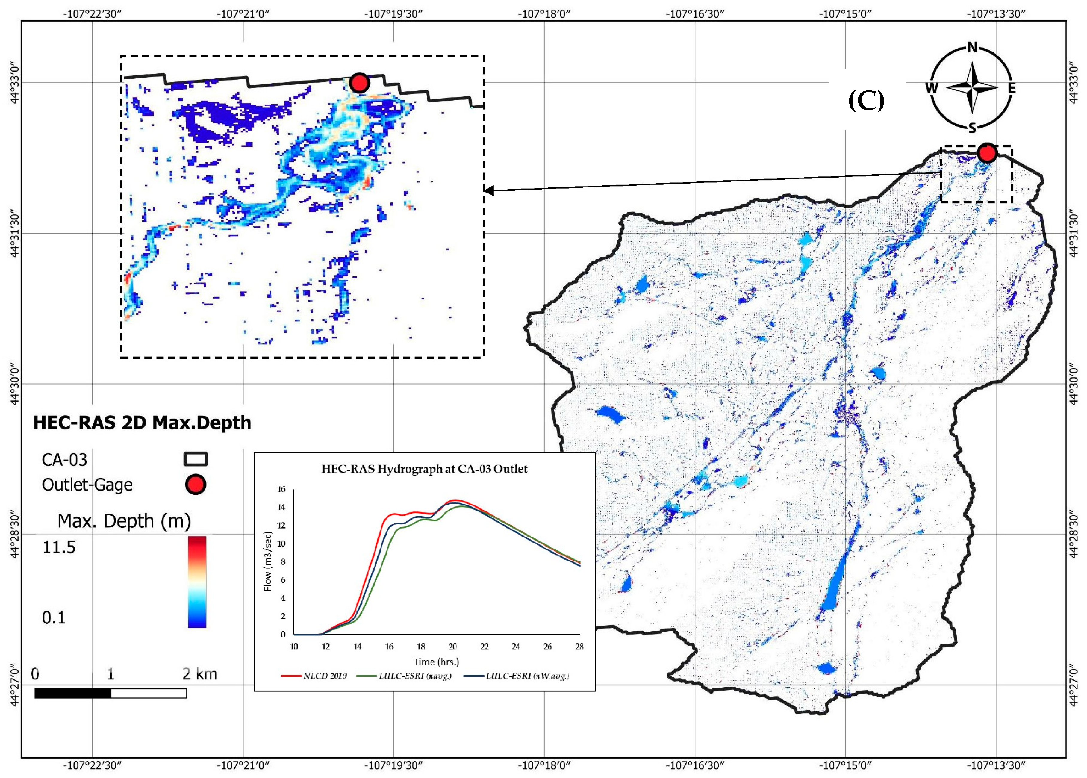
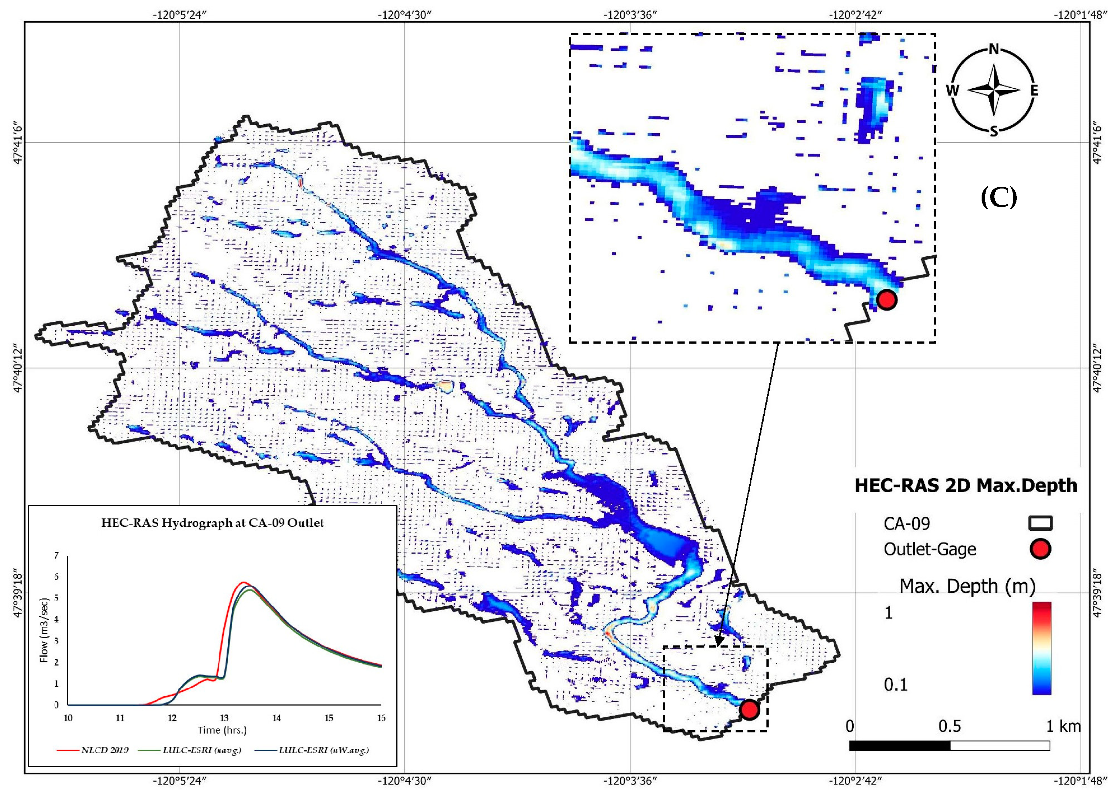
HEC-RAS 2D calibration results, maximum depth, hydrograph at outlet (A) Catchment CA-07, (B) Catchment CA-08, (C) Catchment CA-09.
Figure A12.
HEC-RAS 2D calibration results, maximum depth, hydrograph at outlet (A) Catchment CA-07, (B) Catchment CA-08, (C) Catchment CA-09.


References
- Papaioannou, G.; Vasiliades, L.; Loukas, A.; Aronica, G.T. Probabilistic flood inundation mapping at ungauged streams due to roughness coefficient uncertainty in hydraulic modelling. J. Adv. Geosci. 2017, 44, 23–34. [Google Scholar] [CrossRef] [Green Version]
- Calo, V.M.; Collier, N.; Gegre, M.; Jin, B.; Radwan, H. Gradient-based estimation of Manning’s friction coefficient from noisy data. J. Comput. Appl. Math. 2013, 238, 1–13. [Google Scholar] [CrossRef] [Green Version]
- Abbas, A.S.; Al-Aboode, A.H.; Ibrahim, H.T. Identification of Manning’s Coefficient Using HEC-RAS Model: Upstream Al-Amarah Barrage. J. Eng. 2020, 2020, 6450825. [Google Scholar] [CrossRef] [Green Version]
- Žic, E.; Vranješ, M.; Ožanić, N. Methods of roughness coefficient determination in natural riverbeds. In Proceedings of the International Symposium on Water Management and Hydraulic Engineering, Ohrid, Macedonia, 1–5 September 2009. [Google Scholar]
- HEC-RAS 2D User’s Manual; Developing a Terrain Model and Geospatial Layers; Creating Land Cover, Manning’s n Values; Table 2-1. Available online: https://www.hec.usace.army.mil/confluence/rasdocs/r2dum/latest/developing-a-terrain-model-and-geospatial-layers/creating-land-cover-mannings-n-values-and-impervious-layers (accessed on 15 May 2022).
- Ding, Y.; Jia, Y.; Wang, S.S.Y. Identification of Manning’s roughness coefficients in shallow water flows. J. Hydraul. Eng. 2004, 130, 501–510. [Google Scholar] [CrossRef] [Green Version]
- Ramesh, R.; Datta, B.; Bhallamudi, S.; Narayana, A. Optimal estimation of roughness in open-channel flows. J. Hydraul. Eng. 1997, 126, 299–303. [Google Scholar] [CrossRef]
- Ali, Z.M.D.; Abdul Karim, N.H.; Razi, M.A.M. Study on roughness coefficient at natural channel. In Proceedings of the International Conference on Environment (ICENV 2010), Penang, Malaysia, 26–29 July 2010. [Google Scholar]
- Abdul Hameed, U.H. Determination of manning roughness value for Euphrates River at Al-Falluja barrages using different theories. Iraq Acad. Sci. J. 2010, 2, 25–31. [Google Scholar]
- Parhi, P.K. HEC-RAS model for Manning’s roughness: A case study. Open J. Mod. Hydrol. 2013, 3, 97–101. [Google Scholar] [CrossRef] [Green Version]
- Shamkhi, M.S.; Attab, Z.S. Estimation of Manning’s roughness coefficient for Tigris River by using HEC-RAS model. WASIT J. Eng. Sci. 2018, 6, 90–97. [Google Scholar] [CrossRef]
- Costabile, P.; Costanzo, C.; Ferraro, D.; Barca, P. Is HEC-RAS 2D accurate enough for storm-event hazard assessment? Lessons learnt from a benchmarking study based on rain-on-grid modelling. J. Hydrol. 2021, 603, 126962. [Google Scholar] [CrossRef]
- Zeiger, S.J.; Hubbart, J.A. Measuring and modeling event-based environmental flows: An assessment of HEC-RAS 2D rain-on-grid simulations. J. Environ. Manag. 2021, 285, 112125. [Google Scholar] [CrossRef]
- Chow, V.T. Open Channel Hydraulics; McGraw-Hill Book Company, Inc.: New York, NY, USA, 1959; pp. 109–113. [Google Scholar]
- Horritt, M.S.; Bates, P.D.; Mattinson, M.J. Effects of mesh resolution and topographic representation in 2D finite volume models of shallow water fluvial flow. J. Hydrol. 2006, 329, 306–314. [Google Scholar] [CrossRef]
- Liu, Z.; Merwade, V.; Jafarzadegan, K. Investigating the role of model structure and surface roughness in generating flood inundation extents using one-and two-dimensional hydraulic models. J. Flood Risk Manag. 2019, 12, e12347. [Google Scholar] [CrossRef] [Green Version]
- Lim, N.J.C.; Brandt, S.A. Flood map boundary sensitivity due to combined effects of DEM resolution and roughness in relation to model performance. Geomat. Nat. Hazards Risk 2019, 10, 1613–1647. [Google Scholar] [CrossRef] [Green Version]
- Marks, K.; Bates, P. Integration of high-resolution topographic data with floodplain flow models. Hydrol. Processes 2000, 14, 2109–2122. [Google Scholar] [CrossRef]
- Morsy, M.M.; Lerma, N.R.; Shen, Y.; Goodall, J.L.; Huxley, C.; Sadler, J.M.; Voce, D.; O’Neil, G.L.; Maghami, I.; Zahura, F.T. Impact of Geospatial Data Enhancements for Regional-Scale 2D Hydrodynamic Flood Modeling: Case Study for the Coastal Plain of Virginia. J. Hydrol. Eng. 2021, 26, 05021002. [Google Scholar] [CrossRef]
- Merwade, V.; Olivera, F.; Arabi, M.; Edleman, S. Uncertainty in flood inundation mapping: Current issues and future directions. J. Hydrol. Eng. 2008, 13, 608–620. [Google Scholar] [CrossRef] [Green Version]
- Yalcin, E. Assessing the impact of topography and land cover data resolutions on two-dimensional HEC-RAS hydrodynamic model simulations for urban flood hazard analysis. Nat. Hazards 2020, 101, 995–1017. [Google Scholar] [CrossRef]
- Buchhorn, M.; Lesiv, M.; Tsendbazar, N.E.; Herold, M.; Bertels, L.; Smets, B. Copernicus global land cover layers—Collection 2. Remote Sens. 2020, 12, 1044. [Google Scholar] [CrossRef] [Green Version]
- Pande, C.B.; Moharir, K.N.; Khadri, S.F.R.; Patil, S. Study of land use classification in an arid region using multispectral satellite images. Appl. Water Sci. 2018, 8, 123. [Google Scholar] [CrossRef] [Green Version]
- Cole, L.J.; Kleijn, D.; Dicks, L.V.; Stout, J.C.; Potts, S.G.; Albrecht, M.; Balzan, M.V.; Bartomeus, I.; Bebeli, P.J.; Bevk, D.; et al. A critical analysis of the potential for E.U. Common Agricultural Policy measures to support wild pollinators on farmland. J. Appl. Ecol. 2020, 57, 681–694. [Google Scholar] [CrossRef]
- Zhu, Z.; Wulder, M.A.; Roy, D.P.; Woodcock, C.E.; Hansen, M.C.; Radeloff, V.C.; Healey, S.P.; Schaaf, C.; Hostert, P.; Strobl, P.; et al. Benefits of the free and open Landsat data policy. Remote Sens. Environ. 2019, 224, 382–385. [Google Scholar] [CrossRef]
- Gorelick, N.; Hancher, M.; Dixon, M.; Ilyushchenko, S.; Thau, D.; Moore, R. Google Earth Engine: Planetary-scale geospatial analysis for everyone. Remote Sens. Environ. 2017, 202, 18–27. [Google Scholar] [CrossRef]
- Pande, C.B. Land Use/Land Cover and Change Detection mapping in Rahuri watershed area (MS), India using the Google Earth Engine and Machine Learning Approach. Geocarto Int. 2022, 1–15. [Google Scholar] [CrossRef]
- Pande, C.B.; Moharir, K.N.; Singh, S.K.; Varade, A.M.; Elbeltagi, A.; Khadri, S.F.R.; Choudhari, P. Estimation of crop and forest biomass resources in a semi-arid region using satellite data and GIS. J. Saudi Soc. Agric. Sci. 2021, 20, 302–311. [Google Scholar] [CrossRef]
- Pande, C.B.; Moharir, K.N.; Khadri, S.F.R. Assessment of land-use and land-cover changes in Pangari watershed area (MS), India, based on the remote sensing and GIS techniques. Appl. Water Sci. 2021, 11, 1–12. [Google Scholar] [CrossRef]
- Alam, A.; Bhat, M.S.; Maheen, M. Using Landsat satellite data for assessing the land use and land cover change in Kashmir valley. GeoJournal 2020, 85, 1529–1543. [Google Scholar] [CrossRef] [Green Version]
- Dewitz, J. National Land Cover Database (NLCD) 2019 Products [Dataset]; US Geological Survey: Sioux Falls, SD, USA, 2021. Available online: https://data.usgs.gov/datacatalog/data/USGS:60cb3da7d34e86b938a30cb9 (accessed on 9 March 2022).
- Wickham, J.; Stehman, S.V.; Sorenson, D.G.; Gass, L.; Dewitz, J.A. Thematic accuracy assessment of the NLCD 2016 land cover for the conterminous United States. Remote Sens. Environ. 2021, 257, 112357. [Google Scholar] [CrossRef]
- Karra, K.; Kontgis, C.; Statman-Weil, Z.; Mazzariello, J.C.; Mathis, M.; Brumby, S.P. Global land use/land cover with Sentinel 2 and deep learning. In Proceedings of the 2021 IEEE International Geoscience and Remote Sensing Symposium IGARSS, Brussels, Belgium, 11–16 July 2021; IEEE: Piscataway, NJ, USA, 2021; pp. 4704–4707. [Google Scholar]
- Huan, V.D. Accuracy assessment of land use land cover LULC 2020 (ESRI) data in Con Dao Island, Ba Ria–Vung Tau province, Vietnam. In IOP Conference Series: Earth and Environmental Science; IOP Publishing: Bristol, UK, 2022; Volume 1028, p. 012010. [Google Scholar]
- Venter, Z.S.; Barton, D.N.; Chakraborty, T.; Simensen, T.; Singh, G. Global 10 m Land Use Land Cover Datasets: A Comparison of Dynamic World, World Cover and Esri Land Cover. Remote Sens. 2022, 14, 4101. [Google Scholar] [CrossRef]
- Kalyanapu, A.J.; Burian, S.J.; McPherson, T.N. Effect of land use-based surface roughness on hydrologic model output. J. Spat. Hydrol. 2009, 9, 51–71. [Google Scholar]
- Ries, K.G., III; Newson, J.K.; Smith, M.J.; Guthrie, J.D.; Steeves, P.A.; Haluska, T.L.; Kolb, K.R.; Thompson, R.F.; Santoro, R.D.; Vraga, H.W. StreamStats, version 4; US Geological Survey: Reston, VA, USA, 2017; Volume 3046, p. 4. [Google Scholar] [CrossRef] [Green Version]
- Bonnin, G.M.; Martin, D.; Lin, B.; Parzybok, T.; Yekta, M.; Riley, D. Precipitation-Frequency Atlas of the United States: NOAA Atlas 14, version 4; NOAA, National Weather Service: Silver Spring, MD, USA, 2006; Volume 1. [Google Scholar]
- Brunner, G.W. HEC-RAS River Analysis System 2D Modeling User’s Manual; U.S. Army Corps of Engineers—Hydrologic Engineering Center: Washington, DC, USA, 2016; pp. 1–171. [Google Scholar]
- Quirogaa, V.M.; Kurea, S.; Udoa, K.; Manoa, A. Application of 2D numerical simulation for the analysis of the February 2014 Bolivian Amazonia flood: Application of the new HEC-RAS version 5. Ribagua 2016, 3, 25–33. [Google Scholar] [CrossRef] [Green Version]
- David, A.; Schmalz, B. A systematic analysis of the interaction between rain-on-grid-simulations and spatial resolution in 2D hydrodynamic modeling. Water 2021, 13, 2346. [Google Scholar] [CrossRef]
- Soil Conservation Service (SCS, U). National Engineering Handbook, Section 4: Hydrology; U.S. Soil Conservation Service, USDA: Washington, DC, USA, 1985. Available online: https://directives.sc.egov.usda.gov/OpenNonWebContent.aspx?content=18393.wba (accessed on 10 March 2022).
- Costabile, P.; Costanzo, C.; Ferraro, D.; Macchione, F.; Petaccia, G. Performances of the new HEC-RAS version 5 for 2-D hydrodynamic-based rainfall-runoff simulations at basin scale: Comparison with a state-of-the art model. Water 2020, 12, 2326. [Google Scholar] [CrossRef]
- Brown, C.F.; Brumby, S.P.; Guzder-Williams, B.; Birch, T.; Hyde, S.B.; Mazzariello, J.; Czerwinski, W.; Pasquarella, V.J.; Haertel, R.; Ilyushchenko, S.; et al. Dynamic World, Near real-time global 10 m land use land cover mapping. Sci. Data 2022, 9, 251. [Google Scholar] [CrossRef]
- U.S. Geological Survey. USGS 3D Elevation Program Digital Elevation Model. 2019. Available online: https://elevation.nationalmap.gov/arcgis/rest/services/3DEPElevation/ImageServer (accessed on 20 March 2022).
- Hariri, S.; Weill, S.; Gustedt, J.; Charpentier, I. A balanced watershed decomposition method for rain-on-grid simulations in HEC-RAS. J. Hydroinform. 2022, 24, 315–332. [Google Scholar] [CrossRef]
- Bessar, M.A.; Matte, P.; Anctil, F. Uncertainty analysis of a 1d river hydraulic model with adaptive calibration. Water 2020, 12, 561. [Google Scholar] [CrossRef]
- Cronshey, R. Urban Hydrology for Small Watersheds; U.S. Dept. of Agriculture, Soil Conservation Service, Engineering Division: Washington, DC, USA, 1986.
Figure 1.
NLCD 2019 Classifications [31].
Figure 1.
NLCD 2019 Classifications [31].

Figure 2.
LULC 2020-ESRI classifications for conterminous United States only [33].
Figure 2.
LULC 2020-ESRI classifications for conterminous United States only [33].

Figure 3.
Research methodology for part 1: data preparation, accuracy assessment, and roughness analysis.
Figure 3.
Research methodology for part 1: data preparation, accuracy assessment, and roughness analysis.

Figure 4.
Research methodology for part 2: calibrating and validating the developed roughness maps using flood modeling.
Figure 4.
Research methodology for part 2: calibrating and validating the developed roughness maps using flood modeling.

Figure 5.
Frequency analysis for the extracted samples from the NLCD 2019 dataset.

Figure 6.
Frequency analysis for the extracted samples from the LULC 2020-ESRI dataset.

Figure 7.
Frequency analysis for the biased classes from the LULC 2020-ESRI map. (A) Tree, (B) Built area, (C) Grass.
Figure 7.
Frequency analysis for the biased classes from the LULC 2020-ESRI map. (A) Tree, (B) Built area, (C) Grass.


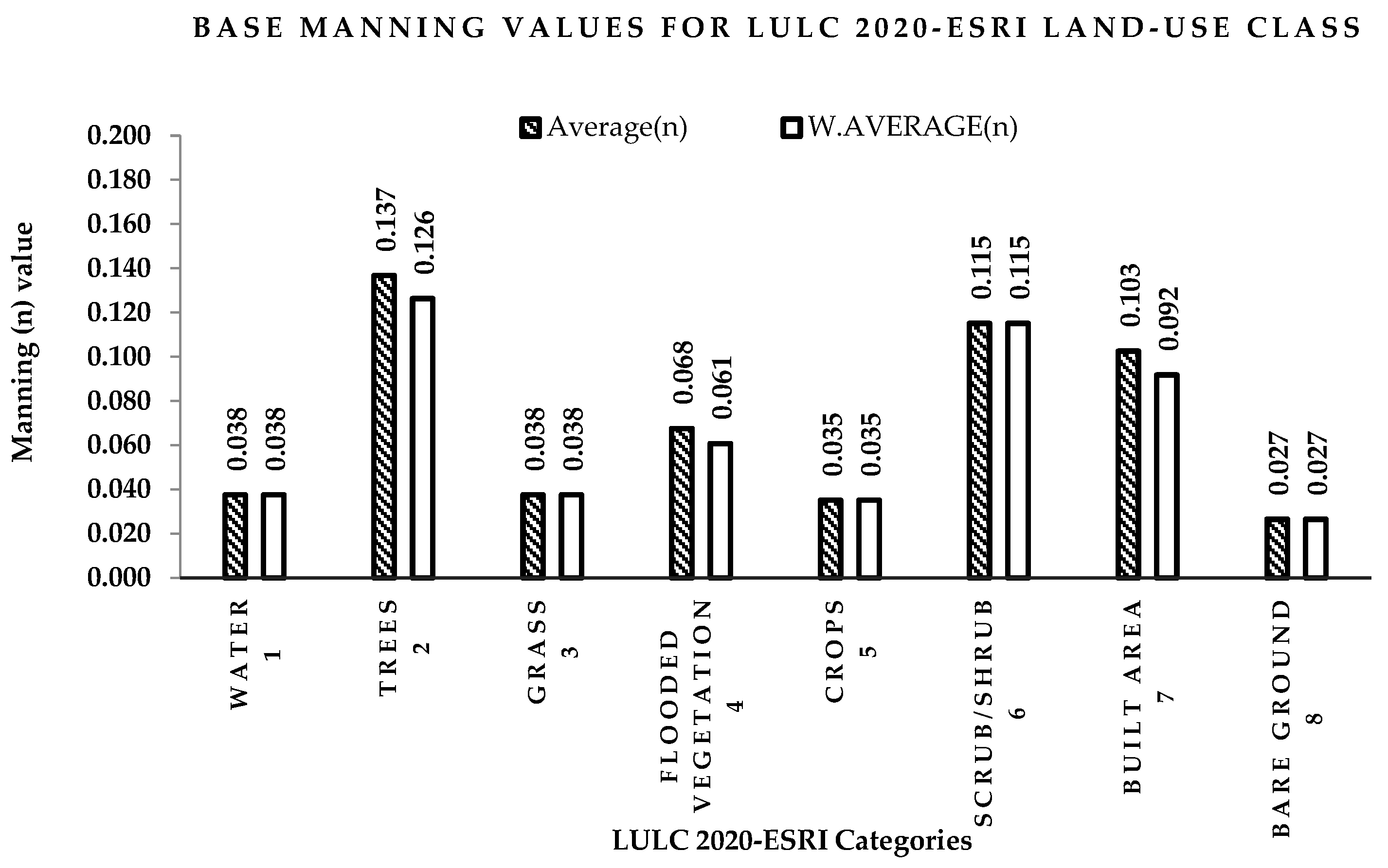
Figure 8.
LULC 2020-ESRI base Manning’s roughness values using both average and weighted average methods.
Figure 8.
LULC 2020-ESRI base Manning’s roughness values using both average and weighted average methods.

Figure 9.
The selected nine catchments’ locations on a satellite-based image.

Figure 10.
DEM and land-use maps for Catchment CA-01 (A) DEM, (B) NLCD 2019 land-use map, (C) LULC 2020-ESRI land-use map.
Figure 10.
DEM and land-use maps for Catchment CA-01 (A) DEM, (B) NLCD 2019 land-use map, (C) LULC 2020-ESRI land-use map.


Figure 11.
HEC-RAS calibration outputs: flow hydrographs at catchment outlet and maximum depths over the catchment area for CA-01.
Figure 11.
HEC-RAS calibration outputs: flow hydrographs at catchment outlet and maximum depths over the catchment area for CA-01.

Figure 12.
Peak-flow error using LULC 2020-ESRI along with (navg) and (nw.avg) values compared to the base calibrated results.
Figure 12.
Peak-flow error using LULC 2020-ESRI along with (navg) and (nw.avg) values compared to the base calibrated results.

Figure 13.
Peak-flow error using LULC 2020-ESRI along with (navg) and (nw.avg) values compared to the base validation results.
Figure 13.
Peak-flow error using LULC 2020-ESRI along with (navg) and (nw.avg) values compared to the base validation results.

Figure 14.
Time to peak flow in hours using LULC 2020-ESRI with (navg) and (nw.avg), compared to base map calibration results.
Figure 14.
Time to peak flow in hours using LULC 2020-ESRI with (navg) and (nw.avg), compared to base map calibration results.

Figure 15.
Time to peak flow in hours using LULC 2020-ESRI with (navg) and (nw.avg), compared to base map validation results.
Figure 15.
Time to peak flow in hours using LULC 2020-ESRI with (navg) and (nw.avg), compared to base map validation results.


Table 1.
NLCD 2019 Classifications and detailed topology descriptions [31].
Table 1.
NLCD 2019 Classifications and detailed topology descriptions [31].
| NLCD Value | Description | Detailed Description |
|---|---|---|
| 95 | Emergent Herbaceous Wetlands | Areas where perennial herbaceous vegetation accounts for more than 80% of vegetative cover and the soil or substrate is covered with water or periodically saturated with water. |
| 90 | Woody Wetlands | Areas where forest or shrub land vegetation accounts for greater than 20% of vegetative cover and the soil or substrate is periodically saturated with or covered with water. |
| 82 | Cultivated Crops | Areas used for the production of annual crops, such as corn, soybeans, vegetables, tobacco, and cotton, and also perennial woody crops such as orchards and vineyards. Crop vegetation accounts for greater than 20% of total vegetation. This class also includes all land being actively tilled. |
| 81 | Pasture/Hay | Areas of grasses, legumes, grass-legume mixtures planted for livestock grazing or the production of seed or hay crops, typically on a perennial cycle. Pasture/hay vegetation accounts for greater than 20% of total vegetation. |
| 71 | Grassland/Herbaceous | Areas dominated by gramanoid or herbaceous vegetation, generally greater than 80% of total vegetation. These areas are not subject to intensive management such as tilling, but can be utilized for grazing. |
| 52 | Shrub/Scrub | Areas dominated by shrubs; less than 5 m tall with shrub canopy typically greater than 20% of total vegetation. This class includes true shrubs, young trees in an early successional stage or trees stunted from environmental conditions. |
| 51 | Dwarf Scrub | Alaska only areas dominated by shrubs less than 20 cm tall with shrub canopy typically greater than 20% of total vegetation. his type is often co-associated with grasses, sedges, herbs, and non-vascular vegetation. |
| 43 | Mixed Forest | Areas dominated by trees generally greater than 5 m tall, and greater than 20% of total vegetation cover. Neither deciduous nor evergreen species are greater than 75% of total tree cover. |
| 42 | Evergreen Forest | Areas dominated by trees generally greater than 5 m tall, and greater than 20% of total vegetation cover. More than 75% of the tree species maintain their leaves all year. Canopy is never without green foliage. |
| 41 | Deciduous Forest | Areas dominated by trees generally greater than 5 m tall, and greater than 20% of total vegetation cover. More than 75% of the tree species shed foliage simultaneously in response to seasonal change. |
| 31 | Barren Land (Rock/Sand/Clay) | Areas of bedrock, desert pavement, scarps, talus, slides, volcanic material, glacial debris, sand dunes, strip mines, gravel pits and other accumulations of earthen material. Generally, vegetation accounts for less than 15% of total cover. |
| 24 | Developed, High Intensity | Highly developed areas where people reside or work in high numbers. Examples include apartment complexes, row houses and commercial/industrial. Impervious surfaces account for 80% to 100% of the total cover. |
| 23 | Developed, Medium Intensity | areas with a mixture of constructed materials and vegetation. Impervious surfaces account for 50% to 79% of the total cover. These areas most commonly include single-family housing units. |
| 22 | Developed, Low Intensity | areas with a mixture of constructed materials and vegetation. Impervious surfaces account for 20% to 49% percent of total cover. These areas most commonly include single-family housing units. |
| 21 | Developed, Open Space | areas with a mixture of some constructed materials, but mostly vegetation in the form of lawn grasses. Impervious surfaces account for less than 20% of total cover. These areas most commonly include large-lot single-family housing units, parks, golf courses, and vegetation planted in developed settings for recreation, erosion control, or aesthetic purposes. |
| 11 | Open Water | Areas of open water, generally with less than 25% cover of vegetation or soil. |
Table 2.
LULC 2020-ESRI classifications and detailed topology descriptions [33].
Table 2.
LULC 2020-ESRI classifications and detailed topology descriptions [33].
| LULC Value | Description | Detailed Description |
|---|---|---|
| 1 | Water | Examples of areas having year-round water include rivers, ponds, lakes, oceans, and flooded salt plains. These areas may not include areas with intermittent or ephemeral water, little to no sparse vegetation, no rock outcrops, and no built-up features such as docks. |
| 2 | Trees | Any notable grouping of tall (15 m or higher) dense vegetation, usually with a closed or dense canopy; examples include wooded vegetation, dense tall vegetation groups in savannas, plantations, swamps, or mangroves (dense/tall vegetation with ephemeral water or canopy too thick to detect water underneath). |
| 3 | Grass | Examples include natural meadows and fields with little to no tree cover, open savanna with few to no trees, parks/golf courses/lawns, and pastures. Open areas covered in homogenous grasses with little to no taller vegetation; wild cereals and grasses without obvious human plotting (i.e., not a plotted field). |
| 4 | Flooded vegetation | Any area with vegetation of any kind that is clearly interspersed with water for the majority of the year; a seasonal floodplain that contains a mixture of grass, shrubs, trees, and bare ground. Examples include flooded mangroves, emergent vegetation, rice paddies, and other heavily irrigated and inundated agricultural areas. |
| 5 | Crops | Cereals, grasses, and crops not at tree height that have been planted or plotted by humans include corn, wheat, soy, and fallow areas of structured land. |
| 6 | Scrub/shrub | A mixture of small groupings of plants or lone plants scattered across a landscape with exposed rock or dirt; thick woodlands with visible gaps that are plainly not taller than trees; examples include savannas with very scant grasses, trees, or other vegetation, and areas with a moderate to sparse cover of bushes, shrubs, and tufts of grass. |
| 7 | Built Area | Large homogenous impervious surfaces, such as parking garages, office buildings, and residential dwellings, are all man-made structures. Examples include houses, dense villages, towns, and cities, paved highways, and asphalt. |
| 8 | Bare ground | Examples include exposed rock or soil, deserts and sand dunes, arid salt flats/pans, dried lake beds, mines, and areas of rock or soil with very little to no vegetation during the entire year. |
| 9 | Snow/Ice | Large, uniform patches of always-present snow or ice, usually found exclusively in mountainous regions or the northernmost latitudes; examples include glaciers, the permanent snowpack, and snow fields. |
| 10 | Clouds | Continual cloud cover prevents information on land coverings. |
Table 3.
NLCD-Manning’s n Values Reference Table based on Chow-1959 [5].
Table 3.
NLCD-Manning’s n Values Reference Table based on Chow-1959 [5].
| NLCD Topology Value | Description | Manning’s Roughness (n) Value Range | Manning’s Roughness (n) Average |
|---|---|---|---|
| 95 | Emergent Herbaceous Wetlands | 0.05–0.085 | 0.068 |
| 90 | Woody Wetlands | 0.045–0.15 | 0.098 |
| 82 | Cultivated Crops | 0.020–0.05 | 0.035 |
| 81 | Pasture/Hay | 0.025–0.05 | 0.038 |
| 72 | Sedge/Herbaceous | 0.025–0.05 | 0.038 |
| 71 | Grassland/Herbaceous | 0.025–0.05 | 0.038 |
| 52 | Shrub/Scrub | 0.07–0.16 | 0.115 |
| 51 | Dwarf Scrub | 0.025–0.05 | 0.038 |
| 43 | Mixed Forest | 0.08–0.20 | 0.140 |
| 42 | Evergreen Forest | 0.08–0.16 | 0.120 |
| 41 | Deciduous Forest | 0.10–0.20 | 0.150 |
| 31 | Barren Land (Rock/Sand/Clay) | 0.023–0.030 | 0.027 |
| 24 | Developed, High Intensity | 0.12–0.20 | 0.160 |
| 23 | Developed, Medium Intensity | 0.08–0.16 | 0.120 |
| 22 | Developed, Low Intensity | 0.06–0.12 | 0.090 |
| 21 | Developed, Open Space | 0.03–0.05 | 0.040 |
| 11 | Open Water | 0.025–0.05 | 0.038 |
Table 4.
Accuracy Assessment-Confusion Matrix.
| NLCD 2019 (Reference Layer) | LULC 2020-ESRI (User’s Layer) | |||||||
|---|---|---|---|---|---|---|---|---|
| Water (1) | Trees (2) | Grass (3) | Flooded Vegetation (4) | Crops (5) | Scrub/Shrub (6) | Built Area (7) | Bare Ground (8) | |
| Open Water (11) | 17,175 | 127 | 50 | 107 | 117 | 246 | 48 | 115 |
| Developed, Open Space (21) | 25 | 2712 | 882 | 21 | 1942 | 1464 | 4624 | 49 |
| Developed, Low Intensity (22) | 25 | 535 | 262 | 1 | 1101 | 411 | 5980 | 25 |
| Developed, Medium Intensity (23) | 21 | 105 | 41 | 3 | 329 | 170 | 5528 | 43 |
| Developed, High Intensity (24) | 9 | 7 | 1 | 0 | 43 | 27 | 2941 | 13 |
| Barren Land (31) | 96 | 50 | 25 | 9 | 56 | 2052 | 147 | 3188 |
| Deciduous Forest (41) | 127 | 35,081 | 723 | 62 | 721 | 2679 | 605 | 1 |
| Evergreen Forest (42) | 56 | 48,243 | 274 | 19 | 282 | 17,734 | 558 | 64 |
| Mixed Forest (43) | 45 | 11,332 | 205 | 11 | 117 | 542 | 364 | 0 |
| Shrub/Scrub (52) | 78 | 7279 | 1340 | 15 | 3353 | 119,366 | 940 | 1156 |
| Grassland/Herbaceous (71) | 186 | 2080 | 5875 | 123 | 7882 | 59,054 | 932 | 617 |
| Pasture/Hay (81) | 88 | 3246 | 10,822 | 109 | 8706 | 3179 | 1102 | 21 |
| Cultivated Crops (82) | 78 | 1120 | 1828 | 135 | 108,515 | 2863 | 674 | 196 |
| Woody Wetlands (90) | 176 | 13,409 | 404 | 127 | 427 | 1487 | 117 | 9 |
| Emergent Herbaceous Wetlands (95) | 194 | 678 | 797 | 888 | 1097 | 2342 | 99 | 52 |
| TOTAL | 18,379 | 126,004 | 23,529 | 1630 | 134,688 | 213,616 | 24,659 | 5549 |
| TRUE | 17175 | 108,065 | 16,697 | 888 | 108,515 | 119,366 | 19,073 | 3188 |
| Class Accuracy | 93% | 86% | 71% | 54% | 81% | 56% | 77% | 57% |
| Overall Accuracy | 72% | |||||||
Table 5.
LULC 2020-ESRI proposed roughness values using average and weighted average methods.
| LULC 2020-ESRI Value | 1 | 2 | 3 | 4 | 5 | 6 | 7 | 8 |
|---|---|---|---|---|---|---|---|---|
| Class Description | Water | Trees | Grass | Flooded Vegetation | Crops | Scrub/Shrub | Built Area | Bare Ground |
| NLCD Corresponding class Values | 11 | 42- 41- 43- 90 | 81- 71 | 95 | 82 | 52 | 22- 21- 23- 24 | 31 |
| Average Method-Suggested Roughness Values | ||||||||
| Minimum (n) | 0.025 | 0.087 | 0.025 | 0.05 | 0.02 | 0.07 | 0.073 | 0.023 |
| Maximum (n) | 0.050 | 0.160 | 0.050 | 0.085 | 0.050 | 0.160 | 0.132 | 0.030 |
| Average (n) | 0.038 | 0.137 | 0.038 | 0.068 | 0.035 | 0.115 | 0.103 | 0.027 |
| Weighted Average Method-Suggested Roughness Values | ||||||||
| Minimum (n) | 0.025 | 0.079 | 0.025 | 0.050 | 0.020 | 0.070 | 0.064 | 0.023 |
| Maximum (n) | 0.050 | 0.174 | 0.050 | 0.085 | 0.050 | 0.160 | 0.119 | 0.030 |
| Average (n) | 0.038 | 0.126 | 0.038 | 0.061 | 0.035 | 0.115 | 0.092 | 0.027 |
Table 6.
Locations and areas for the selected catchments.
| Catchment | Outlet-Location (UTM-WGS 84) | Catchment Area (km2) | Gage Number | ||
|---|---|---|---|---|---|
| State | Latitude | Longitude | |||
| CA-01 | Oregon | 43.25261790 | −123.0261716 | 459.47 | 14318000 |
| CA-02 | Idaho | 42.03277500 | −115.3686083 | 217.29 | 13162500 |
| CA-03 | Wyoming | 44.53830075 | −107.2264592 | 50.78 | 06300500 |
| CA-04 | Colorado | 39.33415000 | −106.5753000 | 18.73 | 09078200 |
| CA-05 | Arizona | 34.08282162 | −110.9242900 | 161.02 | 09497900 |
| CA-06 | Oklahoma | 34.68258000 | −98.00893000 | 90.21 | 07312950 |
| CA-07 | Iowa | 41.33667771 | −92.22240371 | 67.95 | 05472445 |
| CA-08 | St.Louis | 39.87476000 | −92.02406000 | 149.27 | 05500500 |
| CA-09 | Washington | 47.64707639 | −120.0539556 | 7.82 | 12462700 |
Table 7.
Rainfall, peak flow, and calibrated curve number (CN) data for the selected catchments [37,38].
| Catchment | Catchment Area (km2) | Selected (SCS-CN) | 2-Year Return Period | 100-Year Return Period | ||
|---|---|---|---|---|---|---|
| Precipitation P (mm) | Peak Flow Q (m3/s) | Precipitation P (mm) | Peak Flow Q (m3/s) | |||
| CA-01 | 459.47 | 77 | 66.5 | 268.2 | N/A | N/A |
| CA-02 | 217.29 | 72 | 33.0 | 12.6 | N/A | N/A |
| CA-03 | 50.78 | 74 | 63.5 | 15.0 | N/A | N/A |
| CA-04 | 18.73 | 80 | 40.6 | 3.9 | 68.8 | 10.5 |
| CA-05 | 161.02 | 75 | 68.6 | 39.4 | 139.7 | 260.5 |
| CA-06 | 90.21 | 69 | 91.4 | 22.6 | 230.1 | 362.5 |
| CA-07 | 67.95 | 70 | 115.3 | 90.9 | 186.18 | 213.8 |
| CA-08 | 149.27 | 72 | 86.4 | 51.0 | 237.5 | 294.5 |
| CA-09 | 7.82 | 74 | 52.8 | 5.8 | 59.7 | 7.5 |
Table 8.
Calibration data and analysis results for a 2- years return period.
| Catchment | CA-01 | CA-02 | CA-03 | CA-04 | CA-05 | CA-06 | CA-07 | CA-08 | CA-09 | ||
|---|---|---|---|---|---|---|---|---|---|---|---|
| Rainfall and Peak Flow Data | Precipitation P2-yrs (mm) | 66.50 | 33.00 | 63.50 | 40.60 | 68.60 | 91.40 | 115.30 | 86.40 | 52.80 | |
| SCS-CN | 77 | 72 | 74 | 80 | 75 | 69 | 70 | 72 | 74 | ||
| StreamStats Q2-yrs (m3/s) | 268.20 | 12.60 | 15.00 | 3.90 | 39.40 | 22.60 | 90.90 | 51.00 | 5.80 | ||
| NLCD 2019 map (Baseline case) | QNLCD (m3/s) | 267.07 | 12.36 | 14.80 | 3.78 | 39.81 | 22.18 | 91.00 | 50.68 | 5.75 | |
| Time to peak (h) | 19.00 | 28.00 | 20.17 | 15.50 | 25.67 | 19.60 | 17.17 | 28.60 | 13.17 | ||
| Error in peak QLULC (%) | 0.42 | 1.90 | 1.33 | 3.08 | 1.04 | 1.86 | 0.11 | 0.63 | 0.86 | ||
| LULC 2020-ESRI Map Average Manning’s Roughness (n) | QLULC-Average (n) (m3/s) | 238.33 | 11.41 | 14.10 | 3.45 | 35.44 | 19.90 | 87.13 | 44.39 | 5.38 | |
| Time to peak (h) | 20.17 | 30.17 | 20.67 | 16.00 | 26.17 | 19.76 | 17.83 | 32.60 | 13.83 | ||
| Error in QLULC-Average (n) (%) | 10.76 | 7.69 | 4.73 | 8.73 | 10.98 | 10.27 | 4.25 | 12.41 | 6.43 | ||
| Error in depth (cm) | RMSE | 3.13 | 2.33 | 2.30 | 1.91 | 1.41 | 2.00 | 4.29 | 8.37 | 6.12 | |
| MAE | 9.04 | 4.15 | 5.43 | 3.28 | 2.51 | 5.34 | 9.13 | 13.20 | 9.53 | ||
| Error in velocity (cm/s) | RMSE | 10.62 | 7.62 | 5.37 | 4.99 | 2.72 | 3.65 | 6.16 | 3.90 | 3.93 | |
| MAE | 18.92 | 13.64 | 13.58 | 7.56 | 5.83 | 7.08 | 12.51 | 6.92 | 10.41 | ||
| LULC 2020-ESRI Map-W. Average Manning’s Roughness (n) | QLULC-W. Average (n) (m3/s) | 254.23 | 11.50 | 14.50 | 3.62 | 37.05 | 20.23 | 88.83 | 47.58 | 5.48 | |
| Time to peak (h) | 19.50 | 30.00 | 20.17 | 15.83 | 25.83 | 19.65 | 17.67 | 31.00 | 13.83 | ||
| Error in QLULC-W. Average (n) (%) | 4.81 | 6.96 | 2.03 | 4.23 | 6.93 | 8.79 | 2.38 | 6.12 | 4.70 | ||
| Error in depth (cm) | RMSE | 2.93 | 2.23 | 1.96 | 1.28 | 1.06 | 1.96 | 4.06 | 4.58 | 6.03 | |
| MAE | 7.87 | 3.95 | 5.03 | 2.84 | 2.16 | 5.12 | 8.60 | 8.85 | 9.44 | ||
| Error in velocity (cm/s) | RMSE | 6.61 | 7.50 | 3.89 | 2.95 | 2.00 | 3.63 | 6.07 | 3.90 | 3.84 | |
| MAE | 17.15 | 13.55 | 13.15 | 6.10 | 5.46 | 7.00 | 12.29 | 6.92 | 10.29 | ||
Table 9.
Validation data and analysis results for a 100-year return period.
| Catchment | CA-04 | CA-05 | CA-06 | CA-07 | CA-08 | CA-09 | ||
|---|---|---|---|---|---|---|---|---|
| Rainfall and Peak Flow Data | Precipitation P100-yrs (mm) | 68.8 | 139.7 | 230.1 | 186.18 | 237.5 | 59.7 | |
| SCS-CN | 80 | 75 | 69 | 70 | 72 | 74 | ||
| StreamStats Q100-yrs (m3/s) | 10.51 | 260.51 | 362.46 | 213.79 | 294.50 | 7.50 | ||
| NLCD 2019 map (Baseline case) | QNLCD (m3/s) | 10.35 | 257.86 | 355.54 | 215.17 | 290.50 | 7.35 | |
| Time to peak (h) | 15.50 | 16.63 | 13.63 | 16.20 | 22.88 | 13.37 | ||
| Error in peak QLULC (%) | 1.52 | 1.02 | 1.91 | 0.65 | 1.36 | 2.00 | ||
| LULC 2020-ESRI map-Average Manning’s Roughness (n) | QLULC-Average (n) (m3/s) | 9.55 | 243.64 | 331.89 | 207.54 | 264.43 | 6.97 | |
| Time to peak (h) | 16.00 | 17.00 | 13.83 | 16.63 | 26.08 | 13.50 | ||
| Error in QLULC-Average (n) (%) | 7.73 | 5.51 | 6.65 | 3.55 | 8.97 | 5.17 | ||
| Error in depth (cm) | RMSE | 3.33 | 2.42 | 2.00 | 5.73 | 8.37 | 6.02 | |
| MAE | 9.62 | 5.18 | 5.34 | 11.77 | 13.20 | 9.55 | ||
| Error in velocity (cm/s) | RMSE | 11.29 | 5.41 | 3.65 | 8.07 | 3.90 | 4.29 | |
| MAE | 20.11 | 11.13 | 7.08 | 16.45 | 6.92 | 11.52 | ||
| LULC 2020-ESRI map-W. Average Manning’s Roughness (n) | QLULC-W. Average (n) (m3/s) | 10.04 | 253.06 | 337.37 | 210.98 | 280.58 | 7.10 | |
| Time to peak (h) | 15.83 | 16.83 | 13.83 | 16.33 | 24.80 | 13.40 | ||
| Error in QLULC-W. Average (n) (%) | 3.00 | 1.86 | 5.11 | 1.95 | 3.42 | 3.40 | ||
| Error in depth (cm) | RMSE | 1.84 | 1.87 | 2.80 | 5.01 | 6.55 | 5.93 | |
| MAE | 4.06 | 4.29 | 7.32 | 11.26 | 12.66 | 9.52 | ||
| Error in velocity (cm/s) | RMSE | 4.22 | 3.88 | 5.19 | 8.04 | 5.58 | 4.25 | |
| MAE | 8.72 | 9.90 | 10.03 | 16.38 | 9.90 | 11.39 | ||
Table 10.
Recommended Manning’s roughness (n) values for the global LULC 2020-ESRI topologies.
| LULC 2020-ESRI | Suggested Roughness Values | |||
|---|---|---|---|---|
| LULC-Value | Description | Minimum (n) | Maximum (n) | Weighted Average(n) |
| 1 | Water | 0.025 | 0.05 | 0.038 |
| 2 | Trees | 0.079 | 0.174 | 0.126 |
| 3 | Grass | 0.025 | 0.05 | 0.038 |
| 4 | Flooded vegetation | 0.05 | 0.085 | 0.061 |
| 5 | Crops | 0.02 | 0.05 | 0.035 |
| 6 | Scrub/shrub | 0.07 | 0.16 | 0.115 |
| 7 | Built Area | 0.064 | 0.119 | 0.092 |
| 8 | Bare ground | 0.023 | 0.03 | 0.027 |
Publisher’s Note: MDPI stays neutral with regard to jurisdictional claims in published maps and institutional affiliations. |
© 2022 by the authors. Licensee MDPI, Basel, Switzerland. This article is an open access article distributed under the terms and conditions of the Creative Commons Attribution (CC BY) license (https://creativecommons.org/licenses/by/4.0/).
Share and Cite
MDPI and ACS Style
Soliman, M.; Morsy, M.M.; Radwan, H.G. Assessment of Implementing Land Use/Land Cover LULC 2020-ESRI Global Maps in 2D Flood Modeling Application. Water 2022, 14, 3963. https://doi.org/10.3390/w14233963
AMA Style
Soliman M, Morsy MM, Radwan HG. Assessment of Implementing Land Use/Land Cover LULC 2020-ESRI Global Maps in 2D Flood Modeling Application. Water. 2022; 14(23):3963. https://doi.org/10.3390/w14233963
Chicago/Turabian StyleSoliman, Mohamed, Mohamed M. Morsy, and Hany G. Radwan. 2022. "Assessment of Implementing Land Use/Land Cover LULC 2020-ESRI Global Maps in 2D Flood Modeling Application" Water 14, no. 23: 3963. https://doi.org/10.3390/w14233963
Note that from the first issue of 2016, this journal uses article numbers instead of page numbers. See further details here.