
Ensemble Evaluation and Member Selection of Regional Climate Models for Impact Models Assessment

1
Austrian Academy of Sciences, 1010 Vienna, Austria
2
Centre for Water Research, Faculty of Engineering, University of Pavia, 27100 Pavia, Italy
3
Unit of Environmental Engineering, Department of Infrastructure Engineering, University of Innsbruck, 6020 Innsbruck, Austria
4
Department of Civil Engineering and Architecture, University of Pavia, 27100 Pavia, Italy
*
Author to whom correspondence should be addressed.
Water 2022, 14(23), 3967; https://doi.org/10.3390/w14233967
Submission received: 19 October 2022
/
Revised: 26 November 2022
/
Accepted: 29 November 2022
/
Published: 5 December 2022
(This article belongs to the Section Hydrology)
Abstract
:Climate change increasingly is affecting every aspect of human life on the earth. Many regional climate models (RCMs) have so far been developed to carefully assess this important phenomenon on specific regions. In this study, ten RCMs captured from the European Coordinated Downscaling Experiment (EURO CORDEX) platform are evaluated on the river Chiese catchment located in the northeast of Italy. The models’ ensembles are assessed in terms of the uncertainty and error calculated through different statistical and error indices. The uncertainties are investigated in terms of signal (increase, decrease, or neutral changes in the variables) and value uncertainties. Together with the spatial analysis of the data over the catchment, the weighted averaged values are used for the models’ evaluations and data projections. Using weighted catchment variables, climate change impacts are assessed on 10 different hydro-climatological variables showing the changes in the temperature, precipitation, rainfall events’ features, and the hydrological variables of the Chiese catchment between historical (1991–2000) and future (2071–2080) decades under RCP (Representative Concentration Path for increasing greenhouse gas emissions) scenario 4.5. The results show that, even though the multi-model ensemble mean (MMEM) could cover the outputs’ uncertainty of the models, it increases the error of the outputs. On the other hand, the RCM with the least error could cause high signal and value uncertainties for the results. Hence, different multi-model subsets of ensembles (MMEM-s) of 10 RCMs are obtained through a proposed algorithm for different impact models’ calculations and projections, making tradeoffs between two important shortcomings of model outputs, which are error and uncertainty. The single model (SM) and multi-model (MM) outputs imply that catchment warming is obvious in all cases and, therefore, evapotranspiration will be intensified in the future where there are about 1.28% and 6% value uncertainties for monthly temperature increase and the decadal relative balance of evapotranspiration, respectively. While rainfall events feature higher intensity and shorter duration in the SM, there are no significant differences for the mentioned features in the MM, showing high signal uncertainties in this regard. The unchanged catchment rainfall events’ depth can be observed in two SM and MM approaches, implying good signal certainty for the depth feature trend; there is still high uncertainty about the depth values. As a result of climate change, the percolation component change is negligible, with low signal and value uncertainties, while decadal evapotranspiration and discharge uncertainties show the same signal and value. While extreme events and their anomalous outcomes direct the uncertainties in rainfall events’ features’ values towards zero, they remain critical for yearly maximum catchment discharge in 2071–2080 as the highest value uncertainty is observed for this variable.
1. Introduction
Many regional climate models (RCMs) downscaled from global climate models (GCMs) have so far been developed to simulate the climate properties of specific regions (precipitation, temperature, and other hydro-climatological variables). They contribute to climatic data projection and climate change impact models’ assessments on specific regions. However, their validity and prediction skills have always been under debate [1]. In this regard, different RCMs’ performance evaluations and impact models’ assessments have been the target of many studies over the last two decades [2,3,4,5,6,7,8]. Regarding climate change predictions and simulations and their impact on the environment, some studies rely on only one downscaled GCM family data set, RCM’s outputs for projection, and simulations of catchments’ hydrological and hydro-climatological features [2,4,9,10]. The used model could be either the most reliable one in the literature, or the one that ranks first among the models evaluated in terms of error and uncertainty. The work [11] sorts some available RCMs based on their biases compared with the observed data, and then, they select only the subset of RCMs that have limited errors for climate change and impact model simulations. In a later work [10], the best-performing model’s outputs, modified by two-step bias correction techniques, are used for climate change impacts on a real-world water supply system. The work [12] uses one RCM driven by two coarse resolution models’ boundary conditions for precipitation data projection on an Indian summer monsoon, where the spatial biases for seasonal mean precipitation are good towards the west and north of India, and poor in the south and east. High values of biases and using bias correction techniques show that a single model approach, even if the model is the most reliable one, cannot be trusted totally in a decision-making process. Therefore, the quality of RCMs still needs to be improved to see their application in solving real-world climate-related problems. Refining the resolutions of the models cannot be considered a certain positive activity for the models’ performance improvement. In this regard, work [13] shows that refining the spatial resolution of a climate model to the small kilometer scales (2.2–4 km) could improve the performances of the model. Whereas, other work [14] shows that this activity could not bring about significant improvement in the convection-permitting simulation of seasonal precipitation on the Iberian Peninsula. Hence, a comprehensive ensemble-based assessment of the different models is needed to find important factors for model performance improvements.
There are many studies proposing a multi-model ensemble approach for the evaluation of different models and assessing the precipitation and temperature-based statistics on different areas of interest [3,6,7,15,16]. The ensemble model approach demonstrates and compares the errors and uncertainties between models well. However, when it comes to climatic data projection and using hydrological models for making decisions about future climate change adaptive planning, there is a question of whether considering the application of one GCM-RCM with the least error, or multi model (different GCMs-RCMs) with various error values is reliable. The work [17] highlights the role of RCMs as the main source in bringing about diverse errors, and work [18] shows that only some ensemble subset members perform well for particular climate change impact assessments. In agreement with this, there are other studies assessing the application of the total or subset of models considered for the climate prediction of catchments [19,20]. Even though the ensemble approach provides a comprehensive view of the performance of different RCMs and impact models, policymakers need a deterministic perspective of climate change that affects the hydrological variables of their real-world projects. Using multi-model ensemble mean (MMEM) outputs for projecting future hydrological variables could bring a deterministic result to stakeholders. However, the literature shows that, while the MMEM covers the uncertainty among the models, it has an up-and-down performance with high output errors in some case studies [21,22] and small output errors in others [16,19]. Other work [23] compares the performance of different RCMs for simulating different statistics of precipitation, temperature, and hydrological data, with the final aim of selecting the best ensemble subset for making MMEM suited to the different impact model’s assessment. It shows that averaging the catchment data could be an appropriate surrogate for small-scale catchment of climatic properties. However, this work [23] does not apply the method for climate change projection.
The current study aims to evaluate the ensemble RCMs and find the best subset of the ensemble for projecting data and assessing the impact models’ results on a real case study. In this regard, the proposed algorithm first finds the best model in terms of uncertainty (MMEM model in our study) and then compares the different error metrics of the MMEM model with the corresponding ones of other models. The models with fewer error values than MMEM are selected as the final subset models whose average outputs are used in the relevant impact model simulation and assessment. This error–uncertainty judgment for the ranges of models between the two best-performing models in terms of uncertainty and error leads to unbiased and balanced final results. In conclusion, there will be an answer to the question of the extent to which single-model approaches deviate from multi-model approaches in terms of output.
2. Data and Methods
2.1. Study Area
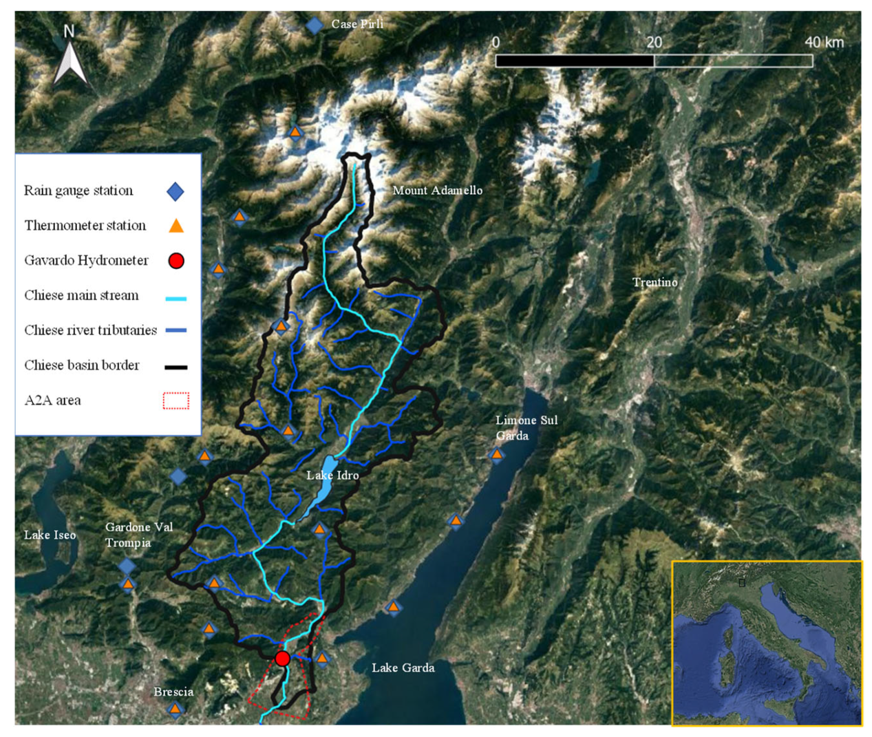
The study area refers to the river Chiese catchment where the Chiese mainstream has a length of about 121 km, originating from Mount Adamello in the Trentino region (Figure 1). The river Chiese is a large sub-tributary of the river Po, which is the longest river in Italy, playing a major role in the development of the country in terms of various economic activities. The area and perimeter of the catchment are roughly 971 km2 and 218 km, respectively, and the catchment includes 18 rain gauges and 15 thermometer stations. Along with the Gavardo hydrometer, these stations have contributed to the hydrological analysis and calibration of the river Chiese catchment. This work is carried out in the framework of the Lombardy Region CE4WE (Circular Economy for Water and Energy) project. The A2A (Water Utility) area in Figure 1 refers to the interest area of A2A managers for further water resource management activities based on estimated hydrological variables. The managers need to have a perspective on the future water availability of the catchment under an intermediate climate change scenario. For this purpose, the main assumption is that the only forcing factor for climate change is CO2 emission. Other human climate forces, such as changes in vegetation, soil, and water, as comprehensively mentioned in [24,25,26], are not considered in this study.
2.2. Hydrological Model
The river Chiese catchment is modeled using the TOPographic Kinematic AProximation and Integration TOPKAPI [27] software, enabling the user to set up a physically based and fully distributed hydrological model with fine space–time resolution ( cell sizes and one-hour time step). To achieve this, various GIS-based information, including the shapefiles of the catchment area, lakes, river network, and the gauged stations (thermometers, rain gauges, and hydrometers) are taken together with Digital Elevation Models (DEM). The maps of the soil and land-use units are collected from different sources, such as the environmental protection agency, ARPA (https://www.arpalombardia.it/Pages/Ricerca-Dati-ed-Indicatori.aspx, (accessed on 30 September 2022)), and the A2A water utility. The model is constructed in the GIS interface of TOPKAPI, MapWindow GIS, where a preprocessor is used to insert the input data, such as land use, soil parameters, and monthly temperature values. It is worth mentioning that the hydrological model has already been calibrated by another partner involved in the project. Therefore, the calibrated model was used in the context of the present work (more information about the TOPKAPI model, hydrological modeling, and calibration is provided in the Supplementary Materials).
2.3. Under Study Climate Models
A total of 10 coupled climate models (CMs) were investigated in the current study. The models were retrieved from the EURO-CORDEX CMIP5 (Coupled Model Intercomparison Project Phase Five) experiment [28] https://www.euro-cordex.net/, (accessed on 30 September 2022), and stored on the nodes of Earth System Grid Federation (ESGF), https://esg-dn1.nsc.liu.se/login/, (accessed on 30 September 2022).
The data were analyzed at the finest resolution, 0.11° (~12.5 km, EUR-11 referring to the models related to the European areas with the finest resolution) and considered for the historical period of 1971–2000 as a baseline. The used coupled Climate models are: CM5-RCA4, ECE-HIRH, ECE-RACM, ECE-RACMr12, ECE-RCA4, IPS-RCA4, Had-RACM, Had-RCA4, MPI-RCA4, and Nor-HIRH, which include three RCMs and six GCMs, the information of which is shown in Table 1 and Table 2. ECE-RACMr12 refers to the same model as ECE-RACM but considers a different realization (an ensemble experiment with different initial states from ECE-RACM).
2.3.1. Climate Models’ Performance Evaluations
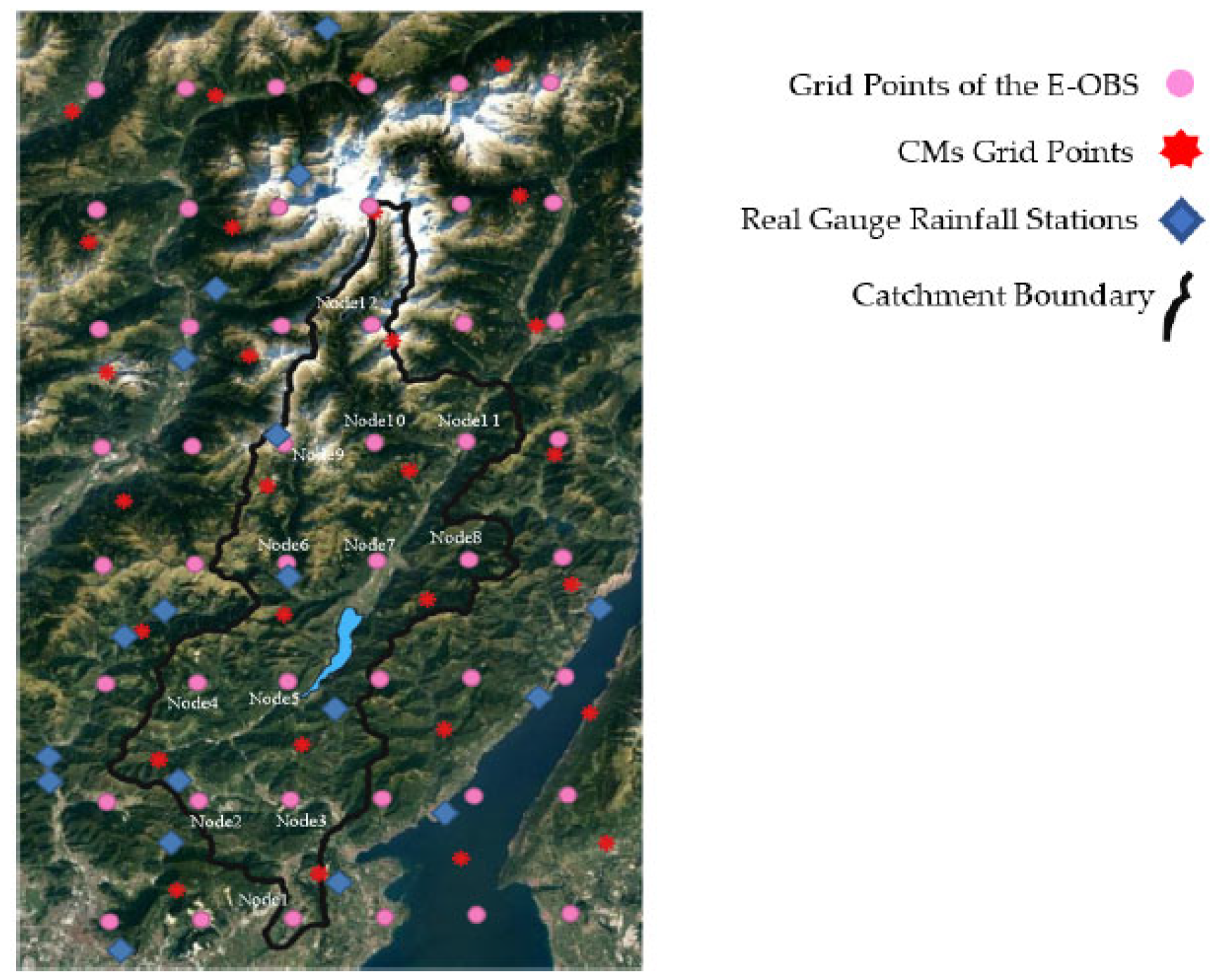
Work [23] demonstrated that for small-scale case studies, the averaged climatic variables over the catchment are a good surrogate of the whole catchment climate features, and they can be used for model evaluation and data projection purposes. Hence, together with the ensemble spatial analysis of climate models, this study used a weighted catchment approach, as used in [39], to evaluate the RCMs and impact models. In this approach, every grid point within the catchment border represents a fictitious weather station, called a node in Figure 2, playing the main role in the hydrological analysis of the catchment and in the RCM performance evaluation. To guarantee the good use of CMs’ grid points within the catchment, the longest and shortest east–west and north–south coordinates of real weather gauges were used for the operation of the CMs and finding the region grid points. That is why the outer catchment grid points were also visualized. In our study, all the regional climate models showed the grid points with the same coordinates for both hydro-climatological properties, temperature, and precipitation.
The models were evaluated in two important terms, uncertainty and error, which refer to two different concepts. Error and uncertainty could have an opposite conformity for a CM, meaning that the model could perform with low error but high uncertainty in reproducing or projecting particular catchment data, or vice versa. This is an important issue that has rarely received attention, and the current study provides a solution to overcome this challenge. For the uncertainty assessment, there are different factors affecting the uncertainties in the outputs, including uncertainty in the parameterization, initial and boundary conditions, greenhouse gas emissions scenarios, and models [40]. In this study, only uncertainty originating from the interaction of different coupled models was considered. For this purpose, the multi-model ensemble mean (MMEM) model is a new model resulting from averaging all the ensemble members. It was assumed that the MMEM model was the best in terms of covering the uncertainty shortcomings of the model’s outputs. For error assessment, the gridded observational-based daily dataset over the Europe domain called E-OBS was used against CM outputs to evaluate the performance of all the CMs. For this purpose, the last version of E-OBS was downloaded from the source https://surfobs.climate.copernicus.eu/dataaccess/access_eobs.php#datafiles (accessed on 30 September 2022) for both precipitation and temperature data over a 30-year control period, from 1971 to 2000. The finest spatial resolution of the E-OBS data (0.10°) was chosen, and the E-OBS grid points for both temperature and precipitation were visualized within the selection domain (Figure 2). As can be seen, 12 fictitious E-OBS stations are located within the catchment border. Due to the finer resolution of E-OBS data, the number of E-OBS grid points is more than that of the CM points within the catchment boundaries.
The monthly cumulative precipitation and monthly average temperature values are the target variables for evaluating the CMs. The monthly values of CMs are accessible directly from the source, while the daily E-OBS data should be aggregated over the month scale. In this study, the precipitation and temperature variables for a node are represented by , where x = P (precipitation) or T (temperature); , , ; and . refer to the number of months, years, E-OBS and CM nodes respectively. For every specific month and year, for example, (January) and (year 1971), the current methodology introduces a variable that provides the weighted average catchment value for the two target variables estimated by Equation (1).
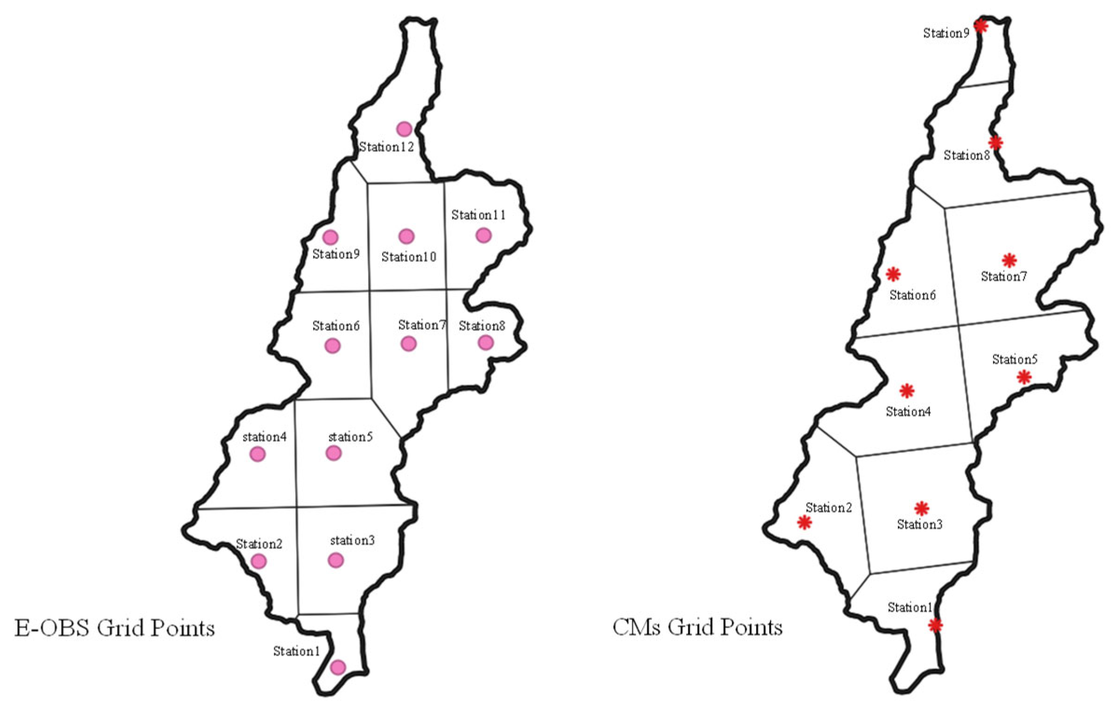
where represents the number of fictitious stations within the catchment, i.e., 9 and 12 for the CMs and E-OBS data. refers to the weight of every node calculated by the Thiessen polygons method such that the ratio of the Thiessen polygon area associated with the node to the total area of the catchment provides the weight of the corresponding node. The weights not only specify the significance of the role of the grid points in the hydrological analysis of the catchment, but also evaluate the suitability of CMs’ numerical schemes to the layout of the catchment in case they have different grid schemes.
Figure 3 and Table 3 show the Thiessen polygons and area information together with the weights and elevation of the fictitious stations (captured from the digital elevation model) for both the CM and E-OBS datasets.
Root Mean Square, Mean, and Standard Deviation Errors (RMSE, ME, and SDE, respectively) are the statistical error indices used to estimate the performance of the climate models in terms of validation. RMSE is calculated after ordering the climate model and E-OBS data associated with the benchmark period of nyears in ascending order, with the objective of evaluating the extent to which the cumulative frequency of the cumulative rainfall and temperature values obtained from the generic climate model is close to the corresponding cumulative frequency of the E-OBS data. For every specific month , for example , the monthly errors for the given precipitation and temperature variables of CM shown by () are calculated by Equation (2) as follows:
where represents the error of climate model for simulating month catchment variable ; defines the number of years in the control period, which is 30 in the current study; and and stand for the E-OBS and climate model precipitation or temperature values in month , respectively. The representative performance errors of the climate model , where varies from one to the number of CMs under study (the 10 downloaded models plus MMEM), are obtained for precipitation and temperature variables by Equation (3):
where represents the RMSE of the climate model in terms of precipitation and temperature simulations, respectively. Indeed, the representative error is equal to the average of all months’ RMSE values. Finally, represents the number of months in a year, which is 12. Other error indices are based on the mean and standard deviation of outputs calculated as follows:
Accordingly, the ME and SDE indices of catchment output are calculated for every climate model by Equations (6) and (7):
2.3.2. Ensemble Member Selection for Impact Models Assessment
There are different approaches in the literature for using climate models’ outputs in the hydrological and methodological models projecting future data and showing the impacts of climate change on the environment. The pre-defined CMs could achieve different ranks based on their error performance values. Moreover, the reliability of a model could change for target variable reproduction. For example, while a model shows a small error for generating precipitation data, it could have a high error for the temperature variable. Hence, depending on the type of impact model calculated by CMs’ outputs, the employment of CMs could change. For example, for the hydrological variables, precipitation is the main source of catchment recharge, and temperature plays the main role in evaporation and evapotranspiration. Hence, the reliable CM is the model with the lowest error for reproducing both weighted catchment precipitation and temperature variables. In this study, three weighted dimensionless error metrics are defined to rank the models in different aspects [23].
In the above-mentioned equations, and are weighting factors for precipitation and temperature errors, respectively, that satisfy . Equations (8)–(10) state the relative performance of different models in the reproduction of target variables. The neutral case is when and in the limiting case, and . The exact values of the weights for the hydrological impact models are obtained after sensitivity analyses and parameters tuning in the hydrological models.
Based on the error values, the CMs are ranked. The first ranked model is the most reliable one in terms of fitting the observed data. However, it may not be the best for covering uncertainty. The ideal case is the time when MMEM is ranked first, as it is the best model in terms of error and uncertainty. It is not guaranteed that the MMEM model always performs with the lowest error, and there could be a case when the MMEM model even has the highest error. In this instance, there is a tradeoff between two concepts of error and uncertainty, meaning that moving towards choosing the model covering uncertainty brings about a model with high error. To tackle this challenge, this study introduces an algorithm to select a subset of ensemble models that have average outputs which are unbiased and balanced for both error and uncertainty (see Figure 4).
2.3.3. Projection and Climate Change Impacts Assessment
There are 10 climate change impact model assessments in this study, as shown in Table 4. For all the models, the comparison periods are the 2070s in the future (2071–2080) vs. the 1990s in the historical period of 1991–2000. The aim is to assess the impacts of climate change on some hydro-climatological and hydrological variables under the RCP 4.5 climate change scenario. Every impact model is formed and calculated by its associated and suitable subset ensemble CMs. The relevant weight values for finding the best CMs are written in Table 4.
As we are dealing with a real project, all of the data generated by the best climate model or the best subset of the ensemble were modified by the bias correction factors to make all the simulations reliable for the decision-makers. There are many methods for the estimation of the bias correction factors [41]. This study used the linear-scaling method that has parsimony as its main advantage [10]. According to this method, the CM monthly precipitation data were corrected by multiplicative factors that bring the monthly means of corrected precipitation to match their observed values in the benchmark past period. On the other hand, the temperature data were adjusted through an additive term that brings the corrected average monthly mean temperature to equal the observed values in the benchmark past period. Thus, the corrections were the following for precipitation () and temperature (), respectively:
where denotes precipitation and denotes temperature, the overline indicates the mean operation, the subscript of E-OBS indicates the observed values, subscript stands for “historic period” (i.e., 1991–2000 in this study), and is the month index. The corrected historical and future data are given by the following equations:
where, in addition to the previously declared symbols, prime stands for “corrected value”, superscript indicates a future period (2071–2080 in this study), and is the year index.
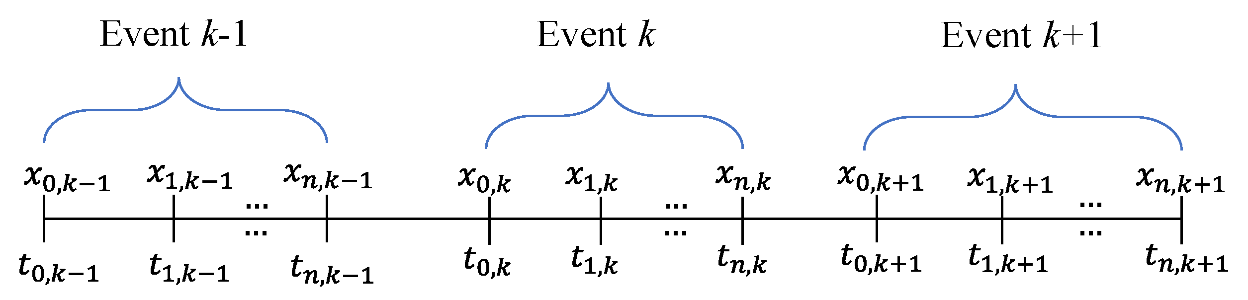
Rainfall event characteristics, including duration, intensity, and depth were assessed and compared. To accomplish this, the hourly data from the best-suited climate model were downloaded and modified by the bias correction factors. Independent rainfall events were selected based on an inter-event time of about 11 h, estimated based on the concentration and time of the catchment [42]. Figure 5 shows the time axis of three independent events where every event takes hours starting from time and ending at time . While and , all the time differences within the event and other subsequent events would be smaller or equal to the threshold. As the result, the duration, intensity, and depth of event are estimated by Equations (17)–(19).
where, , , and represent the length (hours), depth (mm), and intensity (mm/hours) of the rainfall event, . Here, the minimum temporal rainfall resolution was assumed to be one hour as the sub-hourly temporal resolution for the precipitation data is not provided by the climate models.
After calculating the lengths, depths, and intensities of rainfall events, they were compared between the future scenario and the historical period based on the cumulative frequency distribution graphs.
2.4. Linking Climate Model with the Hydrological Model
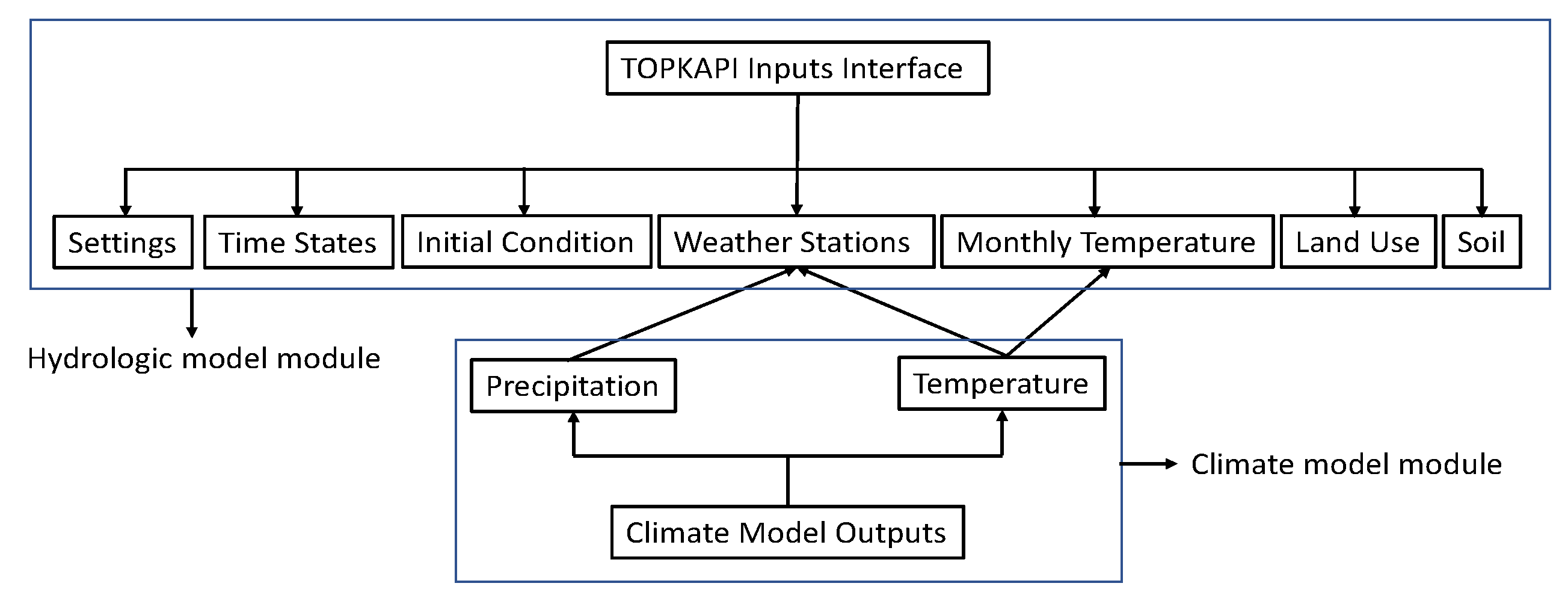
To link the climate model with the hydrologic model, the outputs of the climate models, precipitation, and temperature data were used as input to the hydrologic model. To accomplish this, the Chiese catchment was modeled through the TOPKAPI software, where the input variables and the parameters for the hydrologic model adjustments and simulations were controlled and inserted through the TOPKAPI user interface windows. The main receiver input windows are shown in Figure 6, where the climate model outputs are assembled into the weather stations and monthly temperature windows. As observed, two modules referring to hydrologic and climate models were linked only by two windows in the TOPKAPI Inputs Interface to complete the coupling process. The Weather Stations window includes the information on rain gauge and thermometer stations, including their coordinates, elevation, and hourly data values, whereas the Monthly Temperatures window contains the stations’ monthly average values for solving evapotranspiration equations over the hydrologic simulation period.
The fictitious stations were reconstructed in the Chiese catchment through the MapWindow GIS of TOPKAPI. The coordinates and elevation of the fictitious stations were obtained from the climate model file source and digital elevation model data.
All the inserted data values were modified by the bias correction factors before assembling. The coupling process was repeated for 1991–2000 and 2071–2080, considering greenhouse gas emission scenario 4.5 to estimate and compare the hydrological components of the catchment, including water discharge, percolation, and evapotranspiration. The input variables in the weather stations and monthly temperature windows were changed in the simulation, while the other parameters, such as soil type and land use, were assumed to be constant and invariable.
3. Results
3.1. Climate Model Rankings and Ensemble Member Selection for Impact Models
Table 5 compares the dimensionless errors obtained by Equations (8)–(10) and ranks, written in parenthesis, of the RCMs used for reconstructing the precipitation and temperature of the Chiese catchment over 1971–2000. Hy, P, and T refer to the error performances of the models in terms of suitability to the hydrology-based impacts simulations (models 7–10 in Table 4), precipitation-based impacts simulations (models 2–6 in Table 4), and temperature-based impacts simulations (model 1 in Table 4).
Overall, it can be seen that the MMEM model (the first-ranked uncertainty model) is not the best in any of the error competitions and, therefore, its outputs were not used for any impact model assessment. On the other hand, for a particular variable, the models are assigned different ranks based on different error metrics. For example, for hydrological variables, Had-RCA4 and Had-RACM commonly achieve the first rank in terms of RMSE and MPI-RCA4, ECE-RACMr12 achieve the first rank for mean and standard deviation errors. This begs the question of what the best subset of ensemble models is that could somehow cover the error and uncertainty of outputs for use in the impact models’ simulations. To tackle this, this study introduces the following novel method explained in Figure 4, making a fair balance between the error and uncertainty of outputs:
- The subset members of the ensemble set are those that have error values lower than the MMEM model (the highlighted models). For example, for hydrological variables, the three subset error metrics are as follows:
- The intersection between the three mentioned ensemble subset defines the CMs that should be used for impact assessment.where represents the multi-model set in which the members pass the three error metrics reliability tests. Finally, the output average of models in makes a model, , which was used for the hydrology impact model. Through this process, there is a balance between the uncertainty and error of the data. Repeating the process, the ensemble subset of the models for precipitation and temperature impact assessments were:
In addition to using multi-model outputs for climate change impact modeling, a single model’s outputs are used for this purpose to understand the uncertainty and error shortcomings of CMs’ outputs well. As mentioned earlier, some studies used a single model’s outputs, where the model is the best one in the error ranking. The current study introduces a strict error filtration to find the best solo model, which is the intersection of all three multi-model ensemble subsets, which is as follows:
To conclude, the CMs involved in any type of climate change impact modeling, as explained in Table 4, are summarized in Table 6. As observed, every type of impact model (past and future simulations of data under climate change scenario 4.5 and comparison between the results) is calculated two times, the first time by using multi-model outputs (the current study’s methodology) and the second time by the classical approach, using the best single model outputs. Through this activity, the signal and value uncertainties of the reconstructed and projected data are well assessed. The signal uncertainty shows the agreement of MM and SM about a trend (for example, increase, decrease, or neutral change in temperature). The value uncertainty shows the difference in the value of temperature change (for example, if catchment warming is certain, how much uncertainty is for centigrade catchment warming, 1 °C, 2 °C, or other values).
3.2. Climate Models Ensemble Evaluation
3.2.1. Model Evaluation Based on Weighted Catchment Value
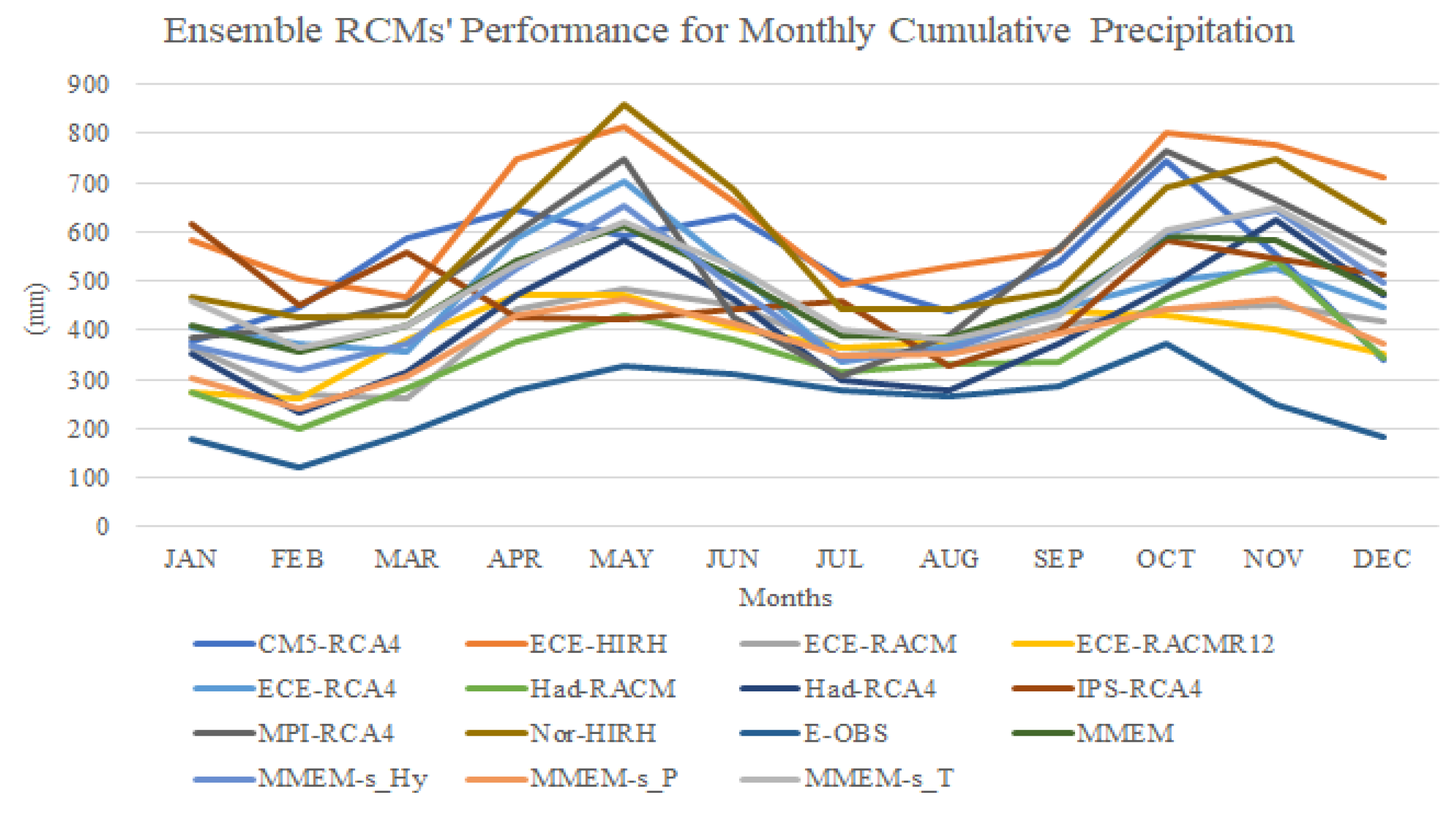
Figure 7 shows the performances of 14 RCMs in reproducing monthly cumulative precipitation data over the 1971–2000 period against E-OBS data. As observed, overestimation is obvious for all the RCMs’ performances, emphasizing the unreliability of RCMs’ outputs for use as inputs in the impact models. Hence, bias correction factors are needed for applying RCMs to the impact models’ simulations. In general, the errors for the summer months’ precipitation are lower than those related to the other seasons (Table S1). The maximum and minimum total average errors for all months are related to ECE-HIRH and Had-RACM with roughly 166% and 45%, respectively. The data generated from MMEM-s_P have moderate monthly errors where it achieves the second-best rank model in terms of the total average error values, 55%.
Figure 8 demonstrates the ensemble uncertainty evaluation of different RCMs. The model uncertainty in the outputs could originate from different sources, including GCM, RCM, or the coupled interaction of GCM-RCM [43]. In this study, only the GCM-RCM uncertainty was assessed, and the output deviation from the MMEM was considered to be a criterion for assessing the models’ uncertainty performances [44]. In Figure 8, the precipitation uncertainty for the summer months is lower than that for the other months. In terms of the total monthly average deviation, the highest and lowest uncertainties are related to ECE-HIRH and MMEM-s_T, with approximately 162 (mm) and 22 (mm), respectively (Table S2). Had-RACM, the lowest error model, shows roughly high uncertainty and more than MMEM-s_P, meaning that choosing the lowest error model does not always guarantee the lowest uncertainty.
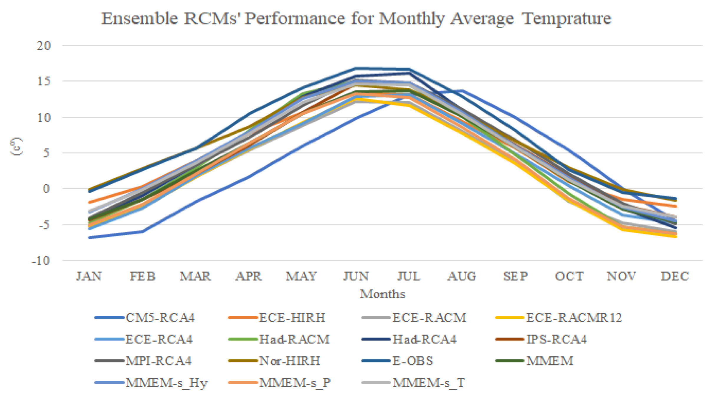
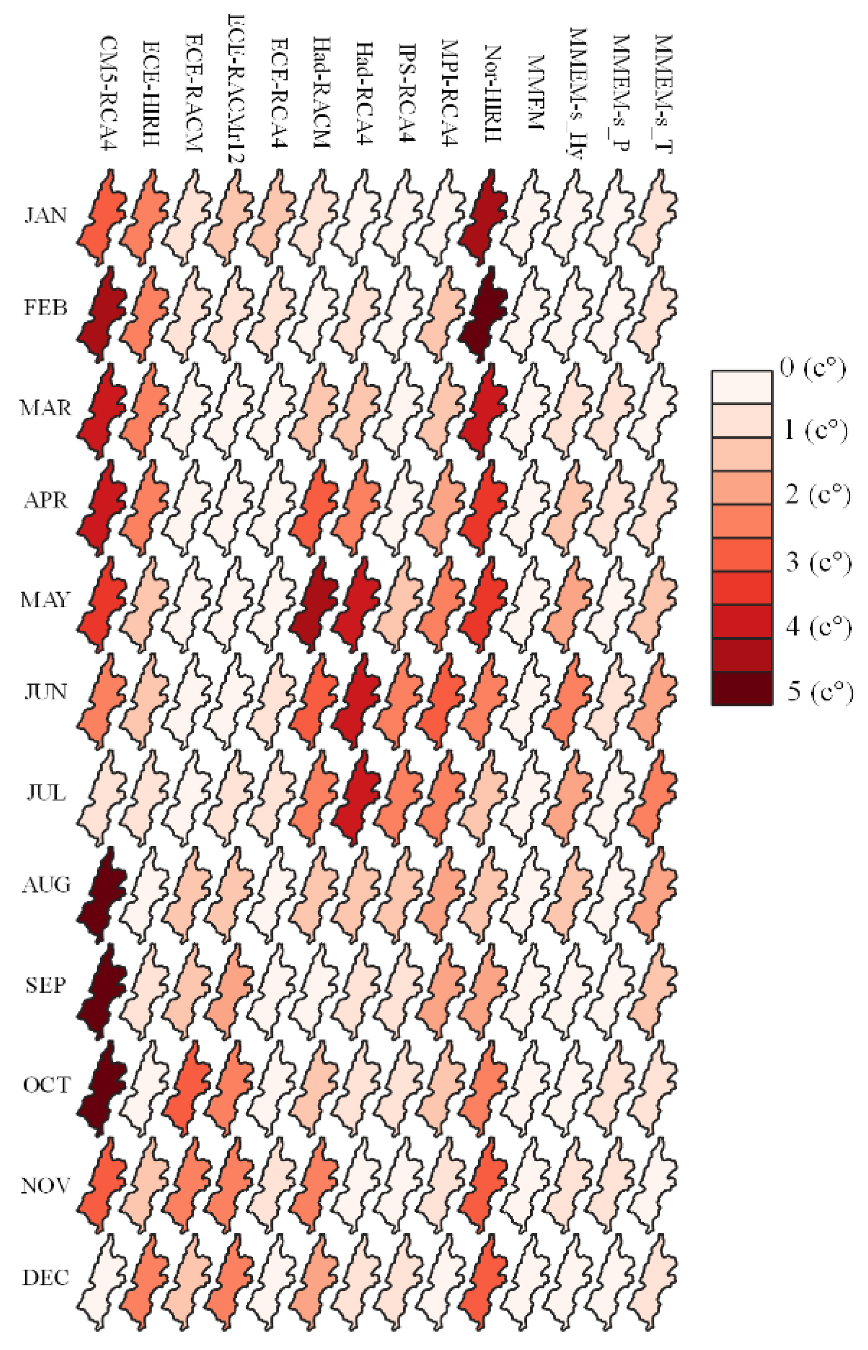
In Figure 9 and Figure 10, underestimation is well observed among all RCMs and for all monthly temperatures, except for CM5-RCA4, which has the highest total average error value of 4.9 °C (Table S3). In this regard, Nor-HIRH performs the best, with a total average error value of 1.12 °C, but it is not the best in terms of uncertainty, with a total average deviation of 2.80 °C (Table S4). Regarding uncertainty, the MMEM model is the best; however, it has quite a high error of 3.11 °C. MMEM-s_T strikes a good balance between the error and uncertainty values, with 2.29 and 0.99 °C, respectively.
In general, comparing uncertainty and error performances for precipitation and temperature properties shows that RCMs perform better when reconstructing temperature data than precipitation ones. Moreover, the subset ensemble selection approach, through a fair comparison of the two shortcomings of RCMs, can result in models (i.e., MMEM-s_T, MMEM-s_P, and MMEM-s_Hy) that have a good balance in error and uncertainty to avoid biased RCM selection and, therefore, highly inaccurate impact model results.
3.2.2. Model Evaluation Based on Spatial Analysis
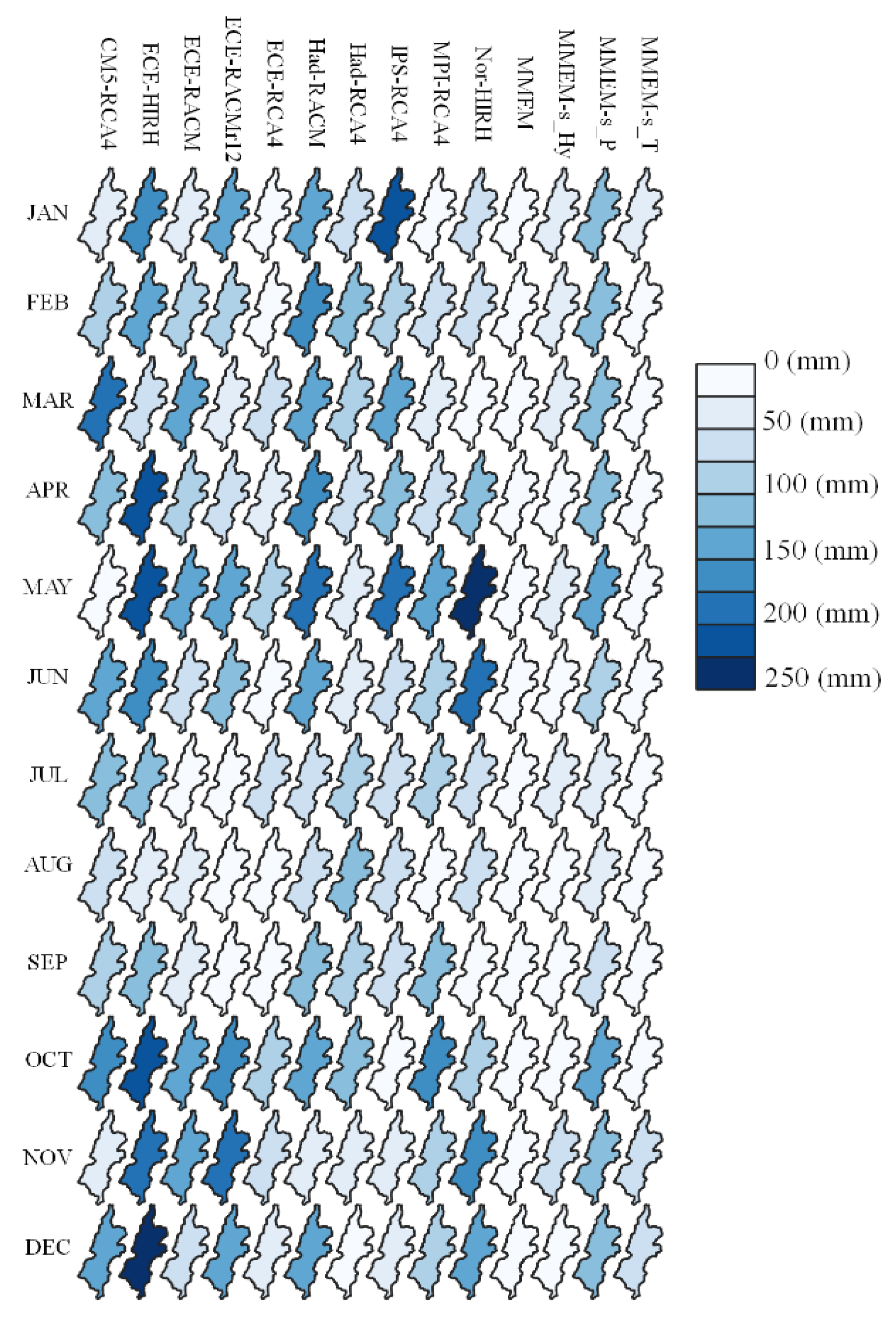
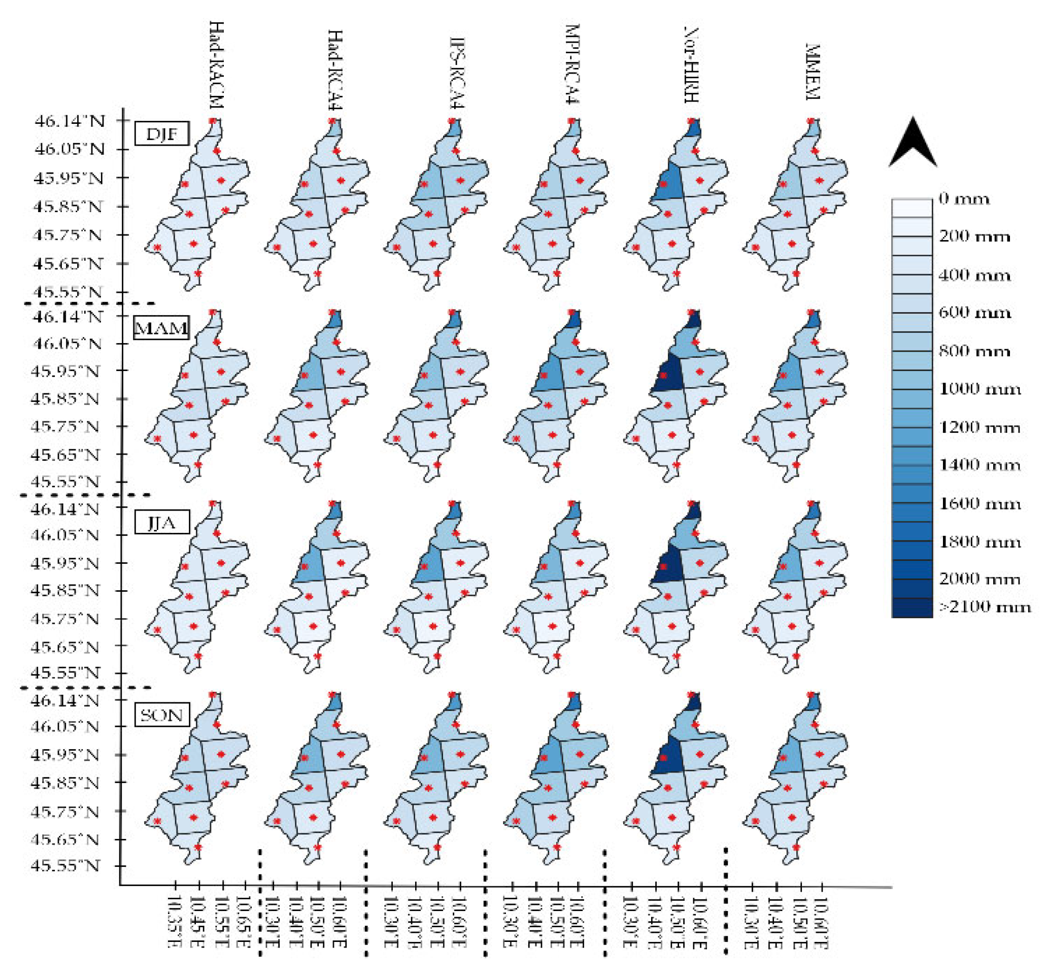
Figure 11 demonstrates the spatial variability of the seasonal cumulative precipitation values for winter season including the months of December, January, and February (DJF); spring season including the months of March, April, and May (MAM); summer season including the months of June, July, and August (JJA); and autumn including the months of September, October, and November (SON). In this regard, every fictitious station’s value is calculated and attributed to the associated Thiessen polygon. As observed, comparing the spatial distribution of precipitation from climate models with the one from E-OBS proves overestimation, which agrees with that shown for the catchment values in Figure 7. Among the climate models, the spatial variability of precipitation is higher for ECE-HIRH, CM5-RCA4, and Nor-HIRH than other models, where the fictitious stations with high elevation, particularly fictitious station 9, show a high amount of cumulative precipitation. Even though they achieved a low rank based on the dimensionless error assessment of a historical precipitation simulation (Table 5), they performed well when simulating the natural processes of air parcel cooling, condensing, and rain. This implies the poor performance of E-OBS when it comes to spatial variability analysis and the need for improvement of the observed data.
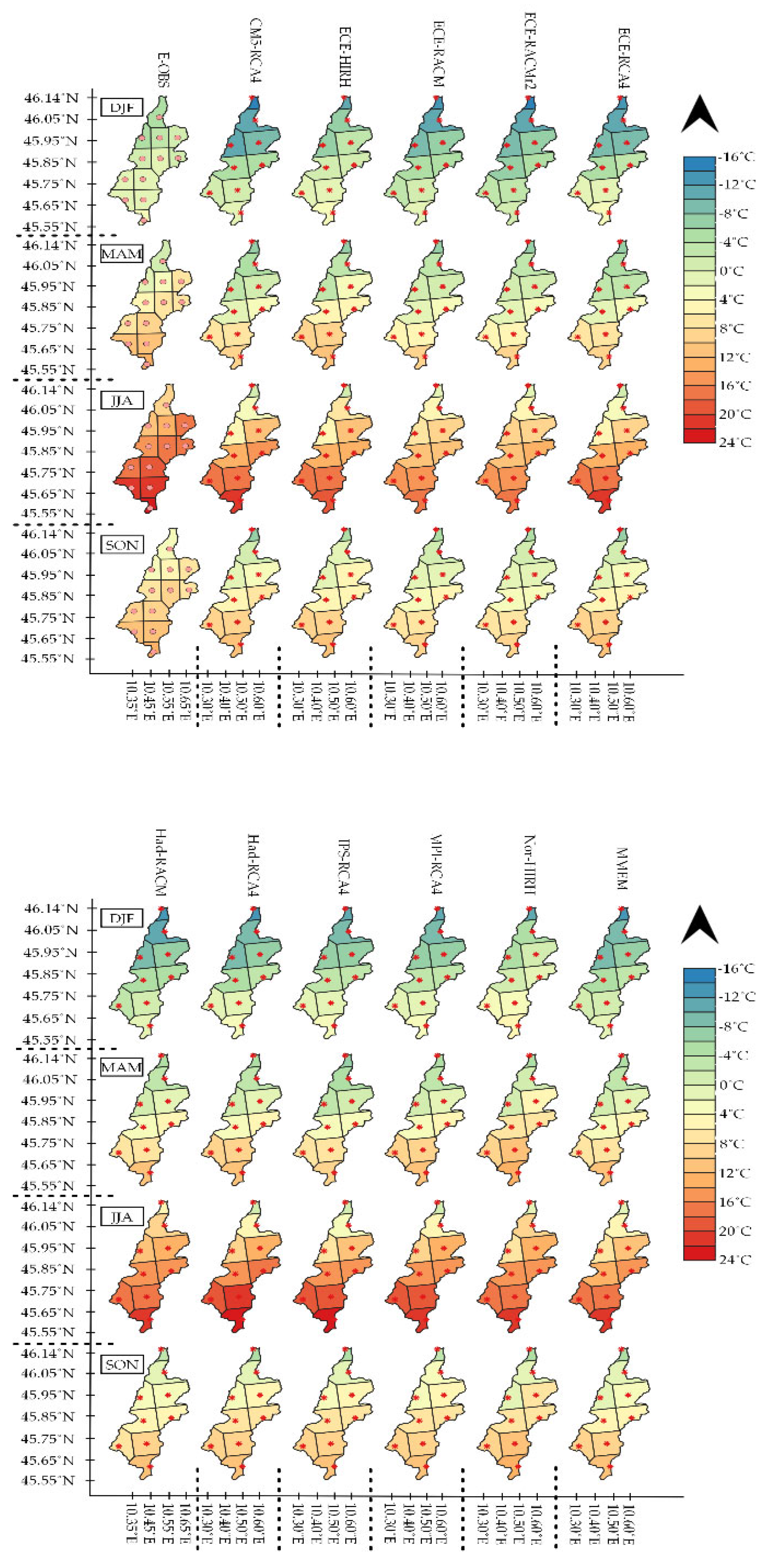
Figure 12 manifests the spatial variability of the seasonal average temperature estimated by the different models. As shown, spatial overestimation is clear in the seasonal temperature simulation performances of climate models. The spatial variability in the winter temperature is higher than in other seasons. As expected, the summer temperature is the highest, and all 12 models show a good correlation between the fictious stations’ elevations and associated temperatures such that moving from south to the north (lowest to the highest elevation) refers to a decrease in the seasonal temperature. Looking at the models, Nor-HIRH has the best-fitted temperature spatial distribution with the E-OBS one, while CM5-RCA4 is the poorest one, which is in a good agreement with their ranks in Table 5.
3.3. Impact Models’ Results
3.3.1. Temperature and Precipitation-Based Impact Models
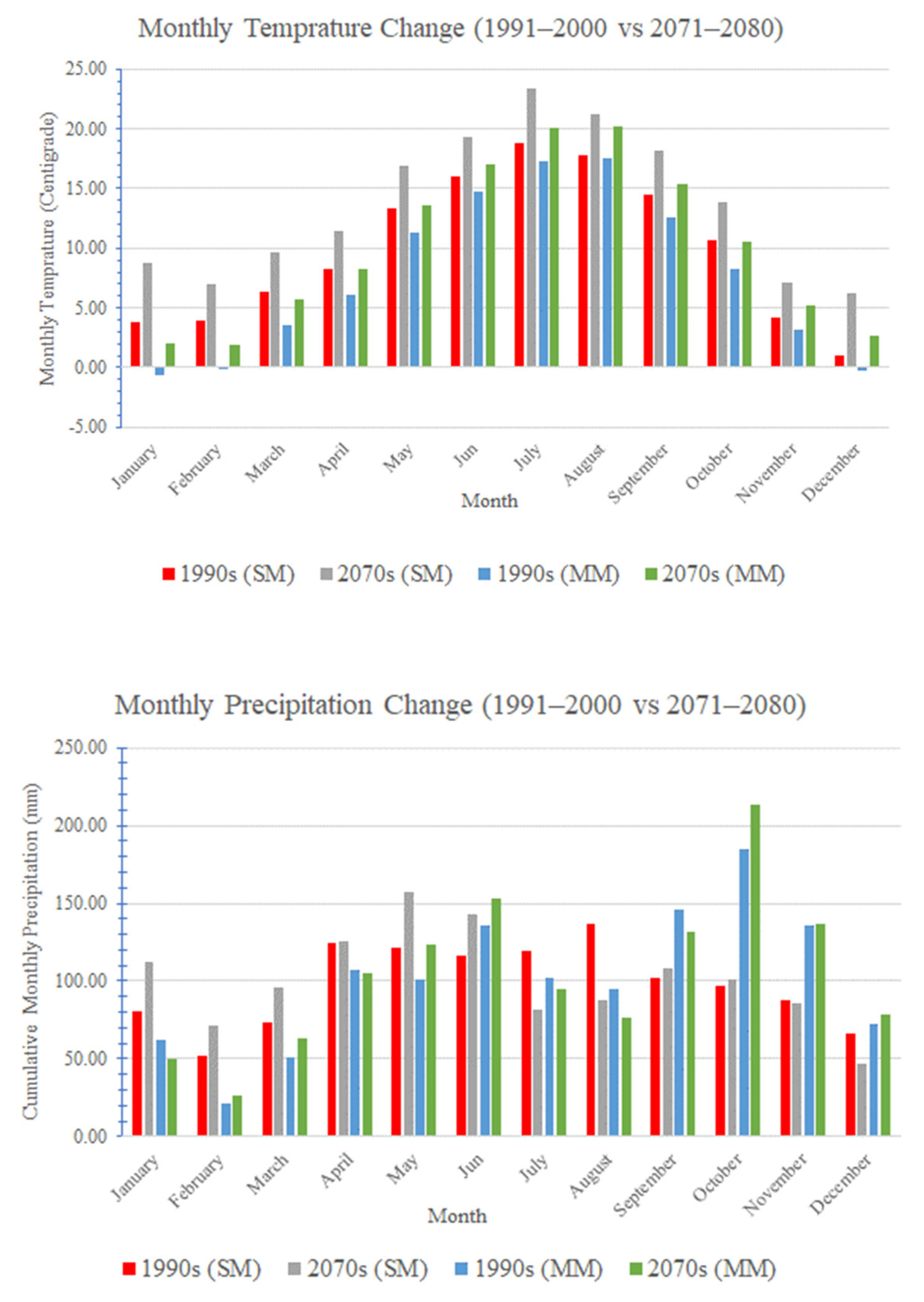
Figure 13 illustrates the variation in the weighted average Chiese catchment precipitation and temperature variables estimated over the two decades in the historical (1991–2000) and future (2071–2080) periods, where the results show how much the SM and MM approaches could make differences in the projection of data.
Overall, both SM and MM are in agreement concerning Chiese catchment warming (signal uncertainty is low as both models indicate temperature increase in the catchment), whereas there is not a clear trend for the precipitation values.
Looking at the details, regarding temperature, the coldest (December) and warmest (July) months remain the same over time for SM, while in the MM approach, the coldest months for the 1990s and 2070s are January and February, with about −0.65 °C and 1.93 °C, respectively, and the warmest month is August for both the past and future of the Chiese catchment. In general, the value uncertainty in projecting summer temperature data is lower than in winter ones. For example, the highest deviations between SM and MM are 4.47 °C and 6. 72 °C for the January months of the 1990s and 2070s, respectively, and the lowest deviations are 0.20 °C and 1.04 °C for the August months of the 1990s and 1970s, respectively (Table S5). To sum up, SM and MM projections for the average yearly increase in the temperature are about 3.69 °C and 2.41 °C, respectively, meaning 1.25 °C value uncertainty.
In terms of monthly precipitation for the Chiese catchment, there is not a clear signal by SM and MM. However, comparing the performance of SM and MM for historical reconstruction and future projection of precipitation data shows higher value uncertainty for the 2070s than the 1990s. In this regard, the highest and lowest deviations are related to the December of the 1990s and the January of the 2070s, with 6.35 mm and 62.48 mm, respectively (Table S6).
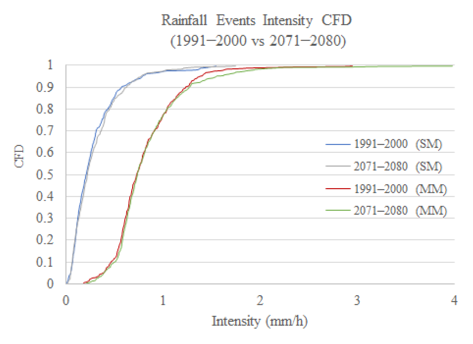
The projection of the precipitation characteristics was investigated for both historical and future data in Figure 14, showing the Gumbel cumulative frequency distribution (CFD) of three characteristics of rainfall events: depth, duration, and intensity for the 1990s and 2070s obtained using the SM and MM approaches. As observed, while SM points out that the future rainfall events would be with shorter duration, MM results show roughly the same duration for future and historical Chiese rainfall events. Hence, the signal and value uncertainties are high in this case. Regarding the depth, there is not a significant difference in the depths of the rainfall event behavior between the future and historical climate of Chiese for both SM and MM (the depth signal uncertainty is low, but the depth values uncertainty is high). At some knee points, there are considerable differences between the intensity of future and historical rainfall events. The same signals point out that the precipitation could fall with higher intensities in the future, particularly for the extreme ones. Assessing the value uncertainty in the results demonstrates a more dramatic deviation for duration property between SM and MM than depth and intensity properties. The interesting point is at the limit points of intensity and depth graphs where value and signal uncertainties move towards zero.
3.3.2. Hydrological Impact Models
Table 7 shows and compares the important water balance components at Gavardo station for the four simulations calculated through TOPKAPI. As can be seen, the decadal precipitation values for the future period (2071–2080) simulations are higher than the corresponding ones for the historical period (1991–2000) simulation. However, this does not refer to a considerable difference, and therefore, it is expected that the Chiese catchment will not face high variations in the total average yearly rainfall depth. Moreover, the precipitation deviations between SM and MM show higher uncertainty for the 2070s than the 1990s, with around 800 mm and 500 mm, respectively (signal certainty and values uncertainty).
As regards the percolation values, both SM and MM confirm a negligible change and deviation for decadal absolute and relative balances. The evapotranspiration values grow due to the catchment warming, and MM and SM show the same signal, that is, an increase in the relative decadal balance, about 2%, where value uncertainty is about 6%.
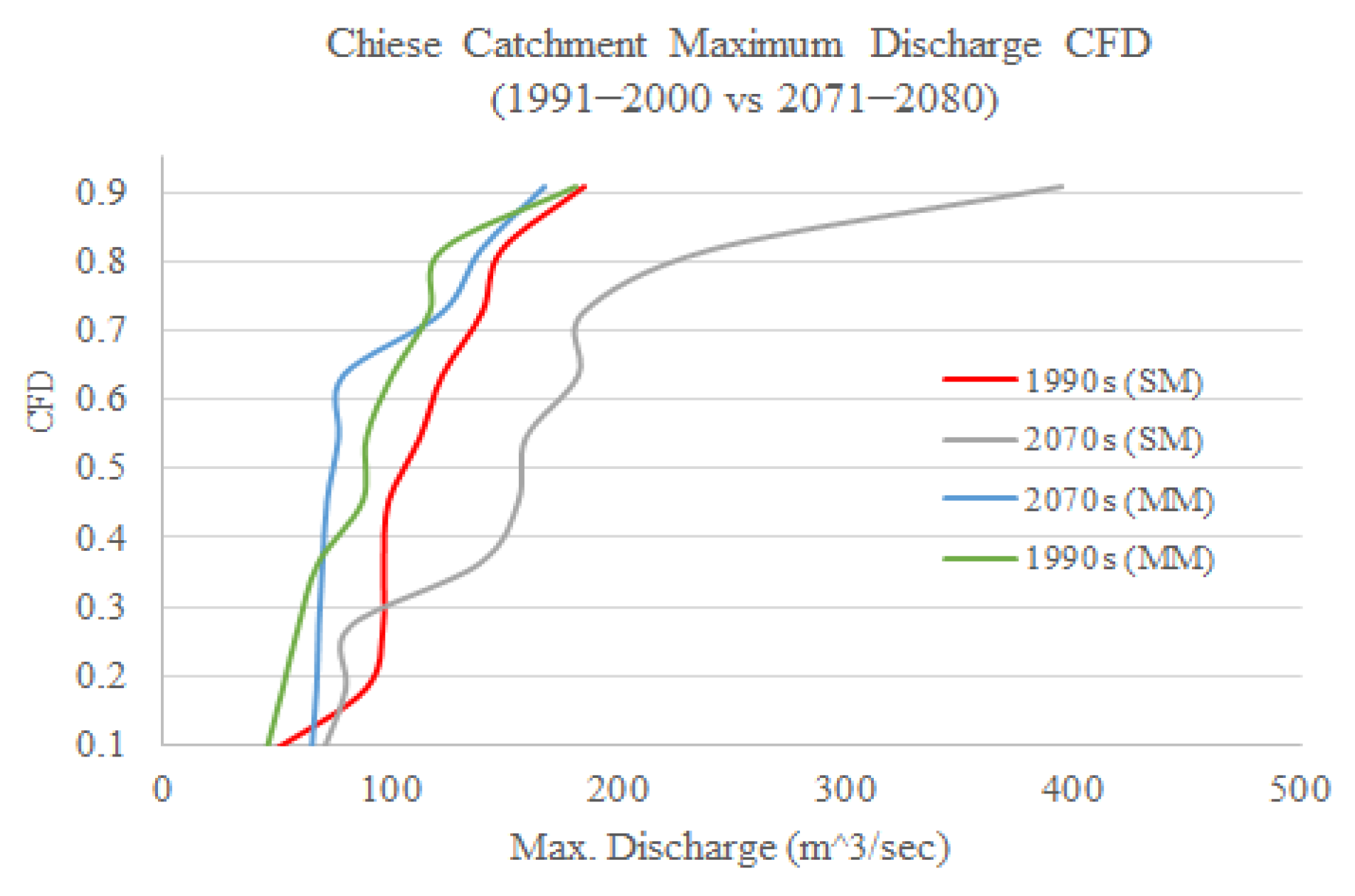
For the assessment of discharge variations, Table 7 shows an increase in the decadal discharge values for both SM and MM. However, the value uncertainties in the relative balance are similar to those related to the evapotranspiration component and higher than the percolation component by about 6%. Figure 15 compares the CFD of the yearly maximum discharge for the historical and future decades. While the results from SM are appreciable but not exorbitant increases for the maximum discharge values with 0.3 < CFD < 0.8, this is dramatically amplified for anomalies (values with CFD > 0.8). In this regard, MM does not project a clear trend for change in the maximum discharge of the Chiese catchment. With respect to the value uncertainty, in general, the deviation between SM and MM is higher for projected data than for past reconstruction. In this regard, the highest amount of value uncertainty is observed for extreme events in the future, calling for flood management and mitigation actions.
4. Discussion and Conclusions
Climate models’ performance reliability is under debate in the literature. In this context, the current study attempted to evaluate 10 ensemble EURO-CORDEX regional climate models plus 4 different combined climate models for solving a real project concerning the water availability of the River Chiese catchment. The evaluations were carried out considering the two common shortcomings of the models, which are error and uncertainty. For this purpose, together with the spatial analysis of the climate models’ outputs over the catchment, the weighted catchment value was calculated and used for different variables. The spatial analysis showed that for the small-scale catchments, the averaged catchment value could be considered an appropriate surrogate of the whole catchment climate for the evaluation and impact model assessments and calculations. High overestimation for the monthly cumulative precipitation was observed for all the under-RCMs’ outputs, whereas underestimation was observed among all the RCMs, except for CM5-RCA4, for the catchment average monthly temperature. Moreover, error and uncertainty were lower for the summer months than for the other seasons. In this regard, some dramatic error values were calculated, such as 312% for February precipitation obtained by ECE-HIRH. To address this weakness of RCMs, some studies introduced the multi-model ensemble mean (MMEM) as a reliable output for climate change assessment. However, our study showed a poor performance of MMEM on the river Chiese, while it nevertheless covers model-based uncertainty. To tackle this challenge, an algorithm was introduced, based on some simple set theories and three different error indices, to make some subsets of RCM ensemble able to balance error and uncertainty for every particular impact model simulation and assessment.
To apply climate models to project climatic data and assess the climate change in the catchment, some authors in the literature relied on the outputs of one climate model, which is usually the single best-performing model (SM). Yet, many criticized this approach and proposed an ensemble approach using multi-model (MM) outputs for covering the uncertainties in the reconstruction and projection of climatic data. The current study showed and compared the application of both approaches for assessing the climate change impacts on some hydro-climatological variables and uncertainties in this regard. The uncertainties were assessed in two terms, which were signal and value uncertainties. Signal uncertainty showed the agreement of models for the variables’ trends in the Chiese catchment, while value uncertainty demonstrated the differences in the measurements.
As a result of this, the impacts of climate change under scenario 4.5 were assessed between 1991–2000 and 2071–2080 for monthly precipitation, temperature, some rainfall features, and hydrological variables. Catchment warming is an obvious and certain issue (both SM and MM showed the same signal, which was temperature increase), while the precipitation signal is unclear and uncertain. The value and signal uncertainties for projecting summer temperature were lower than the winter temperature of the Chiese catchment.
Regarding rainfall event characteristics, SM predicts future rainfall events with higher intensities and lower durations where the depth remains the same. Whereas, MM approximately projects the same values for future catchment rainfall duration, depth, and intensity, meaning signal certainty for depth and signal uncertainty for intensity and duration features of rainfalls. The highest value of uncertainty is for the duration of rainfalls, while the uncertainty at the extreme points of depth and intensity features decreases. Regarding the hydrological variables, there is a certain result about rising evapotranspiration in the catchment, while the uncertainty in the decadal relative balance percolation of the catchment is negligible. There is an increase in the catchment discharge where a dramatic value uncertainty of about 350 m3/s is for the yearly projected maximum discharge.
To sum up, in agreement with previous researchers in the field, the current paper showed the unreliability of climate models’ outputs due to the high errors and uncertainty found in the results. However, an approach was introduced to choose the subset of ensemble models to moderate the shortcomings of RCMs’ outputs and to make the tradeoff between error and uncertainty of outputs when they conflict with each other. Having said that, the current study used some important simplifying assumptions (different uncertainty sources and human climate forcing interventions, vegetation, land use, and soil) that could have had appreciable impacts on the final results. Moreover, the under-study climate models were not as comprehensive as having all scenario simulations such as Scenario 2.6. The focus of future work will be on a comprehensive assessment of the vulnerability of the Chiese catchment against climate change [45], where more human climate interventions, greenhouse gas scenarios, and fewer assumptions will be considered in the evaluation of climate change impact models.
Supplementary Materials
The following supporting information can be downloaded at: https://www.mdpi.com/article/10.3390/w14233967/s1. Table S1: The RCMs’ error values (%) for weighted Chiese catchment cumulative precipitation calculated averagely for every month over 1971–2000 (error =); Table S2: The RCMs’ deviation values (mm), uncertainty, for weighted Chiese catchment cumulative precipitation calculated averagely for every month over 1971–2000, (deviation =); Table S3: The RCMs’ error values (°C) for weighted Chiese catchment temperature calculated averagely for every month over 1971–2000, (error =); Table S4: The RCMs’ deviation values (°C), uncertainty, for weighted Chiese catchment cumulative temperature calculated averagely for every month over 1971–2000, (deviation =); Table S5: The monthly temperature values (°C) for the historic (1991–200) and future periods (1971–2080, Scenario 4.5) obtained by the single model (SM) and multi model (MM) approaches as well as deviation values (°C), uncertainty, for every month (deviation =), , ; Table S6: The monthly precipitation values (mm) for the historic (1991–200) and future periods (1971–2080, Scenario 4.5) obtained by the single model (SM) and multi model (MM) approaches as well as deviation values (mm), uncertainty, for every month (deviation =); Figure S1: Conceptual layout of TOPKAPI; Figure S2: Water network and DEM of the Chiese catchment; Figure S3: Map of hierarchy of the channel network (the darker color corresponds to a higher degree in the hierarchy). The star sign represents the hydrometer of Gavardo station; Figure S4: Map of soil kind; every color is related to a code of a particular soil (shown in the legend) representing different parameters shown in Figure S5; Figure S5: Soil parameters used for the calibration including horizontal permeability at saturation (m/s), saturated water content, residual water content, soil depth (m), horizontal non-linear reservoir exponent, vertical permeability at saturation (m/s), vertical non-linear reservoir exponent; Figure S6: Output of TOPKAPI for the Chiese catchment. The first graph above shows the fit of simulated to observed water discharge at Gavardo (blue and red graphs indicate the observed and simulated discharges respectively). The other graphs report the other processes of the hydrological cycle, including percolation to groundwaters; Figure S7: Calibrated data in Initial Condition Window of user interface TOPKAPI for the Chiese catchment; Figure S8: Calibrated data in Land Use Window of user interface TOPKAPI for the Chiese catchment; Figure S9: Calibrated data in Temperature Window of user interface TOPKAPI for the Chiese catchment.
Author Contributions
Conceptualization, E.C. and S.T.; Formal analysis, A.M.; Investigation, A.M.; Methodology, A.M., S.T. and E.C.; Software, A.M.; Visualization, A.M.; Writing–original draft, A.M.; and Writing–review and editing, S.T., R.S. and E.C. All authors have read and agreed to the published version of the manuscript.
Funding
This work was financially supported by two funding sources including Regione Lombardia, POR-FESR 2014–2020–Call HUB Ricerca e Innovazione, Progetto 1139857 CE4WE: Approvvigionamento energetico e gestione della risorsa idrica nell’ottica dell’Economia Circolare (Circular Economy for Water and Energy) and DOC Fellowship of Austrian Academy of Sciences (ÖAW): AP845023.
Data Availability Statement
The data presented in this study are available on request from the corresponding author.
Acknowledgments
This work was carried out in the framework of the CE4WE (Circular Economy for Water and Energy) project, and the authors would like to send their deepest appreciation to all the holders, engineers and researchers involved in the project for their wonderful collaborations. Moreover, completion of the paper resulting from the project was financially supported by DOC Fellowship of Austrian Academy of Sciences and therefore the authors deeply appreciate this prestigious institute in Austria.
Conflicts of Interest
The authors declare no conflict of interest.
References
- Stocker, T. Climate Change 2013: The Physical Science Basis: Working Group I Contribution to the Fifth Assessment Report of the Intergovernmental Panel on Climate Change; Cambridge University Press: Cambridge, UK, 2014. [Google Scholar]
- Stone, M.C.; Hotchkiss, R.H.; Hubbard, C.M.; Fontaine, T.A.; Mearns, L.O.; Arnold, J.G. Impacts of Climate Change on Missouri Rwer Basin Water Yield 1. JAWRA J. Am. Water Resour. Assoc. 2001, 37, 1119–1129. [Google Scholar] [CrossRef]
- Frei, C.; Christensen, J.H.; Déqué, M.; Jacob, D.; Jones, R.G.; Vidale, P.L. Daily precipitation statistics in regional climate models: Evaluation and intercomparison for the European Alps. J. Geophys. Res. Atmos. 2003, 108, 4124. [Google Scholar] [CrossRef]
- Kunstmann, H.; Schneider, K.; Forkel, R.; Knoche, R. Impact analysis of climate change for an Alpine catchment using high resolution dynamic downscaling of ECHAM4 time slices. Hydrol. Earth Syst. Sci. 2004, 8, 1031–1045. [Google Scholar] [CrossRef] [Green Version]
- Piani, C.; Weedon, G.; Best, M.; Gomes, S.; Viterbo, P.; Hagemann, S.; Haerter, J. Statistical bias correction of global simulated daily precipitation and temperature for the application of hydrological models. J. Hydrol. 2010, 395, 199–215. [Google Scholar] [CrossRef]
- Park, C.; Min, S.-K.; Lee, D.; Cha, D.-H.; Suh, M.-S.; Kang, H.-S.; Hong, S.-Y.; Lee, D.-K.; Baek, H.-J.; Boo, K.-O. Evaluation of multiple regional climate models for summer climate extremes over East Asia. Clim. Dyn. 2016, 46, 2469–2486. [Google Scholar] [CrossRef]
- Peres, D.J.; Senatore, A.; Nanni, P.; Cancelliere, A.; Mendicino, G.; Bonaccorso, B. Evaluation of EURO-CORDEX (Coordinated Regional Climate Downscaling Experiment for the Euro-Mediterranean area) historical simulations by high-quality observational datasets in southern Italy: Insights on drought assessment. Nat. Hazards Earth Syst. Sci. 2020, 20, 3057–3082. [Google Scholar] [CrossRef]
- Tariku, T.B.; Gan, T.Y.; Li, J.; Qin, X. Impact of climate change on hydrology and hydrologic extremes of Upper Blue Nile River Basin. J. Water Resour. Plan. Manag. 2021, 147, 04020104. [Google Scholar] [CrossRef]
- Vezzoli, R.; Mercogliano, P.; Pecora, S.; Zollo, A.L.; Cacciamani, C. Hydrological simulation of Po River (North Italy) discharge under climate change scenarios using the RCM COSMO-CLM. Sci. Total Environ. 2015, 521, 346–358. [Google Scholar] [CrossRef]
- Peres, D.J.; Modica, R.; Cancelliere, A. Assessing Future Impacts of Climate Change on Water Supply System Performance: Application to the Pozzillo Reservoir in Sicily, Italy. Water 2019, 11, 2531. [Google Scholar] [CrossRef] [Green Version]
- Peres, D.; Caruso, M.; Cancelliere, A. Assessment of climate-change impacts on precipitation based on selected RCM projections. Eur. Water 2017, 59, 9–15. [Google Scholar]
- Shahi, N.K.; Das, S.; Ghosh, S.; Maharana, P.; Rai, S. Projected changes in the mean and intra-seasonal variability of the Indian summer monsoon in the RegCM CORDEX-CORE simulations under higher warming conditions. Clim. Dyn. 2021, 57, 1489–1506. [Google Scholar] [CrossRef]
- Ban, N.; Caillaud, C.; Coppola, E.; Pichelli, E.; Sobolowski, S.; Adinolfi, M.; Ahrens, B.; Alias, A.; Anders, I.; Bastin, S.; et al. The first multi-model ensemble of regional climate simulations at kilometer-scale resolution, part I: Evaluation of precipitation. Clim. Dyn. 2021, 57, 275–302. [Google Scholar] [CrossRef]
- Shahi, N.K.; Polcher, J.; Bastin, S.; Pennel, R.; Fita, L. Assessment of the spatio-temporal variability of the added value on precipitation of convection-permitting simulation over the Iberian Peninsula using the RegIPSL regional earth system model. Clim. Dyn. 2022, 59, 471–498. [Google Scholar] [CrossRef]
- Schmidli, J.; Goodess, C.; Frei, C.; Haylock, M.; Hundecha, Y.; Ribalaygua, J.; Schmith, T. Statistical and dynamical downscaling of precipitation: An evaluation and comparison of scenarios for the European Alps. J. Geophys. Res. Atmos. 2007, 112, D04105. [Google Scholar] [CrossRef] [Green Version]
- Endris, H.S.; Omondi, P.; Jain, S.; Lennard, C.; Hewitson, B.; Chang’a, L.; Awange, J.; Dosio, A.; Ketiem, P.; Nikulin, G. Assessment of the performance of CORDEX regional climate models in simulating East African rainfall. J. Clim. 2013, 26, 8453–8475. [Google Scholar] [CrossRef]
- Mascaro, G.; White, D.D.; Westerhoff, P.; Bliss, N. Performance of the CORDEX—Africa regional climate simulations in representing the hydrological cycle of the Niger River basin. J. Geophys. Res. Atmos. 2015, 120, 12425–12444. [Google Scholar] [CrossRef]
- Diasso, U.; Abiodun, B.J. Drought modes in West Africa and how well CORDEX RCMs simulate them. Theor. Appl. Climatol. 2017, 128, 223–240. [Google Scholar] [CrossRef]
- Wu, F.-T.; Wang, S.-Y.; Fu, C.-B.; Qian, Y.; Gao, Y.; Lee, D.-K.; Cha, D.-H.; Tang, J.-P.; Hong, S.-Y. Evaluation and projection of summer extreme precipitation over East Asia in the Regional Model Inter-comparison Project. Clim. Res. 2016, 69, 45–58. [Google Scholar] [CrossRef]
- Senatore, A.; Hejabi, S.; Mendicino, G.; Bazrafshan, J.; Irannejad, P. Climate conditions and drought assessment with the Palmer Drought Severity Index in Iran: Evaluation of CORDEX South Asia climate projections (2070–2099). Clim. Dyn. 2019, 52, 865–891. [Google Scholar] [CrossRef]
- Soriano, E.; Mediero, L.; Garijo, C. Selection of bias correction methods to assess the impact of climate change on flood frequency curves. Water 2019, 11, 2266. [Google Scholar] [CrossRef] [Green Version]
- Um, M.J.; Kim, Y.; Kim, J. Evaluating historical drought characteristics simulated in CORDEX East Asia against observations. Int. J. Climatol. 2017, 37, 4643–4655. [Google Scholar] [CrossRef]
- Deidda, R.; Marrocu, M.; Caroletti, G.; Pusceddu, G.; Langousis, A.; Lucarini, V.; Puliga, M.; Speranza, A. Regional climate models’ performance in representing precipitation and temperature over selected Mediterranean areas. Hydrol. Earth Syst. Sci. 2013, 17, 5041–5059. [Google Scholar] [CrossRef] [Green Version]
- Hossain, F.; Arnold, J.; Beighley, E.; Brown, C.; Burian, S.; Chen, J.; Madadgar, S.; Mitra, A.; Niyogi, D.; Pielke, R., Sr. Local-to-regional landscape drivers of extreme weather and climate: Implications for water infrastructure resilience. J. Hydrol. Eng. 2015, 20, 02515002. [Google Scholar] [CrossRef] [Green Version]
- Council, N.R.; Committee, C.R. Radiative Forcing of Climate Change: Expanding the Concept and Addressing Uncertainties; National Academies Press: Washington, DC, USA, 2005. [Google Scholar]
- Kabat, P.; Claussen, M.; Dirmeyer, P.A.; Gash, J.H.; de Guenni, L.B.; Meybeck, M.; Hutjes, R.W.; Pielke, R.A., Sr.; Vorosmarty, C.J.; Lütkemeier, S. Vegetation, Water, Humans and the Climate: A New Perspective on an Internactive System; Springer Science & Business Media: Berlin, Germany, 2004. [Google Scholar]
- Liu, Z.; Todini, E. Towards a comprehensive physically-based rainfall-runoff model. Hydrol. Earth Syst. Sci. 2002, 6, 859–881. [Google Scholar] [CrossRef]
- Jacob, D.; Petersen, J.; Eggert, B.; Alias, A.; Christensen, O.B.; Bouwer, L.M.; Braun, A.; Colette, A.; Déqué, M.; Georgievski, G. EURO-CORDEX: New high-resolution climate change projections for European impact research. Reg. Environ. Chang. 2014, 14, 563–578. [Google Scholar] [CrossRef]
- Voldoire, A.; Sanchez-Gomez, E.; Salas y Mélia, D.; Decharme, B.; Cassou, C.; Sénési, S.; Valcke, S.; Beau, I.; Alias, A.; Chevallier, M. The CNRM-CM5. 1 global climate model: Description and basic evaluation. Clim. Dyn. 2013, 40, 2091–2121. [Google Scholar] [CrossRef] [Green Version]
- Hazeleger, W.; Severijns, C.; Semmler, T.; Ştefănescu, S.; Yang, S.; Wang, X.; Wyser, K.; Dutra, E.; Baldasano, J.M.; Bintanja, R. EC-Earth: A seamless earth-system prediction approach in action. Bull. Am. Meteorol. Soc. 2010, 91, 1357–1364. [Google Scholar] [CrossRef] [Green Version]
- Dufresne, J.-L.; Foujols, M.-A.; Denvil, S.; Caubel, A.; Marti, O.; Aumont, O.; Balkanski, Y.; Bekki, S.; Bellenger, H.; Benshila, R. Climate change projections using the IPSL-CM5 Earth System Model: From CMIP3 to CMIP5. Clim. Dyn. 2013, 40, 2123–2165. [Google Scholar] [CrossRef] [Green Version]
- Collins, W.; Bellouin, N.; Doutriaux-Boucher, M.; Gedney, N.; Halloran, P.; Hinton, T.; Hughes, J.; Jones, C.; Joshi, M.; Liddicoat, S. Development and evaluation of an Earth-System model–HadGEM2. Geosci. Model Dev. 2011, 4, 1051–1075. [Google Scholar] [CrossRef] [Green Version]
- Giorgetta, M.A.; Jungclaus, J.; Reick, C.H.; Legutke, S.; Bader, J.; Böttinger, M.; Brovkin, V.; Crueger, T.; Esch, M.; Fieg, K. Climate and carbon cycle changes from 1850 to 2100 in MPI-ESM simulations for the Coupled Model Intercomparison Project phase 5. J. Adv. Model. Earth Syst. 2013, 5, 572–597. [Google Scholar] [CrossRef]
- Bentsen, M.; Bethke, I.; Debernard, J.B.; Iversen, T.; Kirkevåg, A.; Seland, Ø.; Drange, H.; Roelandt, C.; Seierstad, I.A.; Hoose, C. The Norwegian Earth System Model, NorESM1-M–Part 1: Description and basic evaluation of the physical climate. Geosci. Model Dev. 2013, 6, 687–720. [Google Scholar] [CrossRef]
- Iversen, T.; Bentsen, M.; Bethke, I.; Debernard, J.; Kirkevåg, A.; Seland, Ø.; Drange, H.; Kristjansson, J.; Medhaug, I.; Sand, M. The Norwegian earth system model, NorESM1-M–Part 2: Climate response and scenario projections. Geosci. Model Dev. 2013, 6, 389–415. [Google Scholar] [CrossRef] [Green Version]
- Strandberg, G.; Bärring, L.; Hansson, U.; Jansson, C.; Jones, C.; Kjellström, E.; Kupiainen, M.; Nikulin, G.; Samuelsson, P.; Ullerstig, A. CORDEX Scenarios for Europe from the Rossby Centre Regional Climate Model RCA4; SMHI: Norrköping, Sweden, 2015. [Google Scholar]
- Van Meijgaard, E.; Van Ulft, L.; Van de Berg, W.; Bosveld, F.; Van den Hurk, B.; Lenderink, G.; Siebesma, A. The KNMI Regional Atmospheric Climate Model RACMO, Version 2.1; Citeseer: Utrecht, Netherlands, 2008. [Google Scholar]
- Christensen, O.B.; Drews, M.; Christensen, J.H.; Dethloff, K.; Ketelsen, K.; Hebestadt, I.; Rinke, A. The HIRHAM Regional Climate Model; Version 5 (Beta); Danish Climate Centre, Danish Meteorological Institute: Copenhagen, Denmark, 2007. [Google Scholar]
- Minaei, A.; Todeschini, S.; Sitzenfrei, R.; Creaco, E. A Weighted Catchment View Approach for Evaluation of Euro Cordex Regional Climate Models. In Proceedings of the Copernicus Meetings, Vienna, Austria, 23–27 May 2022. [Google Scholar]
- Christensen, O.B.; Kjellström, E. Partitioning uncertainty components of mean climate and climate change in a large ensemble of European regional climate model projections. Clim. Dyn. 2020, 54, 4293–4308. [Google Scholar] [CrossRef]
- Teutschbein, C.; Seibert, J. Bias correction of regional climate model simulations for hydrological climate-change impact studies: Review and evaluation of different methods. J. Hydrol. 2012, 456–457, 12–29. [Google Scholar] [CrossRef]
- Giandotti, M. Previsione delle Piene e delle Magre dei Corsi D’Acqua; Memorie e Studi Idrografici, VIII. Servizio Idrografico Italiano: Rome, Italy, 1934; p. 1071933. [Google Scholar]
- Déqué, M.; Somot, S.; Sanchez-Gomez, E.; Goodess, C.; Jacob, D.; Lenderink, G.; Christensen, O. The spread amongst ENSEMBLES regional scenarios: Regional climate models, driving general circulation models and interannual variability. Clim. Dyn. 2012, 38, 951–964. [Google Scholar] [CrossRef] [Green Version]
- Christensen, O.B.; Kjellström, E. Filling the matrix: An ANOVA-based method to emulate regional climate model simulations for equally-weighted properties of ensembles of opportunity. Clim. Dyn. 2022, 58, 2371–2385. [Google Scholar] [CrossRef]
- O’Brien, K.; Eriksen, S.; Nygaard, L.P.; Schjolden, A. Why different interpretations of vulnerability matter in climate change discourses. Clim. Policy 2007, 7, 73–88. [Google Scholar] [CrossRef]
Figure 1.
The river Chiese catchment, located at the northeast of Italy.

Figure 2.
The grid points of the E-OBS (pink circles) in the Chiese domain. Blue diamonds and red stars refer to the real gauge rainfall stations and CMs grid points. E-OBS grid points within the catchment are called nodes.
Figure 2.
The grid points of the E-OBS (pink circles) in the Chiese domain. Blue diamonds and red stars refer to the real gauge rainfall stations and CMs grid points. E-OBS grid points within the catchment are called nodes.

Figure 3.
The Thiessen polygons of the fictitious stations of E-OBS and CMs’ data, left and right.

Figure 4.
Algorithm for balancing ensemble members between error and uncertainty for an impact model assessment.
Figure 4.
Algorithm for balancing ensemble members between error and uncertainty for an impact model assessment.

Figure 5.
The time axis of three independent rainfall events.

Figure 6.
TOPKAPI user interface windows for inserting the inputs.

Figure 7.
Ensemble model for the under-study climate models’ performances in the reconstruction of monthly cumulative precipitation data of Chiese catchment (for finding the exact error values, please refer to Table S1).
Figure 7.
Ensemble model for the under-study climate models’ performances in the reconstruction of monthly cumulative precipitation data of Chiese catchment (for finding the exact error values, please refer to Table S1).

Figure 8.
Under study climate models’ outputs deviation from grand ensemble mean (MMEM) for the reconstruction of monthly cumulative precipitation of the Chiese catchment (for the exact values of uncertainty, please refer to Table S2).
Figure 8.
Under study climate models’ outputs deviation from grand ensemble mean (MMEM) for the reconstruction of monthly cumulative precipitation of the Chiese catchment (for the exact values of uncertainty, please refer to Table S2).

Figure 9.
Ensemble model for the under-study climate models’ performances in the reconstruction of monthly average temperature data of Chiese catchment (for finding the exact error values, please refer to Table S3).
Figure 9.
Ensemble model for the under-study climate models’ performances in the reconstruction of monthly average temperature data of Chiese catchment (for finding the exact error values, please refer to Table S3).

Figure 10.
Under study climate models’ output deviation from grand ensemble mean (MMEM) for the reconstruction of the monthly average temperature of Chiese catchment (for the exact values of uncertainty, please refer to Table S4).
Figure 10.
Under study climate models’ output deviation from grand ensemble mean (MMEM) for the reconstruction of the monthly average temperature of Chiese catchment (for the exact values of uncertainty, please refer to Table S4).

Figure 11.
Ensemble model for analyzing spatial variability of 12 models, 10 RCMs, E-OBS, and MMEM models for reconstructing of historical, 1971–2000, seasonal cumulative precipitation values. The red and pink nodes in the figures refer to the fictitious stations of climate and E-OBS models.
Figure 11.
Ensemble model for analyzing spatial variability of 12 models, 10 RCMs, E-OBS, and MMEM models for reconstructing of historical, 1971–2000, seasonal cumulative precipitation values. The red and pink nodes in the figures refer to the fictitious stations of climate and E-OBS models.


Figure 12.
Ensemble model for analyzing spatial variability of 12 models, 10 RCMs, E-OBS, and MMEM models for reconstruction of historical, 1971–2000, seasonal average temperature values. The red and pink nodes in the figures refer to the fictitious stations of climate and E-OBS models.
Figure 12.
Ensemble model for analyzing spatial variability of 12 models, 10 RCMs, E-OBS, and MMEM models for reconstruction of historical, 1971–2000, seasonal average temperature values. The red and pink nodes in the figures refer to the fictitious stations of climate and E-OBS models.

Figure 13.
Temperature and precipitation changes in the Chiese catchment under Scenario 4.5 through the single-model (SM) and multi-model (MM) approaches.
Figure 13.
Temperature and precipitation changes in the Chiese catchment under Scenario 4.5 through the single-model (SM) and multi-model (MM) approaches.

Figure 14.
The rainfall event characteristics of Chiese catchment, duration, depth, and intensity change under Scenario 4.5 obtained by single and multi-model approaches.
Figure 14.
The rainfall event characteristics of Chiese catchment, duration, depth, and intensity change under Scenario 4.5 obtained by single and multi-model approaches.


Figure 15.
The yearly maximum discharge CFD for Chiese catchment over the historical and future periods obtained by single-model and multi-model approaches.
Figure 15.
The yearly maximum discharge CFD for Chiese catchment over the historical and future periods obtained by single-model and multi-model approaches.


Table 1.
GCMs were used in the current study and in the EURO-CORDEX ensemble experiment.
| Model Name | Abbreviation | Reference | Developer Institution |
|---|---|---|---|
| CNRM-CERFACS-CNRM-CM5 | CM5 | Voldoire, Sanchez-Gomez [29] | National Centre for Meteorological Research |
| ICHEC-EC-EARTH | ECE | Hazeleger, Severijns [30] | Irish Centre for High-End Computing EC-Earth Consortium, Europe |
| IPSL-IPSL-CM5A-MR | IPS | Dufresne, Foujols [31] | Institute Pierre Simon Laplace |
| MOHC-HadGEM2-ES | Had | Collins, Bellouin [32] | Met Office Hadley Centre |
| MPI-M-MPI-ESM-LR | MPI | Giorgetta, Jungclaus [33] | Max Planck Institute for Meteorology |
| NCC-NorESM1-M | Nor | [34,35] | Norwegian Earth System Model |
Table 2.
RCMs were used in the current study and in the EURO-CORDEX ensemble experiment.
| Model Name | Abbreviation | Reference | Institution |
|---|---|---|---|
| SMHI-RCA4 | RCA4 | Strandberg, Bärring [36] | Swedish Meteorological and Hydrological Institute, Rossby Centre |
| KNMI-RACM022E | RACM | van Meijgaard, Van Ulft [37] | Royal Netherlands Meteorological Institute, De Bilt, the Netherlands |
| DMI-HRIHHAM5 | HRIH | Christensen, Drews [38] | Danish Meteorological Institute |
Table 3.
The Thiessen polygon area of fictitious stations together with their weights.
| E-OBS | CMs | |||||
|---|---|---|---|---|---|---|
| Factitious Station ID | Area (km2) | Elevation (m) | Weight | Area (km2) | Elevation (m) | Weight |
| 1 | 32.82 | 228 | 0.034 | 77.14 | 313 | 0.079 |
| 2 | 73.53 | 497 | 0.076 | 101.95 | 626 | 0.105 |
| 3 | 106.06 | 354 | 0.109 | 146.69 | 837 | 0.151 |
| 4 | 76.35 | 1117 | 0.079 | 144.89 | 1535 | 0.149 |
| 5 | 112.00 | 564 | 0.115 | 104.70 | 1471 | 0.108 |
| 6 | 91.52 | 992 | 0.094 | 102.30 | 1737 | 0.105 |
| 7 | 101.80 | 658 | 0.105 | 159.84 | 1147 | 0.165 |
| 8 | 56.44 | 1284 | 0.058 | 109.40 | 2630 | 0.113 |
| 9 | 66.00 | 2186 | 0.068 | 24.10 | 3012 | 0.025 |
| 10 | 86.18 | 1918 | 0.089 | |||
| 11 | 76.79 | 656 | 0.079 | |||
| 12 | 91.52 | 2501 | 0.094 | |||
| Summation | 971.01 | 1.00 | 971.01 | 1.00 | ||
Table 4.
Different impact models in the current study and relevant weight values for the associated climate models.
Table 4.
Different impact models in the current study and relevant weight values for the associated climate models.
| Impact Model ID | Explanation | ||
|---|---|---|---|
| 1 | Change in average monthly temperature values | 0 | 1 |
| 2 | Change in cumulative monthly precipitation values | 1 | 0 |
| 3 | Change in rainfall events’ depth | 1 | 0 |
| 4 | Change in rainfall events’ duration | 1 | 0 |
| 5 | Change in rainfall events’ intensity | 1 | 0 |
| 6 | Change in decadal balanced cumulative precipitation | 1 | 0 |
| 7 | Change in decadal balanced cumulative discharge | 0.5 | 0.5 |
| 8 | Change in decadal balanced cumulative percolation | 0.5 | 0.5 |
| 9 | Change in decadal balanced cumulative evapotranspiration | 0.5 | 0.5 |
| 10 | Change in yearly maximum discharge | 0.5 | 0.5 |
Table 5.
Different dimensionless errors and ranks of climate models for Chiese catchment for different types of impact models.
Table 5.
Different dimensionless errors and ranks of climate models for Chiese catchment for different types of impact models.
| Model ID | Model Name | Hy | P | T | ||||||
|---|---|---|---|---|---|---|---|---|---|---|
| ME | SDE | RMSE | ME | SDE | RMSE | ME | SDE | RMSE | ||
| 1 | CM5-RCA4 | 12% (6) | 10% (4) | 11% (5) | 12% (6) | 10% (4) | 11% (7) | 12% (8) | 10% (5) | 11% (6) |
| 2 | IPS-RCA4 | 9% (4) | 13% (6) | 9% (3) | 9% (5) | 13% (6) | 10% (6) | 8% (4) | 11% (6) | 8% (3) |
| 3 | Had-RCA4 | 7% (2) | 10% (4) | 7% (1) | 6% (3) | 9% (3) | 7% (3) | 6% (2) | 11% (6) | 7% (2) |
| 4 | Had-RACM | 7% (2) | 6% (2) | 7% (1) | 4%(1) | 4% (1) | 5% (1) | 9% (5) | 7% (3) | 9% (4) |
| 5 | MPI-RCA4 | 6% (1) | 10% (4) | 8% (2) | 12% (6) | 13% (6) | 12% (8) | 7% (3) | 9% (4) | 7% (2) |
| 6 | ECE-RACM | 9% (4) | 6% (2) | 10% (4) | 6% (3) | 4% (1) | 6% (2) | 13% (9) | 7% (3) | 13% (7) |
| 7 | ECE-RACMr12 | 9% (4) | 5% (1) | 10% (4) | 5% (2) | 4% (1) | 5% (1) | 14% (10) | 5% (1) | 13% (7) |
| 8 | ECE-HIRH | 12% (6) | 11% (5) | 11% (5) | 16% (8) | 17% (7) | 15% (9) | 7% (3) | 6% (2) | 7% (2) |
| 9 | ECE-RCA4 | 11% (5) | 9% (3) | 10% (4) | 8% (4) | 9% (3) | 9% (5) | 11% (7) | 10% (5) | 11% (6) |
| 10 | Nor-HIRH | 8% (3) | 9% (3) | 8% (2) | 13% (7) | 12% (5) | 12% (8) | 3% (1) | 7% (3) | 4% (1) |
| 11 | MMEM | 10% (5) | 11% (5) | 9% (3) | 9% (5) | 5% (2) | 8% (4) | 10% (6) | 19% (7) | 10% (5) |
Table 6.
Ensemble subset of CMs for climate change impact modelling through two approaches of multi-model (MM) and single model (SM).
Table 6.
Ensemble subset of CMs for climate change impact modelling through two approaches of multi-model (MM) and single model (SM).
| Impact Model ID | MM | SM |
|---|---|---|
| 1 | ||
| 2 | ||
| 3 | ||
| 4 | ||
| 5 | ||
| 6 | ||
| 7 | ||
| 8 | ||
| 9 | ||
| 10 |
Table 7.
Changes in the Hydrologic Water Balance components of Chiese catchment under Scenario 4.5 over the historical and future periods, obtained by single-model and multi-model approaches.
Table 7.
Changes in the Hydrologic Water Balance components of Chiese catchment under Scenario 4.5 over the historical and future periods, obtained by single-model and multi-model approaches.
| Simulation Name | Precipitation (mm) | Discharge | Percolation | Evapotranspiration | |||
|---|---|---|---|---|---|---|---|
| Balance (mm) | Balance (%) | Balance (mm) | Balance (%) | Balance (mm) | Balance (%) | ||
| 90s (SM) | 11,729.29 | 9130.33 | 73.03% | 554.67 | 4.44% | 2619.13 | 20.95% |
| 90s (MM) | 12,294.38 | 8720.95 | 67.19% | 564.72 | 4.35% | 3465.68 | 26.7% |
| 70s (SM) | 12,190.20 | 9512.52 | 72.53% | 541.21 | 4.13% | 2894.41 | 22.07% |
| 70s (MM) | 12,953.37 | 8900.18 | 66.00% | 568.08 | 4.22% | 3862.16 | 28.64% |
Publisher’s Note: MDPI stays neutral with regard to jurisdictional claims in published maps and institutional affiliations. |
© 2022 by the authors. Licensee MDPI, Basel, Switzerland. This article is an open access article distributed under the terms and conditions of the Creative Commons Attribution (CC BY) license (https://creativecommons.org/licenses/by/4.0/).
Share and Cite
MDPI and ACS Style
Minaei, A.; Todeschini, S.; Sitzenfrei, R.; Creaco, E. Ensemble Evaluation and Member Selection of Regional Climate Models for Impact Models Assessment. Water 2022, 14, 3967. https://doi.org/10.3390/w14233967
AMA Style
Minaei A, Todeschini S, Sitzenfrei R, Creaco E. Ensemble Evaluation and Member Selection of Regional Climate Models for Impact Models Assessment. Water. 2022; 14(23):3967. https://doi.org/10.3390/w14233967
Chicago/Turabian StyleMinaei, Amin, Sara Todeschini, Robert Sitzenfrei, and Enrico Creaco. 2022. "Ensemble Evaluation and Member Selection of Regional Climate Models for Impact Models Assessment" Water 14, no. 23: 3967. https://doi.org/10.3390/w14233967
Note that from the first issue of 2016, this journal uses article numbers instead of page numbers. See further details here.