1. Introduction
Cut-off walls change the seepage direction, extend the seepage path and then mitigate groundwater seepage [
1,
2,
3]. Therefore, cut-off walls are usually used to reduce seepage flow under hydraulic structures (dams or dikes) [
4,
5,
6,
7] and inflow into an excavation pit [
8,
9,
10,
11,
12,
13,
14,
15]. As shown in
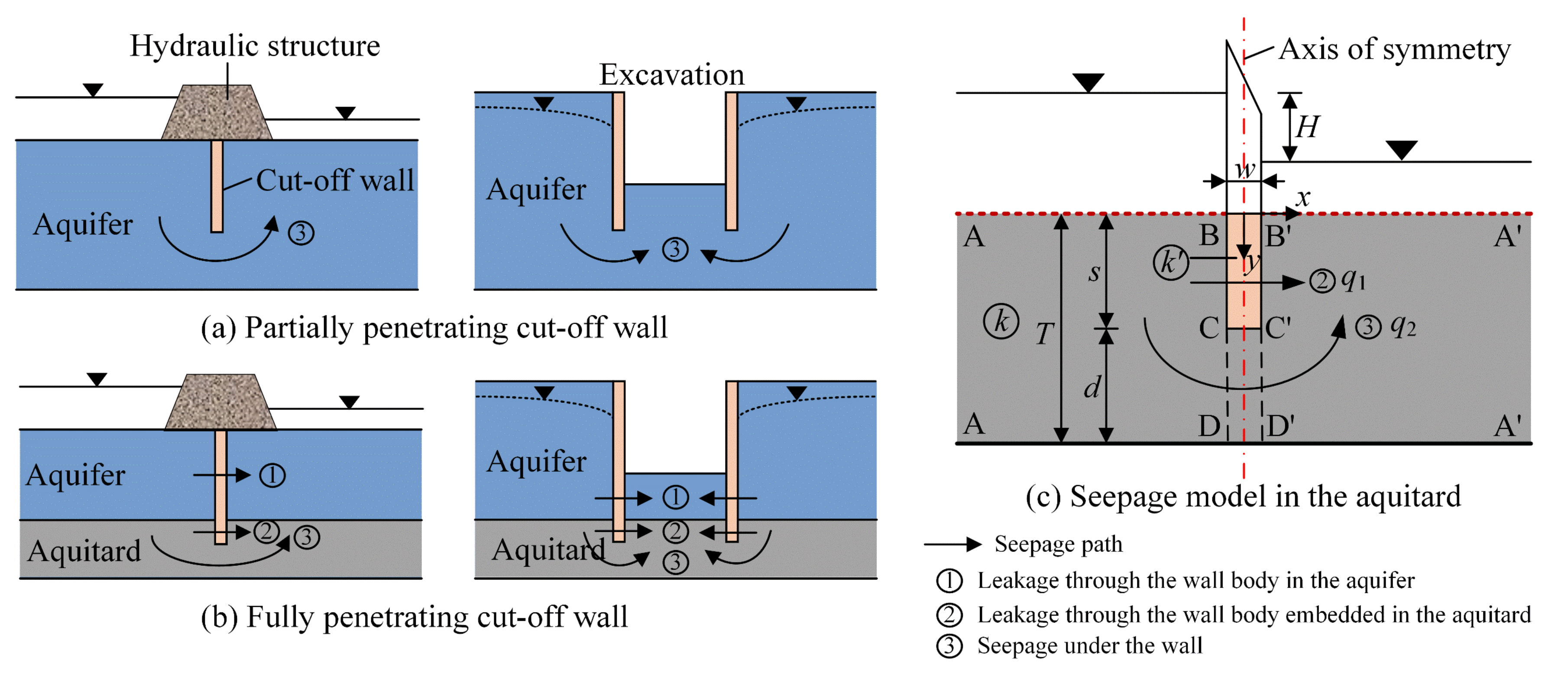
Figure 1, a partially penetrating cut-off wall is adopted when the aquifer is of a large thickness, whereas a fully penetrating cut-off wall is used when the thickness of the aquifer is small.
Different types of cut-off walls are used in practice and include the following: sheet- pile walls, deep-mixing piles, jet-grouting columns, secant piles, and diaphragm walls. They are usually defined as barriers with very low permeability. However, the cut-off walls have defects and cracks due to construction defects, and leakage through the body of wall is prone to occur [
1,
16]. For instance, overlapping jet-grouting columns and secant piles may display diameter variability and/or vertical deviation induced by soil heterogeneity and uncertainty of mechanical drilling, which can ultimately cause apertures in the wall body [
17,
18,
19,
20,
21]. Other construction techniques, such as diaphragm walls, pile walls and sheet piles, although made of reinforced concrete, may leak at the joints (interlocks) [
1,
5,
7]. Some concrete cut-off walls have construction defects due to improper construction methods or material selection, resulting in the effective hydraulic conductivity of the wall being two to three orders of magnitude larger than the anticipated value [
4,
22]. The effective hydraulic conductivity of a cut-off wall refers to quantity of leakage through a unit area of the wall driven by a unit hydraulic gradient when considering the effects of wall materials, wall defects and cracks. Defects and cracks in cut-off walls may significantly shorten the seepage pathway, leading to an increase in flow rate. Therefore, a cut-off wall is always permeable, and its effective hydraulic conductivity often appears to be much larger than the anticipated value.
A partially penetrating cut-off wall does not fully penetrate the aquifer. Although the wall is permeable, its permeability is generally much smaller than the aquifer permeability, and thus the seepage mainly occurs under the wall (see
Figure 1a). Many studies have been conducted for this seepage analysis, such as fundamental analytical solutions for the seepage beneath a dam with a partially penetrating cut-off wall [
23,
24,
25,
26] and analysis of inflow into a deep foundation pit considering the effect of such type of wall [
27].
A fully penetrating cut-off wall fully penetrates the aquifer and is embedded in an underlying aquitard to a certain depth. In engineering practice, this type of wall is commonly regarded as an impermeable barrier, and thus the wall is expected to fully obstruct the seepage flow under hydraulic structures or provide closed compartments for the excavation of foundation pits [
8,
28,
29]. However, a fully penetrating cut-off wall is always slightly permeable. Its permeability may be much smaller than the aquifer permeability, but not necessarily compared to the underlying aquitard. When leakage through the wall body occurs, the effective hydraulic conductivity of the wall may not differ much from the hydraulic conductivity of the aquitard. In addition, significant flow may also occur through the bedrock joints under the wall when the wall is embedded in jointed rocks [
4,
5]. Thus, groundwater seepage with this type of wall occurs through three paths: leakage through the wall body in the aquifer, leakage through the wall body embedded in the aquitard, and seepage under the wall, as depicted in
Figure 1b. Seepage through the first path can be simply treated as one-dimensional flow [
30,
31]. However, due to the mutual influence of seepage through the latter two paths, the seepage problem is complicated and still needs to be studied.
In general, the permeability of the aquifer is much higher than that of the underlying aquitard. Thus, the head change within a small area near the cut-off wall in the aquifer can be overlooked [
32]. Then, seepage flow near the cut-off wall in the aquitard can be modelled by the seepage model, as illustrated in
Figure 1c.
Internal permeable boundary conditions are formed along both sides of the cut-off wall, due to the difference in the permeability between the wall and the aquitard. The internal permeable boundary conditions make the seepage model in
Figure 1c difficult to solve exactly. In previous studies, the cut-off wall was simplified to an impermeable sheet pile with no thickness [
23,
24], or the effect of the wall permeability or thickness on the seepage was considered separately [
26,
32]. Based on the assumption that cut-off walls are impermeable sheet piles with no thickness, Aravin and Numerov [
23] listed fundamental analytical solutions for the seepage through foundations beneath dams. When the wall penetration depth in the aquitard is zero and the dam width is equal to the wall thickness, the exact solution for the seepage under the wall can be obtained from this study. Wang [
26] derived an exact solution for the seepage through foundation beneath a dam with an impermeable cut-off wall, and the effect of the wall thickness on the seepage was studied. When the dam width is equal to the wall thickness, the seepage under the cut-off wall can be solved exactly. Nevertheless, the leakage through the wall body cannot be counted. Yakimov and Kacimov [
32] assumed that the cut-off wall was infinitely thin and derived exact solutions for the leakage through the wall body and seepage under the wall. The effect of the wall permeability on the seepage was studied. Although the wall thickness is small compared to the thickness of the foundation soil, it has a considerable effect on the seepage under the wall and thus should be considered in the seepage analysis [
26].
Few studies have considered the effects of the wall permeability and thickness on seepage at the same time. For the seepage model in
Figure 1c, if the cut-off wall fully penetrates the aquitard, exact and approximate solutions for the leakage through the wall body can be obtained from the study of Anderson [
31]. However, for more-general cases in which the cut-off wall is just embedded in the aquitard to a certain depth, the seepage problem has not been studied.
Thus, an analytical method is proposed for the seepage in the aquitard (including the leakage through the wall body and seepage under the wall) while simultaneously considering the effects of the wall permeability and thickness. The proposed method is based on the seepage model in
Figure 1c. Analytical formulas for flow rate and head value are obtained by superposition of drawdowns of two exact models, namely, the model with only leakage through the wall body and that with only seepage under the wall, respectively. Exact solutions are quoted or derived for the two exact models. To facilitate an engineering application, approximate models of the exact models are introduced and their solutions are applied to the analytical formulas. Meanwhile, the exact models are used as calibration tools. Then, the accuracy and applicability of the proposed method are verified compared with the numerical method. The proposed method can be degenerated into models that do not need superposition of drawdowns for three special cases: the wall penetration depth in the aquitard is zero, the cut-off wall fully penetrates the aquitard, and the wall permeability is very small compared to the aquitard permeability. The degradation formulas are verified by the analytical solutions in the studies of Aravin and Numerov [
23], Anderson [
31], and Wang [
26], respectively. Finally, the effects of the wall permeability and thickness on the flow rate are discussed compared with the analytical solutions of Wang [
26] and Yakimov and Kacimov [
32], respectively.
2. Analytical Method
The analytical model is shown in
Figure 1c. The aquitard is of thickness
T and hydraulic conductivity
k. The cut-off wall is of thickness
w, effective hydraulic conductivity
k’, and penetration depth
s. The thickness of the aquitard under the wall is
d =
T −
s. The segments AB and A’B’ are the pervious boundaries and the total head drop from AB to A’B’ is
H. The segment ADD’A’ is the impervious boundary.
The analytical method is developed based on four assumptions:
Two-dimensional steady seepage flow is studied, and the analytical model is symmetrical taking the centerline of the cut-off wall as the axis of symmetry.
The aquitard extends horizontally infinitely on both sides of the cut-off wall.
The permeability ratio k’/k ≤ 1 is discussed here.
The flow is approximated as one-dimensional and horizontal within the regions BCC’B’ and CDD’C’. The flow in a vertical leaky wall can be assumed to be normal to the wall, which is demonstrated by Strack et al. [
33]. Here, BCC’B’ is a leaky wall region with permeability of
k’, and CDD’C’ can be taken as a wall region with permeability of
k.
Meanwhile, the superposition principle is applied to obtain drawdown. Superposition states that for a linear system, the effect of multiple stimuli on a system is the summation of the effect of each stimulus on the system [
34]. For the seepage problem in
Figure 1c, the drawdown
S is caused by quantity of leakage through the wall body (flow rate
q1) and quantity of seepage under the wall (flow rate
q2) simultaneously. Based on the superposition principle, the drawdown
S is the sum of one part caused by
q1 (noted as
S(q1)) and another part caused by
q2 (noted as
S(q2)). The relationship can be obtained as
S =
S(q1) +
S(q2). The
S(q2) and
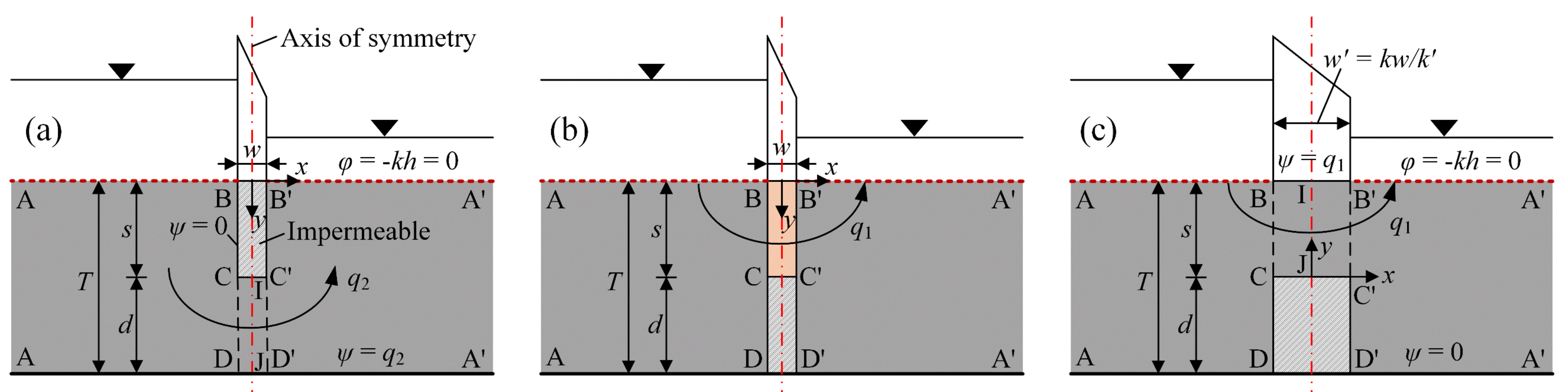
S(q1) can be obtained by two simpler models in
Figure 2a and
Figure 2b, respectively, which are called the model with only seepage under the wall and the one with only leakage through the wall body. The quantity of seepage under the wall in
Figure 2a is identical to
q2, and the quantity of leakage through the wall body in
Figure 2b is identical to
q1.
The drawdown S(x, y) of each point in the region ABCDA is the difference between the upstream head hAB and the head value h(x, y): S(x, y) = hAB − h(x, y). The drawdown S(x, y) of each point in the region A’B’C’D’A’ is the difference between the downstream head hA’B’ and the head value h(x, y): S(x, y) = hA’B’ − h(x, y).
The permeability and thickness of the cut-off wall are simultaneously considered in the analytical method. The permeability ratio can reach k’/k >1 sometimes (e.g., in the case that deep mixing piles are embedded in clay of weak permeability), but k’/k ≤ 1 is discussed in this study.
The purpose of the analytical method is to estimate the flow rates
q1,
q2, and the total flow rate
q (=
q1 +
q2) in
Figure 1c.
2.1. Mathematic Expression for Flow Rates
Assuming that the flow is one-dimensional and horizontal within the regions BCC’B’ and CDD’C’, the relationship between the flow rates and the average heads (
) on the segments along both sides of the cut-off wall (BC, CD, B’C’, and C’D’) can be obtained based on Darcy’s law, as shown in Equation (1). Then, the seepage problem in
Figure 1c is transformed into the problem of determining the average heads on these segments.
The subscripts BC, CD, B’C’, and C’D’ denote the segments BC, CD, B’C’, and C’D’, respectively.
Based on the geometric symmetry, the relationships among the average drawdowns (
) on the segments BC, CD, B’C’, and C’D’ are as follows:
BC = −
B’C’ and
CD = −
C’D’. According to the definition of drawdown,
BC =
hAB −
BC,
CD =
hAB −
CD,
B’C’ =
hA’B’ −
B’C’, and
C’D’ =
hA’B’ −
C’D’ are obtained. Considering
H =
hAB −
hA’B’, then
Based on the superposition principle,
BC and
CD can be obtained by the superposition of average drawdowns on the segments BC and CD in
Figure 2a and
Figure 2b, respectively. They are expressed as Equation (3). For the convenience of subsequent discussion, the average drawdowns in
Figure 2a,b are normalized by
q2/
k and
q1/
k, respectively.
The subscripts (
q1) and (
q2) denote the models in
Figure 2a and
Figure 2b, respectively.
R denotes the normalized average drawdown.
Substituting Equation (3) into Equations (2) and (1) gives
Solving Equation (4) with
q1 and
q2 as variables, one can obtain the following:
Based on Equations (5) and (6), the normalized average drawdowns (
RBC(q2),
RCD(q2),
RBC(q1), and
RCD(q1)) in
Figure 2a,b should be determined prior to the flow rates.
2.2. Determination of Normalized Average Drawdowns
For the model in
Figure 2b, internal permeable boundary conditions are formed on the segments BC and B’C’, due to the difference in the permeability between the wall and the aquitard. To facilitate the solution, the region BCC’B’ can be replaced by an additional part that is of the same permeability as the aquitard and a thickness of
w’ =
kw/
k’. The energy dissipation (or head loss) within this additional part is equal to that within the region BCC’B’. Then, the entire seepage domain in
Figure 2b is transformed into a single and homogeneous domain, as shown in
Figure 2c. The drawdown in
Figure 2b can be further determined by the equivalent model in
Figure 2c.
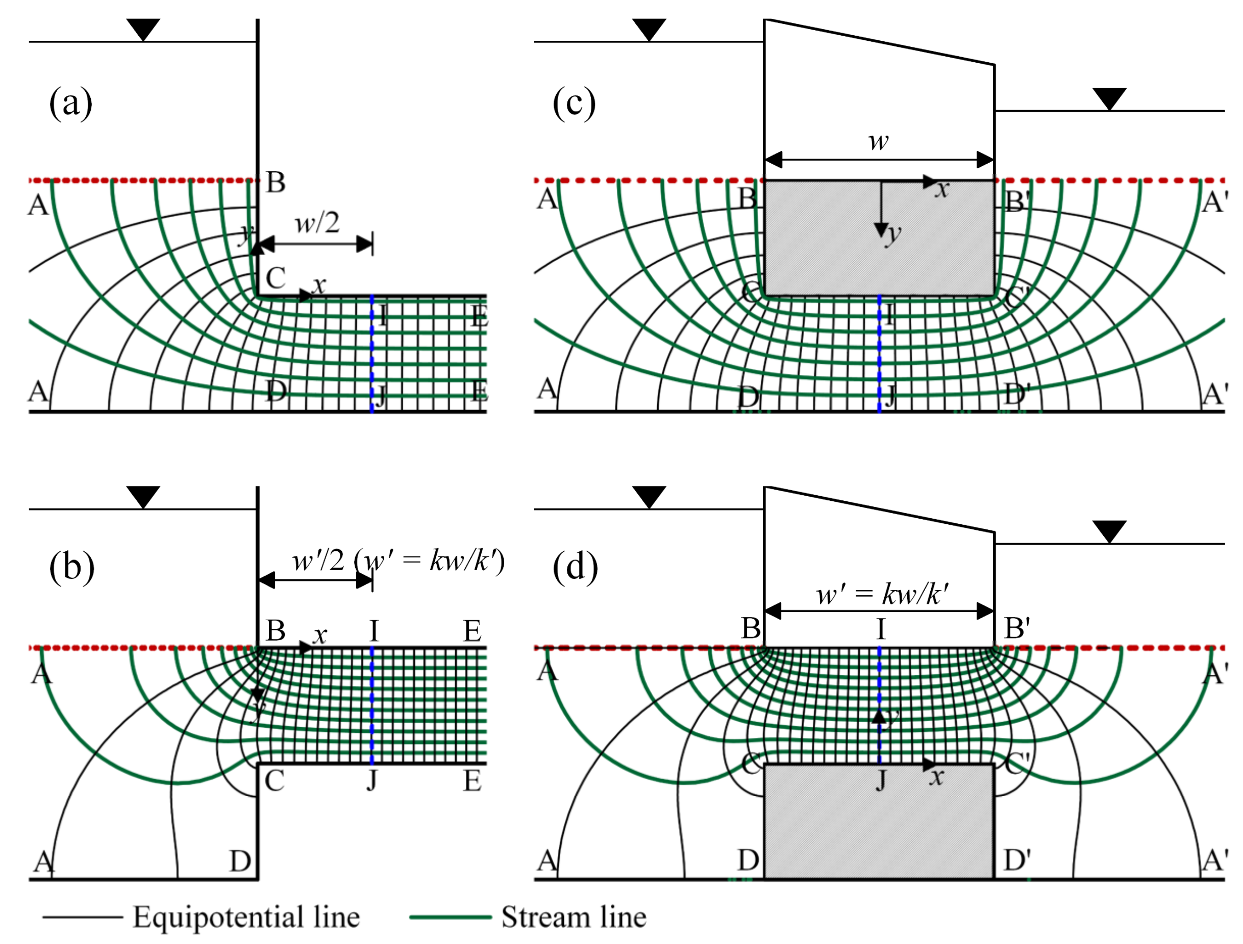
The models in
Figure 2a,c have exact solutions. The former can be derived from the analytical solution of Wang [
26], and the latter can be derived by performing the Schwarz–Christoffel transformation (SCT) [
32]. The normalized average drawdowns can be obtained from these two analytical solutions. However, these two analytical solutions involve Legendre’s elliptic integrals of the first and third kinds, which means the normalized average drawdowns cannot be expressed explicitly but must be solved numerically. To facilitate the engineering application, the models in
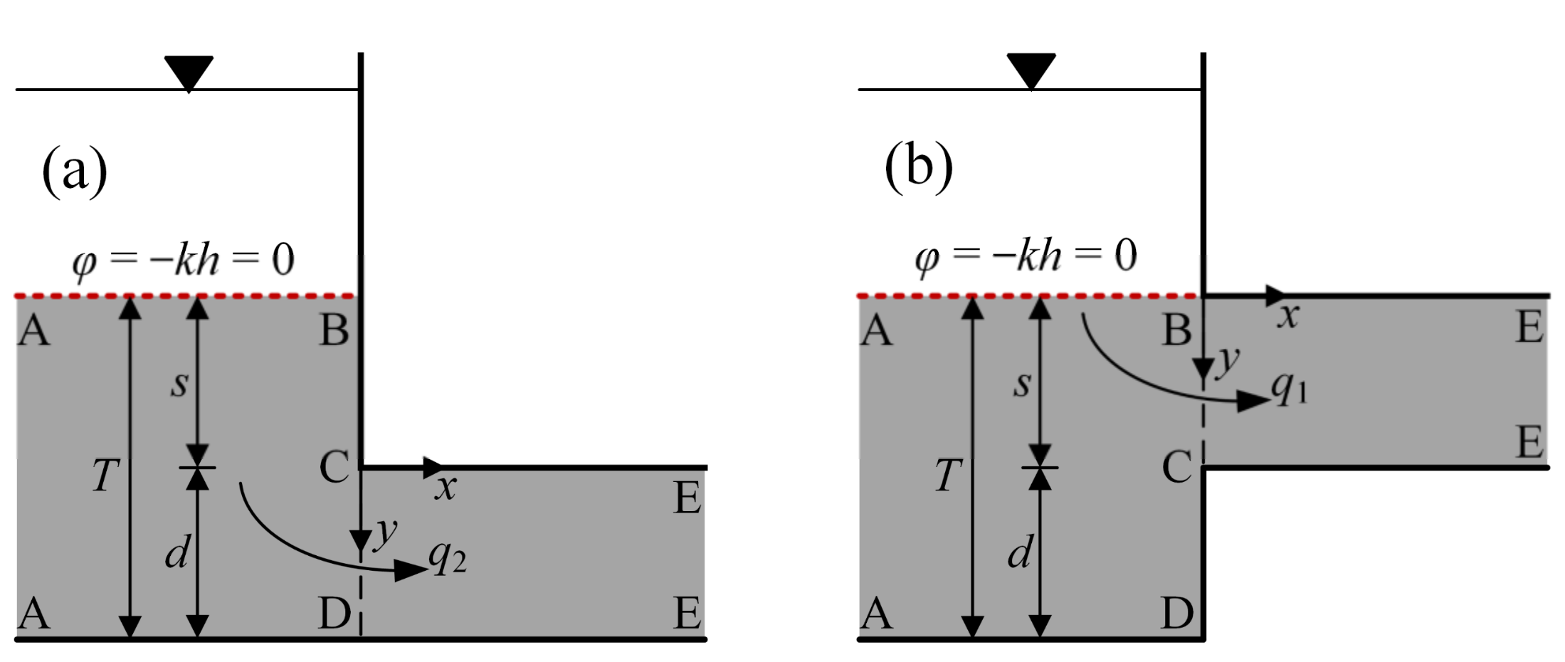
Figure 2a,c are further simplified to two approximate models, as described in
Figure 3a and
Figure 3b, respectively, assuming that the ratios
w/
d and
w’/
s are sufficiently large. The two approximate models are used to derive the approximate solutions of the normalized average drawdowns. The exact solutions are used to check and correct the approximate solutions, thereby obtaining the approximate expressions of the normalized average drawdowns.
2.2.1. Analytical Solutions for the Approximate Models
The analytical solution for the model in
Figure 3a can be obtained from the study of Aravin and Numerov [
23]. As described in
Figure 3a, the origin is at the point C, and the head value along the pervious boundary AB is assumed to be zero. From the study of Aravin and Numerov [
23], the relationship between the complex physical plane (
z =
x +
iy) and the complex potential plane (
ω =
φ +
iψ) is as follows:
where
h0 is the head value at point C, which is expressed as
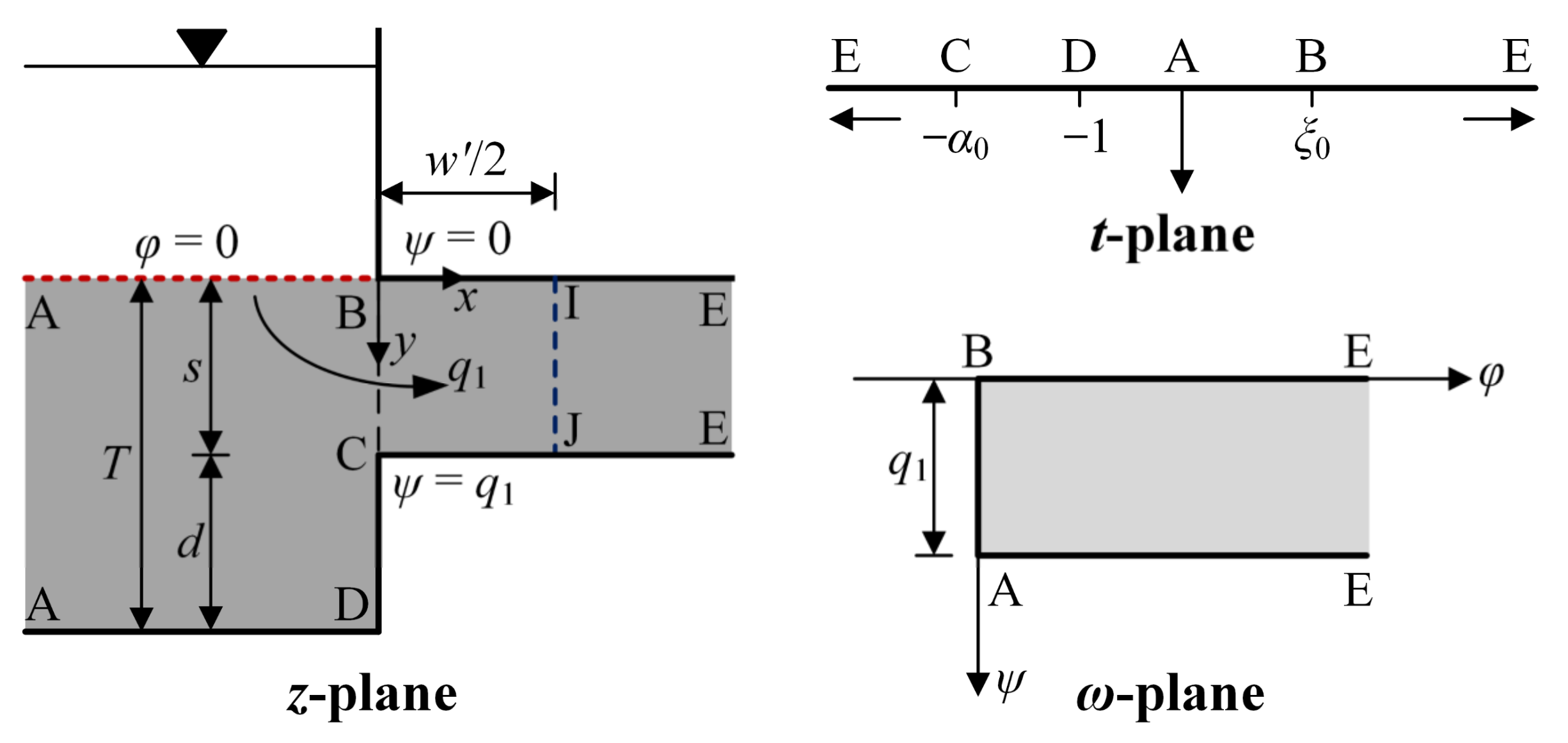
The analytical solution for the model in
Figure 3b can be derived by performing the Schwarz–Christoffel transformation [
34]; the mapping is described in
Figure 4. The
t-plane is used as an auxiliary plane, and the
z-plane and
ω-plane are mapped to the lower part of the
t-plane.
As described in
Figure 3b, the origin is at point B, and the head value along the pervious boundary AB is assumed to be zero. Finally, the relationship between the complex physical plane (
z =
x +
iy) and the complex potential plane (
ω =
φ +
iψ) is given as follows:
where
t is an auxiliary variable;
ξ0 is determined by
From the above two analytical solutions, the head value and stream function at each point can be obtained for the models in
Figure 3a,b, and hence calculated flow nets are drawn in
Figure 5a and
Figure 5b, respectively. When the ratios
w/
d and
w’/
s are sufficiently large, using the analytical solutions for the exact models in
Figure 2a,c, calculated flow nets are drawn in
Figure 5c and
Figure 5d, respectively. For the calculated examples in
Figure 5a,c, the head value along the segment AB is identical, and the flow rate
q2 is also identical. In
Figure 5b,d, the head value along the segment AB is identical, and the flow rate
q1 is also identical.
As shown in
Figure 5c, the equipotential line at the location IJ (along the axis of symmetry) is a vertical line. From
Figure 5a, the equipotential line at the location IJ (
x =
w/2) is close to a vertical line. Theoretically, if this equipotential line is vertical, both the boundaries and flow net in the region ABCIJDA in
Figure 5a are the same as those in
Figure 5c. Hence, when
w/
d is sufficiently large, the normalized average drawdowns on the segments BC and CD in
Figure 2a can be equivalent to those in
Figure 3a.
Similarly, when the ratio
w’/
s is sufficiently large, the normalized average drawdowns on the segments BC and CD in
Figure 2c can be equivalent to those in
Figure 3b. As shown in
Figure 5b,d, the regions ABIJCDA have the same boundaries and flow nets, for the equipotential line at the location IJ (
x =
w’/2) in
Figure 5b is close to a vertical line.
2.2.2. Approximate Expressions for RBC(q2) and RCD(q2)
From
Figure 5a, if
x is sufficiently large, the equipotential lines are vertical, and hence the head value has nothing to do with
y, but only with
x. From the study of Aravin and Numerov [
23], the asymptotic equation of the head value
h(
x) when
x is sufficiently large is expressed as
In the region ECDE in
Figure 3a, the segments CE and DE are impervious boundaries, and the vertical hydraulic gradient along the segments is zero. Hence, the average head
(
x) at any
x–location (
x ≥ 0) within this region is a linear function, which can be expressed as
where
CD(q2) is the average head on the segment CD in
Figure 3a.
When
x is sufficiently large, the relationship
(
x) =
h(
x) is obtained. Substituting Equations (14) and (16) into
(
x) =
h(
x) gives
CD(q2) = −
q2/
k·
R1. Then, considering that the upstream head in
Figure 3a is zero, the normalized average drawdown on the segment CD is expressed as
The conditions on the segment BC are
z =
iy (−
s ≤
y ≤ 0) and
ω = −
kh. Substituting them into Equation (7), the head value on the segment BC is obtained:
Then, the normalized average drawdown on the segment BC is expressed as
where the
kh/
q2 value is determined by Equation (18).
2.2.3. Approximate Expressions for RBC(q1) and RCD(q1)
From
Figure 5b, if
x is sufficiently large, the equipotential lines are vertical, and the head value has nothing to do with
y but only with
x. When
x → ∞,
h → −∞ and
φ = −
kh → ∞ can be obtained. Substituting
φ → ∞ into Equation (11) gives
t → ∞. Then, substituting
t → ∞ into Equation (10) gives
t’ → 1. Finally, substituting
t’ → 1 into Equation (9), the asymptotic equation of the head
h(
x) is expressed as
In the region EBCE in
Figure 3b, the segments BE and CE are impervious boundaries, and hence the average head
(
x) at any
x–location (
x ≥ 0) within this region is a linear function, which can be expressed as
where
BC(q1) is the average head on the segment BC in
Figure 3b.
When
x is sufficiently large, the relationship
(
x) =
h(
x) is obtained. Substituting Equations (20) and (22) into
(
x) =
h(
x) gives
BC(q1) = −
q1/
k·
R2. Then, considering that the upstream head in
Figure 3b is zero, the normalized average drawdown on the segment BC is expressed as
The conditions on the segment CD are
z =
iy (
s ≤
y ≤
T) and
ω = −
kh +
iq1. Substituting them into Equations (9) and (11), the head value on the segment CD is obtained:
when
y =
s,
kh/
q1 = (−2/π)sinh
−1[
T/(
s)]; when
y =
T,
kh/
q1 = (−2/π)sinh
−1[1/
].
Then, the normalized average drawdown on the segment CD is expressed as
where the
kh/
q1 value is determined by Equations (24) and (25).
2.2.4. Correction
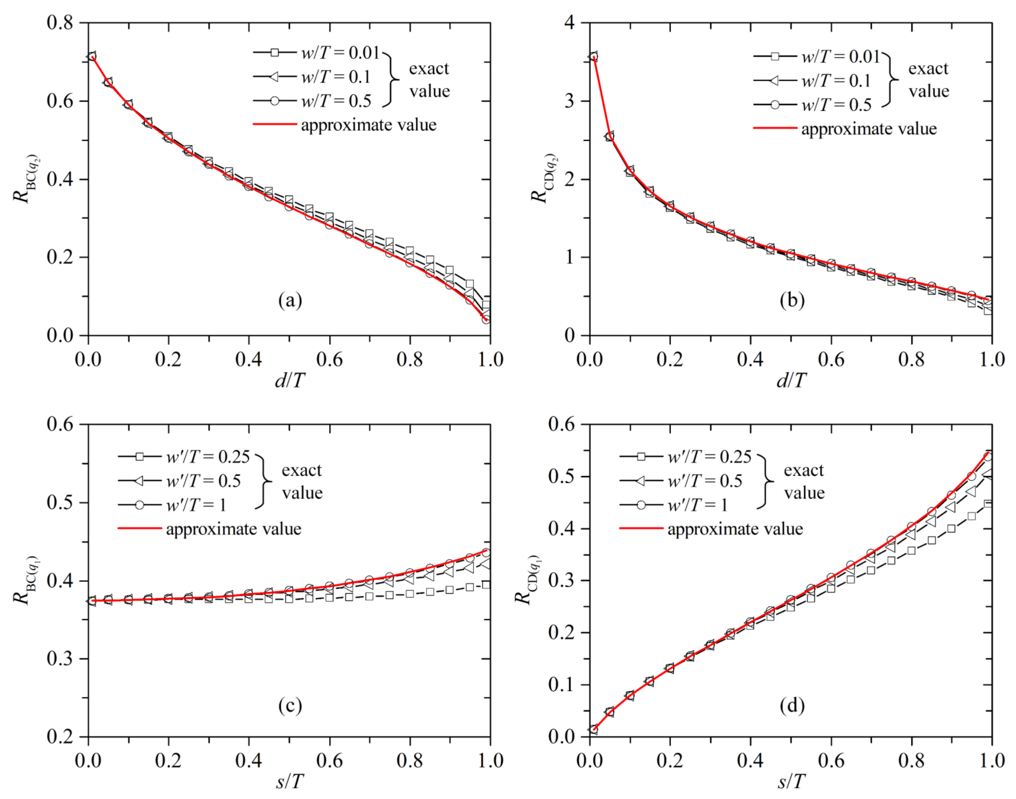
The exact and approximate solutions are used to calculate the four normalized average drawdowns, respectively.
Figure 6a–d present the calculation results of
RBC(q2),
RCD(q2),
RBC(q1), and
RCD(q1), respectively.
From
Figure 6, the approximate values have nothing to do with
w/
T and
w’/
T but only with
s/
T (or
d/
T). The exact values change with
w/
T or
w’/
T, and their curves gradually converge to the curves of the approximate values.
From
Figure 6a,b, with an increase in
w/
T or a decrease in
d/
T, either of which leads to an increase in
w/
d, the approximate values are closer to the exact values. For
RBC(q2), the approximate values are very close to the exact values when
w/
T > 0.1 or
d/
T < 0.5. For
RCD(q2), the approximate values are close to the exact values on the whole; only when
d/
T ≥ 0.9 and
w/
T < 0.5 do the results show a large deviation between the approximate and the exact values.
From
Figure 6c,d, with an increase in
w’/
T or a decrease in
s/
T, either of which leads to an increase in
w’/
s, the approximate values are closer to the exact values. The approximate values are very close to the exact values when
w’/
T > 0.5 or
s/
T < 2
w’/
T. The ratio
w’/
T > 0.5 is easy to achieve in engineering practice.
By contrast, when w/d or w’/s is small, the deviation between the approximate and exact values is large. In this case, it may cause a certain error in the seepage calculation if the approximate solutions are directly used to calculate the normalized average drawdowns. Therefore, the correction for the approximate solutions is needed.
Figure 7 presents the calculation results of the normalized flow rate
q/(
kH), based on Equation (6). Here,
s/
T = 0.1 and
k’/
k = 0.1 are adopted for
Figure 7a;
s/
T = 0.75 and
k’/
k = 0.9 are adopted for
Figure 7b. The four normalized average drawdowns in Case 1 are all calculated by the exact solutions. In addition, in Cases 2–5, three normalized average drawdowns are calculated by the exact solutions, whereas the fourth is calculated by the approximate solutions. In Cases 2–5,
RBC(q2),
RCD(q2),
RCD(q1), and
RBC(q1) are calculated by the approximate solutions, respectively. Then, the flow calculation results in Cases 2–5 are compared with those in Case 1, respectively, and the effects of the approximate values of the four normalized average drawdowns on the flow calculation results are studied.
From
Figure 7, the calculation results in Cases 2 and 4 are close to those in Case 1, whereas the results in Cases 3 and 5 differ from those in Case 1. The results show that using the approximate values of
RBC(q2) and
RCD(q1) does not affect the calculation results. However, the approximate values of
RCD(q2) and
RBC(q1) exerts a notable effect on the calculation results.
To sum up, RBC(q2) and RCD(q1) can be directly calculated by the approximate solutions, regardless of the value of w/d and w’/s. To avoid large errors in the flow calculation results, approximate solutions for RCD(q2) and RBC(q1) need to be corrected within the following scopes: s/T ≤ 0.1(or d/T ≥ 0.9) and w/T < 0.5 (for RCD(q2)); w’/T ≤ 0. 5 and s/T ≥ 2w’/T (for RBC(q1)). Outside the scopes, the approximate solutions can be directly used to calculate RCD(q2) and RBC(q1).
The ratio of exact and approximate values of the normalized average drawdowns is used as the correction coefficient. Within the scopes of correction,
RCD(q2) and
RBC(q1) are the product of the approximate values and the correction coefficients. Data fitting is applied to obtain the correction coefficients suitable for the scopes of correction:
where
β1 and
β2 are the correction coefficients for
RCD(q2) and
RBC(q1), respectively.
Based on Equations (17) and (23), the approximate expressions for calculating
RCD(q2) and
RBC(q1) are
Although the approximate solutions can be directly used to determine
RBC(q2) and
RCD(q1), the integrals of Equations (19) and (26) need to be solved numerically. The numerical integration scheme seems unattractive to engineers. To facilitate the calculation, linear fitting is adopted to obtain the simplified formulas for
RBC(q2) and
RCD(q1).
Figure 8a,b present the fitting results for
RBC(q2) and
RCD(q1), respectively. The fitting curves have large correlation coefficients and satisfactory accuracy. Finally, the approximate expressions for
RBC(q2) and
RCD(q1) are
2.3. Implementation
Based on the approximate expressions (29)–(32), the four normalized average drawdowns RBC(q2), RCD(q2), RBC(q1), and RCD(q1) can be determined by simple calculation. Then, substituting them into Equations (5) and (6), the flow rates q1, q2, and q are obtained.
Substitute the calculated
q1 and
q2 into the exact models in
Figure 2a,c, and use the analytical solutions of the two models to obtain the drawdowns in the regions ABCDA and A’B’C’D’A’. Then, by the superposition of the drawdowns of the two models, the drawdowns at each point in
Figure 1c can be obtained. Finally, the head value at each point is the difference between the upstream or downstream head and the obtained drawdowns. When
w/
d and
w’/
s are sufficiently large, the approximate models in
Figure 3a,b can be used to replace the two exact models to determine drawdowns at each point.
In engineering practice, people pay more attention to the quantity of seepage. The quantity of seepage (or flow rate) in the aquitard (including leakage through the wall body and seepage under the wall) can be quickly estimated by Equations (5) and (6). The following sections focus on the flow calculation.
3. Verification and Discussion
For general cases, the accuracy and applicability of the proposed method (TPM) are verified compared with the numerical method.
The proposed method contains solutions for the following four special cases:
The wall penetration depth in the aquitard is zero (s/T = 0).
The cut-off wall fully penetrates the aquitard (s/T = 1).
The wall permeability is very small compared to the aquitard permeability.
The wall thickness is very small compared to the aquitard thickness.
There have been several analytical solutions for these four special cases. They can be obtained from the studies of Aravin and Numerov [
23], Anderson [
31], Wang [
26], and Yakimov and Kacimov [
32], respectively. For convenience, these analytical solutions are denoted as Aravin, Anderson, Wang, and Yakimov, respectively.
Here, the proposed method is compared with these analytical solutions to verify that it is also applicable to these special cases. For general cases where these analytical solutions are not applicable, the proposed method is also applicable, which can be proved by the comparison with the numerical method. In addition, the effects of the wall permeability and thickness on the flow rate are discussed compared with Wang and Yakimov, respectively.
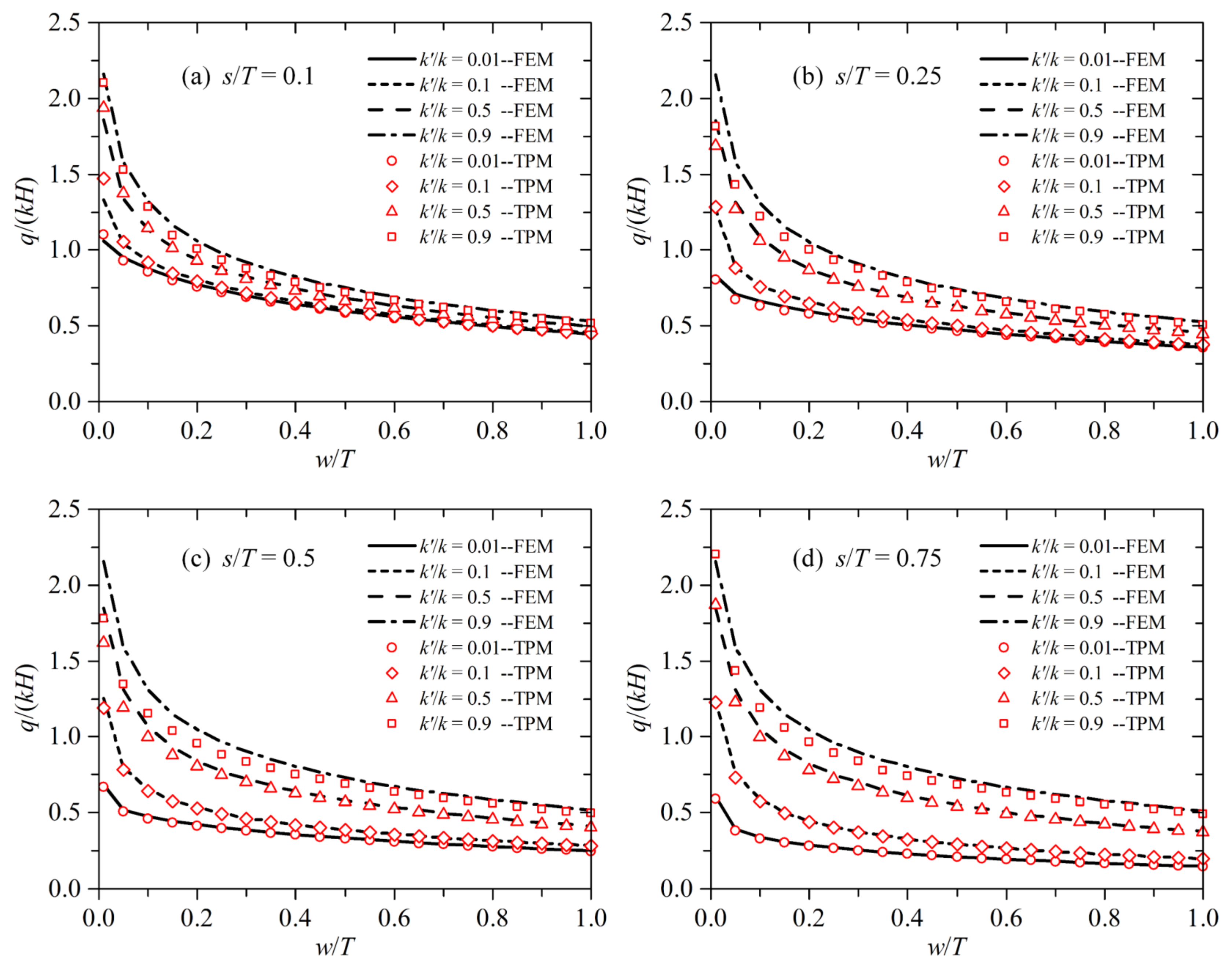
3.1. Comparison with the Numerical Method in General Cases
The professional finite element software ABAQUS (Version 6.14-4) is used as a tool of the numerical method. To avoid the flow calculation results from being affected by the boundaries AA and A’A’, the horizontal length of the aquitard on one side of the cut-off wall is recommended to be more than three times the aquitard thickness. The numerical model obeys the boundary conditions in
Figure 1c described earlier.
Representative examples are verified by the comparison between the proposed method (TPM) and the finite element method (FEM). The following parameters are adopted:
k’/
k = 0.01, 0.1, 0.5, 0.9;
s/
T = 0.1, 0.25, 0.5, 0.75;
w/
T = 0.01–1. The flow calculation results of the examples for
s/
T = 0.1, 0.25, 0.5, 0.75 are presented in
Figure 9a–d, respectively.
From
Figure 9, the results of TPM are in good agreement with those of FEM when
k’/
k ≤ 0.5. When
k’/
k > 0.5, a deviation between the results of TPM and FEM occurs. The deviation increases as an increase in
k’/
k. Nevertheless, the deviation decreases as an increase in
w/
T. In addition, the deviation first increases as an increase in
s/
T and then decreases as an increase in
s/
T.
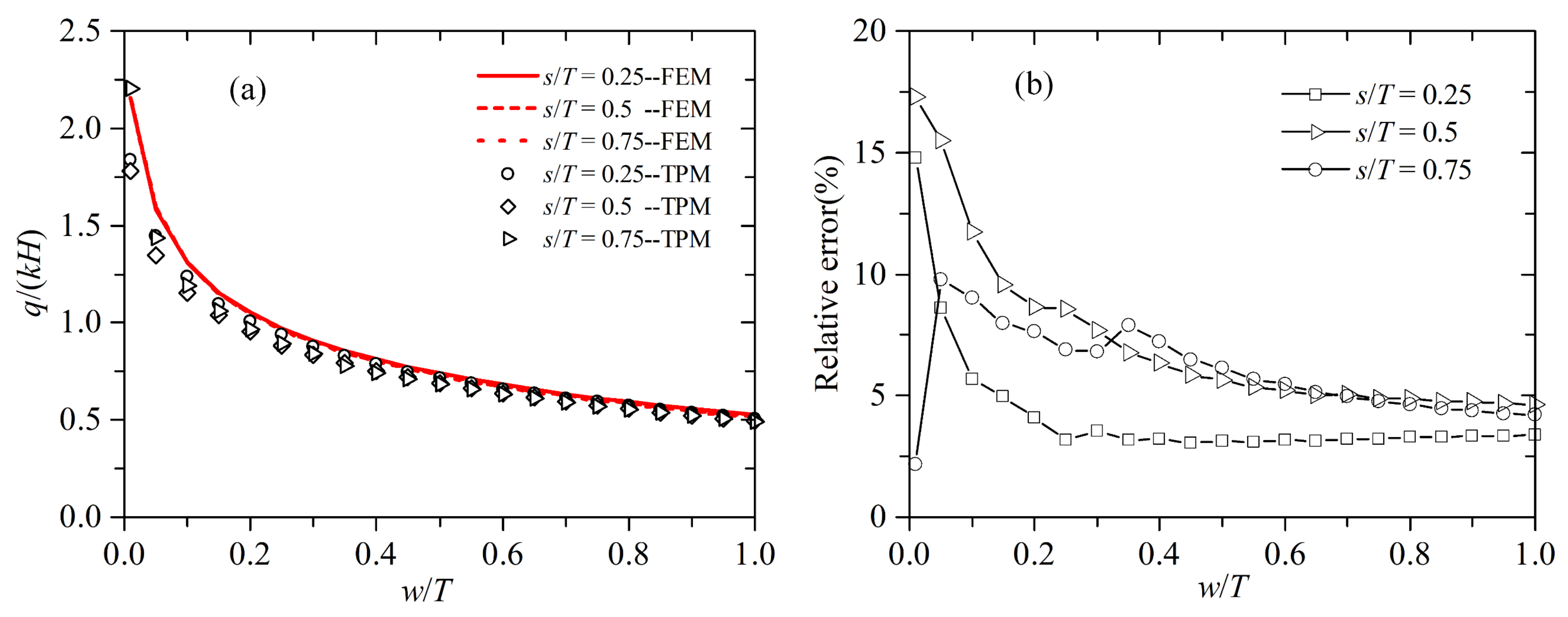
To find the potential maximum deviation,
Figure 10a shows the flow calculation results of TPM and FEM when
k’/
k = 0.9. The ratio
k’/
k = 0.9 is adopted here, because the change in flow rate is very small as an increase in
k’/
k when 0.9 ≤
k’/
k < 1. From
Figure 10 a, the result curves of FEM coincide when
s/
T = 0.25, 0.5, and 0.75, indicating that the ratio
s/
T has little effect on the flow rate. The relative error of the results between TPM and FEM is calculated, whose formula is |
qTPM −
qFEM|/
qFEM × 100(%). The
qTPM and
qFEM represent the flow calculation results of TPM and FEM, respectively.
The relative error is shown in
Figure 10 b. It can be seen that the potential maximum deviation occurs when
w/
T is small, and it is less than 20%. When
w/
T > 0.1, the relative error is less than 10%. Thus, when 0.5 <
k’/
k < 1, the proposed method can be considered satisfactory in the accuracy and applicability.
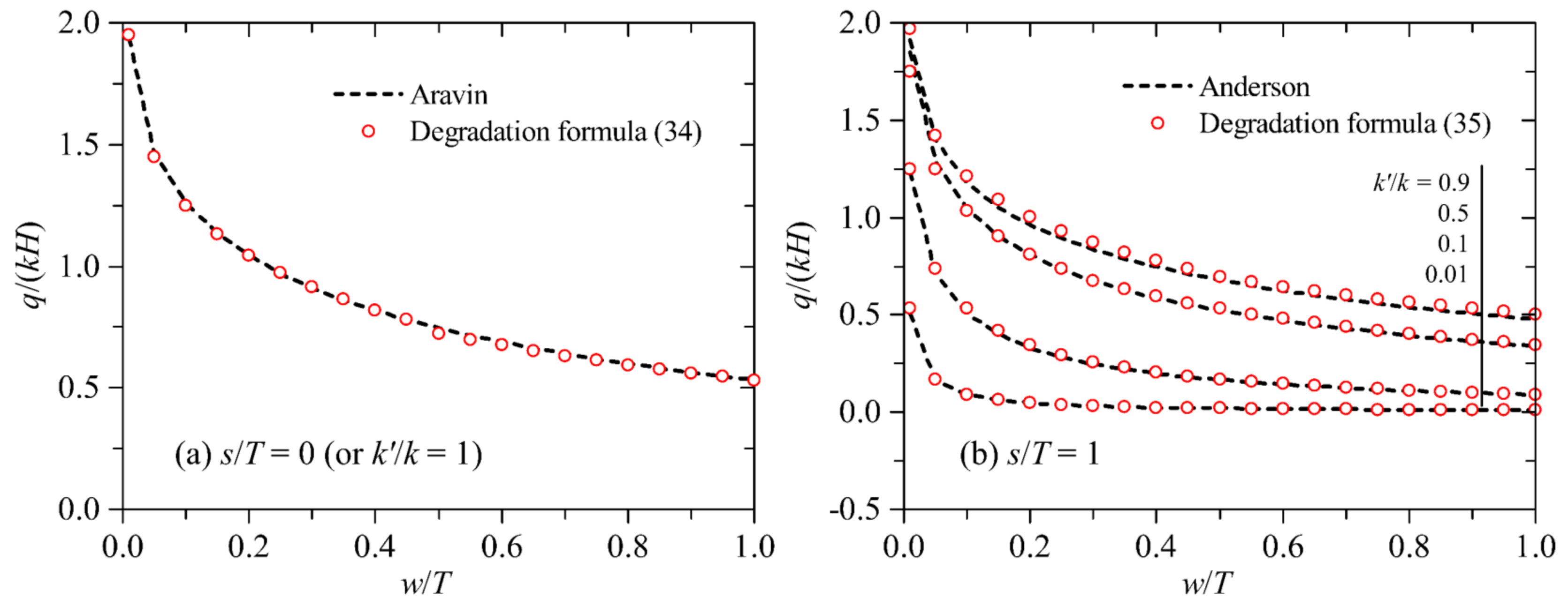
3.2. Special Cases where the Ratio s/T Is Zero or One
When the wall penetration depth in the aquitard is zero, seepage only occurs under the wall; when the cut-off wall fully penetrates the aquitard, seepage only occurs through the wall body. For these two special cases, the proposed method in this study can be degenerated into models that do not need superposition of drawdowns. Rewrite the flow calculation Formulas (5) and (6) into the degradation formulas suitable for the special cases of
s/
T = 0 (or
k’/
k = 1) and
s/
T = 1, as shown in Equations (33) and (34), respectively. When
k’/
k = 1, the flow rate is not affected by
s/
T, and hence this case is equivalent to the case of
s/
T = 0.
When
s/
T = 0 (or
k’/
k = 1), the degradation Formula (33) is compared with Aravin, and the flow calculation results are shown in
Figure 11a. When
s/
T = 1, the degradation formula (34) is compared with Anderson, and the flow calculation results are shown in
Figure 11b. From
Figure 11, the results of the degradation formulas are in good agreement with those of the two analytical solutions, which indicates that the degradation formulas are suitable for the special case of
s/
T = 0 (or
k’/
k = 1) and
s/
T = 1.
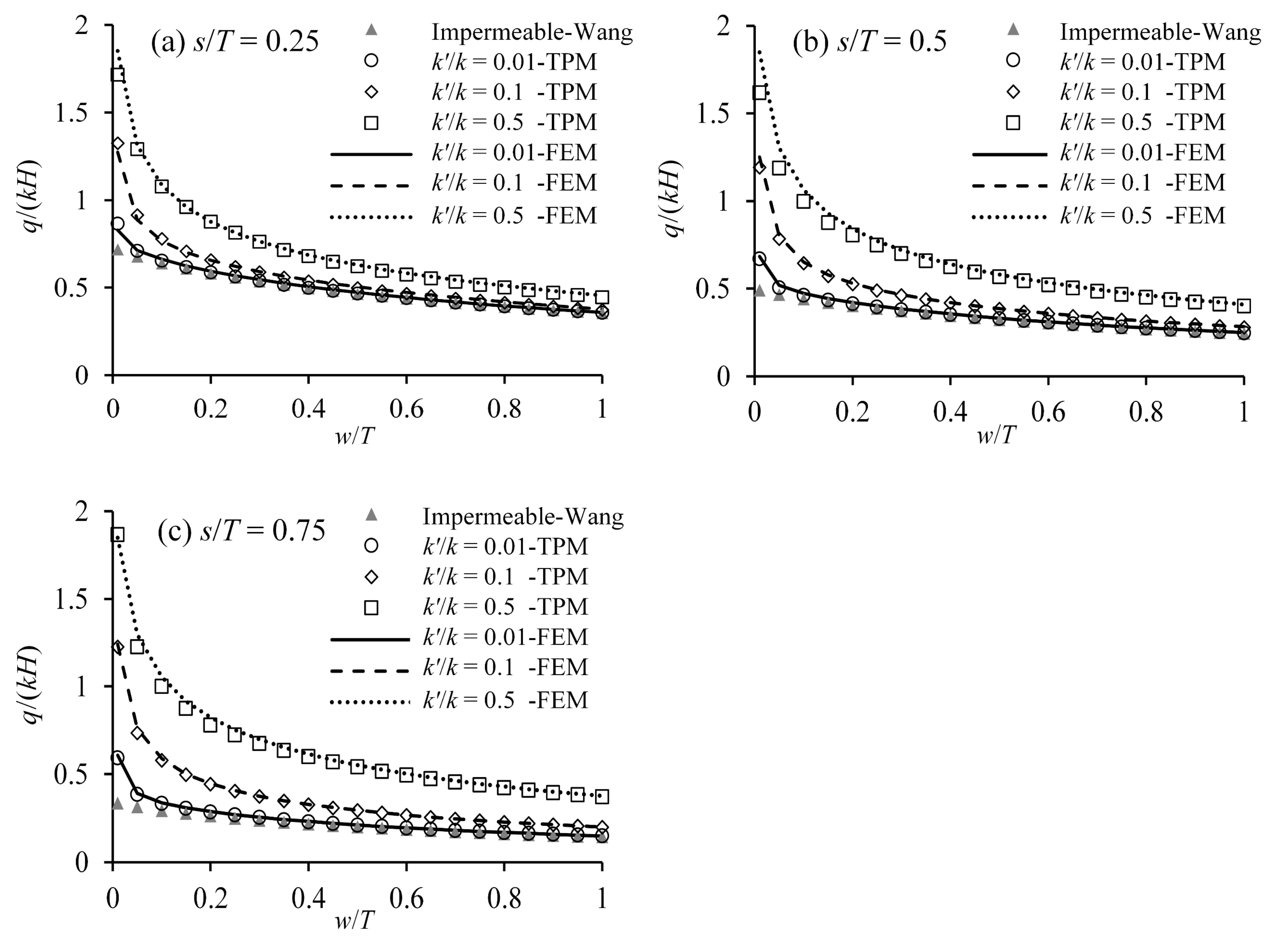
3.3. Effect of Wall Permeability
A comparison of flow calculation results among Wang, TPM, and FEM is shown in
Figure 12.
Figure 12a–c show the results for
s/
T = 0.25, 0.5 and 0.75, respectively.
From
Figure 12, the wall permeability has a big impact on the calculated flow results. When the permeability ratio
k’/
k is very small—that is,
k’/
k = 0.01—the results of TPM and Wang coincide with those of FEM, except for a slight difference where
w/
T is very small. The results show that the wall permeability can be neglected when it is very small compared to the aquitard permeability, and TPM and Wang are both suitable. When the wall permeability is neglected, seepage only occurs under the wall. Then, the model in
Figure 1c can be degenerated into the model in
Figure 2a and the degradation formula for the flow rate is expressed as Equation (33).
When k’/k is large (k’/k > 0.01), the results of TPM are consistent with those of FEM, for the effect of wall permeability has been considered by the TPM method. In this case, the results of Wang differ from those of FEM. The reason is that the quantity of leakage through the wall body increases as an increase in k’/k, whereas the leakage is not considered by Wang. It can also be seen that the difference in the results between Wang and FEM increases as a decrease in w/T or an increase in s/T; in these cases, the quantity of leakage through the wall body has a large proportion in the total flow rate. The difference shows that the effect of the wall permeability on the flow rate should be considered when k’/k > 0.01, especially when w/T is small or s/T is large.
3.4. Effect of Wall Thickness
A comparison of flow calculation results among Yakimov, TPM, and FEM is shown in
Figure 13. The ratio
s/
T = 0.5 and
k’T/(
kw) = 10
−6, 0.001, 0.1, 0.25, 0.5, 1, 2.5, and 5 are adopted here, which makes it easy to obtain the flow calculation results of Yakimov.
Figure 13a–c show the results for
w/
T = 0.01, 0.1, 0.5, and 1, respectively.
From
Figure 13, the wall thickness has a great influence on the calculated flow results. When the thickness ratio
w/
T is very small—that is,
w/
T = 0.01—the calculated results of TPM and Yakimov are very close to those of FEM. The results indicate that the wall thickness can be neglected when it is very small compared to the aquitard thickness, and TPM and Yakimov are both suitable.
While w/T is large (w/T > 0.01), the calculated results of TPM are consistent with those of FEM, for the effect of wall thickness has been considered by the TPM method. In this case, the results of Yakimov differ from those of FEM, as the assumption w/T → 0 was applied to obtain the solution. Furthermore, the difference in the results of Yakimov and FEM increases as an increase in w/T. The difference indicates that the effect of the wall thickness should be considered when w/T > 0.01.


