
Deformation Prediction of Cihaxia Landslide Using InSAR and Deep Learning

1
State Key Laboratory of Eco-Hydraulics in Northwest Arid Region, Xi’an University of Technology, Xi’an 710048, China
2
Tianjin Port Engineering Institute Ltd. of CCCC First Harbor Engineering Company Ltd., Tianjin 300222, China
*
Author to whom correspondence should be addressed.
Water 2022, 14(24), 3990; https://doi.org/10.3390/w14243990
Submission received: 23 September 2022
/
Revised: 12 November 2022
/
Accepted: 15 November 2022
/
Published: 7 December 2022
(This article belongs to the Special Issue Safety Monitoring and Management of Reservoir and Dams)
Abstract
:Slope deformation monitoring and analysis are significant in the geological survey of hydraulic engineering. However, predicting future slope deformation is a vital and challenging task for engineers. The accurate estimation of slope displacement is required for the risk assessment of slope stability. This study was conducted using slope deformation data obtained by interferometric synthetic aperture radar. Five typical points of the slope in different zones were selected to establish the prediction model. Based on the observed data, a prediction model based on long short-term memory (LSTM) and autoregressive integrated moving average (ARIMA) was proposed. Firstly, ARIMA and LSTM models were used separately to predict slope deformation. Root mean square error, mean absolute error, and R2 were used to evaluate the performance of the models, and the results showed that LSTM is more effective than ARIMA. It denotes that the LSTM model can catch the trend in the data sequence with time, and ARIMA is good at predicting the bias in the stationary data sequence. Then, the predictions of ARIMA were added to the original data while the new data were fed to the LSTM model. For most data points, our LSTM-ARIMA model achieved good performance, indicating that the model is robust in slope deformation prediction. The effectiveness of the proposed LSTM-ARIMA model will enable engineers to take corresponding measures to prevent accidents before landslides occur.
1. Introduction
Landslides are a significant disaster in hydraulic engineering projects, which not only constitute a considerable threat to engineering management but also destroy the environment. In China, landslides occur frequently and cause mass casualties and property damage yearly. As complex geological conditions and a harsh construction environment typically surround hydraulic engineering projects, engineers struggle to escape and save injured rescuers in the event of a landslide. Therefore, the study of landslide mechanisms and slope deformation is significant, as it can help to develop proactive measures for landslide prevention.
Some scholars’ studies have investigated the mechanism behind rock slope deformation. Zhang et al. [1] studied the toppling mechanisms and used numerical methods to simulate the deformation mechanism, considering the geological survey, adit prospecting, borehole logging, and sonic test data. The results showed that the method was appropriate for toppling evolution analysis. Zhang et al. [2] also studied the toppling failure mode of a slope under the influence of an earthquake using the discrete element numerical method. Yan et al. [3] proposed a comprehensive control measure, i.e., “drainage + unloading + support”, noting that drainage should be addressed to prevent landslides in Jinjiling. In the research on slope deformation and landslide mechanisms, scholars have analyzed the influence of rainfall [4,5,6], groundwater [7,8,9], and rock compositions [10,11,12]. However, established models are typically only effective for specific engineering projects and thus poor in generalization ability. The complexity of landslide and slope deformation mechanisms hinders the development of a generic model.
It has been argued that an accurate observation is significant in slope deformation analysis. Hence, multiple types of sensors are adopted in slope monitoring in real engineering projects. Optical fiber sensors (OFS) [13,14] are widely used for monitoring slope deformation. Distributed optical sensors [15] are highly effective for monitoring the deformation to evaluate the potential for landslide occurrence. Other common techniques for landslide analysis are the observation of slope deformation, high-resolution imaging, and computer vision. Parente et al. [16] used at least four digital single-lens reflex cameras to build a monitoring system and estimate image differences through three-dimensional scene reconstruction. Li et al. [17] used unmanned aerial vehicles and the U-Net model to monitor landslide deformation. This technique is new and has only been verified in several engineering projects. An accurate monitoring technique is terrestrial laser scanning: Li et al. [18] used terrestrial laser scanning point clouds to obtain slope geometric information and assess slope deformation quantitatively. Li et al. [19] used terrestrial laser scanning techniques to observe rock movement on a high slope, and the results showed that the method was effective. However, terrestrial laser scanning is expensive and unsuitable for large-scale slope monitoring. Therefore, the interferometric synthetic aperture radar (InSAR) technique has been proposed for monitoring slope deformation. Sun et al. [20] examined the deformation of a slope for approximately three years prior to the landslide using 16 ascending InSAR images. Dai et al. [21] used InSAR to recognize the potential landslides in Gansu Province. Zhang et al. [22] used InSAR to investigate slowly developed landslides of a mountain with steep topography. Conducting slope deformation using the InSAR technique is inconvenient and depends on the engineers’ experience.
In terms of analyzing the monitoring data of slope deformation, the use of statistical models has been proposed. Tang et al. [23] compared logistic regression, the weight of evidence, and information value models to assess different types of landslides considering causal factors. Li and Huang [24] proposed a kernel grey model considering a fractional operator to predict landslide displacement. Shahabi et al. [25] applied frequency ratio, logistic regression, and fuzzy logic to conduct susceptibility mapping using remote sensing data. The working of statistical models can be explained, but they perform worse than machine learning algorithms.
Machine learning algorithms are widely applied to slope deformation monitoring data in predicting slope deformation, and the algorithms include support vector machine (SVM) [26,27,28], random forest (RF) [29,30], and artificial neural networks (ANN) [31,32,33]. Optimized and improved models based on intelligent algorithms have been established for specific data sequences. Zhang et al. [34] proposed an ensemble model (RF model with Bayesian optimization and the Kalman filter) to predict slope deformation monitoring data trends for cumulative slope displacement. Deng et al. [35] used an extreme learning machine optimized with the lasso algorithm to predict landslide displacement trends. Garg et al. [36] used ARIMA to analyze long-term noise monitoring data and found that the ARIMA approach is reliable for time-series modeling of traffic noise levels. Hu et al. [37] used a combined LSTM–ARIMA model to predict dam deformation and found that the ARIMA model is suitable for processing complex nonstationary time series data.
Deep learning models that consider time series data features have also been applied to predicting slope deformation, including recurrent neural network (RNN), gated recurrent unit (GRU), and long short-term memory (LSTM). Chen et al. [38] applied a genetic algorithm-optimized RNN to predict a landslide. The performance of the improved RNN was better than that of the ANN model. Zhang et al. [39] compared multiple intelligent algorithms, including ANN, RF multivariate adaptive regression splines (MARS), and GRU. GRU can identify the local and global information of the data sequence. Yang et al. [40] applied LSTM to analyze landslide displacement and found that the LSTM model can extract the dynamic features of landslides compared with other models. Wang et al. [41] used the CEEMDAN and the attention mechanism combined with the LSTM to establish a dynamic prediction model for landslide displacement. A comparison of results obtained showed that the CEEMDAN-AMLSTM model achieved competitive accuracy. Jiang et al. [42] combined LSTM neural networks and the support vector regression algorithm with optimal weight to predict slope deformation. The proposed ensemble model effectively constructed the mapping relationship between landslide deformation and causative factors. Xing et al. [43] established double moving average decomposition and LSTM network coupling prediction model for landslide displacement. Zhang et al. [44] used LSTM to establish a prediction model, which has a strong advantage for step landslide deformation with short-term impact. These studies show that LSTM is suitable for predicting landslide deformation.
In this study, we propose an LSTM-ARIMA model to predict slope deformation using InSAR data. Typical points of different zones were selected to analyze the slope deformation trend. The ARIMA and LSTM models were first applied individually, and the LSTM model outperformed the ARIMA model. Finally, the ARIMA prediction was taken as a new feature to train the LSTM-ARIMA model. The result shows that the proposed model is robust in slope deformation prediction.
2. Methodology
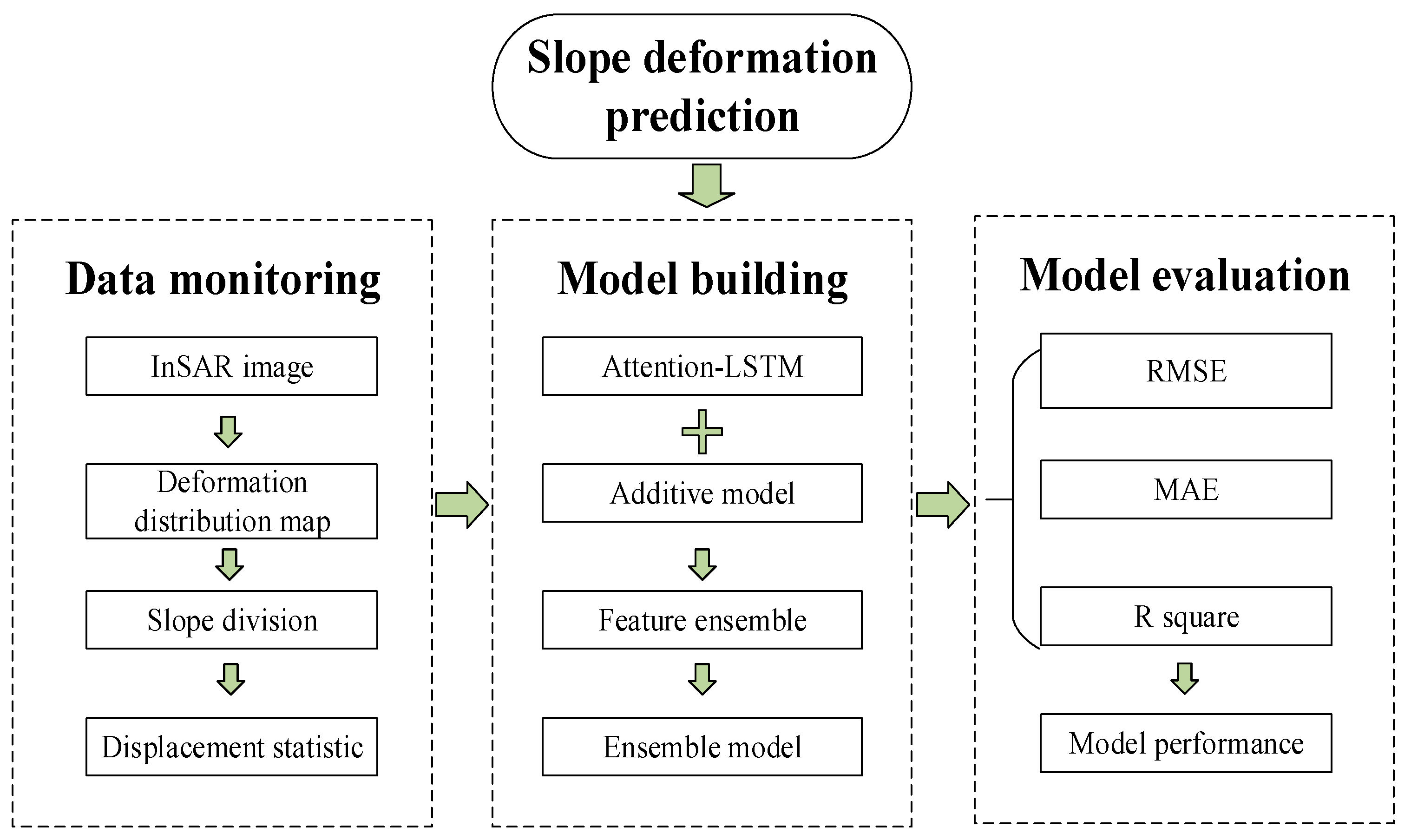
Accurate predictive modeling for slope deformation is significant in engineering construction, especially in hydraulic engineering. Different types of monitoring tools are generally used for observing slope deformation. However, monitoring all parts of a slope and the slope evaluation are difficult. Hence, we propose a slope deformation data analysis and evaluation method based on the InSAR monitoring technique. The research framework is illustrated in Figure 1.
- Data monitoring is the first step in slope deformation prediction. In this study, we used InSAR to acquire slope deformation data. According to the difference between the two observations, the slope deformation distribution map at different periods can be obtained. We divided the target slope into different zones. In the divided zones, we selected a reference point, and the data of the point were used to represent the deformation of the monitored zone. Thus, the curve of the deformation with time was obtained.
- Model building is the second step in slope deformation prediction. In our research, long short-term memory (LSTM) was adopted in deformation prediction. The attention mechanism was also considered in the LSTM establishment. Then, the additive model was used to build training features. Both the original and generated features were fed to the LSTM model. According to the idea of the model ensemble, the final prediction model was established.
- Model evaluation is the final step in slope deformation prediction. To evaluate the slope deformation model, we used three model evaluation metrics, i.e., root mean square error (RMSE), mean absolute error (MAE), and R-square (R2). The model was built using monitored data from five reference points in the 4# landslide of the Cihaxia hydropower station. Finally, the actual data and test results were compared to evaluate the prediction results. Model evaluation is the final step in slope deformation prediction.
We discuss the strengths and weaknesses of slope deformation prediction in this paper. According to our observations, the slope deformation would continue. As the slope deformation may change rapidly or remain stable in the future, the model must be retrained to obtain new rules for the deformation change.
2.1. The Fundamental Principle of InSAR
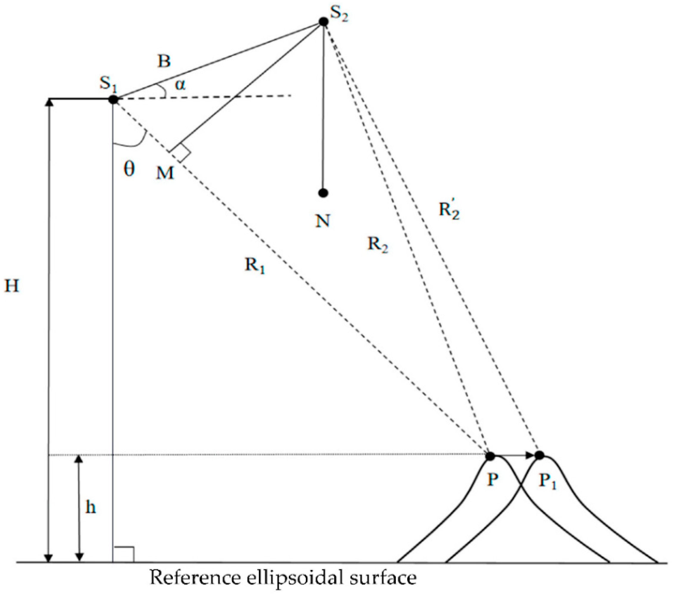
InSAR uses radar technology to acquire two or more SAR images from various observation angles of the same ground area and performs interferometric measurements on the research area. The InSAR technology mainly establishes the correspondence function relationship between phase and surface elevation and surface deformation through phase analysis. The relationship is then used to solve the specific ground elevation and surface shape variables. Figure 2 illustrates the InSAR technical geometry.
As depicted in Figure 2, P is the target ground observation point; S1 and S2 are the antenna positions of the remote sensing platform when the satellite acquires SAR images twice; R1 and R2 are the corresponding slope distances from the satellite to the ground target during the two observations; h is the height from the ground; H is the distance from the satellite to the reference ellipsoid; B represents the spatial baseline between satellite observations; B|| is the component along the radar’s line of sight; B⊥ is the component perpendicular to the radar’s line of sight; Bh is the horizontal projection of baseline B; Bv is the vertical projection of baseline B; α is the angle between the horizontal direction and B; and θ is the radar observer side view. The relationship among all variables is expressed in Equations (1) and (2).
Without considering noise, the radar wave is divided into corresponding absolute phases ψ1 and ψ2 along the slant distances R1 and R2, which can be represented by Equation (3).
where n1 and n2 are phase integers; λ is the wavelength of radar electromagnetic waves; and the non-integer periodic phases of the radar propagation along slant distances R1 and R2 are indicated by ϕ1 and ϕ2, respectively. The length of the reference baseline is much larger than the two slant distances. As shown in the geometric relationship illustrated in Figure 2, both slope distances are parallel to each other. Thus, Equation (4) is obtained as follows:
Substitute the absolute phases ψ1 and ψ2 into Equation (4) to obtain Equation (5).
It can be seen from Equation (5) that factors such as reference ellipsoid surface, ground deformation displacement, and interference geometry can be expressed in the slant distance difference.
During monitoring, if the surface is deformed, the observation point P moves to point P1. The displacement deformation of point P is r, and ∆r is the change in slope distance in the direction of the radar’s line of sight after deformation. After the interferometric processing of the secondary imaging image, the interference phase caused by surface deformation is obtained, as shown in Equation (6).
As the amount of displacement is numerically negligible relative to the slope distances, ; hence, Equation (6) can be expressed as Equation (7).
In Equation (7), the first term on the right-hand side is the combination of the interference phase in the terrain phase and the reference ellipsoidal phase; the second term on the right-hand side is the deformation phase component caused by the surface displacement. The deformation phase φdef can be expressed as Equation (8).
2.2. ARIMA Model
In slope deformation monitoring and analysis, the monitoring data are composed of trends, seasonal items, and bias. In the model establishment, two types of models can be selected: additive model and multiplicative model. The trend, seasonal item, and bias can be expressed as T(t), S(t), and B(t), respectively. The two models are expressed in Equations (9) and (10), respectively.
The multiplicative model can be expressed as:
Equation (11) is also an additive model, denoting that the additive model can reflect the time series features during the model establishment. Hence, the additive model is selected as the slope deformation prediction model.
For a time-dependent series, the inner correlation of the data enables the prediction of the data at a specific time using previous data. The autoregressive (AR) model calculates the predicted value using a linear combination of the sum of previous data and a bias term. The AR model can be expressed as Equation (12).
where and are the true value and the bias, respectively; βi (i = 1,2,3…) are the model parameters. Yt is a linear combination in a moving average (MA) model and can be expressed as Equation (12).
We combine the AR and MA models with the difference method to build the ARIMA model.
αi(i = 1,2,3…) are the model parameters similar to βi.
2.3. LSTM-Attention Model
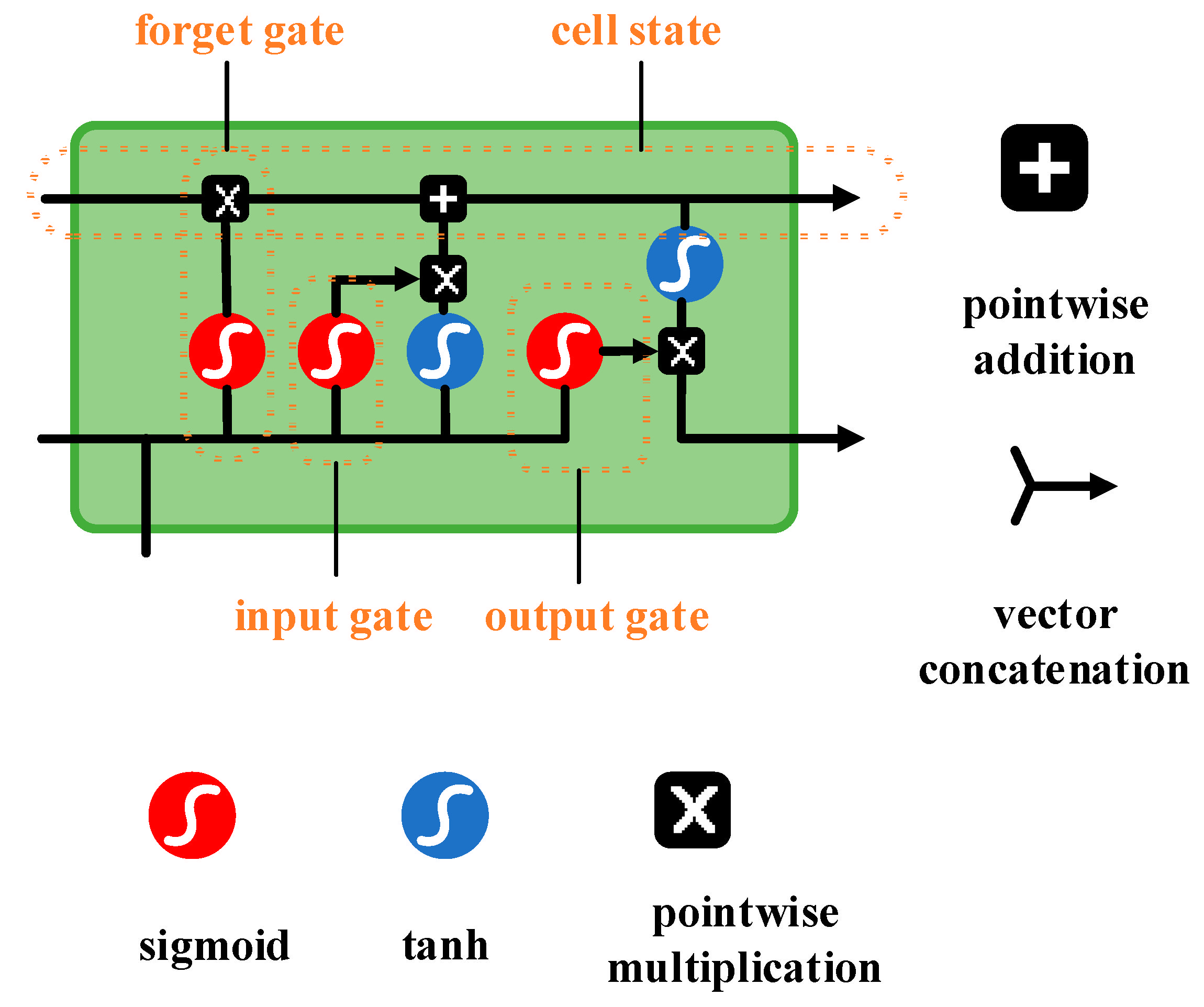
The LSTM is an RNN model with feedback connections. RNN achieves significant performance in time series sequence processing. However, RNN struggles to use information from previous steps in later steps because of its short-term memory. Additionally, the gradient vanishing problem exists in the RNN model; the gradient is a value used to update the weight of the neural network. The gradient vanishing problem occurs when the gradient shrinks as it propagates backward over time. If the gradient becomes extremely small, it contributes little to learning; therefore, the LSTM was proposed. Cells in the LSTM network control learning for a long period. An LSTM cell includes the input gate, output gate, and forget gate, as illustrated in Figure 3. The information transmission is controlled by the three gates in the LSTM block, and the three gates determine the data to keep or discard. The relevant information in the long chain of data sequences can be learned using the gates.
Moreover, the three gates in the LSTM block can be used to solve the gradient vanishing problem. At time t, the gate generates variables it, ft, and ot. Variable ht is the output; ht−1 represents the hidden state and determines how much information is contained from xt to ct. The information transferred to cell state ct−1 is determined by ft, and ot determines the final output, ht. The specific formulae of LSTM are expressed in Equations (14)–(18).
2.4. Attention
The attention mechanism is based on human visual attention, which is attracted by a significant part of a scene while ignoring unnecessary information. This idea is different from that of global attention. The attention mechanism assigns a larger weight to certain parts of a scene as it prioritizes the information of the area of interest in the scene. Therefore, the LSTM model can be optimized by adding an attention mechanism.
In this study, the LSTM model and attention mechanism were combined. As the LSTM model obtains the time series-related information, the attention block selects the critical information in the slope deformation data sequence. In the model training process, the data created by the LSTM are assigned corresponding weights by the attention block, indicating that certain parts of the data are addressed using attention. The attention block can assign corresponding weights automatically in different layers of the LSTM. Equations (19)–(21) express the attention block in the LSTM.
ht is the output of the hidden layers in the LSTM. FA is the output of the attention block, Wt is the weight, and bt is the attention block bias.
2.5. Model Evaluation Metrics
Root mean square error (RMSE), mean absolute error (MAE), and R-square (R2) were selected as the model evaluation metrics to evaluate the model. The metrics are expressed in Equations (22)–(24):
where yi is the prediction, is the actual data, and is the mean of the output data.
3. Case Study
3.1. Engineering Project Review
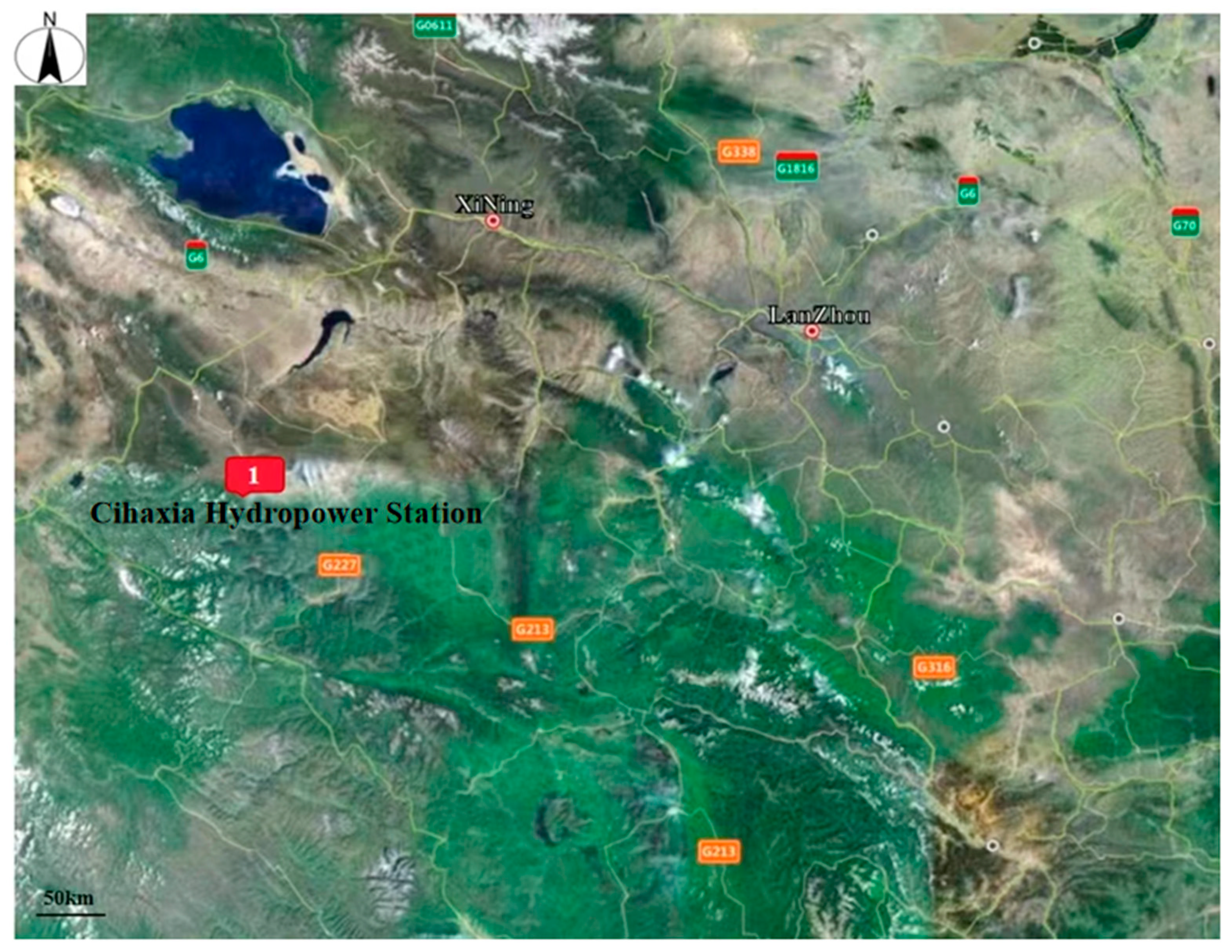
The 4# landslide of the Cihaxia hydropower station was selected as a case study in this work. At the upstream and downstream areas are Erduo and Banduo hydropower stations, respectively. The location of the Cihaxia hydropower station is shown in Figure 4(1). The dam is a concrete-faced sand and gravel rockfill dam. With a typical high water level of 2990 m. The installed capacity of the project is 2600 MW. The water release structures are located on the right bank, while the intake structure and diversion tunnel are located on the left bank. The engineering project was purposed for electricity generation.
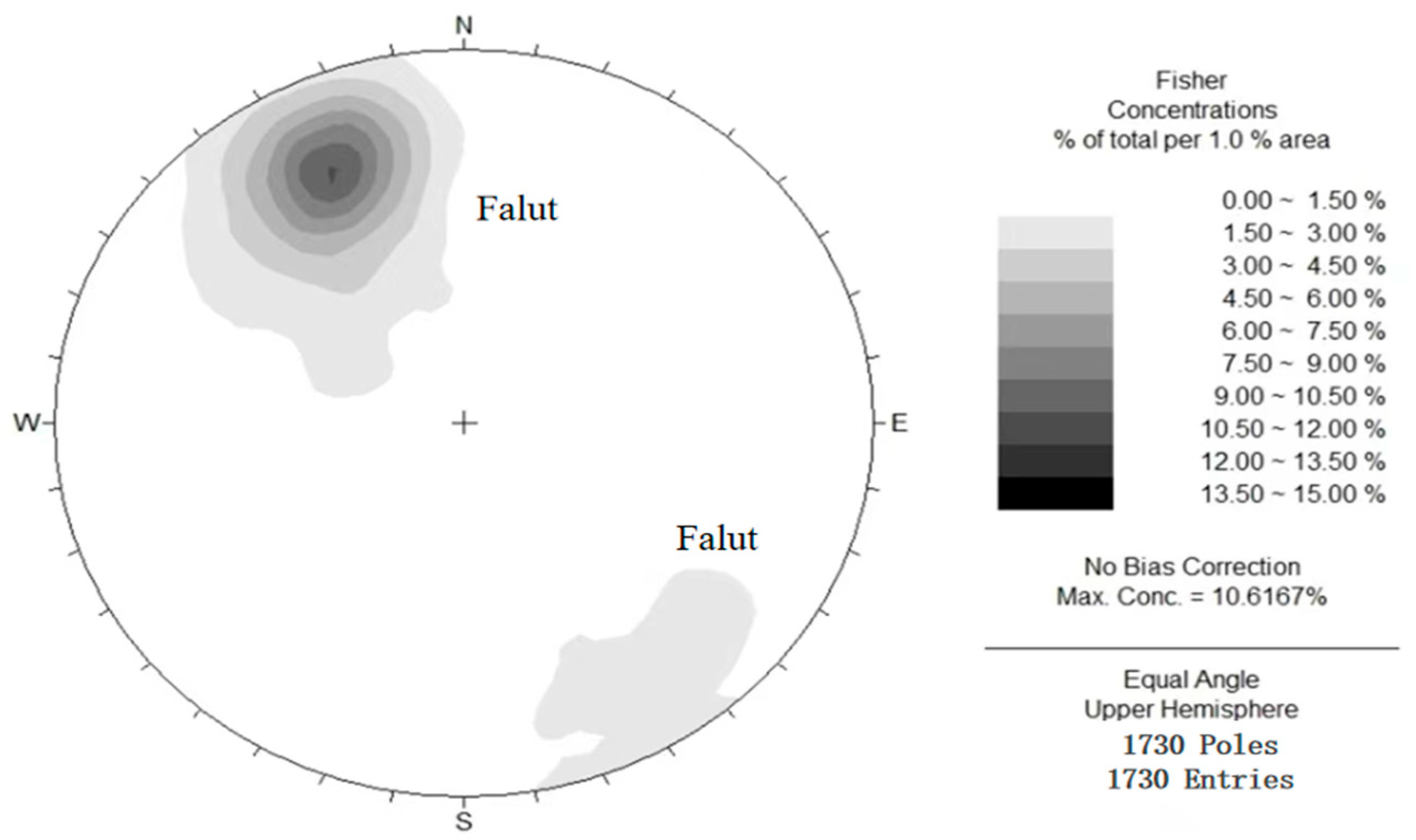
It can be observed from Figure 5 that the compression faults between the rock strata are the most developed, constituting two-thirds of all the faults. The occurrence of these faults is similar to that of the responding rock strata. Shear faults are the second most developed but have a scattered distribution, making it difficult to find them on the iso-density map. In the geological survey, the faults and fractures in the sandstone stratum (T2-Ss) are less than those in another stratum. In the rock stratum of slate, the number of faults increases, especially in the interlaminated sand slate rock strata. The faults develop along the boundary of the sand and slate. Meanwhile, more faults and fractures exist in a large scale in the landslide slope, which is caused by the shear movement of dipped rock.
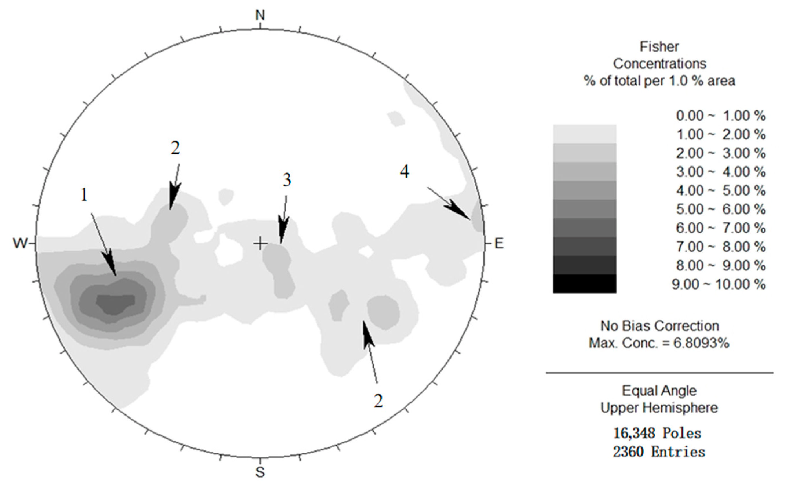
It can also be observed that the shallow faults between the rock strata are only less developed than the compression faults, which constitute one-third of all the faults. The shallow faults are of a large scale and have a long extension distance. All faults belong to four dominant groups. The groups were 1, 2, 3, and 4 in order of their dominant development, as shown in Figure 6.
The strike direction, dip azimuth, and dip angle of the first group of faults are NE10°–55°, SE(NW), and 65°–85°, respectively. The width of the faults zone is in the range of 5 cm–15 cm, and the maximum value of the width is 200 cm. The composition of the fault zone is mylonite, breccia, mudstone, and cataclasite. The surfaces of the faults’ rupture are smooth.
The second group comprises slightly inclined faults with a small scale, which are developed at the dam site. The width of the faults zone is in the range of 10 cm–25 cm. The composition of the fault zone is breccia, mudstone, and cataclasite. The extension distance of the faults’ rupture is short; however, two large faults, F1 and F27, are detected. F1 is detected in adit PD24, PD27, PD34, and PD40 while F27 is detected in adit PD10, PD21, and PD22. They are the control structures of the rock deformation and rock slope stability. The strike direction, dip azimuth and dip angle of F1 are NE18°–37°, NW, and 19°–25°, respectively. The width of the faults zone is in the range of 97 cm–500 cm. A fault gouge zone exists in the middle of the faults zone. Aside from the fault gouge zone, cataclasite, and rock cuttings are also present. The extension distance of the fault gouge zone is approximately 520 m. The strike direction, dip azimuth, and dip angle of F27 are NE13°–21°, NW, and 37°–41°, respectively. The width of the faults zone is in the range of 240 cm–510 cm. The composition of the fault zone is breccia, mudstone, and cataclasite, which are scattered in the zone. Striations are observed on the surfaces of faults’ rupture, and the extension distance of F27 is approximately 480 m. F27 is the control creep surface of the right bank at the dam site.
The third group comprises slightly inclined faults with high and middle dip angles and a small scale; these faults are developed at the dam site. The width of the faults zone is in the range of 10 cm–25 cm. The composition of the fault zone is breccia, mudstone, and cataclasite, which are slightly scattered, while the extension distance of the faults is short.
The fourth group comprises the least number of developed faults. The width of the faults zone is in the range of 5 cm–15 cm. The composition of the fault zone is cataclasite, breccia, mylonite, and mudstone.
The strata at the dam site are layered or thin-layered. The fractures are developed between the different strata, and the fractures are open because of geological processes. The width of the fractures is in the range of 2 mm–5 mm, with a maximum value of 10 mm. The composition of the fracture zone is rock power, rock cuttings, and mud with iron oxide red rust. The deep of the fractures is closed, and the occurrence of the fractures is the same as that of the responding strata. A total of 16,348 fractures are logged in the adits, and the groups of the fractures are illustrated in Figure 6.
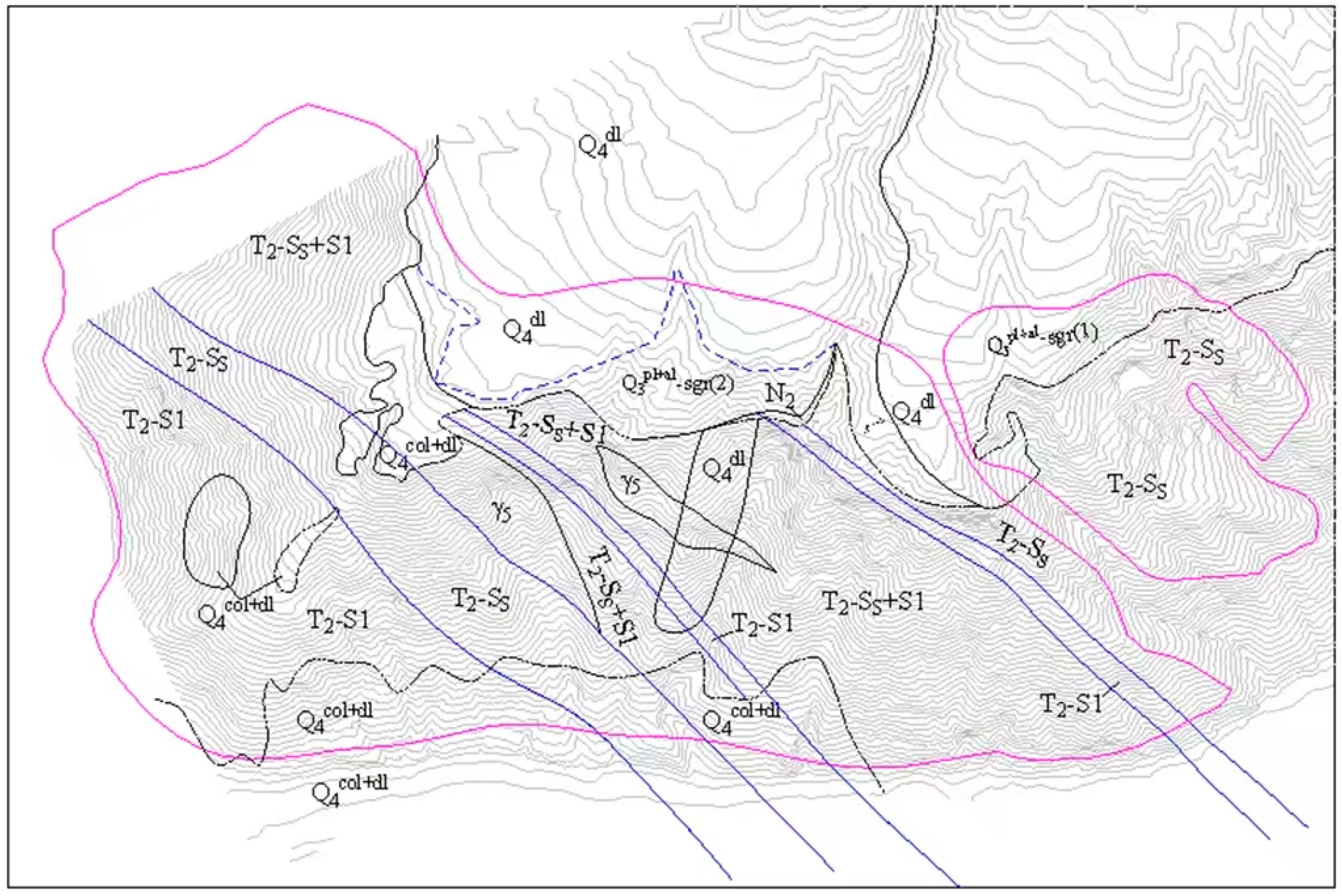
There are eight main strata in the landslide slope. Depending on the rock formation and the terrain, we divided it into different parts with color lines, and the lithology is shown in Figure 7.
- T2-Ss is a medium-thin layered sandstone mixed with slate. The sandstone is celadon to gray, medium-to-fine-textured, and layer-structured. The layer has a thickness in the range of 5 cm–25 cm; it is compacted, hard, and weather-resistant.
- T2-Ss + Sl: It is a celadon sandstone mixed up with a gray slate.
- T2-Sl is thin- to ultra-thin layered slate mixed with sandstone. The slate is gray to dark gray, medium-to-fine-textured, and layer-structured. The thickness of the layer is in the range of 0.5 cm–10 cm. The rock is relatively soft and not weather-resistant.
- The intermediate-acid intrusive dike of the Indo-Chinese epoch (γ5) is mainly composed of granite, quartz diorite, and quartzite. It is compacted, hard, and weather-resistant. It intrudes into the rock in the direction of the layer as a dike cutting the T2c stratum.
- The tertiary period Pliocene series (N2) is distributed on the top of the landslide slope, soft, and mainly composed of red-purple aleuropelitic rock. Unconformable contact exists between the stratum and the T2c layer.
- The epipleistocene gravel alluvium (Q3pl+al-sgr (2)) is distributed on the landslide slope far from the flat zone. It is mainly composed of sandstone, quartzite, granite, limestone, and slate. The stratum is dry, compacted, and slightly scattered.
- The holocene slope accumulation gravel soil (Q4dl) is distributed on the top of the landslide slope, which is mainly composed of sandstone and slate. The structure is scattered.
- The holocene avalanche slope accumulation block and rubble (Q4col+dl) is distributed over the bottom of the landslide slope, which is mainly composed of sandstone and slate of different sizes. The structure is scattered.
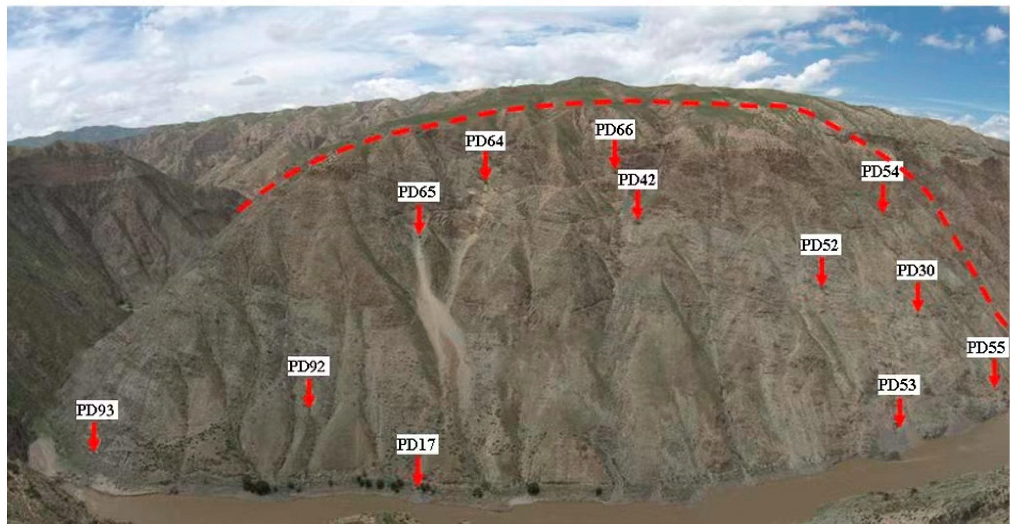
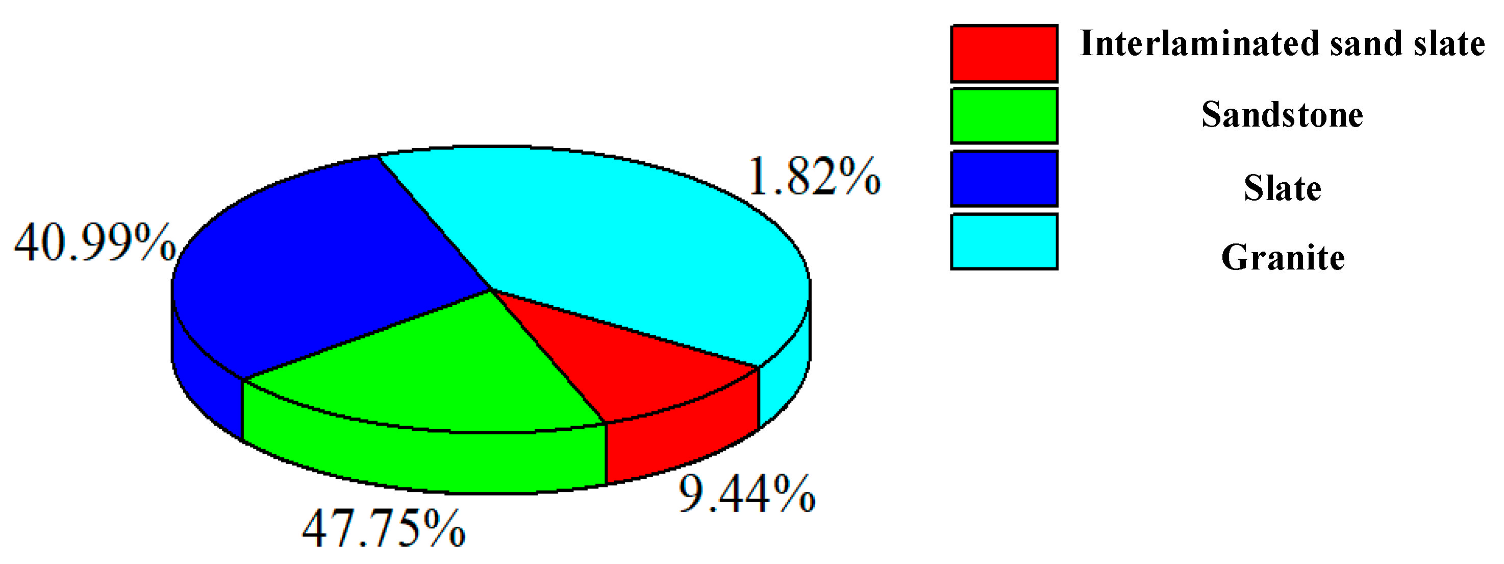
Results of the geological survey using adits (Figure 8) on the landslide slope are presented in Table 1. It can be seen from the table that the amount of sandstone and slate are similar, and the ratios are 47.75% and 40.99%, respectively. The ratio of interlaminated sand slate rock is 9.44%, and that of granite is 1.82%, as shown in Figure 9.
3.2. Slope Deformation Monitoring Using InSAR
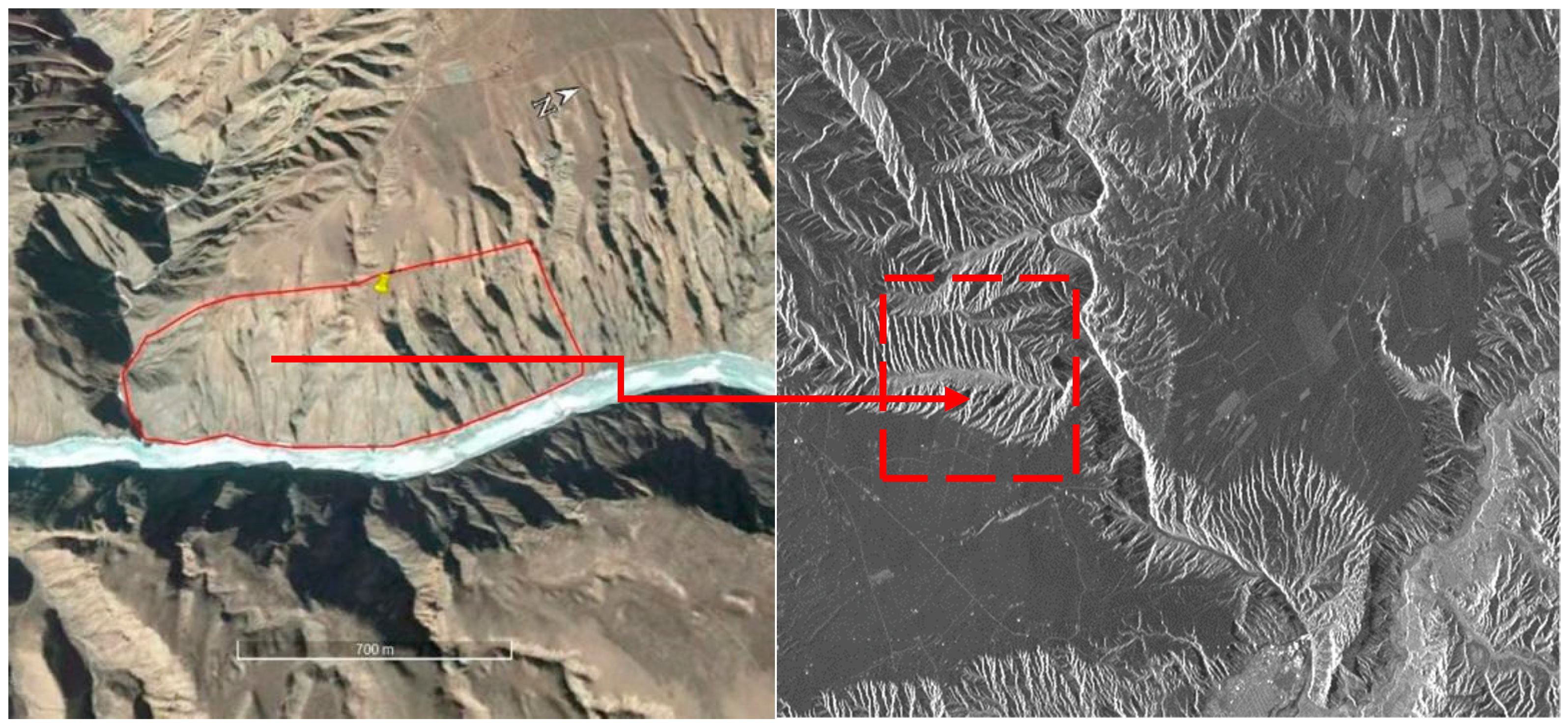
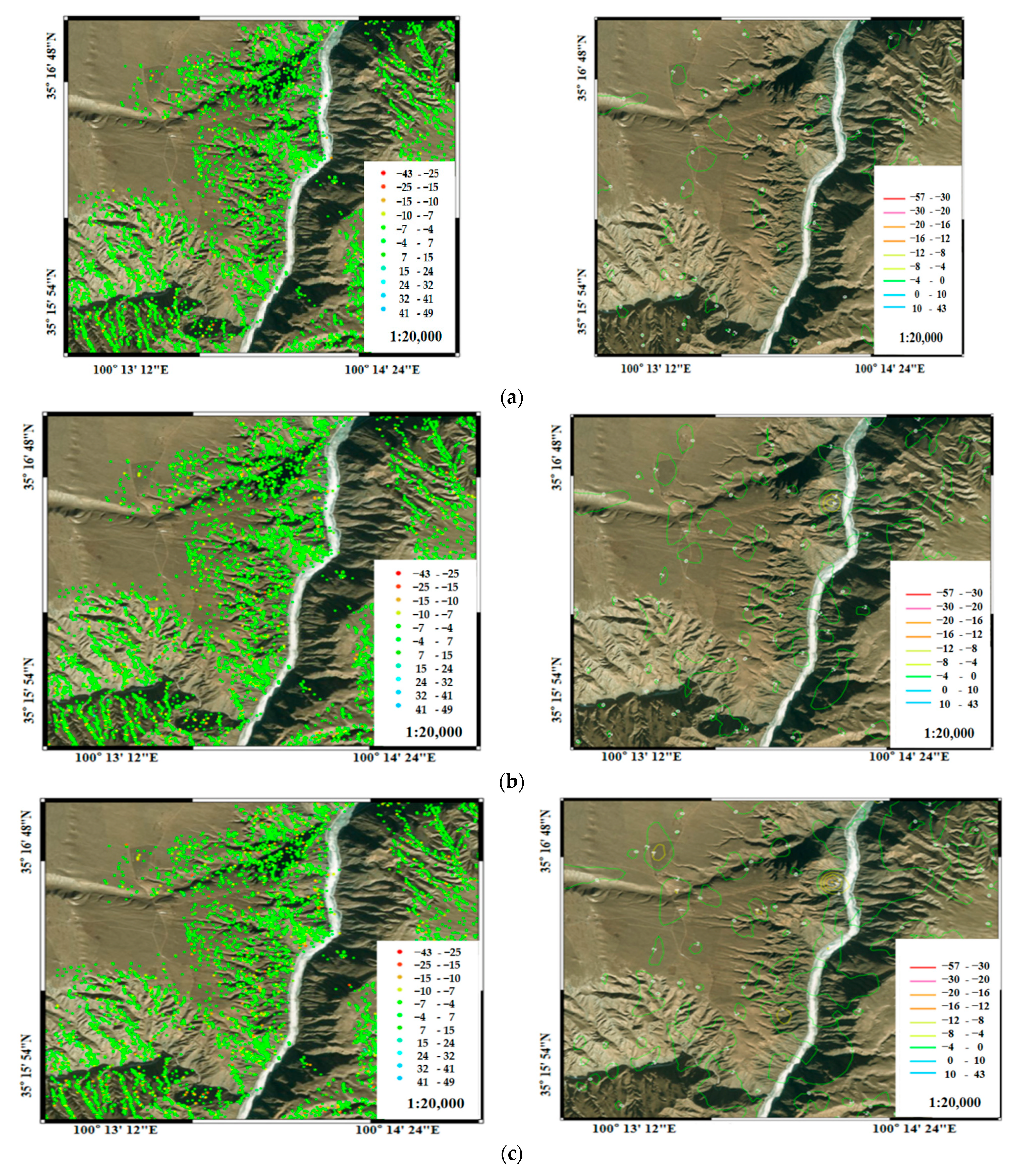
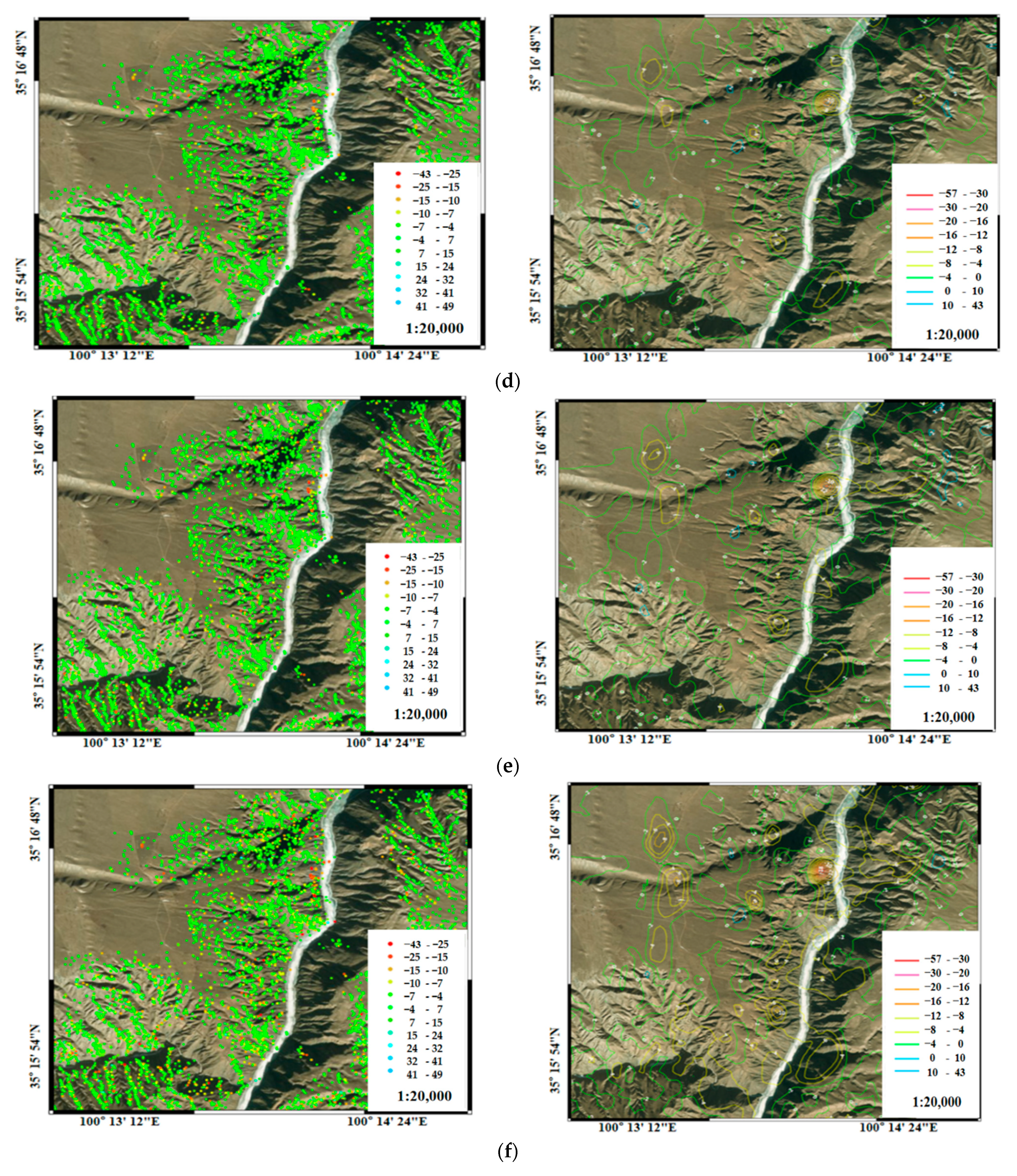
The remote sensing image of the slope (Figure 10) is from the Sentinel-1A data. The monitoring cycle is 12 days, and the incidence angle of the remote sensing satellite is 39.18°. The monitoring period is from October 2014 to August 2019, a total of five years. Figure 11 illustrates the comprehensive cumulative deformation distribution of the slope.
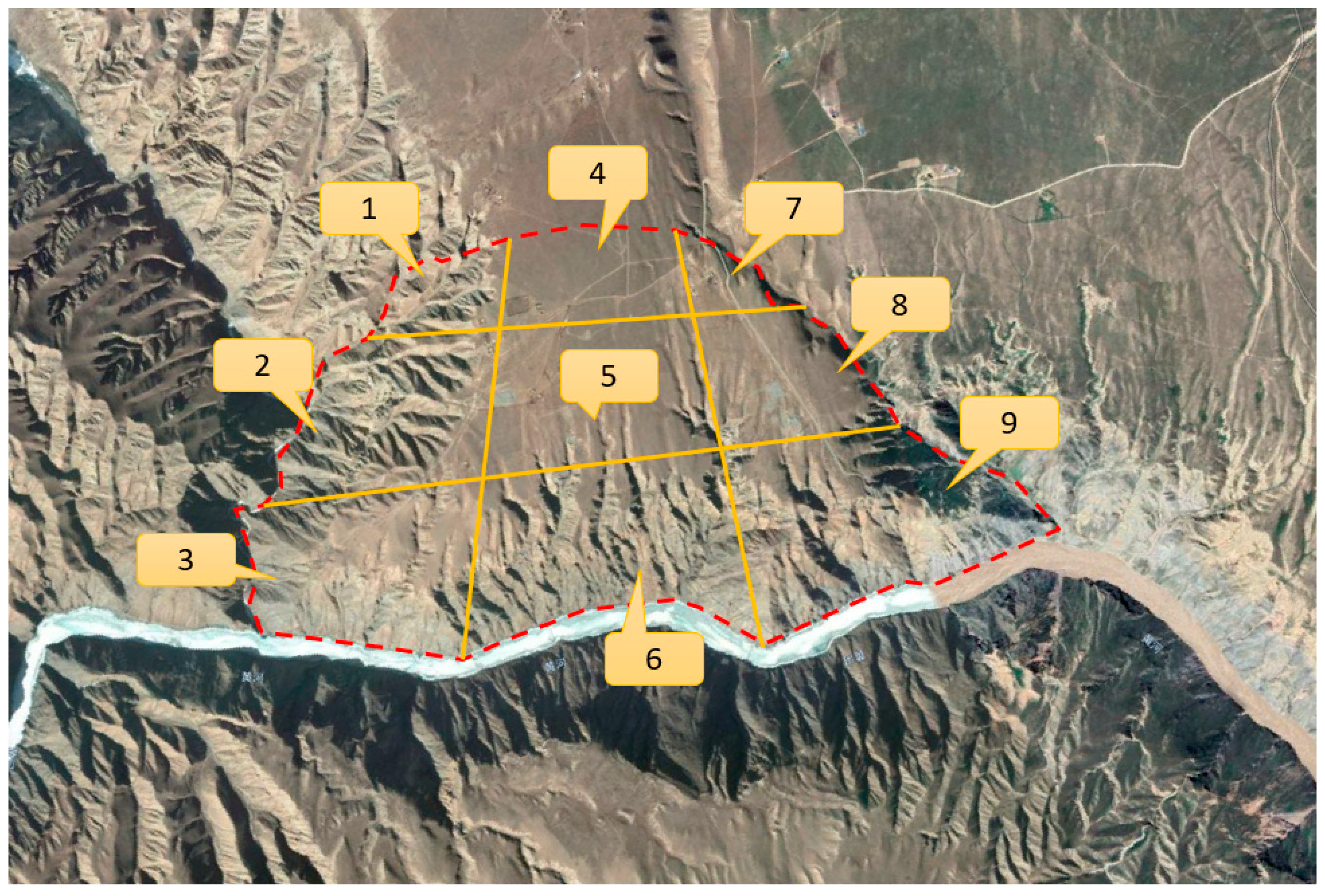
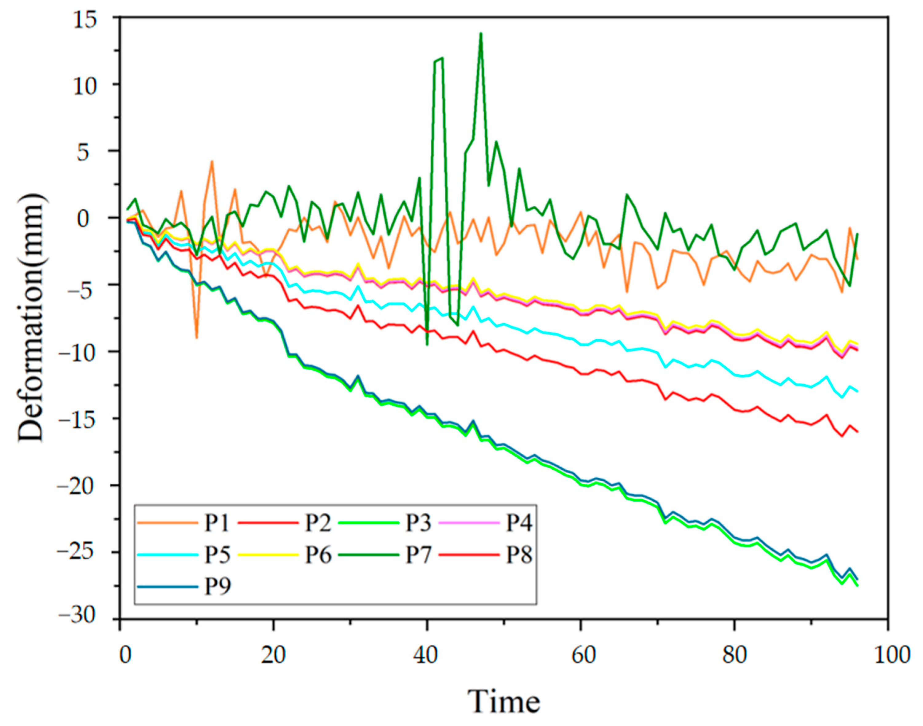
According to the monitoring results of the slope, we selected nine reference points in Figure 12 (1–9) to examine the deformation. The deformation statistic results of the corresponding points are shown in Figure 13.
Figure 13 shows that certain points have the same deformation pattern. For example, Points 1 and 7; Points 2, 4, and 6; and Points 3 and 9 have a similar deformation trend. Hence, we selected the deformation data of Points 1, 2, 5, 8, and 9 to conduct the study.
The raw data were first normalized: the maximum and minimum values were considered, and all the data were recalibrated to the range of [0, 1]. The normalization was performed using Equation (25).
where x is raw data and xn is normalized data; xmax and xmin are maximum and minimum data of the sequence, respectively.
After the normalization, the data were divided into training and testing datasets. The model was established using the training data and evaluated using the testing data. A reverse normalization was also performed using Equation (26) to process the prediction results.
where y is real prediction result and yn is result with normalization; ymax and ymin are the maximum and minimum prediction values of the sequence, respectively.
3.3. Experimental Results
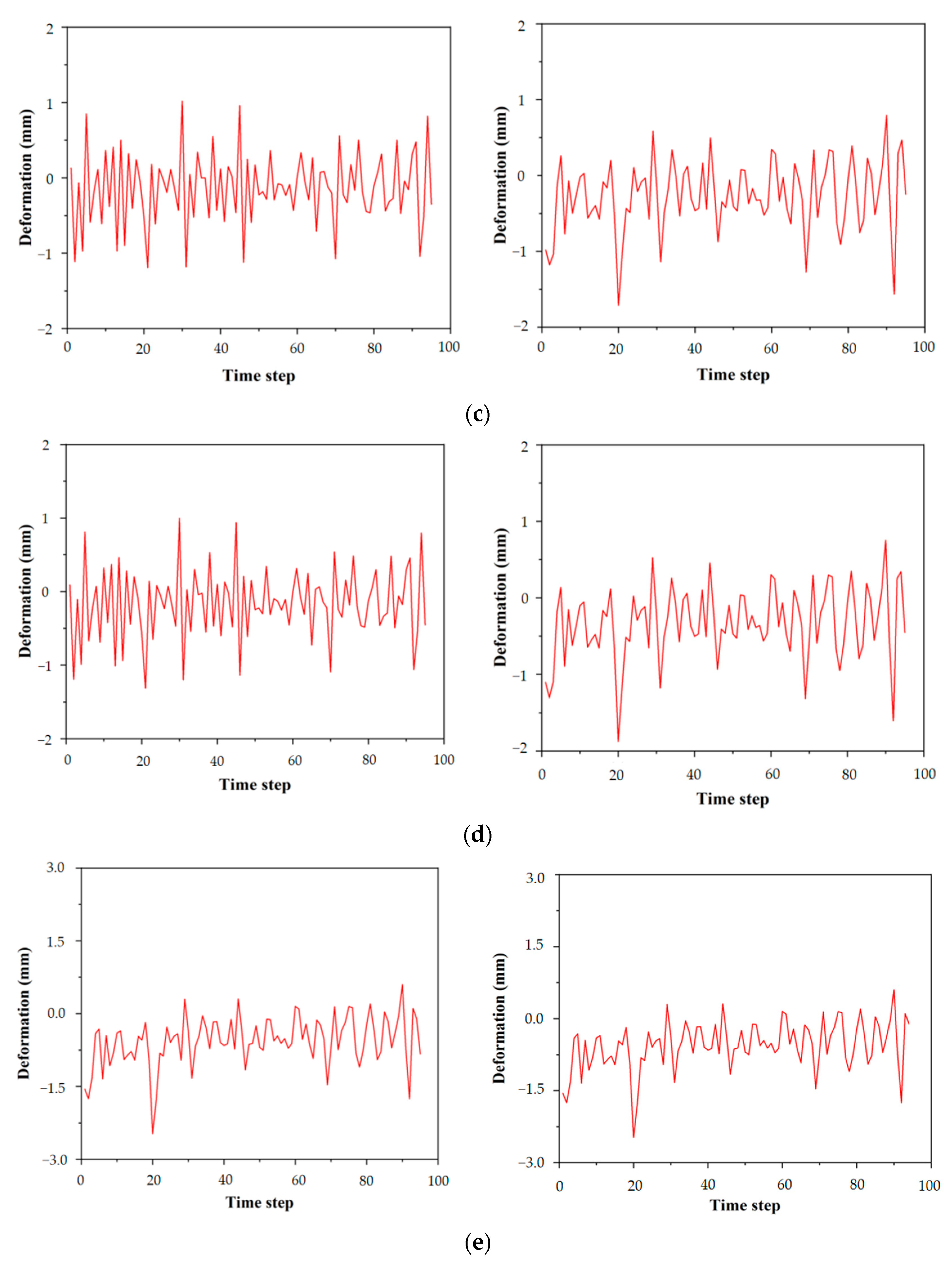
The ARIMA model was applied to first predict slope deformation. For the dataset, the monitored slope deformation data from November 2014 to November 2018 and from November 2018 to August 2019 were used as the training and testing data, respectively. Each time step represents an observation of the slope. RMSE, MAE, and R2 were used to evaluate the model. The first and second order differences were used to analyze the data sequence. The first order difference and second order difference were adopted to analyze the data sequence. The result of the first order difference and second order difference for the data sequence are shown in Figure 14.
As shown in Figure 14, the mean values of the deformation data mostly fluctuated about 0 after processing all the data sequences using the first and second differences. Meanwhile, the variances changed slightly. The results denote that the dataset of the five points is a stationary sequence.
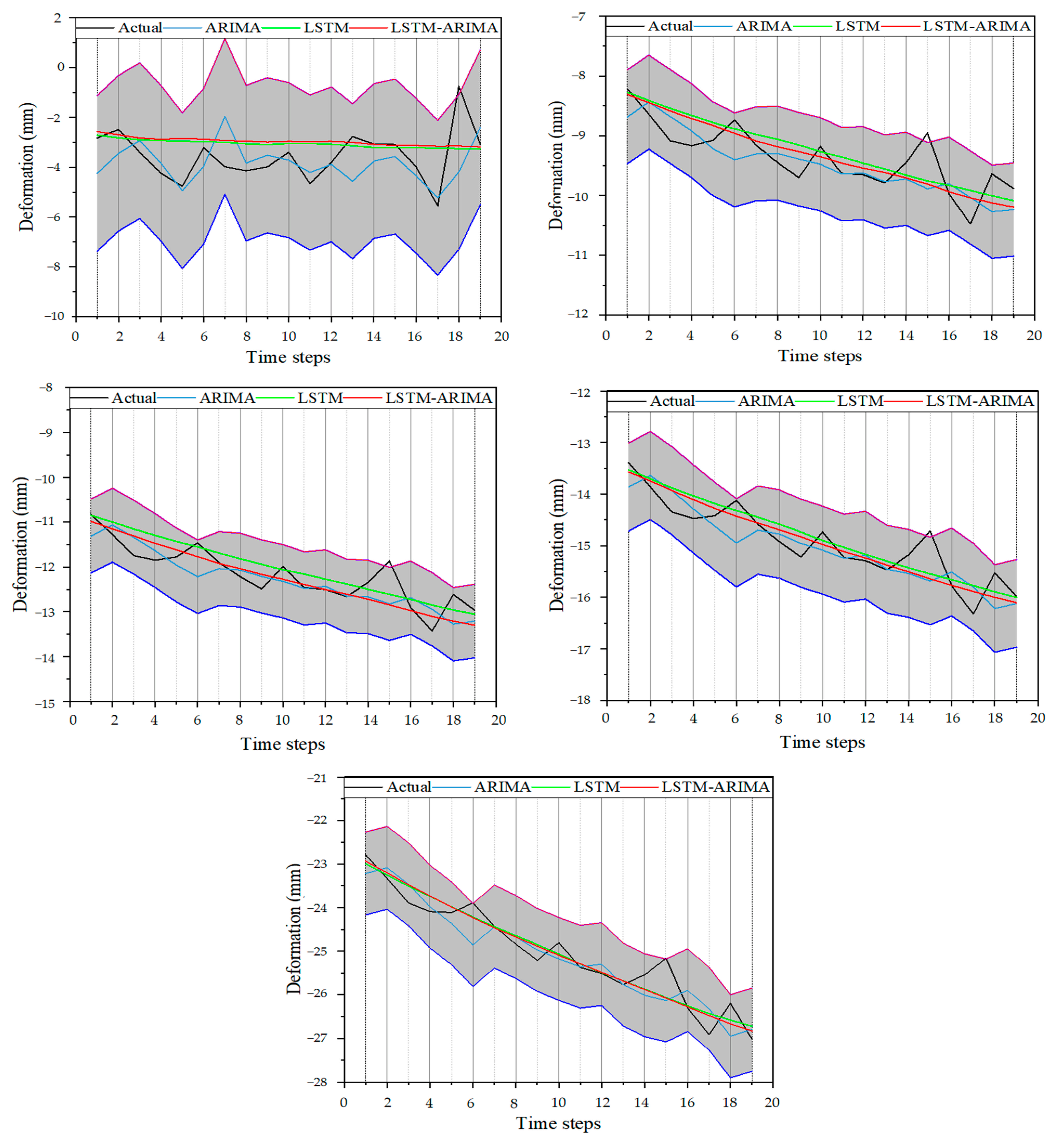
ARIMA, LSTM, and LSTM-ARIMA were used to build deformation prediction models. A confidence interval of 95% was used. In the model establishment phase, the ARIMA and LSTM models were built and evaluated first. The models’ establishment was based on the original data. The ARIMA model was then used to generate new features, which were added to the original data and fed to LSTM networks to build LSTM-ARIMA. The data sequence length of the LSTM was 10. The activation function of the dense layer was the tanh function, while Adam was selected as the optimizer; MSE was the loss function. The number of the LSTM units was 200, the number of epochs was 100, and the batch size was 128. The model performance was evaluated, and the prediction results were compared.
Table 2 shows that the LSTM-ARIMA model achieved outstanding performance among all the models. For Point 1, the data sequence pattern was difficult to determine. Although the sequence shown in Figure 10 appears stationary, the data sequence exhibits less regularity. The variances of the differences in the Point 1 data fluctuated in the range of (−5, 5) while that of other data fluctuated in the range of (−2, 2). Thus, it was unnecessary to improve the LSTM with the generated features using ARIMA. The R2 of the three models was negative, indicating poor fitting performance. For Points 2, 5, and 8, LSTM-ARIMA outperformed LSTM and ARIMA, indicating that the new features generated by ARIMA were effective for model establishment. For Point 9, LSTM-ARIMA performed slightly better than LSTM, indicating that the features generated by ARIMA were not always effective. The features generated by ARIMA provided the pseudo-values for model training, depending on the accuracy of the features. Therefore, accurate feature generation is significant for model establishment.
Figure 15 illustrates the actual data sequence and predicted results of ARIMA, LSTM, and LSTM-ARIMA. The upper and lower boundaries of the 95% confidence interval are also illustrated, and the gray area between the upper and lower boundaries of the 95% confidence interval. The time steps refer to the time at which the slope deformation was monitored using InSAR. All the prediction points are in the gray zones, which can be used to predict the trend and bias using ARIMA. However, a contrary trend can also be predicted by ARIMA, causing a significant error. Thus, the mean trend was predicted using LSTM and LSTM-ARIMA. For Point 1, the trend was nearly 0, and the prediction performance was poor. The data trends of the five points were similar, and the models had a similar performance, indicating that the proposed model is robust.
3.4. Discussion
In this study, we proposed an ensemble model based on LSTM and ARIMA. Considering the differences among the observed points, five points in different zones were selected to establish the model. The model performance evaluation results showed that the LSTM and LSTM-ARIMA models accurately predicted the trend in the data sequence. The RMSE and MAE of both models were smaller than those of ARIMA for most points. Meanwhile, the new features generated using ARIMA improved the LSTM performance. The models based on the data of Points 2, 5, and 8 data have shown the result. For the model based on Point 1, the performance of LSTM-ARIMA was worse than that of the other two models. For the model based on Point 9, the performance of LSTM was better than that of LSTM-ARIMA. The results indicate the need for generated features to be accurate; otherwise, they would be unsuitable for LSTM-ARIMA mode establishment.
However, as noted in the previous subsection, the data sequence of the five points had certain similarities. Thus, the regularity of the various model performances was similar. The LSTM and LSTM-ARIMA models identified the patterns of the data sequence trend; however, the models were not sensitive to the bias of the data sequence. Considering this limitation, the model performance should be validated on more data sequences in future studies to demonstrate its robustness. Meanwhile, the improvement obtained from using ARIMA was limited. Similarly, more AR models should be considered in time series feature generation. We found that more effective features are significant for model establishment; therefore, more effective features obtained using AR models should be added to datasets to build prediction models in future studies.
4. Conclusions
LSTM is frequently used to predict landslide deformation. Xie et al. [45] used LSTM to predict the periodic component of landslide deformation and found that LSTM has a good dynamic prediction performance. Gao et al. [46] used the LSTM-TAR model to predict landslide displacement, and found that the proposed combination model has high accuracy. Yang et al. [47] used the SSA algorithm to optimize the hyper-parameters of the LSTM neural network, which achieved a high-precision prediction of LSTM landslide displacement. Therefore, we proposed the LSTM-ARIMA slope deformation prediction model using ensemble features; the model is based on LSTM and ARIMA. The LSTM model identifies the trend in the data sequence with time while ARIMA predicts the bias of the stationary data sequence. Combining the advantages of both approaches, our proposed LSTM-ARIMA model effectively identifies the trend in landslide deformation data. The feasibility and superiority of the model were demonstrated by applying them to an actual engineering project and comparing their performance with that of LSTM and ARIMA individually on the same datasets. The main findings and contributions of this work are summarized as follows:
- The slope deformation was recorded using InSAR, and all the points on the map were recorded. The selected points in different zones were used as the study data. A geological survey provided the engineering details for the composition of the whole slope.
- LSTM predicts the trend in time series data but is insensitive to deviations in data series. Because ARIMA effectively predicts the deviation of stationary sequences, we selected the predictions of ARIMA as new features and added them to the original data as an input to the LSTM. This approach improved the prediction performance of LSTM.
- From the analysis results, the LSTM and LSTM-ARIMA models effectively predicted the slope deformation trend, and for most data points, the LSTM-ARIMA model had minimal RMSE and MAE. Using the ARIMA model to predict the data series yielded a large error, but adding the prediction as a new feature to the original data improved the prediction performance of the ensemble model. In the future, features generated by the ARIMA model can be added to the raw data as pseudo-data to enhance the predictive performance of the model.
According to the InSAR monitoring technique, the proposed method can determine the trend in landslide deformation data, making it suitable for landslide slope prediction in engineering. Furthermore, the deformation of the landslide slope is not stopping in Cihaxia engineering. When the prediction error increases, we need to determine whether the deformation changes rapidly or stops gradually. Thus, the prediction our model achieves provides a new perspective for processing landslide slope deformation data.
Author Contributions
Y.W.: Methodology and Writing—original draft. S.L.: Data curation and Writing—review and editing. B.L.: Conceptualization and Coding. All authors have read and agreed to the published version of the manuscript.
Funding
This research was funded by the Key Laboratory of Port Geotechnical Engineering, Ministry of Communications, PRC (Grand No. 2021-11-073-1206).
Data Availability Statement
Data generated and analyzed during this study are available from the corresponding author by request.
Conflicts of Interest
The authors declare that they have no known competing financial interests or personal relationships that could have appeared to influence the work reported in this paper.
References
- Zhang, Z.; Liu, G.; Wu, S.; Tang, H.; Wang, T.; Li, G.; Liang, C. Rock slope deformation mechanism in the Cihaxia hydropower station, Northwest China. Bull. Eng. Geol. Environ. 2015, 74, 943–958. [Google Scholar] [CrossRef]
- Zhang, Z.; Wang, T.; Wu, S.; Tang, H. Rock toppling failure mode influenced by local response to earthquakes. Bull. Eng. Geol. Environ. 2016, 75, 1361–1375. [Google Scholar] [CrossRef]
- Yan, G.; Yin, Y.; Huang, B.; Zhang, Z.; Zhu, S. Formation mechanism and characteristics of the Jinjiling landslide in Wushan in the Three Gorges Reservoir region, China. Landslides 2019, 16, 2087–2101. [Google Scholar] [CrossRef]
- Kim, J.; Kim, Y.; Jeong, S.; Hong, M. Rainfall-induced landslides by deficit field matric suction in unsaturated soil slopes. Environ. Earth Sci. 2017, 76, 1–17. [Google Scholar] [CrossRef]
- Cogan, J.; Gratchev, I. A study on the effect of rainfall and slope characteristics on landslide initiation by means of flume tests. Landslides 2019, 16, 2369–2379. [Google Scholar] [CrossRef]
- Cuomo, S.; Di Perna, A.; Martinelli, M. Modelling the spatio-temporal evolution of a rainfall-induced retrogressive landslide in an unsaturated slope. Eng. Geol. 2021, 294, 106371. [Google Scholar] [CrossRef]
- Castro, J.; Asta, M.P.; Galve, J.P.; Azañón, J.M. Formation of clay-rich layers at the slip surface of slope instabilities: The role of groundwater. Water 2020, 12, 2639. [Google Scholar] [CrossRef]
- Marino, P.; Santonastaso, G.F.; Fan, X.; Greco, R. Prediction of shallow landslides in pyroclastic-covered slopes by coupled modeling of unsaturated and saturated groundwater flow. Landslides 2021, 18, 31–41. [Google Scholar] [CrossRef]
- Marc, V.; Bertrand, C.; Malet, J.-P.; Carry, N.; Simler, R.; Cervi, F. Groundwater—Surface waters interactions at slope and catchment scales: Implications for landsliding in clay-rich slopes. Hydrol. Process. 2017, 31, 364–381. [Google Scholar] [CrossRef]
- Gao, W.W.; Gao, W.; Hu, R.L.; Xu, P.F.; Xia, J.G. Microtremor survey and stability analysis of a soil-rock mixture landslide: A case study in Baidian town, China. Landslides 2018, 15, 1951–1961. [Google Scholar] [CrossRef]
- Zhang, C.; Zhang, M.; Zhang, T.; Dai, Z.; Wang, L. Influence of intrusive granite dyke on rainfall-induced soil slope failure. Bull. Eng. Geol. Environ. 2020, 79, 5259–5276. [Google Scholar] [CrossRef]
- Kim, K.-S.; Jeong, S.-W.; Song, Y.-S.; Kim, M.; Park, J.-Y. Four-year monitoring study of shallow landslide hazards based on hydrological measurements in a weathered granite soil slope in South Korea. Water 2021, 13, 2330. [Google Scholar] [CrossRef]
- Zheng, Y.; Zhu, Z.W.; Li, W.J.; Gu, D.M.; Xiao, W. Experimental research on a novel optic fiber sensor based on OTDR for landslide monitoring. Measurement 2019, 148, 106926. [Google Scholar] [CrossRef]
- Wu, H.; Guo, Y.; Xiong, L.; Liu, W.; Li, G.; Zhou, X. Optical fiber-based sensing, measuring, and implementation methods for slope deformation monitoring: A review. IEEE Sens. J. 2019, 19, 2786–2800. [Google Scholar] [CrossRef]
- Hong, C.-Y.; Zhang, Y.-F.; Li, G.-W.; Zhang, M.-X.; Liu, Z.-X. Recent progress of using Brillouin distributed fiber optic sensors for geotechnical health monitoring. Sens. Actuators A Phys. 2017, 258, 131–145. [Google Scholar] [CrossRef]
- Parente, L.; Chandler, J.H.; Dixon, N. Optimising the quality of an SfM-MVS slope monitoring system using fixed cameras. Photogramm. Rec. 2019, 34, 408–427. [Google Scholar] [CrossRef]
- Li, Q.; Min, G.; Chen, P.; Liu, Y.; Tian, S.; Zhang, D.; Zhang, W. Computer vision-based techniques and path planning strategy in a slope monitoring system using unmanned aerial vehicle. Int. J. Adv. Robot. Syst. 2020, 17, 1729881420904303. [Google Scholar] [CrossRef]
- Li, H.-B.; Li, X.-W.; Li, W.-Z.; Zhang, S.-L.; Zhou, J.-W. Quantitative assessment for the rockfall hazard in a post-earthquake high rock slope using terrestrial laser scanning. Eng. Geol. 2019, 248, 1–13. [Google Scholar] [CrossRef]
- Li, H.-B.; Qi, S.-C.; Yang, X.-G.; Li, X.-W.; Zhou, J.-W. Geological survey and unstable rock block movement monitoring of a post-earthquake high rock slope using terrestrial laser scanning. Rock Mech. Rock Eng. 2020, 53, 4523–4537. [Google Scholar] [CrossRef]
- Sun, Q.; Zhang, L.; Ding, X.; Hu, J.; Li, Z.; Zhu, J. Slope deformation prior to Zhouqu, China landslide from InSAR time series analysis. Remote Sens. Environ. 2015, 156, 45–57. [Google Scholar] [CrossRef]
- Zhang, Y.; Meng, X.; Jordan, C.; Novellino, A.; Dijkstra, T.; Chen, G. Investigating slow-moving landslides in the Zhouqu region of China using InSAR time series. Landslides 2018, 15, 1299–1315. [Google Scholar] [CrossRef]
- Dai, C.; Li, W.; Wang, D.; Lu, H.; Xu, Q.; Jian, J. Active landslide detection based on Sentinel-1 data and InSAR technology in Zhouqu county, Gansu province, Northwest China. J. Earth Sci. 2021, 32, 1092–1103. [Google Scholar] [CrossRef]
- Tang, Y.; Feng, F.; Guo, Z.; Feng, W.; Li, Z.; Wang, J.; Sun, Q.; Ma, H.; Li, Y. Integrating principal component analysis with statistically-based models for analysis of causal factors and landslide susceptibility mapping: A comparative study from the loess plateau area in Shanxi (China). J. Clean. Prod. 2020, 277, 124159. [Google Scholar] [CrossRef]
- Li, S.H.; Wu, L.Z.; Chen, J.J.; Huang, R. Multiple data-driven approach for predicting landslide deformation. Landslides 2020, 17, 709–718. [Google Scholar] [CrossRef]
- Shahabi, H.; Hashim, M.; Ahmad, B.B. Remote sensing and GIS-based landslide susceptibility mapping using frequency ratio, logistic regression, and fuzzy logic methods at the central Zab basin, Iran. Environ. Earth Sci. 2015, 73, 8647–8668. [Google Scholar] [CrossRef]
- Du, S.; Zhang, J.; Li, J.; Su, Q.; Zhu, W.; Chen, Y. The deformation prediction of mine slope surface using PSO-SVM model. TELKOMNIKA Indones. J. Electr. Eng. 2013, 11, 7182–7189. [Google Scholar] [CrossRef]
- Yu, C.; Chen, J. Landslide susceptibility mapping using the slope unit for southeastern Helong City, Jilin Province, China: A comparison of ANN and SVM. Symmetry 2020, 12, 1047. [Google Scholar] [CrossRef]
- Zhang, L.; Shi, B.; Zhu, H.; Yu, X.B.; Han, H.; Fan, X. PSO-SVM-based deep displacement prediction of Majiagou landslide considering the deformation hysteresis effect. Landslides 2021, 18, 179–193. [Google Scholar] [CrossRef]
- Hu, X.; Wu, S.; Zhang, G.; Zheng, W.; Liu, C.; He, C.; Liu, Z.; Guo, X.; Zhang, H. Landslide displacement prediction using kinematics-based random forests method: A case study in Jinping Reservoir Area, China. Eng. Geol. 2021, 283, 105975. [Google Scholar] [CrossRef]
- Sun, D.; Wen, H.; Wang, D.; Xu, J. A random forest model of landslide susceptibility mapping based on hyperparameter optimization using Bayes algorithm. Geomorphology 2020, 362, 107201. [Google Scholar] [CrossRef]
- Chen, H.; Zeng, Z. Deformation prediction of landslide based on improved back-propagation neural network. Cogn. Comput. 2013, 5, 56–62. [Google Scholar] [CrossRef]
- Gordan, B.; Armaghani, D.J.; Hajihassani, M.; Monjezi, M. Prediction of seismic slope stability through combination of particle swarm optimization and neural network. Eng. Comput. 2016, 32, 85–97. [Google Scholar] [CrossRef]
- Javdanian, H.; Pradhan, B. Assessment of earthquake-induced slope deformation of earth dams using soft computing techniques. Landslides 2019, 16, 91–103. [Google Scholar] [CrossRef]
- Zhang, N.; Zhang, W.; Liao, K.; Zhu, H.-H.; Li, Q.; Wang, J. Deformation prediction of reservoir landslides based on a Bayesian optimized random forest-combined Kalman filter. Environ. Earth Sci. 2022, 81, 1–14. [Google Scholar] [CrossRef]
- Deng, L.; Smith, A.; Dixon, N.; Yuan, H. Machine learning prediction of landslide deformation behaviour using acoustic emission and rainfall measurements. Eng. Geol. 2021, 293, 106315. [Google Scholar] [CrossRef]
- Garg, N.; Soni, K.; Saxena, T.; Maji, S. Applications of AutoRegressive Integrated Moving Average (ARIMA) approach in time-series prediction of traffic noise pollution. Noise Control Eng. J. 2015, 63, 182–194. [Google Scholar] [CrossRef] [Green Version]
- Hu, A.Y.; Bao, T.F.; Yang, C.L. LSTM-ARIMA-based Prediction of Dam Deformation: Model and Its Application. J. Yangtze River Sci. Res. Inst. 2020, 37, 64–68. [Google Scholar]
- Chen, H.; Zeng, Z.; Tang, H. Landslide deformation prediction based on recurrent neural network. Neural Process. Lett. 2015, 41, 169–178. [Google Scholar] [CrossRef]
- Yang, B.; Yin, K.; Lacasse, S.; Liu, Z. Time series analysis and long short-term memory neural network to predict landslide displacement. Landslides 2019, 16, 677–694. [Google Scholar] [CrossRef]
- Zhang, W.; Li, H.; Tang, L.; Gu, X.; Wang, L.; Wang, L. Displacement prediction of Jiuxianping landslide using gated recurrent unit (GRU) networks. Acta Geotech. 2022, 17, 1367–1382. [Google Scholar] [CrossRef]
- Wang, J.; Nie, G.; Gao, S.; Wu, S.; Li, H.; Ren, X. Landslide Deformation Prediction Based on a GNSS Time Series Analysis and Recurrent Neural Network Model. Remote Sens. 2021, 13, 1055. [Google Scholar] [CrossRef]
- Jiang, H.; Li, Y.; Zhou, C.; Hong, H.; Glade, T.; Yin, K. Landslide Displacement Prediction Combining LSTM and SVR Algorithms: A Case Study of Shengjibao Landslide from the Three Gorges Reservoir Area. Appl. Sci. 2020, 10, 7830. [Google Scholar] [CrossRef]
- Xing, Y.; Yue, J.; Chen, C. Interval Estimation of Landslide Displacement Prediction Based on Time Series Decomposition and Long Short-Term Memory Network. IEEE Access 2020, 8, 3187–3196. [Google Scholar] [CrossRef]
- Zhang, X.; Zhu, C.; He, M.; Dong, M.; Zhang, G.; Zhang, F. Failure Mechanism and Long Short-Term Memory Neural Network Model for Landslide Risk Prediction. Remote Sens. 2022, 14, 166. [Google Scholar] [CrossRef]
- Xie, P.; Zhou, A.; Chai, B. The Application of Long Short-Term Memory(LSTM) Method on Displacement Prediction of Multifactor-Induced Landslides. IEEE Access 2019, 7, 54305–54311. [Google Scholar] [CrossRef]
- Gao, Y.; Chen, X.; Tu, R.; Chen, G.; Luo, T.; Xue, D. Prediction of Landslide Displacement Based on the Combined VMD-Stacked LSTM-TAR Model. Remote Sens. 2020, 14, 1164. [Google Scholar] [CrossRef]
- Yang, S.; Jin, A.; Nie, W.; Liu, C.; Li, Y. Research on SSA-LSTM-Based Slope Monitoring and Early Warning Model. Sustainability 2022, 14, 10246. [Google Scholar] [CrossRef]
Figure 1.
Overall framework and flowchart.

Figure 2.
Model for InSAR interferometric geometry.

Figure 3.
The structure of a LSTM cell.

Figure 4.
The location of Cihaxia Hydropower Station.

Figure 5.
Iso-density map of fault poles in the dam site area.

Figure 6.
Iso-density map of fissure poles in the dam site area (excluding layer fissures).

Figure 7.
The lithology of the slope of the typical dumping body on the left bank.

Figure 8.
Layout of a typical dumping body exploration flat.

Figure 9.
Lithology statistics of the slope adits on the left bank.

Figure 10.
Remote sensing image of the slope.

Figure 11.
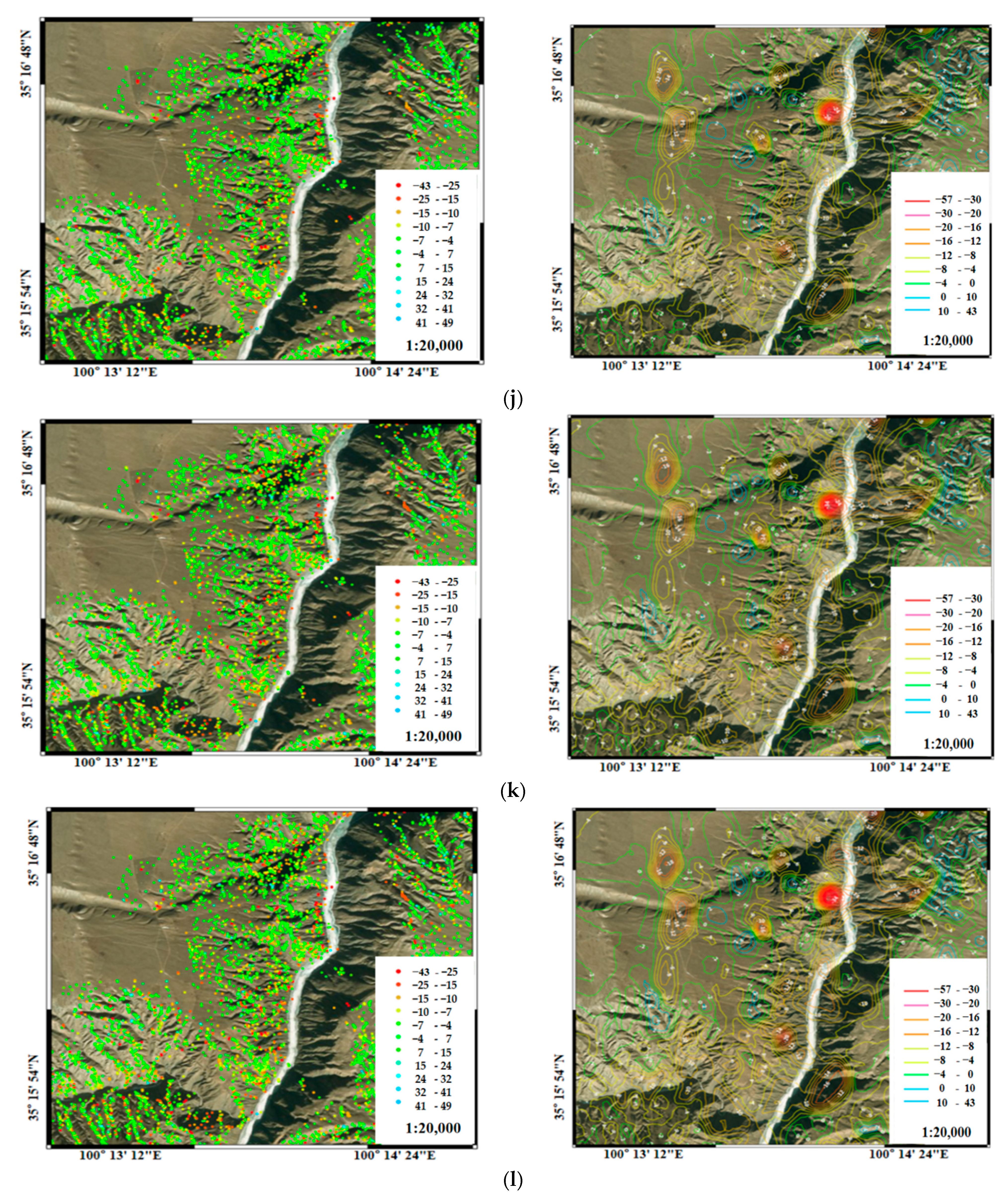
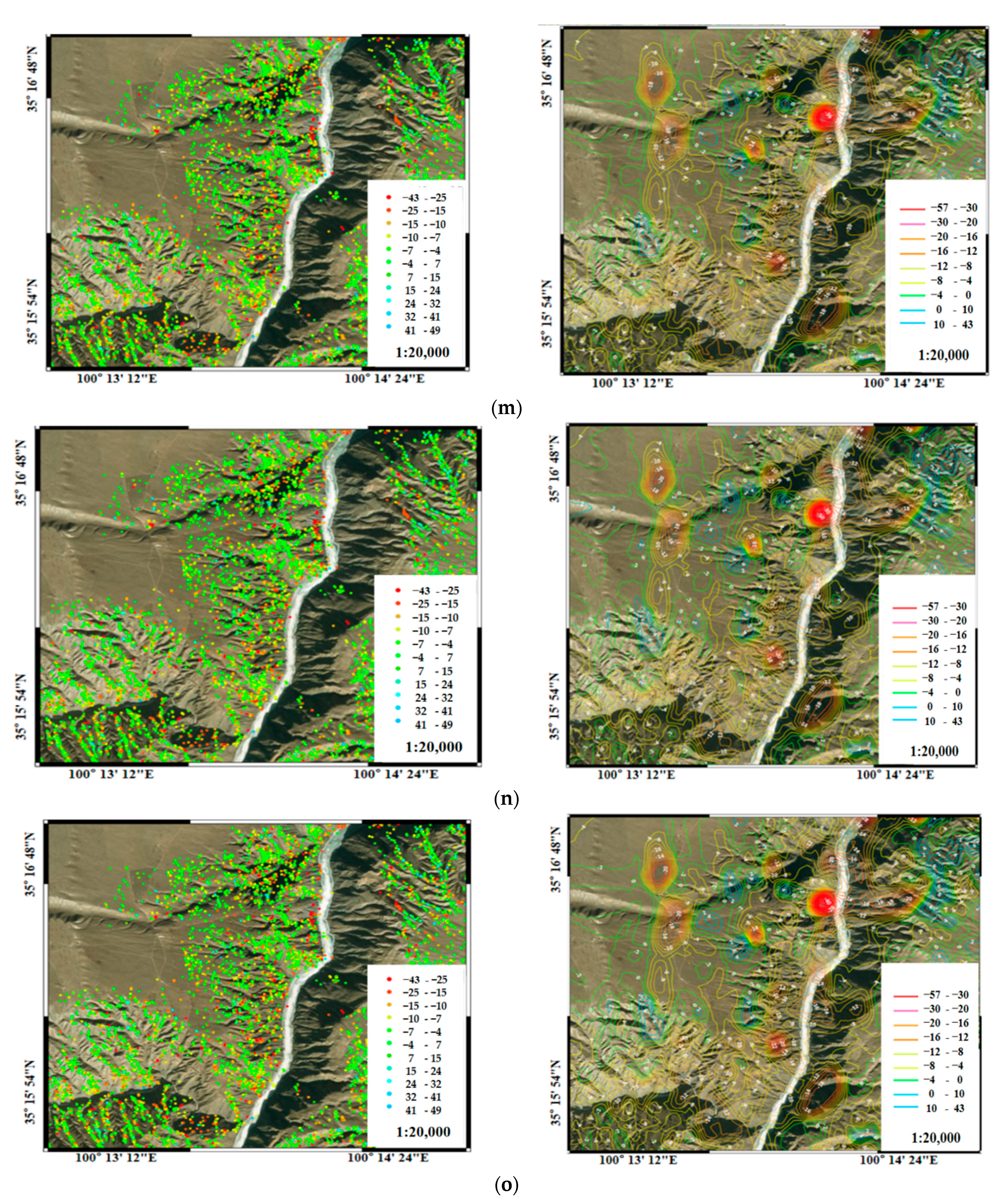
Cumulative deformation distribution map of the slope. (a) As of January 2015; (b) As of May 2015; (c) As of August 2015; (d) As of December 2015; (e) As of March 2016; (f) As of August 2016; (g) As of November 2016; (h) As of April 2017; (i) As of August 2017; (j) As of February 2018; (k) As of June 2018; (l) As of October 2018; (m) As of February 2019; (n) As of May 2019; (o) As of August 2019.
Figure 11.
Cumulative deformation distribution map of the slope. (a) As of January 2015; (b) As of May 2015; (c) As of August 2015; (d) As of December 2015; (e) As of March 2016; (f) As of August 2016; (g) As of November 2016; (h) As of April 2017; (i) As of August 2017; (j) As of February 2018; (k) As of June 2018; (l) As of October 2018; (m) As of February 2019; (n) As of May 2019; (o) As of August 2019.


Figure 12.
Typical measuring point distribution diagram.

Figure 13.
Deformation curve with time of typical points.

Figure 14.
First difference and second difference for the data of five points. (a) First difference and second difference for Point 1; (b) First difference and second difference for Point 2; (c) First difference and second difference for Point 5; (d) First difference and second difference for Point 8; (e) First difference and second difference for Point 9.


Figure 15.
The performance comparison of ARIMA, LSTM, and LSTM−ARIMA models.


Table 1.
Summary of lithological distribution of the slope.
| PD17 | PD55 | ||||
| Chainage (m) | Lithology | Thickness (m) | Chainage (m) | Lithology | Thickness (m) |
| 0–26 | Quaternary system accumulation | 26 | 0–5.6 | Slate | 5.6 |
| 26–32.5 | Slate | 6.5 | 5.6–7.5 | Sandstone | 1.9 |
| 32.5–34.2 | Sandstone | 1.7 | 7.5–8.5 | Slate | 1 |
| 34.2–36.8 | Slate | 2.6 | 8.5–15.5 | Sandstone | 7 |
| 36.8–38.7 | Sandstone | 1.9 | 15.5–21 | Slate | 5.5 |
| 38.7–40 | Slate | 1.3 | 21–22.7 | Sandstone | 1.7 |
| 40–44.2 | Sandstone | 4.2 | 22.7–30.1 | Slate | 7.4 |
| 44.2–46.7 | Slate | 2.5 | 30.1–31.6 | Sandstone | 1.5 |
| 46.7–53 | Sandstone | 6.3 | 31.6–36 | Slate | 4.4 |
| 53–58 | Slate | 5 | 36–38.2 | Sandstone | 2.2 |
| 58–62.5 | Sandstone | 4.5 | 38.2–50.7 | Slate | 12.5 |
| PD42 | 50.7–53.6 | Sandstone | 2.9 | ||
| Chainage (m) | Lithology | Thickness (m) | 53.6–88.4 | Slate | 34.8 |
| 0–14 | Sandstone mixed with slate | 14 | 88.4–89 | Sandstone | 0.6 |
| 14–20.7 | Sandstone mixed with slate | 6.7 | 89–97.4 | Slate | 8.4 |
| 20.723.8 | Slate | 3.1 | 97.4–98.5 | Sandstone | 1.1 |
| 23.8–25.4 | Sandstone | 1.6 | 98.5–98.7 | Slate | 0.2 |
| 25.4–31.3 | Slate | 5.9 | 98.7–100.5 | Sandstone | 1.8 |
| 31.3–36.9 | Sandstone | 5.6 | 100.5–101.4 | Slate | 0.9 |
| 36.9–40 | Slate | 3.1 | 101.4–101.8 | Sandstone | 0.4 |
| 40–42.8 | Sandstone | 2.8 | 101.8–102 | Slate | 0.2 |
| 42.8–45.8 | Slate | 3 | 102–102.5 | Sandstone | 0.5 |
| 45.8–71 | Sandstone | 25.2 | 102.5–104.5 | Slate | 2 |
| 71–73.1 | Slate | 2.1 | 104.5–109.4 | Sandstone | 4.9 |
| 73.1–82.4 | Sandstone | 9.3 | 109.4–113.9 | Slate | 4.5 |
| 82.4–85.5 | Sandstone mixed with slate | 3.1 | 113.9–122.7 | Sandstone | 8.8 |
| 85.5–93 | Slate | 7.5 | 122.7–125.7 | Slate | 3 |
| 93–96.3 | Sandstone | 3.3 | 125.7–127.4 | Sandstone | 1.7 |
| 96.3–99.5 | Slate | 3.2 | PD66 | ||
| 99.5–117.2 | Sandstone | 17.7 | Chainage (m) | Lithology | Thickness (m) |
| PD65 | 0–6 m | Sandstone | 6 | ||
| Chainage (m) | Lithology | Thickness (m) | 6–18 m | Slate | 12 |
| 0–26.5 m | Sandstone | 26.5 | 18–27 m | Sandstone | 9 |
| 26.5–40 m | Slate | 13.5 | 27–33 m | Slate | 6 |
| 40–60 m | Sandstone | 20 | 33–46 m | Sandstone | 13 |
| 60–63 m | Slate | 3 | 46–50 m | Granite | 4 |
| 63–84 m | Sandstone | 21 | 50–56 m | Sandstone | 6 |
| 84–108 m | Slate | 24 | 56–64 m | Slate | 8 |
| 108–114 m | Sandstone | 6 | 64–70 m | Sandstone | 6 |
| 114–119 m | Slate | 5 | 70–73 m | Slate | 3 |
| 119–123 m | Sandstone | 4 | 73–87 m | Sandstone | 14 |
| 123–128 m | Slate | 5 | 87–103 m | Slate | 16 |
| 128–135 m | Sandstone | 7 | 103–107 m | Sandstone | 4 |
| 135–150 m | Granite | 15 | 107–113 m | Slate | 6 |
| 150–160 m | Slate | 10 | 113–131.5 m | Sandstone | 18.5 |
| 160–164 m | Sandstone | 4 | PD52 | ||
| PD64 | Chainage (m) | Lithology | Thickness (m) | ||
| Chainage (m) | Lithology | Thickness (m) | 0–12 m | Slate | 12 |
| 0–8 m | Slate | 8 | 12–45 m | Sandstone | 33 |
| 8–16 m | Sandstone | 8 | 45–48 m | Slate | 3 |
| 16–27 m | Slate | 11 | 48–51 m | Sandstone | 3 |
| 27–35.5 m | Sandstone | 8.5 | 51–60 m | Slate | 9 |
| 35.5–71 m | Slate | 35.5 | 60–67 m | Sandstone | 7 |
| 71–75 m | Sandstone | 4 | 67–83 m | Slate | 16 |
| 75–76.5 m | Slate | 1.5 | 83–88 m | Sandstone | 5 |
| 76.5–92 m | Sandstone | 15.5 | 88–131 m | Slate | 43 |
| 92–98 m | Slate | 6 | 131–138 m | Sandstone | 7 |
| 98–101 m | Sandstone | 3 | 138–150.6 m | Slate | 12.6 |
| 101–112.5 m | Slate | 11.5 | PD30 | ||
| 112.5–116 m | Sandstone | 3.5 | Chainage (m) | Lithology | Thickness (m) |
| 116–122 m | Slate | 6 | 0–56 m | Sandstone mixed with slate | 56 |
| 122–131 m | Sandstone | 9 | 56–89 m | Sandstone | 33 |
| 131–133 m | Slate | 2 | 89–93.5 m | Sandstone mixed with slate | 4.5 |
| 133–134 m | Sandstone | 1 | 93.5–136 m | Sandstone | 42.5 |
| 134–136 m | Slate | 2 | 136–150 | Sandstone mixed with slate | 14 |
| 136–148 m | Sandstone | 12 | 150–166 | Sandstone | 16 |
Table 2.
Summary of lithological distribution of typical dumping bodies.
| Models | Points | RMSE | MAE | R2 |
|---|---|---|---|---|
| ARIMA | Point 1 | 1.148 | 0.820 | −0.309 |
| Point 2 | 0.390 | 0.312 | 0.396 | |
| Point 5 | 0.405 | 0.323 | 0.555 | |
| Point 8 | 0.419 | 0.330 | 0.658 | |
| Point 9 | 0.459 | 0.361 | 0.831 | |
| LSTM | Point 1 | 1.127 | 0.866 | −0.295 |
| Point 2 | 0.367 | 0.314 | 0.542 | |
| Point 5 | 0.375 | 0.317 | 0.678 | |
| Point 8 | 0.341 | 0.283 | 0.792 | |
| Point 9 | 0.332 | 0.260 | 0.916 | |
| LSTM-ARIMA | Point 1 | 1.165 | 0.894 | −0.324 |
| Point 2 | 0.347 | 0.289 | 0.617 | |
| Point 5 | 0.355 | 0.272 | 0.738 | |
| Point 8 | 0.336 | 0.261 | 0.806 | |
| Point 9 | 0.333 | 0.258 | 0.919 |
Publisher’s Note: MDPI stays neutral with regard to jurisdictional claims in published maps and institutional affiliations. |
© 2022 by the authors. Licensee MDPI, Basel, Switzerland. This article is an open access article distributed under the terms and conditions of the Creative Commons Attribution (CC BY) license (https://creativecommons.org/licenses/by/4.0/).
Share and Cite
MDPI and ACS Style
Wang, Y.; Li, S.; Li, B. Deformation Prediction of Cihaxia Landslide Using InSAR and Deep Learning. Water 2022, 14, 3990. https://doi.org/10.3390/w14243990
AMA Style
Wang Y, Li S, Li B. Deformation Prediction of Cihaxia Landslide Using InSAR and Deep Learning. Water. 2022; 14(24):3990. https://doi.org/10.3390/w14243990
Chicago/Turabian StyleWang, Yuxiao, Shouyi Li, and Bin Li. 2022. "Deformation Prediction of Cihaxia Landslide Using InSAR and Deep Learning" Water 14, no. 24: 3990. https://doi.org/10.3390/w14243990
Note that from the first issue of 2016, this journal uses article numbers instead of page numbers. See further details here.