
Frequency Characteristic Analysis of Acoustic Emission Signals of Pipeline Leakage
College of Civil Engineering and Architecture, Zhejiang University, Hangzhou 310058, China
*
Author to whom correspondence should be addressed.
Water 2022, 14(24), 3992; https://doi.org/10.3390/w14243992
Submission received: 17 November 2022
/
Revised: 29 November 2022
/
Accepted: 5 December 2022
/
Published: 7 December 2022
(This article belongs to the Section Urban Water Management)
Abstract
:The leakage detection of a water distribution system (WDS) needs the support of a large number of field data. This paper collected over 6800 leak detection signals from cast iron pipelines used in a WDS. We found that 3280 signals indicated leakage, and the remaining indicated no leakage. The characteristics of the signals were extracted and analyzed from three perspectives: the central frequency of the power spectrum, the spectral roll-off rate, and the spectral flatness. Significant statistical distributions were found. The central frequencies of the leakage signals followed the normal distribution, and their spectral roll-off rates demonstrated the Burr distribution; the Birnbaum–Saunders distribution could describe the spectral flatness of the signals. Based on these characteristics, the recognition rate of the ML model for leak detection was improved. The Random Forest model was used to classify the leakage detection signals. The recall rate was 100%, and the false positive rate was 8.27%.
1. Introduction
In water distribution systems (WDSs), buried pipes are constructed to fulfill the water demand of whole towns. The pipeline has a wide crisscross pattern. Thus, the application to WDSs of various leakage detection and positioning methods suitable for long-distance oil and gas transmission pipelines is often limited due to diverse and complex factors [1].
The internal and external pressures in the pipes differ. High-pressure water inside a pipe escapes from leaks, and the impact and friction cause the pipe to vibrate, which generates leakage acoustic emission signals in WDSs, that can be examined for leak detection. In fact, their identification has become the mainstream of leak detection operations. After analyzing the flow field characteristics inside a leak through the fluid dynamic theory, the signals characterizing a leak are associated with the sound of air bubbles breaking, the turbulence at the leak, and the pulse pressure of the turbulent boundary layer [2]. The signals of a WDS leakage depend on the leak size, the water transmission pressure, and the pipe material. Researchers have studied the time- and frequency-domain characteristics of water distribution systems with different materials, pipe sizes, leakage forms, and burial conditions.
Meng et al. proposed that some statistical parameters of the time and frequency domains were meaningful for leak detection [3]. Mahmutoglu and Turk also studied the characteristics of acoustic emission signals generated by the leakage of underwater natural gas pipelines and reported that there were continuous signal characteristics with narrow bandwidths [4]. The test data had a bandwidth of 5 Hz at the peak energy attenuation of 15 dB. Dhar et al. reported that the frequency range of on-site WDS leakage was between 500 and 1400 Hz [1]. In another work, Lu and Wen pointed out that the leakage signals of WDSs followed a Gaussian distribution [5], and the signals were mainly propagated in the pipe and caused the pipe wall to vibrate. These findings regard the evaluation of leakage in actual operation that is easy to characterize. However, the complex environment in actual operation may cause great difficulties to leak detection. Zhang and Guo pointed out that leakage was the most critical factor affecting the energy of the leakage signal, and the autocorrelation peak of the signal was significantly more noticeable than that of the ambient noise [6]. Ni et al. also found a method to extract feature vectors based on the entropy [7]. In high noise, this method could extract the features of signals better than methods based on general physical parameters.
Due to the low SNR of the leak detection signal, some feature extraction methods have been proposed. Miodrag et al. used bispectral analysis to analyze ship vibration signals so as to identify the signal features of ships more accurately [8]. Luong and Kim also proposed that a feature selection based on the Kullback–Leibler divergence was one of the most straightforward, fast, and effective strategies for feature selection in the leak detection operation of water pipelines [8,9]. In another study, Mounce et al. comprehensively analyzed the data collected from tests in terms of time domain, frequency domain, and signal autocorrelation [10]. The frequency of the leakage acoustic emission signals was concentrated and showed a loose periodicity. Further, Wen et al. proposed a method of spectral width parameters and approximate entropy to identify leak signals in a water distribution system. According to the difference between the energy distribution of the leak signals and the noise signals in the spectrum, the spectral width was used to detect the leak signal, broadband noise, and narrowband noise [11]. Tu and Kim also used the peakedness and the sample entropy as features to identify a leakage. Both features recognized leakage, tapping, and standard signals excellently [12].
There are also other factors that affect the signal characteristics and extraction. The material of the pipes influences the signals significantly. Hunaidi et al. indicated that the frequency of signals in plastic pipes primarily ranged from 15 to 100 Hz and had a high attenuation rate [13]. Muggleton also found that at a frequency of 100 Hz, the decay rate was 1 dB/m for plastic pipes [14]. Brennan et al. stated that the pipe material significantly affected the signals at low frequencies [15]. In another work, Miller et al. successfully identified the leakage signals in sand-buried metal pipes with a 16.2 mL/s leakage rate at an axial distance of 65.5 m of the pipeline, indicating a high theoretical upper limit of sound-based leak detection in metal pipelines [16].
Because of the various factors affecting WDS leak signals, it is challenging to include all the influencing factors when evaluating them. Therefore, the traditional method to examine leak signals may be limited and unable to effectively cover the characteristic range of WDS leak signals. With machine learning (ML) development, analysis methods based on ML models have gradually emerged.
The research basis of ML models is a large amount of data, and one of the serious difficulties in determining the characteristics of leak signals is the lack of on-site signals. Hence, obtaining many on-site WDS leakage signals is essential to achieve a stable and accurate intelligent identification of a leakage. In this context, this paper collected and marked over 3800 on-site leak detection signals and identified 518 of them as leakage signals. The signals were collected by DNR-18 (Fuji Tecom, Tokyo, Japan), LXP1500(sebaKMT, Germany), online leakage instruments, and a sound pickup equipment between 2019 and 2021; the pipes were made of cast iron, steel, and concrete and located in Jiangsu, Zhejiang, and Shanghai, China. The analysis of the obtained data led us to some conclusions from the perspective of statistics: the central frequency of the power spectrum, the spectral roll-off rate, and the spectral flatness. Based on a large number of data, we could summarize the statistical distribution of the above characteristics. This method is helpful to provide input factors for ML learning.
2. Analyzing the Mechanism of Acoustic Emission Signals Associated with Pipeline Leakage
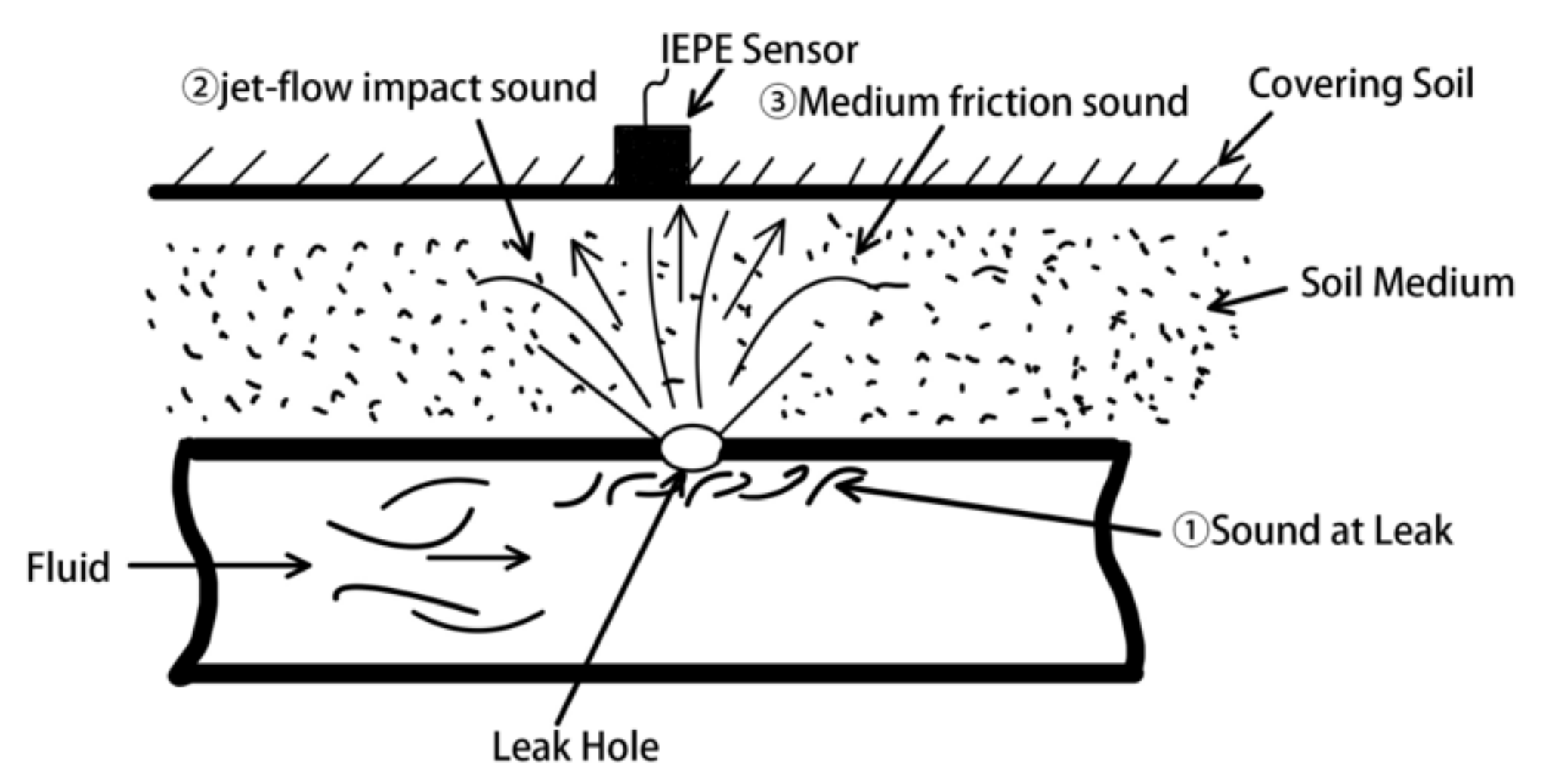
When there is leakage in a WDS, the high-pressure jet flow inside the pipe escapes through the leak and interacts with the pipe wall, producing vibration of different frequencies. According to the location of the vibration, sound origin can usually be divided into the following three types:
Acoustic emission signals at the leak: because the leakage is generally an elastic fluid, the leakage inside the pipe not only disorders the normal flow but also interacts with the pipe wall and spreads along the pipeline axis. The transmission distance and decay degree are generally related to the pressure, the pipe material, the pipe diameter, and the number of interfaces. The vibration can be detected at a distance from the leak at a valve, a hydrant, and a pipe.
The jet-flow impact sound refers to the sound of the high-pressure jet flow impacting the leaking wall and the covering medium of the pipe. The sound signal funnels to the ground and can be detected on the ground.
Friction sound of the physical medium: the water jet escaping from the pipe drives the surrounding medium particles to collide and rub against the pipe wall.
In the leak detection operation, an integrated electronics piezo-electric (IEPE) sensor with a magnetic base is usually employed to absorb the vibrations of the outer wall of the pipe, the fire hydrant, and the valves in the overhaul well, so as to collect the signals. Figure 1 illustrates the generation and collection of the acoustic emission signals of a pipeline leakage schematically.
The signals at the leak primarily comprise the air bubble sounds, turbulent sounds, and the pulse impacts of the turbulent adhesion layer.
3. Basic Characteristics of Acoustic Emission Signals
3.1. Power Spectrum
To accurately describe the statistical characteristics of a stationary random signal in the frequency domain, we set a power spectral density function defined as the Fourier transform of the autocorrelation function for the signal [6]
where is the power spectral density (PSD), denotes the autocorrelation, τ is the time step, and ω stands for the frequency.
The Wiener–Khinchin theorem describes the relationship between the power spectrum of a stationary random signal and its autocorrelation function [17].
The modern spectral estimation method requires a rank to establish a parametric model according to the estimation of the sample data and to solve the output of the parametric model so as to transform the power spectrum estimation into the problem of solving for the parametric model [18]. The autoregressive (AR) model is most commonly used for power spectrum estimation in modern methods since it is simply computed, and its parameters can be directly obtained through a set of linear equations. The AR model considers the random signal sequence a linear combination of its several past values and its present motivated values.
The power spectral density function of is defined as [6]:
where is the signal, denotes the power spectral density, is the number of sampling points, is the variance of Gaussian white noise, and is the parameter of the k-order AR model.
In general, the order selection of the AR model primarily depends on three criteria: the final prediction error criterion, the Akaike information criterion (AIC), and the discriminant autoregressive transmission function criterion [19]. In practice, selecting the order p of the autoregressive model determines the performance of the power spectrum estimation, so the reasonable choice of the order p is critical.
3.2. Spectral Roll-Off Rate
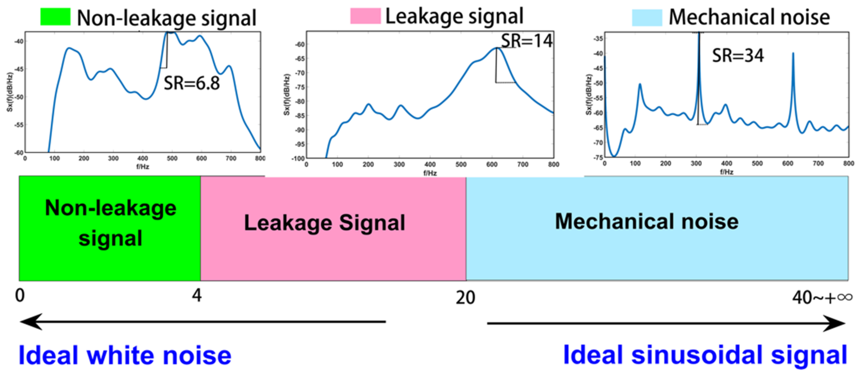
The spectral roll-off (SR) describes the descent rate of the spectrum. It is usually believed that the radiation noise of ships drops at 6 dB/time in high-frequency bands, but it differs for various noise origins. The main reason is the various degrees of cavitation, such as surface sailing merchant ships, underwater submarines, and torpedoes, the spectral roll-off rates of which are different.
The spectral roll-off rate is usually expressed as the average of the descent rate after the power maximum point, with an index in the dB/fold range, using the below equation [20]:
where represents the maximum power spectrum when the frequency equals F, and indicates the power spectrum value at n times beyond the frequency F.
The distribution of the spectral roll-off rates is determined by analyzing a large amount of data, as shown in Figure 2. Generally, the larger the roll-off rate of the signal, the higher the energy of the signal components, such as strong pulse signals and ideal sinusoidal signals. A lower spectral roll-off rate leads to a higher average energy of that component. According to the previous analysis, the spectral roll-off rate of the acoustic emission signals of the pipeline with a leakage is distributed in the range of 0–20 dB, while that of the acoustic emission signals of the pipeline without a leakage is closer to 0 dB.
3.3. Spectral Flatness
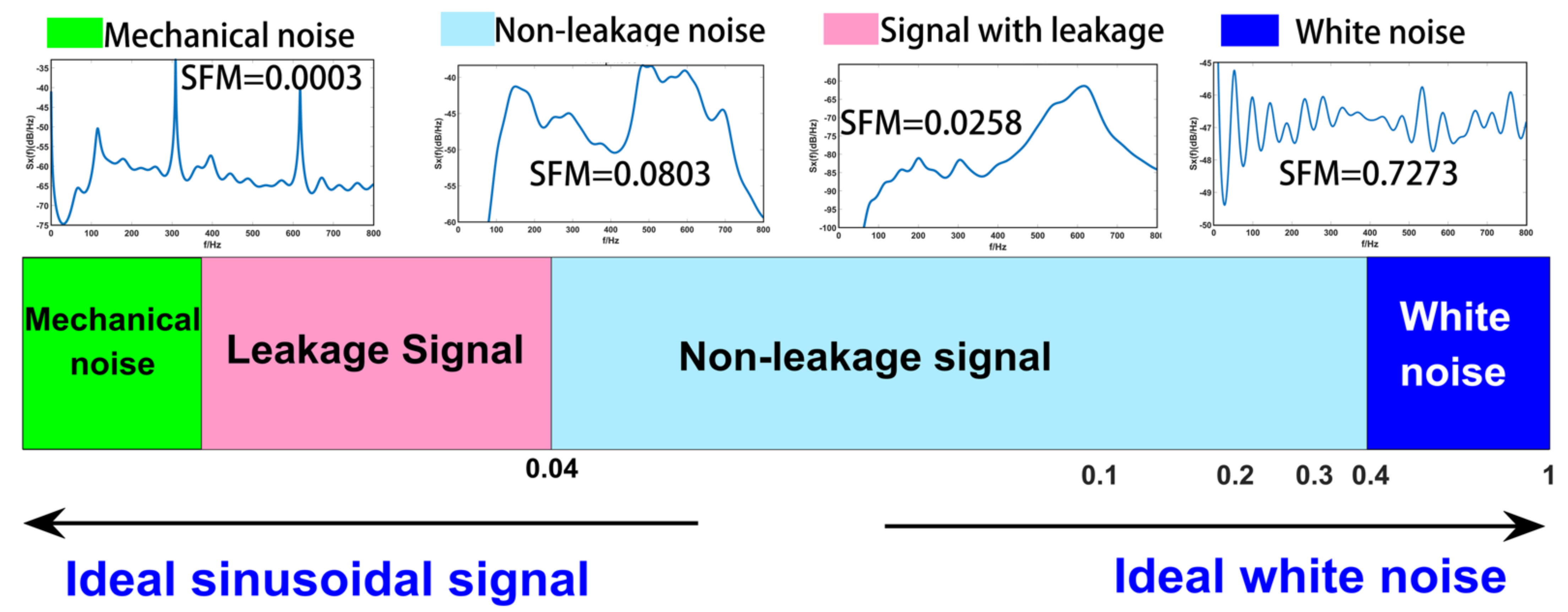
Spectral flatness measurement (SFM), defined as the ratio of the geometric mean (GM) of a spectrum to its arithmetic mean (AM), is utilized to quantify the flatness of the spectrum. An SFM closer to zero indicates that the signal is highly similar to the sinusoidal curve or that there is a meaningful signal. An SFM closer to 1 implies that the higher the SFM is, the lower the correlation of the signal becomes. An SFM equal to 1 denotes a white noise, no meaningful signal, or a meaningful signal submerged by the higher intensity of the white noise. The below formula calculates the spectral flatness [21]:
where GM represents the geometric mean of the spectrum, AM stands for the arithmetic mean of the spectrum, N indicates the length of the signal, and denotes the signal.
Figure 3 illustrates the definition and classification of spectral flatness.
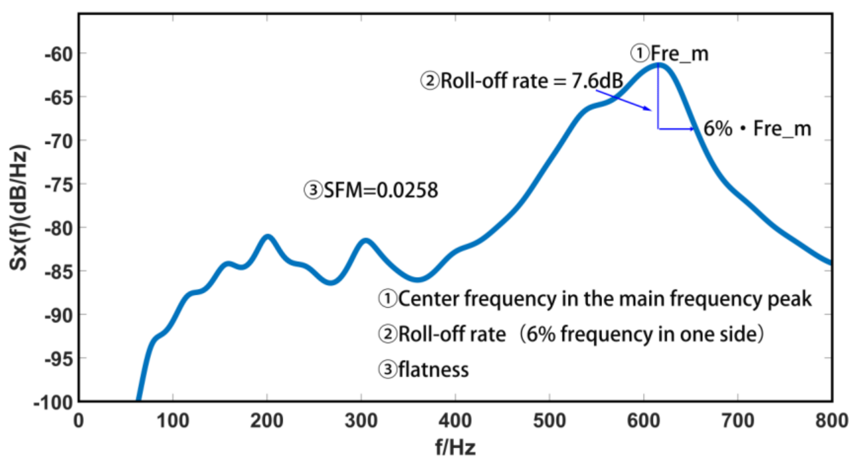
Figure 4 briefly presents the application of the central frequency peak, the spectral roll-off rate, and the spectral flatness in a specific example.
4. Analyzing the Frequency Characteristics of Acoustic Emission Signals Associated with Pipeline Leakage
4.1. Distribution of the Central Frequencies of the Power Spectrum
After processing and analyzing over 6800 signals collected in this paper, the power spectrum characteristics of the leak detection signals were as follows.
The acoustic emission signals of the WDS had an approximate “periodic” characteristic, so a “wide peak” characteristic is indicated in the power spectrogram.
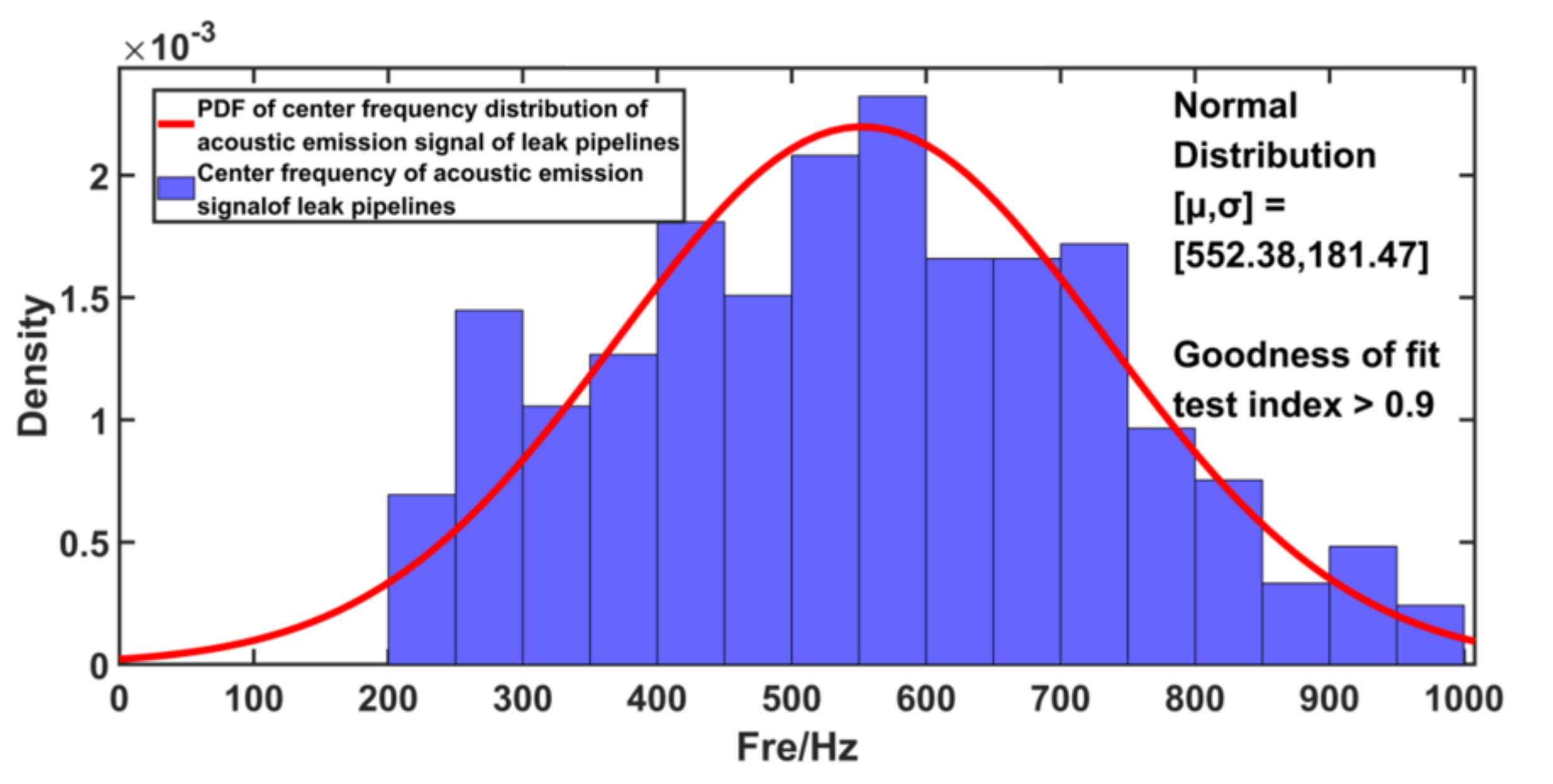
The frequency of the leak detection signals of the WDS mostly ranged from 200 to 800 Hz, and signals in the other frequency ranges were relatively rare. More than 3000 groups were marked as leakage among the signals collected in this paper. Figure 5 illustrates the distribution of the central frequencies of the acoustic signals of the water supply pipeline with a leakage. The dominant frequency distribution of the acoustic signals of the water distribution system with a leakage was evidently a normal distribution. After the analysis, the following distribution formula was obtained [22]:
where represents the probability distribution function (PDF), denotes the central frequency of the signal, σ indicates the standard deviation, and µ is the expectation.
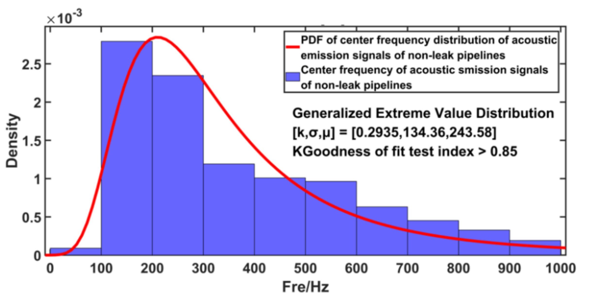
In contrast, the central frequencies of the acoustic signals of the WDS without a leakage follow a generalized extreme value distribution [23], different from that of pipelines with a leakage, as depicted in Figure 6,
where represents the PDF, and denotes the central frequencies of the acoustic signals of the WDS without a leakage.
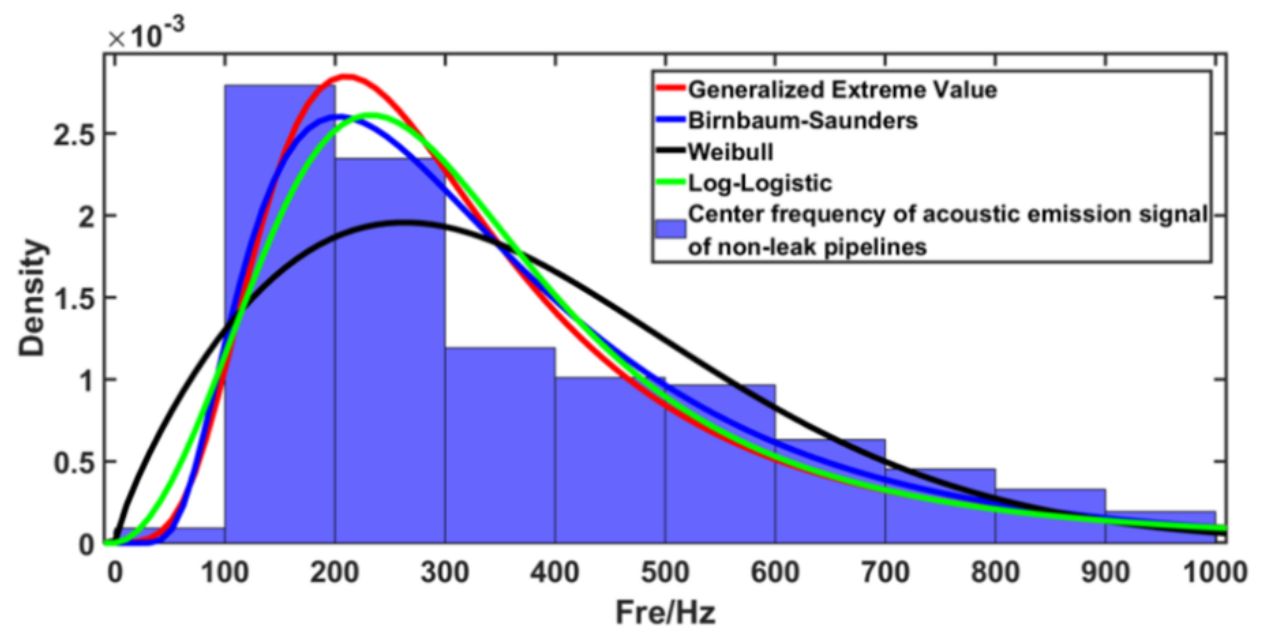
Comparing the standard distributions fitting the central frequencies of the acoustic emission signals of the pipeline without a leakage we obtained the generalized extreme value distribution, as depicted in Figure 7.
The power spectrum characteristics of some interference noise were similar to those of the signals of the WDS with a leakage, and it was challenging to distinguish them only by the central frequency characteristics. The power spectrum characteristics of the leak detection signals of the water distribution system play a vital role in determining whether a leakage occurs, but the power spectrum characteristics alone are not enough.
4.2. Distribution of Spectral Roll-Off Rates
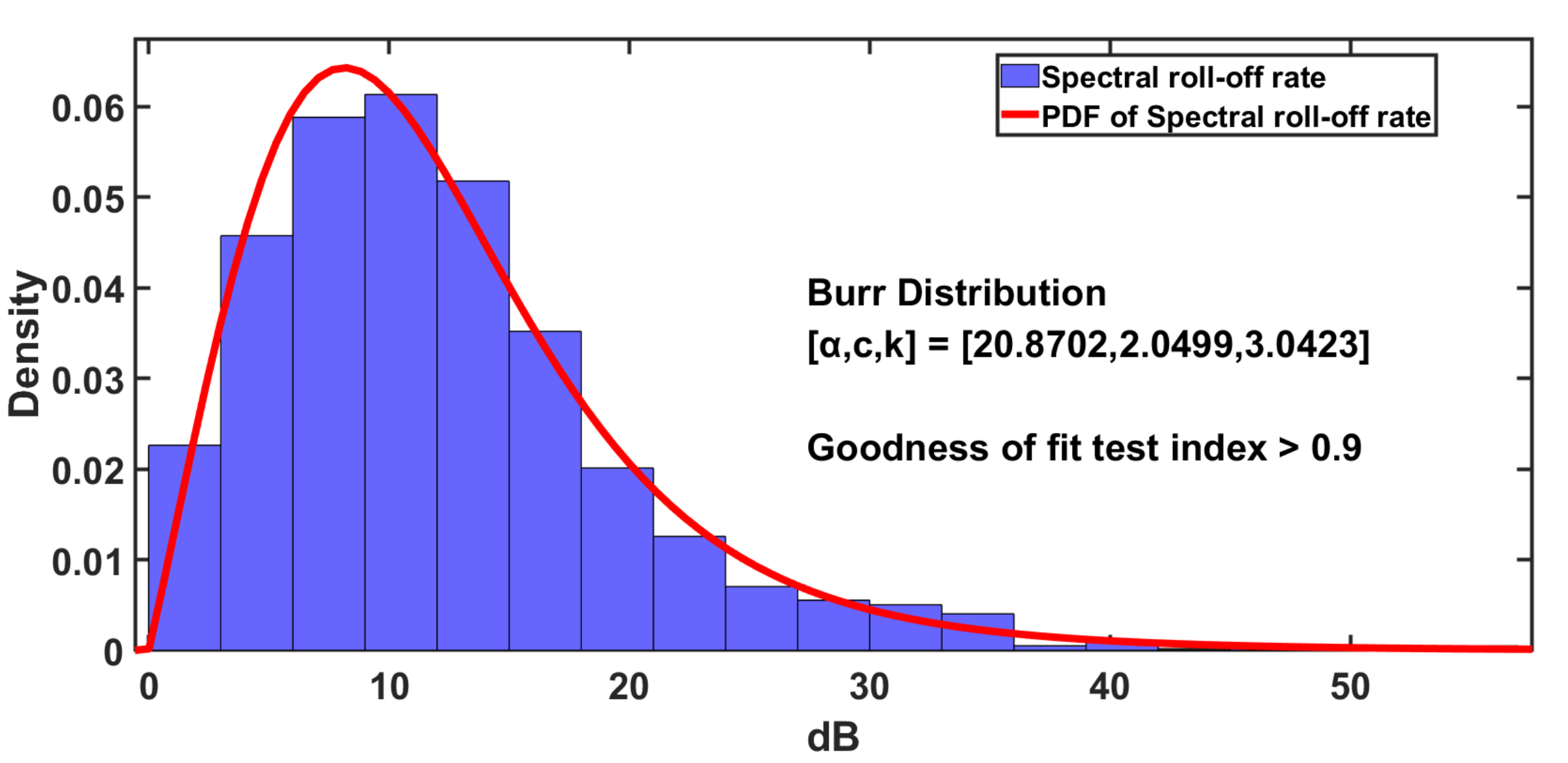
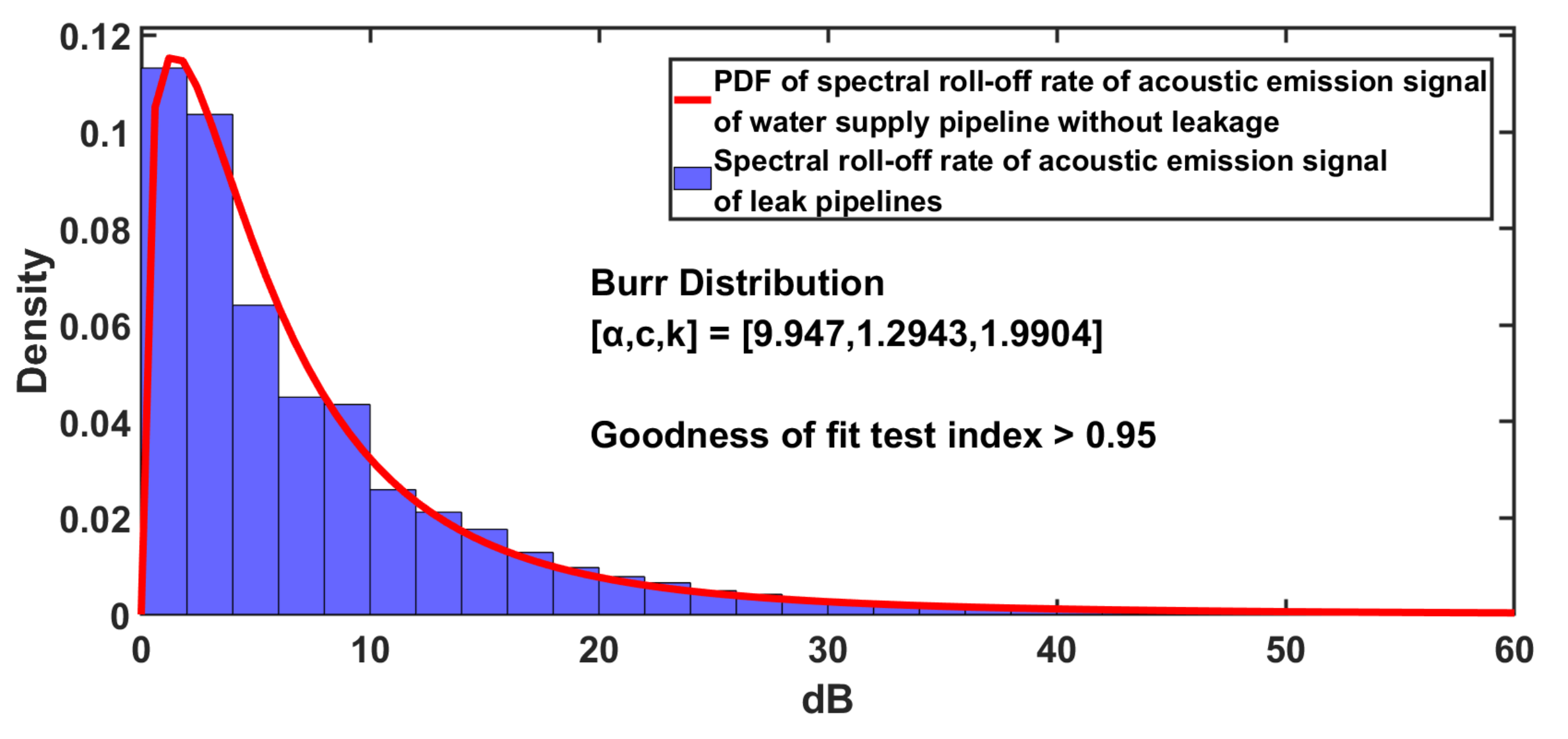
Similarly, the spectral roll-off rates of the signals collected in this work were analyzed from a statistical viewpoint, as illustrated in Figure 8. According to the spectral roll-off rate distribution, the peak of the leakage acoustic signals appeared mostly around 10 dB, while the ratio of the signals between 5 and 15 dB reached 57%. Further, the distribution of the nonleakage signals was closer to 0 dB. The spectral roll-off rates in the range of 0 to 5 dB accounted for 51% of the total rates, while those between 0 and 10 dB accounted for 75%. The distribution of the spectral roll-off rates of the signals showed a remarkable statistical feature, and the spectral roll-off rates of the leakage signals followed a three-parameter Burr distribution as follows [24]:
where represents the PDF, denotes the spectral roll-off rate, α indicates the shape parameter, c is the inequality parameter, and k stands for the scale parameter.
Figure 8 delineates the probability density function (PDF) of the spectral roll-off rates of the acoustic emission signals of pipelines with a leakage.
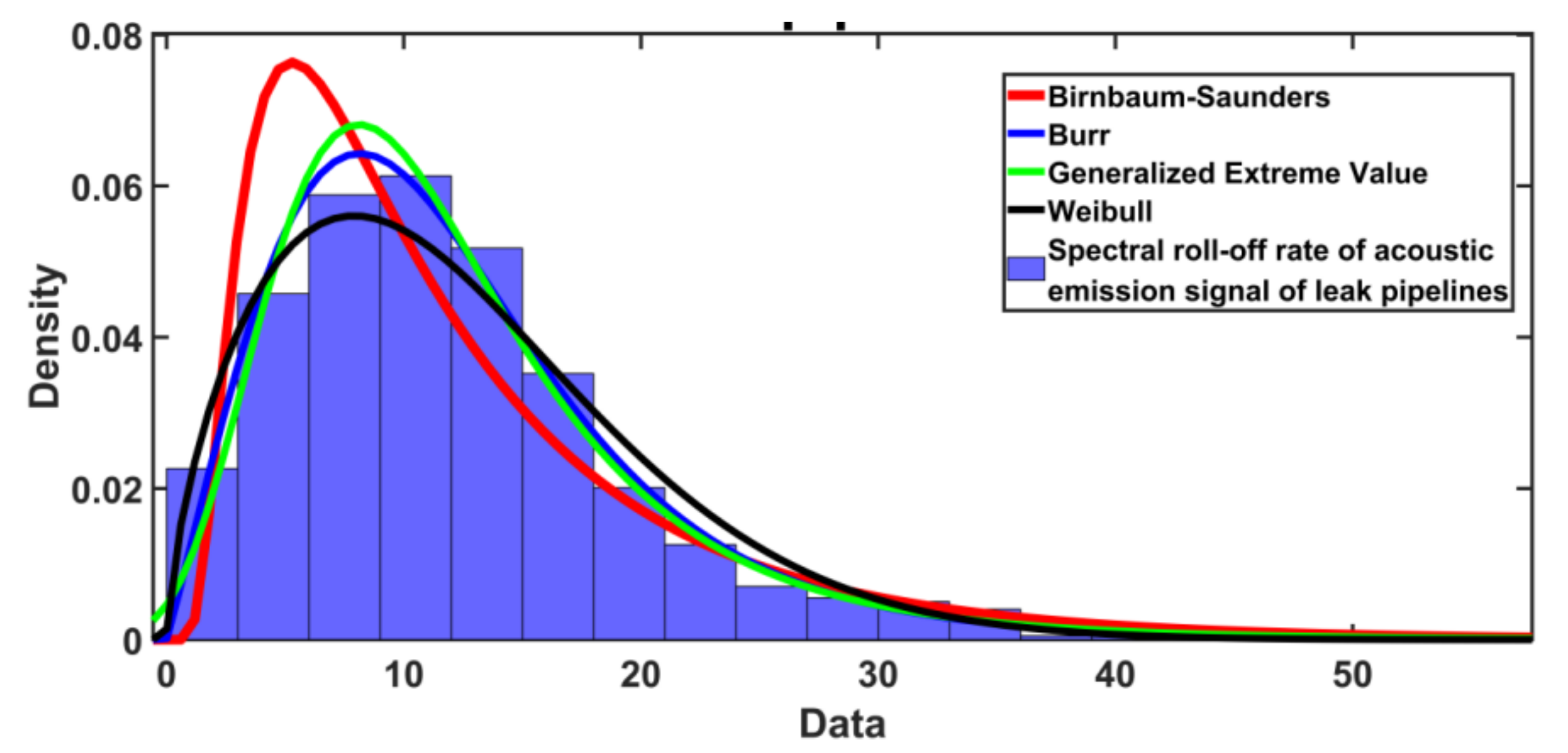
Comparing the standard distributions fitting the spectral roll-off rates of the acoustic emission signals of the pipelines with a leakage we obtained the Burr distribution, as shown in Figure 9.
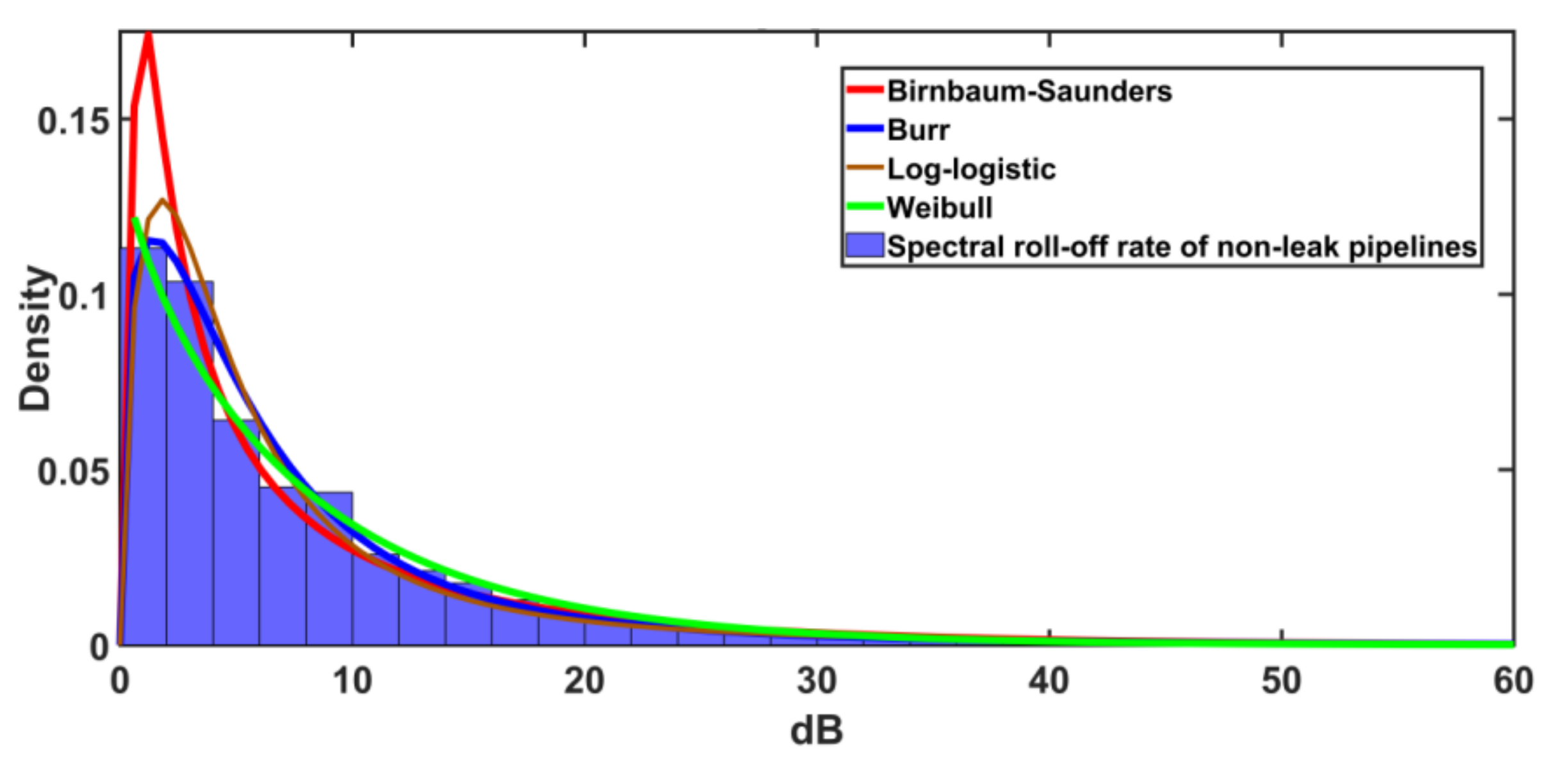
The data of the signals of the pipelines without a leakage also conformed to the three-parameter Burr distribution as follows [24], but the distribution was closer to 0 dB.
where represents the PDF, α indicates the shape parameter, c denotes the inequality parameter, and k stands for the scale parameter.
4.3. Distribution of the Spectral Flatness
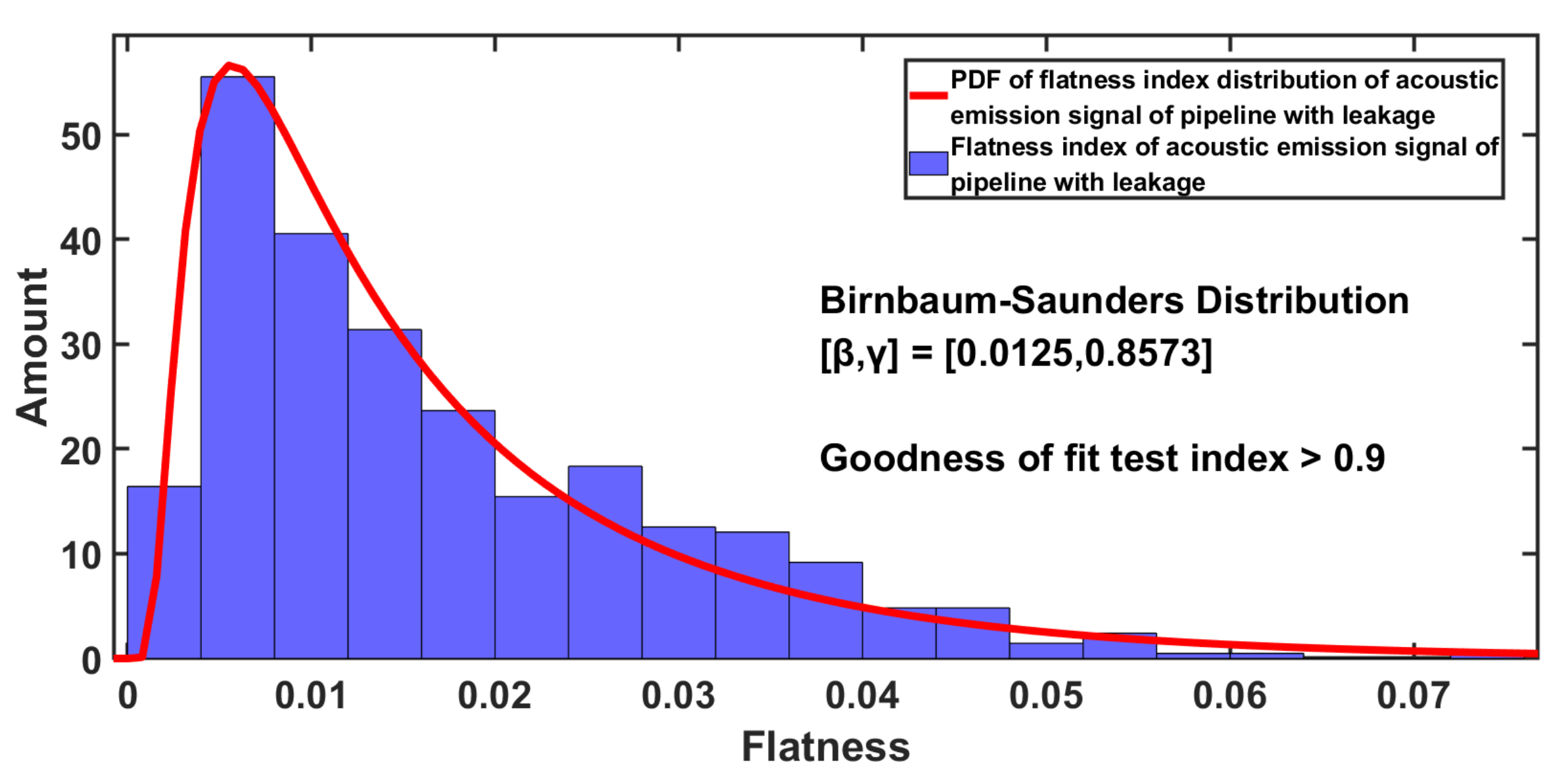
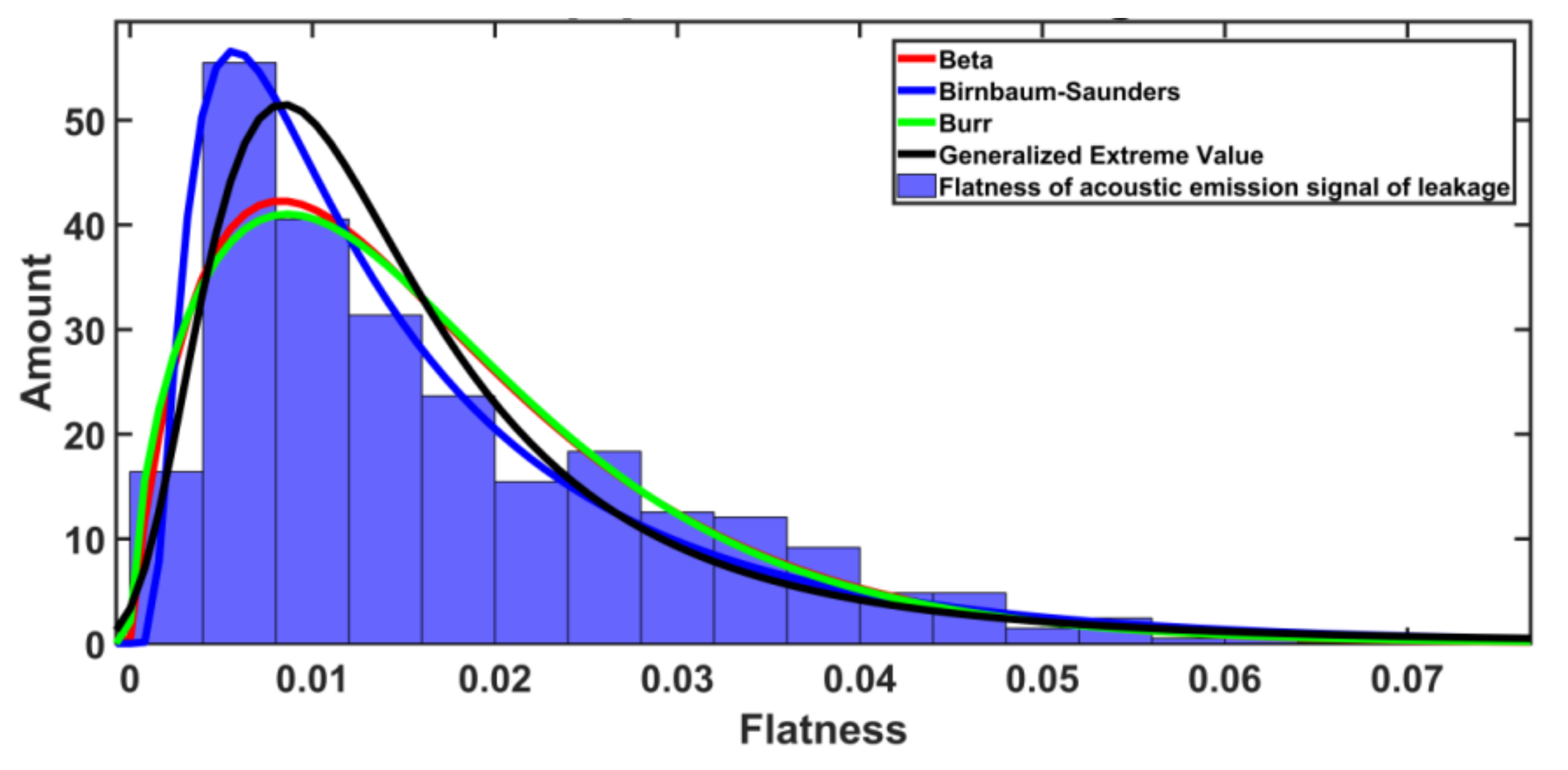
Likewise, the spectral flatness indicators of the leak detection signals were extracted and counted. Figure 12 show the distributions of the spectral flatness of the acoustic emission signals of water distribution systems with and without a leakage respectively. According to the histograms, the spectral flatness characteristics of the acoustic signals of the water distribution systems with and without a leakage were distributed in two distinct intervals. Overall, the spectral flatness of a leakage acoustic signal was less than that of a nonleakage acoustic signal, and 94% of the spectral flatness indicators of the leakage signals ranged from 0 to 0.04. In other words, only 6% of the indicators of the leakage signals were higher than 0.04, while 54% of the spectral flatness indicators of the nonleakage signals were beyond 0.04. Since the number of the leakage signals was 20% of the whole data set, a spectral flatness higher than 0.04 was about 98% likely to belong to a nonleakage signal. Even if the leakage and nonleakage signals were equal in number, a spectral flatness over 0.04 was about 93% likely to belong to a nonleakage signal. In practical leak detection, leakage signals are far fewer than nonleakage signals. Hence, spectral flatness can be used to effectively exclude nonleakage signals, and this indicator is of practical significance in leak detection operations.
Analyzing the data demonstrated that the spectral flatness distribution of the leakage signals conformed to the Birnbaum–Saunders distribution [25], as shown in Figure 12. The distribution equation is expressed as:
where represents the PDF, and β and γ are the parameters of the B–S distribution.
Comparing the standard distributions fitting the spectral flatness of the acoustic emission signals of the pipelines with leakage, we obtained the Birnbaum–Saunders distribution, as depicted in Figure 13.
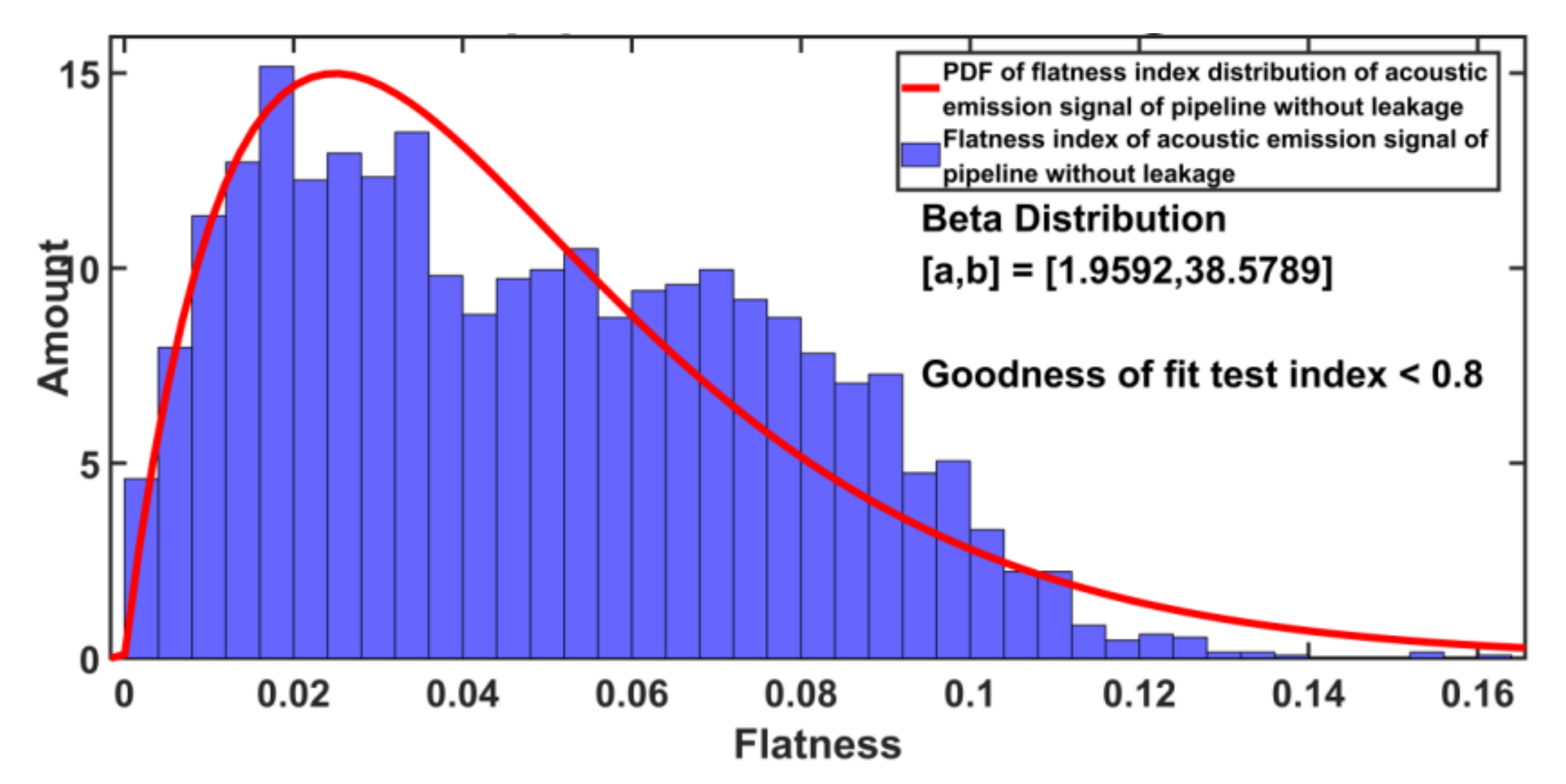
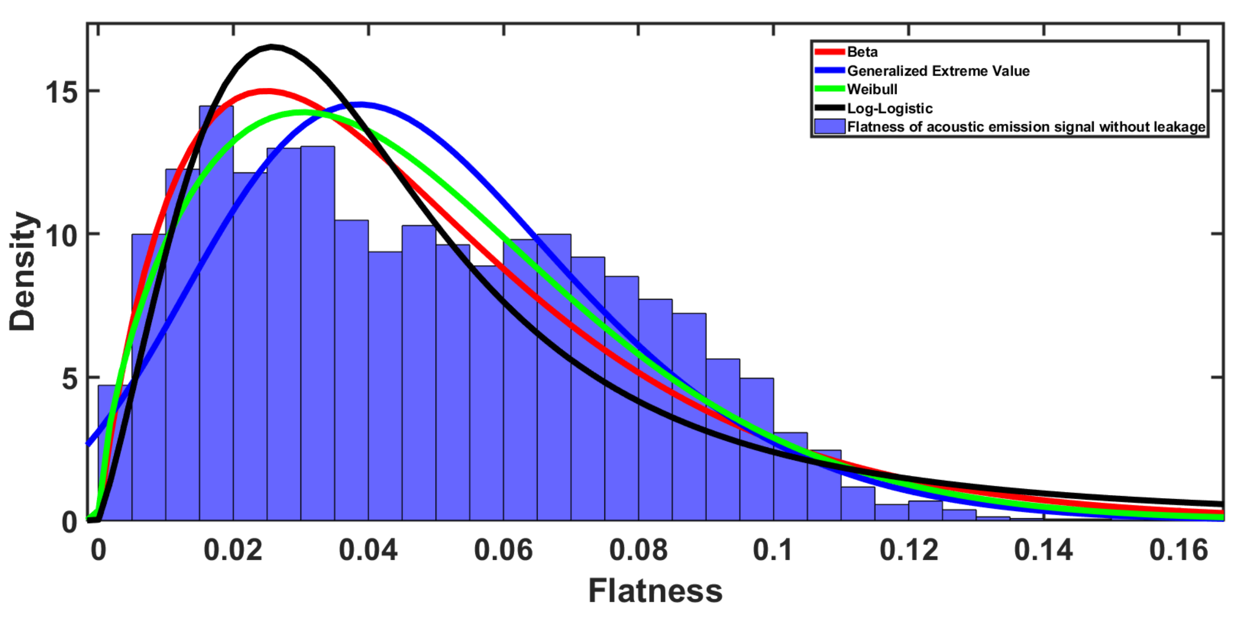
The formula for the spectral flatness distribution of the acoustic emission signals of the water distribution system without a leakage did not pass the goodness-of-fit test, and the standard statistical distributions did not reach a level of significance of 80%. Figure 14 and Figure 15 delineate the PDF obtained by fitting and the fitting process. The best fitting model obtained was as follows [26]:
where represents the PDF, a and b are the parameters of the Beta distribution, and B stands for the Beta distribution.
5. Performance of the Random Forest Classification Model
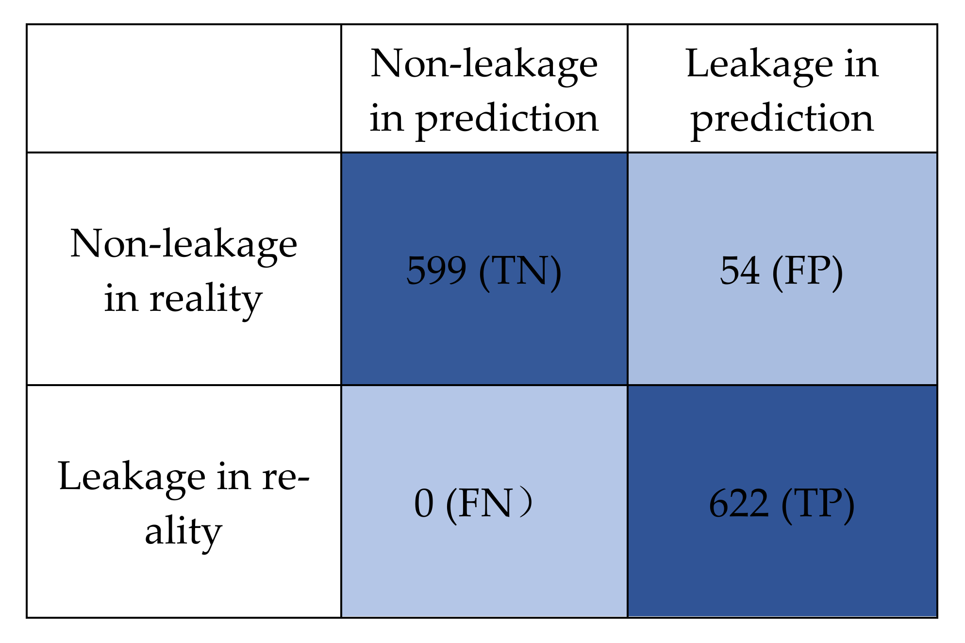
Random forest is used to distinguish signals in the presence or absence of a leakage from the detection signals. It is composed of many decision trees not related to each other. During the model running, each part will obtains classification results separately. The final result of the model is determined by the voting method. In this research, the depth of Random Forest was set to 50, and the number of trees of that was set to 280. The feature of {the central frequency peak, spectral roll-off rate, the spectral flatness} was set as the input data of the Random Forest model. In this task, the numbers of training and validation data were set to 80 and 20. There were 6380 input data, of which 3113 were leakage data, and 3272 were non-leakage data. The confusion matrix of the Random Forest model’s validation is shown in Figure 16.
The indicators in Table 1 can be used to evaluate the Random Forest model’s performance.
In general, a precision of 90% means a good performance model, and the random forest model showed a good overall classification accuracy of 92.01% for the leak detection task. The closer the F value is to 1, the better the robustness of the model. This model had an F1_score of 0.9584, higher than the general standard of 0.9. The recall rate of 100% and the false positive rate of 8.27% mean that the model found leakage signals well and the possibility of misjudgment of non-leakage signals was low. While improving the efficiency of leak detection, this model also reduces the ground loss of excavation caused by false positives.
6. Conclusions
This paper extracted the characteristics of leak detection signals and statistically summarized them in terms of central frequency, spectrum roll-off rate, and spectrum flatness.
The “wide peak” characteristic appeared on the power spectrum, and the central frequencies of the signals ranged from 200 to 800 Hz, approximately conforming to the normal distribution.
In a unilateral frequency range of 6%, the distribution of the spectral roll-off rates of the acoustic emission signals of the pipelines with a leakage had a significant statistical characteristic and conformed to the Burr distribution.
The distribution of the spectral flatness of the acoustic signals complied with the Birnbaum–Saunders distribution and could be used to exclude the nonleakage signals in leak detection.
The distribution of the acoustic emission signals of leak detection in water distribution systems has a significant statistical characteristic, which is of practical importance for leak detection operations. The probability distribution function of the individual probability can be used to judge the probability of leakage signals. In this research, the Random Forest model was used to classify the leakage detection signals, with a recall rate of 100% and a false positive rate of 8.27%. The automation of the leak detection of WDSs based on intelligent methods has changed the long-term status of leak detection operations relying on manual work.
Author Contributions
Conceptualization, W.C. and Y.S.; Methodology, Y.S.; Software, Y.S.; Validation, Y.S.; Formal Analysis, Y.S.; Investigation, Y.S.; Resources, W.C.; Data Curation, W.C.; Writing—Original Draft Preparation, Y.S.; Writing—Review & Editing, W.C. All authors have read and agreed to the published version of the manuscript.
Funding
This study was financially supported by the Zhejiang Key Research and Development Program (2021C03017).
Data Availability Statement
Not applicable.
Conflicts of Interest
The authors declare no conflict of interest.
References
- Muntakim, A.H.; Dhar, A.S.; Dey, R. Interpretation of Acoustic Field Data for Leak Detection in Ductile Iron and Copper Water-Distribution Pipes. J. Pipeline Syst. Eng. Pract. 2017, 8, 05017001. [Google Scholar] [CrossRef]
- Sousa, E.O.; Cruz, S.L.; Pereira, J.A.F.R. Monitoring Pipelines Through Acoustic Method. In Proceedings of the 10th International Symposium on Process Systems Engineering, Salvador-Bahia, Brazil, 16–20 August 2009; Volume 27, pp. 1509–1514. [Google Scholar]
- Meng, L.; Yuxing, L.; Wuchang, W.; Juntao, F. Experimental study on leak detection and location for gas pipeline based on acoustic method. J. Loss Prev. Process. Ind. 2012, 25, 90–102. [Google Scholar] [CrossRef]
- Mahmutoglu, Y.; Turk, K. Remote leak hole localization for underwater natural gas pipelines. In Proceedings of the International Conference on Telecommunications & Signal Processing, Barcelona, Spain, 5–7 July 2017; pp. 528–531. [Google Scholar]
- Wen, Y.; Zhang, X.; Wen, J.; Zhen, J.; Wang, K. Identification of water pipeline leakage based on acoustic signal frequency distribution and complexity. Yi Qi Yi Biao Xue Bao/Chin. J. Entific Instrum. 2014, 35, 1223–1229. [Google Scholar]
- Zhang, J.L.; Guo, W.X. Study on the Characteristics of the Leakage Acoustic Emission in Cast Iron Pipe by Experiment. In Proceedings of the 2011 First International Conference on Instrumentation, Measurement, Computer, Communication and Control, Beijing, China, 21–23 October 2011. [Google Scholar]
- Ni, L.; Jiang, J.; Pan, Y.; Wang, Z. Leak location of pipelines based on characteristic entropy. J. Loss Prev. Process Ind. 2014, 30, 24–36. [Google Scholar] [CrossRef]
- Vracar, M.; Kovacevic, N. Vibration of the vessel and bispectrum of hydroacoustic noise. Facta Univ.-Ser. Phys. Chem. Technol. 2009, 7, 45–60. [Google Scholar] [CrossRef]
- Luo, J.; Ushijima, T.; Kitoh, O.; Lu, Z.; Liu, Y. Lagrangian dispersion in turbulent channel flow and its relationship to Eulerian statistics. Int. J. Heat Fluid Flow 2007, 28, 871–881. [Google Scholar] [CrossRef]
- Tu, L.T.N.; Kim, J.-M. Discriminative feature analysis based on the crossing level for leakage classification in water pipelines. J. Acoust. Soc. Am. 2019, 145, EL611–EL617. [Google Scholar] [CrossRef] [Green Version]
- Mounce, S.; Husband, S.; Furnass, W.; Boxall, J. Multivariate data mining for estimating the rate of discoloration material accumulation in drinking water systems. Procedia Eng. 2014, 89, 173–180. [Google Scholar] [CrossRef] [Green Version]
- Li, S.; Wen, Y.; Li, P.; Yang, J.; Dong, X.; Mu, Y. Leak location in gas pipelines using cross-time–frequency spectrum of leakage-induced acoustic vibrations. J. Sound Vib. 2014, 333, 3889–3903. [Google Scholar] [CrossRef]
- Hunaidi, O.; Chu, W.; Wang, A.; Wei, G. Detecting leaks in plastic pipes. J.-Am. Water Work. Assoc. 2000, 92, 82–94. [Google Scholar] [CrossRef] [Green Version]
- Muggleton, J.M.; Brennan, M.J. Leak noise propagation and attenuation in submerged plastic water pipes. J. Sound Vib. 2004, 278, 527–537. [Google Scholar] [CrossRef]
- Brennan, M.J.; Karimi, M.; Muggleton, J.M.; Almeida, F.C.L.; de Lima, F.K.; Ayala, P.C.; Obata, D.; Paschoalini, A.T.; Kessissoglou, N. On the effects of soil properties on leak noise propagation in plastic water distribution pipes. J. Sound Vib. 2018, 427, 120–133. [Google Scholar] [CrossRef] [Green Version]
- Miller, R.K.; Pollock, A.A.; Finkel, P.; Watts, D.J.; Carlyle, J.M.; Tafuri, A.N.; Yezzi, J.J. The development of acoustic emission for leak detection and location in liquid-filled, buried pipelines. Acoust. Emiss. Stand. Technol. Update 1999, 1353, 67–78. [Google Scholar] [CrossRef]
- Lyamshev, L.M. Radiation acoustics. Sov. Phys. Uspekhi 1992, 35, 276. [Google Scholar] [CrossRef]
- Waele, S.D.; Broersen, P.M. Order selection for vector autoregressive models. IEEE Trans. Signal Process. 2003, 51, 427–433. [Google Scholar] [CrossRef]
- Levkovskii, Y.L. Effect of diffusion on sound radiation from a cavitation void. Sov. Phys. Acoust.-USSR 1969, 14, 470. [Google Scholar]
- Lalitha, S.; Mudupu, A.; Nandyala, B.V.; Munagala, R. Speech emotion recognition using DWT. In Proceedings of the 2015 IEEE International Conference on Computational Intelligence and Computing Research (ICCIC), Madurai, India, 10–12 December 2015; pp. 1–4. [Google Scholar]
- Herre, J.; Allamanche, E.; Hellmuth, O. Robust matching of audio signals using spectral flatness features. In Proceedings of the 2001 IEEE Workshop on the Applications of Signal Processing to Audio and Acoustics (Cat. No.01TH8575), New Platz, NY, USA, 24 October 2001. [Google Scholar]
- Roy, D. The discrete normal distribution. Commun. Stat.-Theory Methods 2003, 32, 1871–1883. [Google Scholar] [CrossRef]
- Bali, T.G. The generalized extreme value distribution. Econ. Lett. 2003, 79, 423–427. [Google Scholar] [CrossRef]
- Tadikamalla, P.R. A look at the Burr and related distributions. Int. Stat. Rev./Rev. Int. Stat. 1980, 48, 337–344. [Google Scholar] [CrossRef] [Green Version]
- Rieck, J.R.; Nedelman, J.R. A log-linear model for the birnbaum—Saunders distribution. Technometrics 1991, 33, 51–60. [Google Scholar]
- McDonald, J.B.; Xu, Y.J. A generalization of the beta distribution with applications. J. Econom. 1995, 66, 133–152. [Google Scholar] [CrossRef]
Figure 1.
Schematic of the generation of acoustic emission signals from a pipeline leakage.

Figure 2.
Classification standard for the roll-off rate of leakage detection.

Figure 3.
Classification standard for the spectral flatness of leakage detection.

Figure 4.
Application of the frequency characteristic parameters in a specific example.

Figure 5.
Distribution of the central frequencies of the acoustic signals of the water supply pipeline with a leakage.
Figure 5.
Distribution of the central frequencies of the acoustic signals of the water supply pipeline with a leakage.

Figure 6.
Distribution of the central frequencies of the acoustic signals of the water supply pipeline without a leakage.
Figure 6.
Distribution of the central frequencies of the acoustic signals of the water supply pipeline without a leakage.

Figure 7.
Comparison of the distributions fitting the central frequencies of the acoustic emission signals of the pipeline without a leakage.
Figure 7.
Comparison of the distributions fitting the central frequencies of the acoustic emission signals of the pipeline without a leakage.

Figure 8.
Distribution of the roll-off rates of the acoustic emission signals of pipelines with a leakage.
Figure 8.
Distribution of the roll-off rates of the acoustic emission signals of pipelines with a leakage.

Figure 9.
Comparison of the distributions fitting the spectral roll-off rates of the acoustic emission signals of the pipelines with leakage.
Figure 9.
Comparison of the distributions fitting the spectral roll-off rates of the acoustic emission signals of the pipelines with leakage.

Figure 10.
Distribution of the spectral roll-off rates of the acoustic emission signals of pipelines without a leakage.
Figure 10.
Distribution of the spectral roll-off rates of the acoustic emission signals of pipelines without a leakage.

Figure 11.
Comparison of the distributions fitting the spectral roll-off rates of the acoustic emission signals of pipelines without a leakage.
Figure 11.
Comparison of the distributions fitting the spectral roll-off rates of the acoustic emission signals of pipelines without a leakage.

Figure 12.
Distribution of the spectral flatness of the acoustic emission signals of WDSs with a leakage.
Figure 12.
Distribution of the spectral flatness of the acoustic emission signals of WDSs with a leakage.

Figure 13.
Comparison of the distributions fitting the spectral flatness of the acoustic emission signals of WDSs with a leakage.
Figure 13.
Comparison of the distributions fitting the spectral flatness of the acoustic emission signals of WDSs with a leakage.

Figure 14.
Distribution of the spectral flatness of the acoustic emission signals of WDSs without a leakage.
Figure 14.
Distribution of the spectral flatness of the acoustic emission signals of WDSs without a leakage.

Figure 15.
Comparison of the distributions fitting the spectral flatness of the acoustic emission signals of WDSs without a leakage.
Figure 15.
Comparison of the distributions fitting the spectral flatness of the acoustic emission signals of WDSs without a leakage.

Figure 16.
Confusion matrix of the validation of the Random Forest Model.


Table 1.
Indicators to evaluate the Random Forest model.
| Name | Meaning | Value |
|---|---|---|
| TN | Non-leakage in reality and in prediction | 599 |
| FP | Non-leakage in reality but leakage in prediction | 54 |
| FN | Leakage in reality but non-leakage in prediction | 0 |
| TP | Leakage in reality and in prediction | 622 |
| Precision | 92.01% | |
| Training accuracy | in training | 99.82% |
| Validation accuracy | in validation | 95.27% |
| Recall rate | 100% | |
| F1_score | 0.9584 | |
| False Positive Rate | 8.27% |
Publisher’s Note: MDPI stays neutral with regard to jurisdictional claims in published maps and institutional affiliations. |
© 2022 by the authors. Licensee MDPI, Basel, Switzerland. This article is an open access article distributed under the terms and conditions of the Creative Commons Attribution (CC BY) license (https://creativecommons.org/licenses/by/4.0/).
Share and Cite
MDPI and ACS Style
Cheng, W.; Shen, Y. Frequency Characteristic Analysis of Acoustic Emission Signals of Pipeline Leakage. Water 2022, 14, 3992. https://doi.org/10.3390/w14243992
AMA Style
Cheng W, Shen Y. Frequency Characteristic Analysis of Acoustic Emission Signals of Pipeline Leakage. Water. 2022; 14(24):3992. https://doi.org/10.3390/w14243992
Chicago/Turabian StyleCheng, Weiping, and Yongxin Shen. 2022. "Frequency Characteristic Analysis of Acoustic Emission Signals of Pipeline Leakage" Water 14, no. 24: 3992. https://doi.org/10.3390/w14243992
Note that from the first issue of 2016, this journal uses article numbers instead of page numbers. See further details here.