
Contrast Analysis of Flow-Discharge Measurement Methods in a Wide–Shallow River during Ice Periods


1
State Key Laboratory of Simulation and Regulation of Water Cycle in River Basin, China Institute of Water Resources and Hydropower Research, Beijing 100038, China
2
Department of Hydraulic Engineering, Tsinghua University, Beijing 100084, China
*
Author to whom correspondence should be addressed.
Water 2022, 14(24), 3996; https://doi.org/10.3390/w14243996
Submission received: 18 October 2022
/
Revised: 1 December 2022
/
Accepted: 3 December 2022
/
Published: 7 December 2022
(This article belongs to the Special Issue Advanced Turbulence Measurements and Simulations in River Flow Research: From Experimental Flume- and Field- Scale Experiments to Computational Fluid Dynamics (CFD))
Abstract
:The discharge of natural rivers is one of the important hydrological factors that are considered when responding to ice-flood disasters during ice periods. Traditionally, holes need to be dug along the cross-section on the ice cover to gauge velocity distributions along the flow depth at each hole, and to calculate the cross-sectional flow discharge by integrating velocity profiles over the entire area. This method is time consuming, costly, and inefficient. The discharge measurement can be improved using the sectional flow-depth distribution and stream-tube methods. However, the selection of both the depth-averaged–velocity-estimation method and the typical survey-point position in the cross-section affects the estimation accuracy. This study first compared the estimation methods of the depth-averaged velocity, such as the one-, two-, three-, and six-point methods, and their estimation accuracy. Furthermore, the variations in relative-unit discharge distributions in common channels with cross-sectional topographies were analyzed, and the effects of the cross-section characteristic coefficient and typical survey-point position on the flow-discharge estimation accuracy were compared. The results show that the average errors of the depth-averaged velocity estimated by the one-point method at 0.5H, new three-point method, and six-point method were 1.96%, 1.22%, and 0.45%, respectively. The new three-point method is recommended if measurement workload and accuracy are key considerations. The cross-section characteristic coefficient is considered to be 0.5 and 0.25 for the natural river and artificial channel, respectively, and the maximum-flow-depth position in the mainstream area of the cross-section is selected as the typical survey-point position. Thus, the flow-discharge estimation accuracy can be improved. In conclusion, this study provides an improved stream-tube method for the measurement of flow discharge and velocity distribution in ice periods, which can be used as a reference during practical applications.
1. Introduction
In the northern hemisphere, approximately 60% of rivers are significantly impacted by the seasonal effects of river ice [1]. Under-ice discharge is an important hydrological element during ice periods, which is of immense significance for predicting potential ice disasters, such as ice jams, during the ice-covered period, as well as for river management, directing, and decision-making linked to ice-disaster prevention [2,3].
There have been many studies on the measurement of flow discharge in ice periods, mainly focused on theoretical model analyses and conventional measurements. Healy and Hicks [4] explored the feasibility of using the exponential-velocity method in winter flow measurements based on data collected from eight hydrographic stations. They concluded that a specific relationship exists between exponential and average velocity, and the overall cross-sectional flow discharge can be determined from the velocity measured at selected cross-sectional points. Based on the three-dimensional Reynolds-averaged Navier–Stokes equations, Yang [5] obtained a quasi-two-dimensional model of the lateral-velocity distribution applicable to both uniform and non-uniform flows, which can effectively estimate the lateral-velocity distribution and the total-flow discharge in ice-covered channels. Mitchel et al. [6] and Kimiaghalam et al. [7] analyzed the influence of ice cover on flow discharge and velocity distribution through experimentation and showed that the presence of partial ice cover significantly increased channel-flow velocity and boundary-shear stress. Additionally, it changed the flow structure when compared to open channels, which is consistent with previous studies [8,9,10,11,12]. This augments the existing knowledge on flow characteristics in covered channels and provides a theoretical basis for its design and modeling. The United States Geological Survey (USGS) conducted a proof-of-concept study in the south of Minturn, Colorado (CO), USA, and developed an alternate method for computing under-ice discharge based on hydroacoustics and the Probability Concept [13]. Uncertainty in approaches to advanced computing plays an important role in the monitoring and protection of water resources [14,15,16], and this method poses major advantages for ecohydraulic modeling [14] and the indirect estimation of wind–wave heights [15]. Further study is required for future applications.
In terms of measurement methods, Walker [17] contrastingly analyzed the accuracy of various flow-discharge estimation methods such as the discharge-ratio during ice and non-ice periods, hydrographic-and-climatic comparison, adjusted-rating-curve considering the roughness of the ice cover, and index-velocity and the uniform-flow techniques. The results showed that different measurement methods have a large bias and uncertainty, and a more accurate flow-discharge measurement still relies on the cross-sectional–multi-point integration method. However, the method requires digging multiple holes on the ice cover along its cross-section, to gauge velocity distributions along the flow depth and to calculate the cross-sectional flow discharge by integrating velocity profiles over the entire area, which is time consuming, labor intensive, and not conducive to field measurement [4]. To improve the efficiency of flow-discharge measurements during ice periods, Shen and Ackermann [18] proposed the stream-tube method. This method ignores the transverse circulation and frictional forces on the interface and presents a transverse-distribution formula of unit discharge from ice-covered channels. Based on this, Pan [19] proposed a flow-discharge measurement method during ice periods that combines the stream-tube and Einstein’s splitting method for cross-sections, which only requires the vertical-flow–velocity-distribution measurement at one typical survey-point position and the distribution of flow depth along the cross-section. The cross-sectional characteristic coefficient and topographic data are then combined to derive the total discharge in the section, thus reducing the measurement workload of velocity distribution at multiple survey-point positions, which is a promising flow-discharge estimation method.
The above research shows that for both the multi-point integration or the stream-tube method, the vertical-flow-velocity distribution or depth-averaged velocity at a certain position must be obtained. In this regard, Lau [20] and Mao et al. [21] calculated the velocity distribution of river flow based on different boundary roughness conditions using the k–ε turbulence model, and theoretically proved that the average of the velocities at 0.2H (0.2 times the effective depth) and 0.8H (0.8 times the effective depth) was equal to the overall mean velocity of the frozen river. Although the two-dimensional k–ε turbulence model can be used to calculate the channel-flow velocity, this requires many empirical constants and is time consuming; therefore, Shiono and Knight [22] proposed an improved analytical model applicable to uniform turbulence in compound channels, which can derive the channel depth-averaged velocity and the lateral distribution of the boundary-shear stress relatively easily. Based on the research of Odgaard [23] on open-channel flow, Tsai [24] proposed the two-power-law expressions of vertical velocity under ice cover through theoretical deduction and verified these by flume experiments. This approach is advantageous because it expresses the vertical velocity using a single continuous curve, which is convenient to use when analyzing the influence of ice cover and riverbed roughness on vertical-velocity profiles. Determination of the formula parameters by measuring the velocity on a single measuring point provides satisfactory results, and this theoretical method has also been widely used. In practice, to simplify the measurement of velocity under ice cover, the vertical depth-averaged velocity can be obtained by point-velocity measurements via the one-, two-, three-, and six-point methods. For example, the USGS measured 2300 vertical-velocity profiles between 1988 and 1989, and the Canadian Water Resources Survey (WSC) measured 1800 vertical-velocity profiles between 1989 and 1991, both of which contributed to a joint database that confirmed the feasibility of the two current flow-measurement methods: the one-point method at 0.5H or 0.6H and the two-point method at 0.2H and 0.8H [25]. Later, Walker et al. [26] and Teal et al. [27] proposed that the one-point method at 0.5H, the two-point method at 0.4H and 0.8H, and the two-point method at 0.2H and 0.8H, also showed good estimation accuracies by analyzing the measured data at different measuring stations during ice periods. Recently, Shan et al. [28] confirmed the feasibility of describing the velocity distribution under ice cover according to the second log-wake law by analyzing the influence of ice covers on flow velocity and proposed a new three-point method based on this law. To represent the vertical-average velocity, the new method selects the point velocity at 0.2H, 0.5H, and 0.8H. “Liquid-flow measurement in open channels—Flow measurements under-ice conditions” is proposed in ISO 9196 [29] and considers the flow depth as the basis for method selection during ice-covered periods, and multiple measurement points need to be arranged when the flow depth is relatively large. When the measurement conditions cannot satisfy the required number of measuring points, the estimation accuracy of each method must be considered when determining a more appropriate flow-measurement scheme. Although the above studies are based on extensive measured data, they draw inconsistent conclusions in simplifying the measurement of depth-averaged velocity under ice cover.
The stream-tube method is efficient, time-saving, and accurate, decreasing the gauging risk of operations. However, the existing stream-tube method still has some limitations: (i) the estimation methods of depth-averaged velocity of a single survey point only provide the two-point method at 0.2H and 0.8H; (ii) the proposed position of the survey point is arbitrary, but the selection of both the depth-averaged–velocity-estimation method and the typical survey-point position in the cross-section affects the estimation accuracy.
Thus, the purpose of this study was to: (i) compare the estimation methods of depth-averaged velocity, such as the one-, two-, three-, and six-point methods, and their estimation accuracies; (ii) analyze the variation in the relative-unit discharge distributions of common river cross-sections with a cross-sectional topography; and (iii) determine the influence of cross-section characteristic coefficients and typical survey-point positions on the accuracy of flow-discharge estimation by the stream-tube method. Ultimately, we propose recommended estimation methods of the depth-averaged velocity, considering the measurement workload and accuracy factors. Additionally, this study aims to improve the stream-tube method and provide a reference for the flow-discharge measurements during ice periods.
2. Methods and Applications
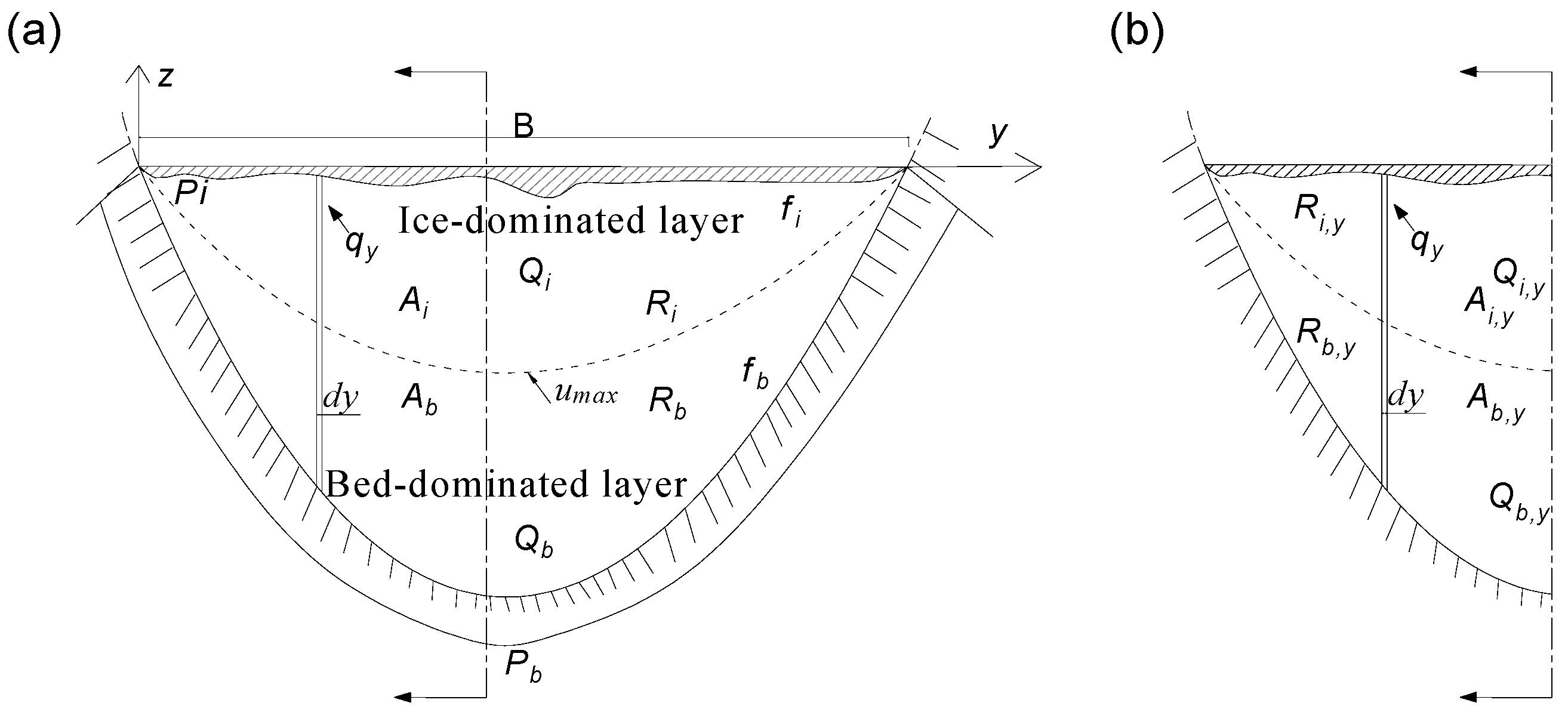
2.1. Stream-Tube Method
To obtain the cross-sectional velocity distribution and total discharge using the stream-tube method, only the single line depth-averaged velocity measurement is required at a typical position, along with the cross-sectional topographic data. The method is based on Einstein’s splitting method for cross-sections [30]. As shown in Figure 1a, the isoline of the maximum velocity divides the flow profile into two layers: the bed- and ice-dominated layers.
The partial cross-sectional discharge Qy along the cross-section from the starting point to point y at any position can be written as:
where subscript b is the parameter related to the riverbed, subscript i is the parameter related to the ice cover, subscript y indicates the hydraulic parameters of the partial sections, when y is considered as the entire section width, and Qy is equal to the overall cross-sectional flow-discharge Q, as shown in Figure 1a,b.
The ratio of the partial flow in section Qy to the overall flow in the section can be expressed by Equation (2), proposed by Shen and Ackermann [18]:
where A and R are the total area and hydraulic radius of the cross-section, respectively. The subscript y is consistent with the definition above.
The coordinate system used in this study is shown in Figure 1a. The unit discharge distribution along the y direction is expressed as:
The relative value of the unit discharge at any point k is expressed as [19]:
where point k represents any position on the cross-section, is the relative-unit discharge at point k, and α is the characteristic coefficient of the cross-section to be calibrated, which is related to the survey-point position and is a function of the ratio of the wet perimeter and hydraulic radius between the partial and the entire cross-section, and the ratio of the ice cover and river bed friction factors (fi/fb), as shown in Figure 1a,b. This characteristic coefficient can be expressed as:
where P is the wetted perimeter of the corresponding area; the subscript is consistent with the definition above, and δ is the ratio of ice cover to the riverbed friction factors. The parameters are shown in Figure 1a,b. For artificial channels, α is considered to be 0.25; for natural rivers, this value is between 1/2 and 2/3 [19].
According to Equation (4), the relative-unit discharge distribution under an ice cover is only related to the coefficient α and the distribution of flow depth along the cross-section. The unit discharge at the remaining point i, representing the other points on the ice cover, except for point k along the cross-section direction of the cross-section, can be expressed as:
where is the unit discharge at point k and at point i; is the relative-unit discharge at point k and at point i.
Based on the above theoretical analysis, the following steps can be used to measure the flow discharge during ice periods.
- (1)
- Obtain the cross-sectional topography data of rivers, e.g., a double-frequency ground-penetrating radar [31] can be used to quickly obtain the ice thickness and flow-depth distribution along the cross-section.
- (2)
- Obtain the vertical-velocity distribution or depth-averaged velocity at a typical position; for example, the depth-averaged velocity can be obtained using the one-, two-, three-, or the six-point method. Point velocities are usually captured with a SonTek 3D Acoustic Doppler Velocimetry (ADV) or a current meter. The ADV utilizes the principle of acoustic Doppler and uses telemetry for less interference with the flow field at the measurement point. Characterized by high measurement accuracy and sampling frequency, automated data acquisition is possible.
- (3)
- Obtain the section-characteristic coefficient according to the survey-point position and calculate the unit discharge at a typical position based on the depth-averaged velocity and the flow depth at that position. Using Equation (4), we can obtain the relative-unit discharge distribution along the cross-section. Equation (6) can be used to calculate the unit discharge at other measuring points of the section, which can be combined with the flow depth to calculate the depth-averaged velocity. Combined with the deformation of Equation (4), the total-flow discharge can be calculated.
2.2. Characterization Method of the Depth-Averaged Velocity under Ice
2.2.1. Comparison of Characterization Methods
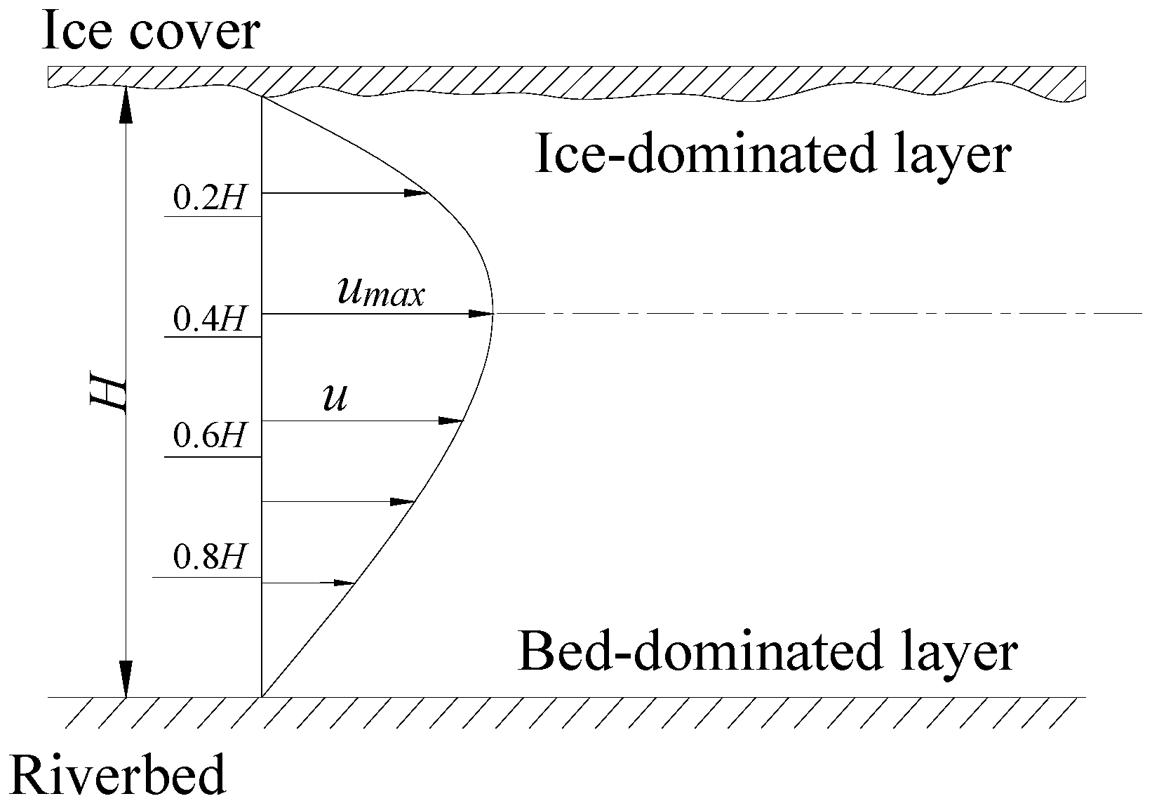
Combining the depth-averaged velocity at a typical survey-point position with the flow depth is used to obtain the entire section-flow discharge by the stream-tube method. The accurate determination of the depth-averaged velocity at the typical survey point is the basis of the aforementioned measurement methods. The accuracy of the depth-averaged velocity has a significant impact on the accuracy of the entire section-flow discharge estimation. Therefore, the commonly used methods for estimating the depth-averaged velocity during the ice-covered period were compared, including the one-, two-, three-, and six-point methods, in addition to the new three-point method proposed by Shan et al. [28] (listed in Table 1). The vertical-velocity distribution under the ice cover and the position of typical measuring points in Table 1 are shown in Figure 2. The coefficient is applied to adjust the point velocity at selected positions to obtain the vertical depth-averaged velocity.
2.2.2. Accuracy of Velocity Estimation of a Single Survey Point
As discussed above, to obtain the flow discharge during ice periods by the stream-tube method, the vertical-flow-velocity distribution or depth-averaged velocity at a certain position must be obtained. Therefore, the accuracy of velocity estimation of a single survey point has an immense impact on the accuracy of flow-discharge measurement.
The relative estimation error ε of the depth-averaged velocity is defined as follows:
where is the depth-averaged velocity estimated using methods shown in Table 1, and U is the actual depth-averaged velocity.
As mentioned previously, the two-power-law expression proposed by Tsai and Ettema [24] has been widely used to describe the vertical-velocity distribution under ice cover [33] to a high level of accuracy. In the absence of measured flow velocities, this study temporarily used Equation (8) instead of the measured or actual depth-averaged velocity to analyze the estimation error. The two-power-law expression is stated as follows:
where is a constant at a given flow discharge, mb and mi are constants related to the flow resistance of the riverbed and ice cover, respectively, H is the total-flow depth, and z is the distance from the riverbed. At z = 0 (riverbed) and z = H (ice-cover bottom), the flow velocity is zero (u = 0).
Disregarding the effect of the boundary layer on flow, q can be obtained by integrating the above equation in the vertical direction:
where β is the Beta function that can be obtained directly from the mathematics manual or the Matlab toolbox.
Based on Equation (9), the depth-averaged velocity under ice cover is expressed as:
3. Results and Discussion
3.1. Accuracy Analysis of Characterization Method of the Depth-Averaged Velocity
The relative estimation errors of the above methods are obtained from Equation (7) and expressions are summarized in Table 2; the calculated values of the vertical depth-averaged velocity of each flow-velocity characterization method are expressed in Equation (8), and the measured values are expressed in Equation (10). The depth-averaged–velocity-estimation accuracy obtained by each method is compared and analyzed based on sixty groups of basic verification data sets.
The verification data include thirty-one sets of flume-test data and twenty-nine sets of natural-channel data. The width-depth ratio (B/H) ranged from 1.22 to 204, and the flow discharge ranged from 0.0114 to 1850 m3/s, involving various cross-sectional forms such as natural channels, rectangular cross-sections, and compound sections. These data and associated parameters are shown in Appendix A Table A1. In Figure 3, Figure 4 and Figure 5, we define rm as the ratio of mb to mi, where rm is represented along the abscissa, and the error percentage is represented along the ordinate; the comparison of the estimation accuracy of each flow-estimation method is discussed below.
- a.
- Comparison of one-point–velocity-estimation methods
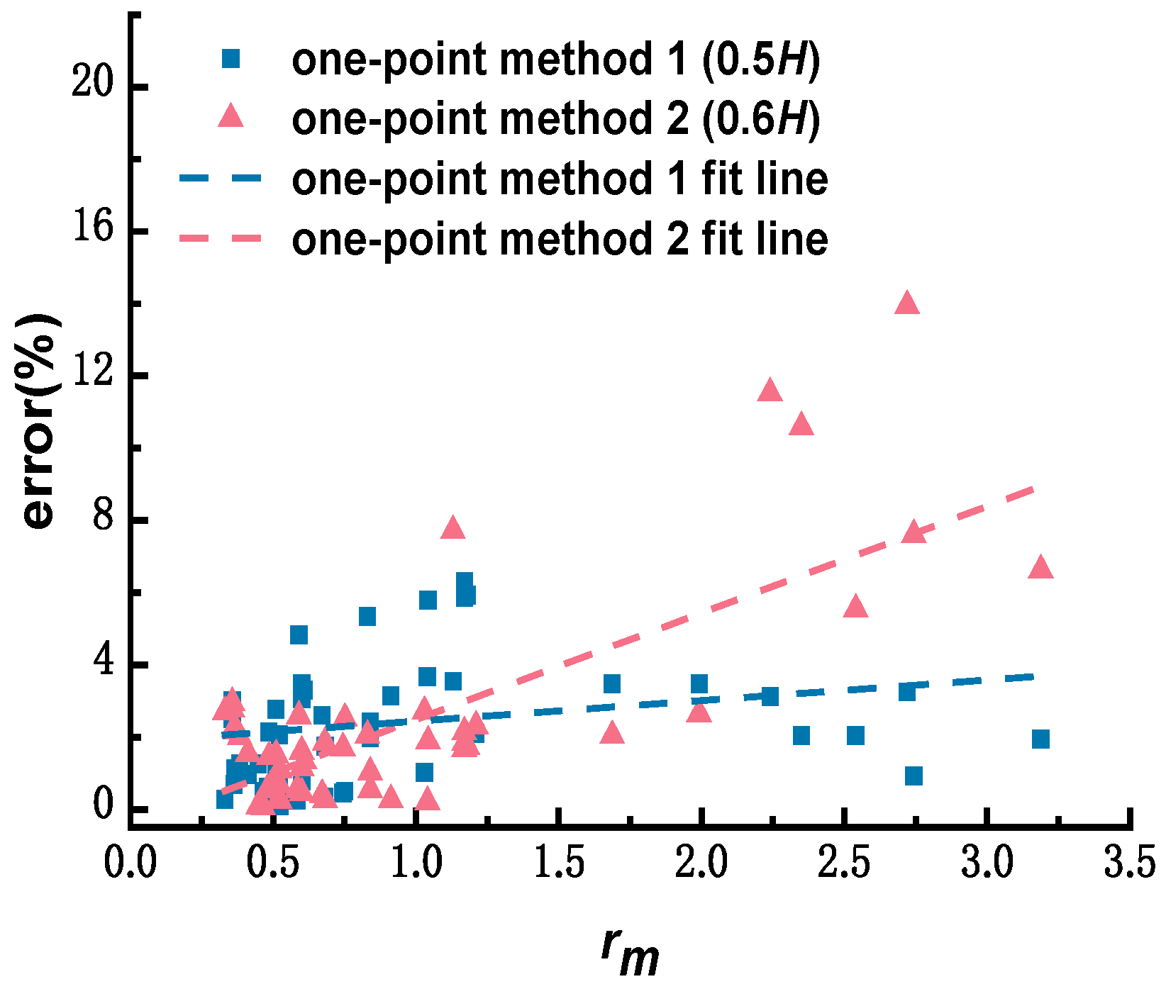
The one-point method at 0.5H and 0.6H were selected, and the commonly used adjustment coefficients of 0.88 and 0.92 [26] were used to compare the errors. The results are shown in Figure 3, where it is observed that the one-point method at 0.5H is relatively stable. The best-fit line representing error margins exhibits a slow upward trend with an increase in rm. Values for rm ranged from 0 to 3.5, and the estimation error of the one-point method at 0.5H was within the range of 6.30%, with an average value of 2.60% and a standard deviation of 1.86. As observed in the figure, the average estimation error of the one-point method at 0.6H is 2.71%, but some values have large deviations; the maximum estimation error is 13.9%, standard deviation is 2.86, and the variation range is large.
- b.
- Comparison of two-point–velocity-estimation methods
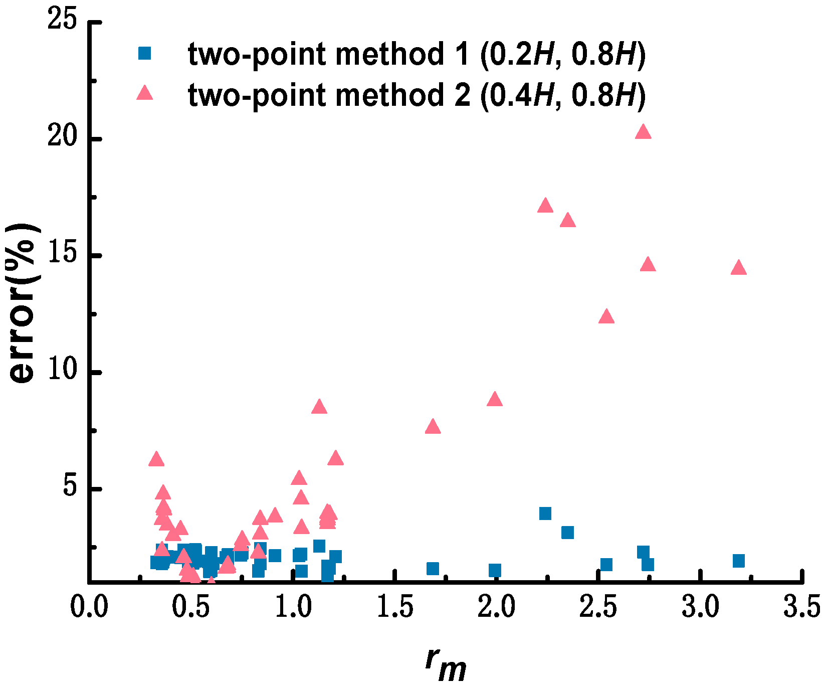
The two-point method at 0.4H and 0.8H and that at 0.2H and 0.8H are mentioned in the ISO standard 9196 [29]. The velocity-estimation accuracy of the two methods is shown in Figure 4, where the estimation accuracy of the two-point method at 0.2H and 0.8H is significantly higher than that at 0.4H and 0.8H, which is consistent with the conclusion presented by Teal [27]. Values for rm ranged from 0 to 3.5, and the estimation error of the two-point method at 0.2H and 0.8H was within the range of 1.29% to 3.95%, with an average value of 1.98%, satisfying the accuracy requirements. Under the same conditions, the average estimation error of the two-point method at 0.4H and 0.8H was 4.85%, and the maximum estimation error was 20.23%.
- c.
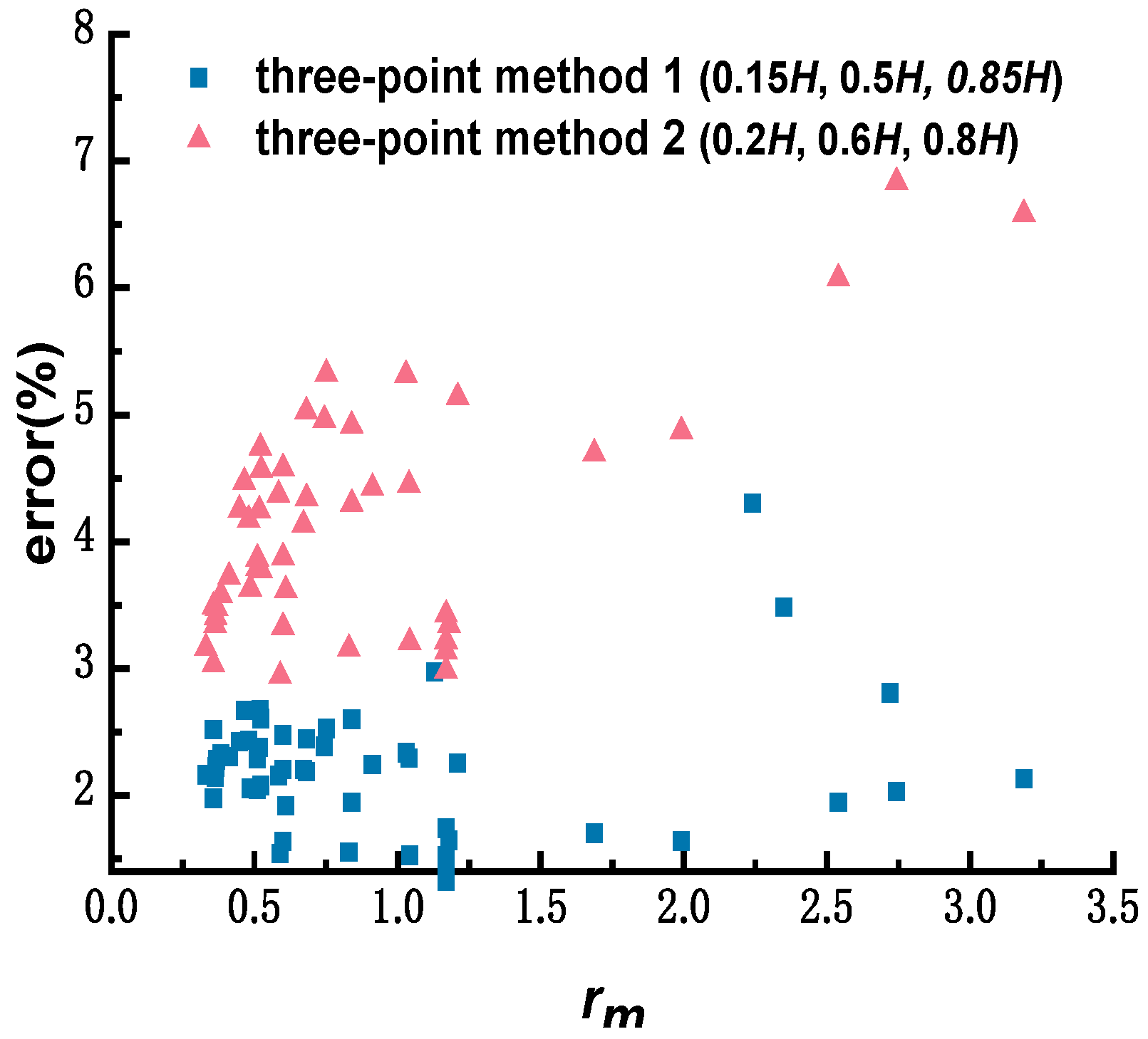
- Comparison of three-point–velocity-estimation methods
The errors in estimating the depth-averaged velocity by the three-point method 1 and the three-point method 2 are given in Figure 5. Here it can be seen the estimated depth-averaged velocity determined by the three-point method 1 was more accurate than that determined by the three-point method 2. Values of rm ranged from 0 to 3.5; the average error estimated by the three-point method 1 at 0.15H, 0.5H, and 0.85H was 2.16%; the maximum estimation error was 4.3%, and the standard deviation was 0.52. The average estimation error using the three-point method 2 at 0.2H, 0.6H, and 0.8H was 4.57%; the maximum estimation error was 9.7%, and the standard deviation was 1.56.
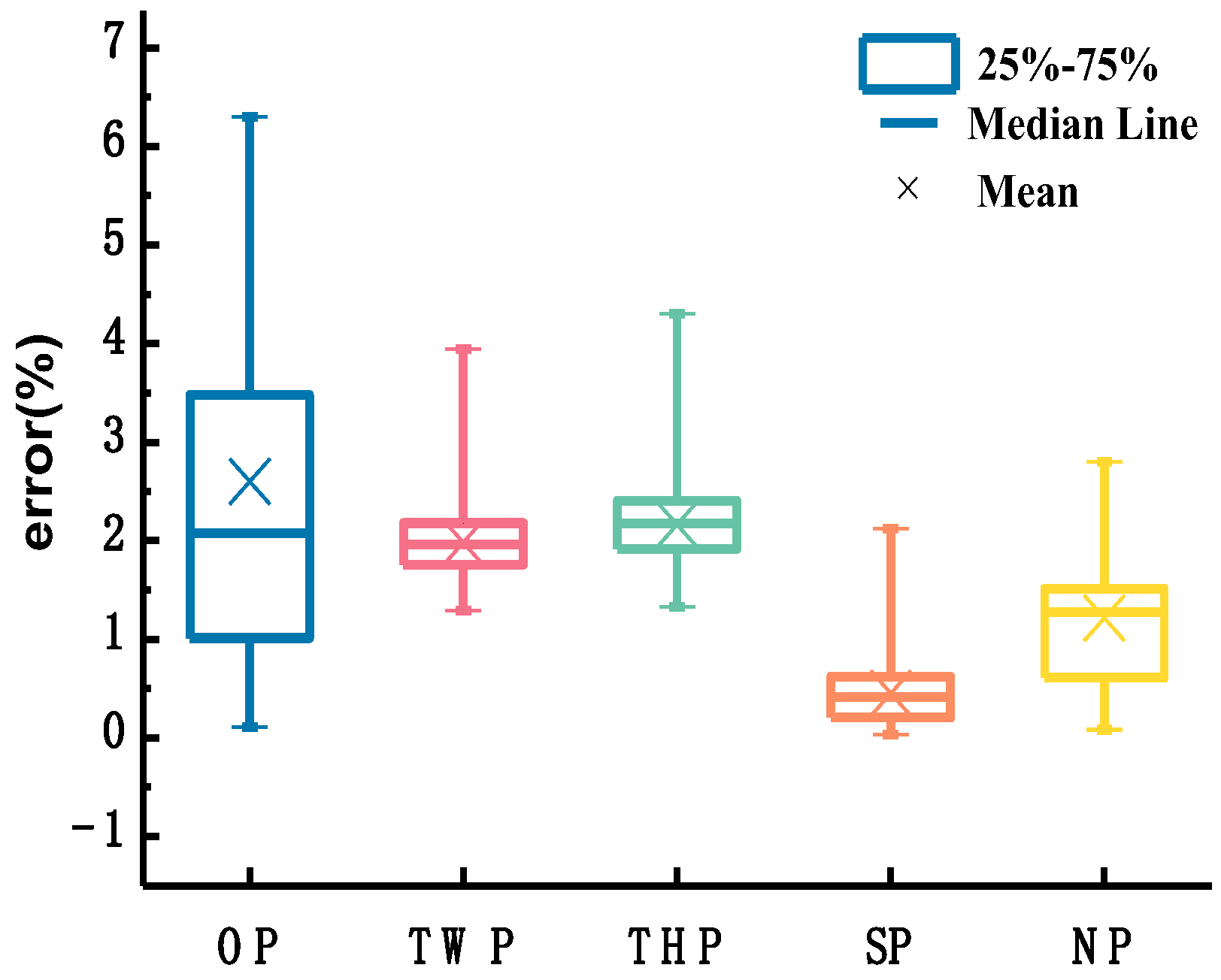
Among the methods given by the ISO specification [29], those with higher estimation accuracies include the one-point method at 0.5H, two-point method at 0.2H and 0.8H, three-point method 1, and six-point method. Taking Shan’s new three-point method into account, the use of quantiles, combined with box diagrams, are used to conduct statistical analysis of the depth-averaged–velocity-estimation errors of the above methods, as shown in Figure 6. This figure illustrates the median, 1/4 quantile, 3/4 quantile, and the maximum and minimum values of the estimation errors for each method. The analysis shows that among the methods listed in the specification, the accuracy of the six-point method is high and the workload of the one-point method is small, but the error fluctuation range is slightly larger. The average error estimated by the six-point method was 0.45%, and the median was 0.41%. The error was mainly distributed between 0.21% and 0.62%; in fact, in many cases it was difficult to arrange six measuring points. The average error and variation range estimated by the three-point method 1 were larger than those estimated by the two-point method at 0.2H and 0.8H. The mean, median, and main error-concentration ranges of the two-point method at 0.2H and 0.8H, and the one-point method at 0.5H, were 1.98%, 1.96%, and 1.76%–2.18%, and 2.6%, 2.08%, and 1.01–3.48%, respectively. When using the one-point method, the depth-averaged velocity is estimated from the velocity at a single point; therefore, the effect of coefficient and single-point-velocity errors may lead to larger estimation error ranges than the other methods. The average estimation error of the three-point method proposed by Shan et al. was 1.22%, and the errors were concentrated in the range of 0.63% to 1.51%. Therefore, the one-point method at 0.5H shows some advantages if only the workload is considered, and the new three-point method proposed by Shan et al. has obvious advantages if the measurement efficiency and accuracy is comprehensively considered.
3.2. Analysis of Position Selection of the Typical Survey-Point
The stream-tube method only requires the vertical-flow-velocity distribution at one typical survey-point position to be measured, provided that the sectional flow-depth distribution is obtained. Thus, the measurement workload of velocity distribution at multiple survey-point positions is reduced. The analysis conducted in Section 3.1 allows the selection of the depth-averaged–velocity-estimation method for estimating the depth-averaged velocity of the typical survey point and allows this to be determined based on the workload and the expected accuracy estimation. However, the analysis shows that the estimation accuracy of flow discharge by the stream-tube method can be influenced by the cross-section characteristic coefficient and the selection of a typical survey-point position.
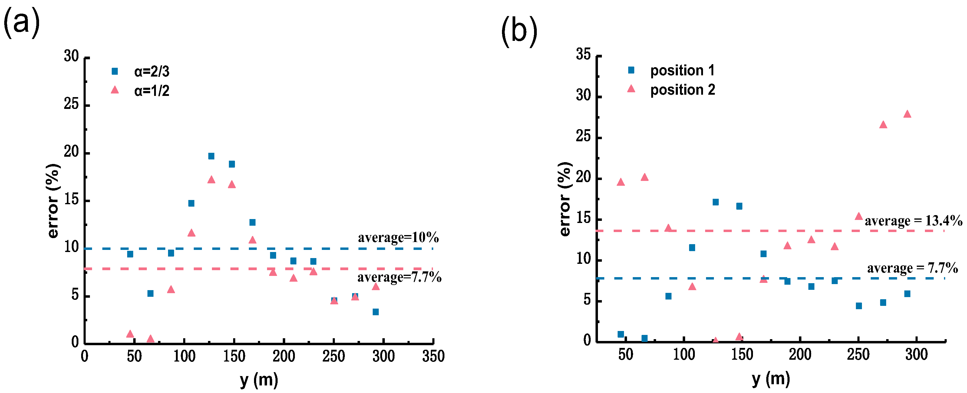
Here, the natural section at the Sanhuhekou of the Yellow River on 21 December 2013, is taken as an example to explain the influence of the cross-section characteristic coefficient and the selection of typical survey-point positions on the flow-discharge estimation accuracy. As shown in Figure 7a, if the survey point is selected at the maximum-flow-depth of the cross-section (thalweg) and the coefficient α is taken as 1/2 and 2/3 in turn, the average estimation error of unit discharge at each measurement point of the cross-section is 7.7% and 10.0%, respectively, calculated by the stream-tube method. As shown in Figure 7b, in natural channels, the coefficient α is taken as 0.5, the survey point is set at any position near the central axis (Figure 7b, position 2), and at the maximum-flow-depth of the cross-section (Figure 7b, position 1) and the average estimation error of unit discharge at each measurement point of the cross-section is 13.4% and 7.7%, respectively. Compared with the position of the survey point, the cross-section characteristic coefficient has less influence on the flow-discharge estimation accuracy using the stream-tube method; therefore, the following analysis focuses on the influence of typical survey-point selection on the estimation accuracy of flow discharge by the stream-tube method.
3.2.1. Relative Unit Discharge Distribution of Common River Cross-Sections
During open-channel-flow discharge measurement, the survey point is typically placed in the mainstream area. According to this principle, the unit discharge at this survey-point position accounts for a large proportion of the total section flow. In addition, systematic errors are inevitably encountered during actual measurement, and the proportion of this error is relatively small when the unit discharge is large. This suggests that selecting a survey point corresponding to a position with larger unit discharge may result in improved estimation accuracy. The relationship between relative-unit discharge and flow depth in river channels with various cross-sectional forms was analyzed as follows.
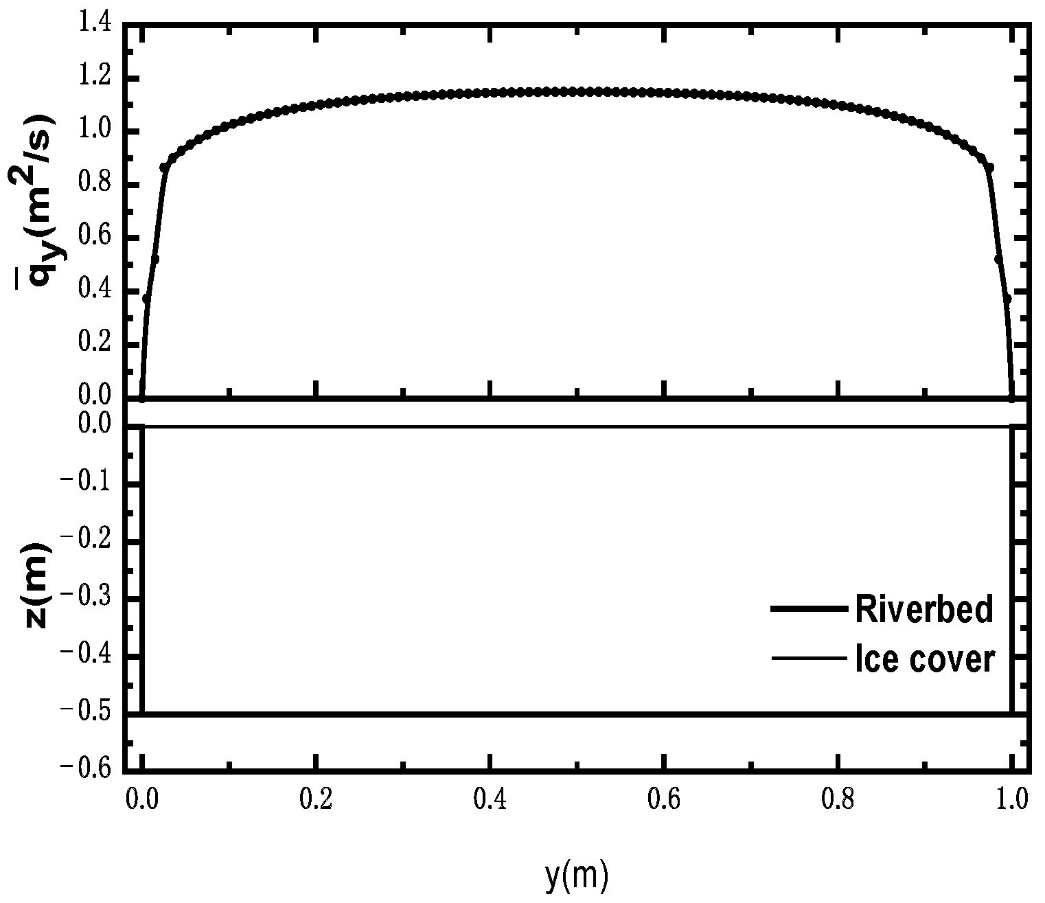
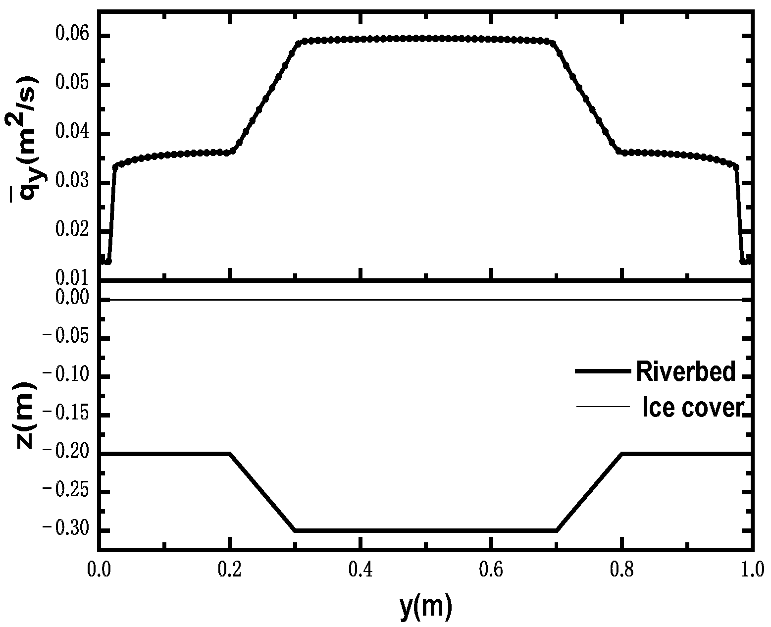
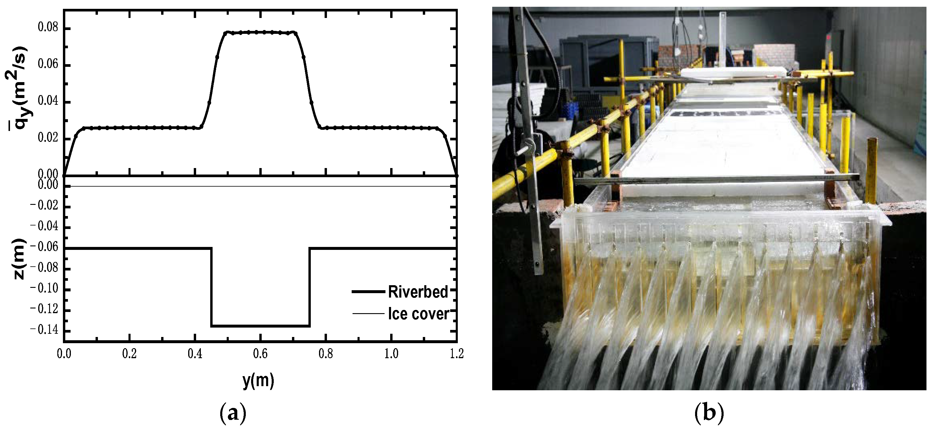
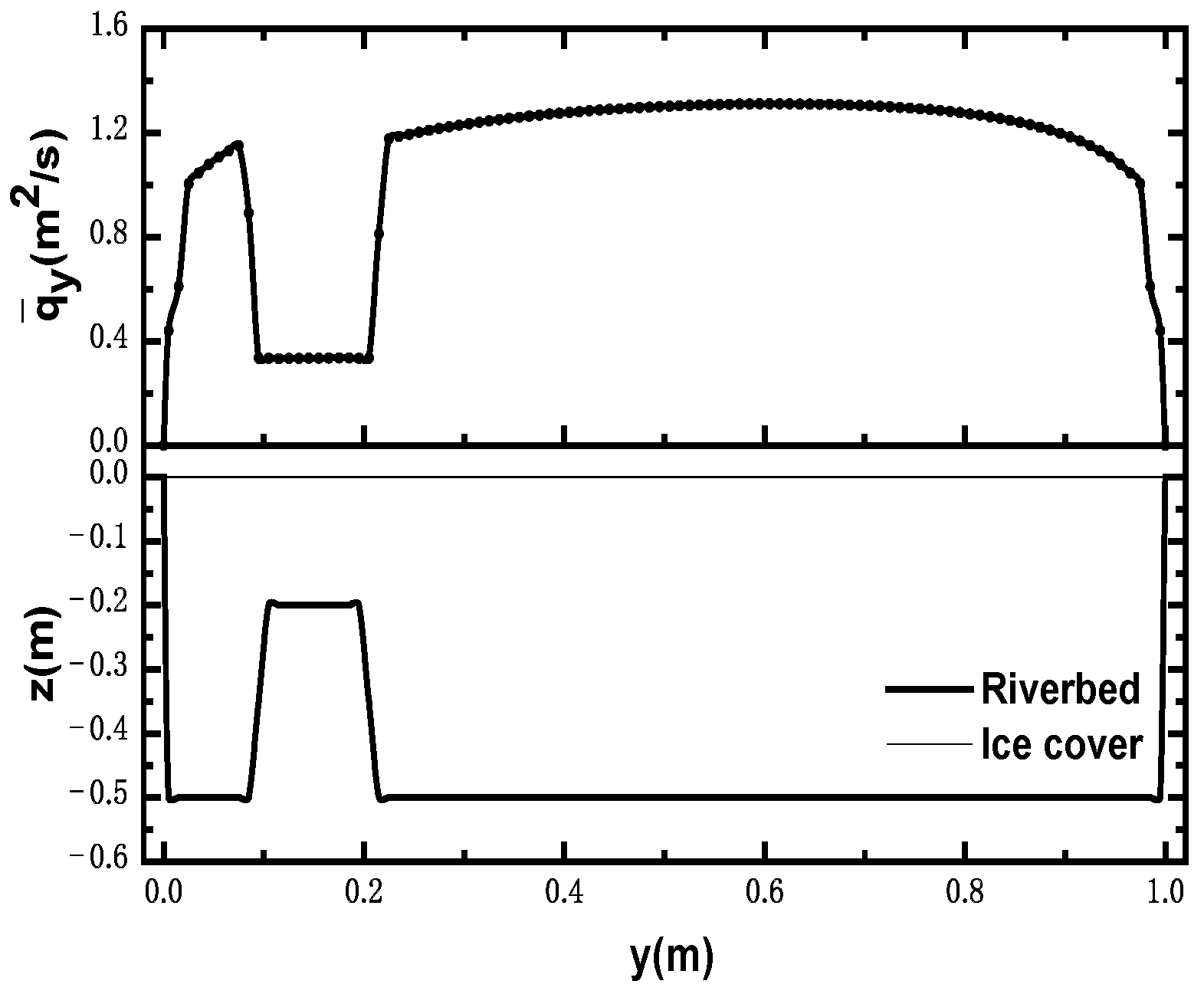
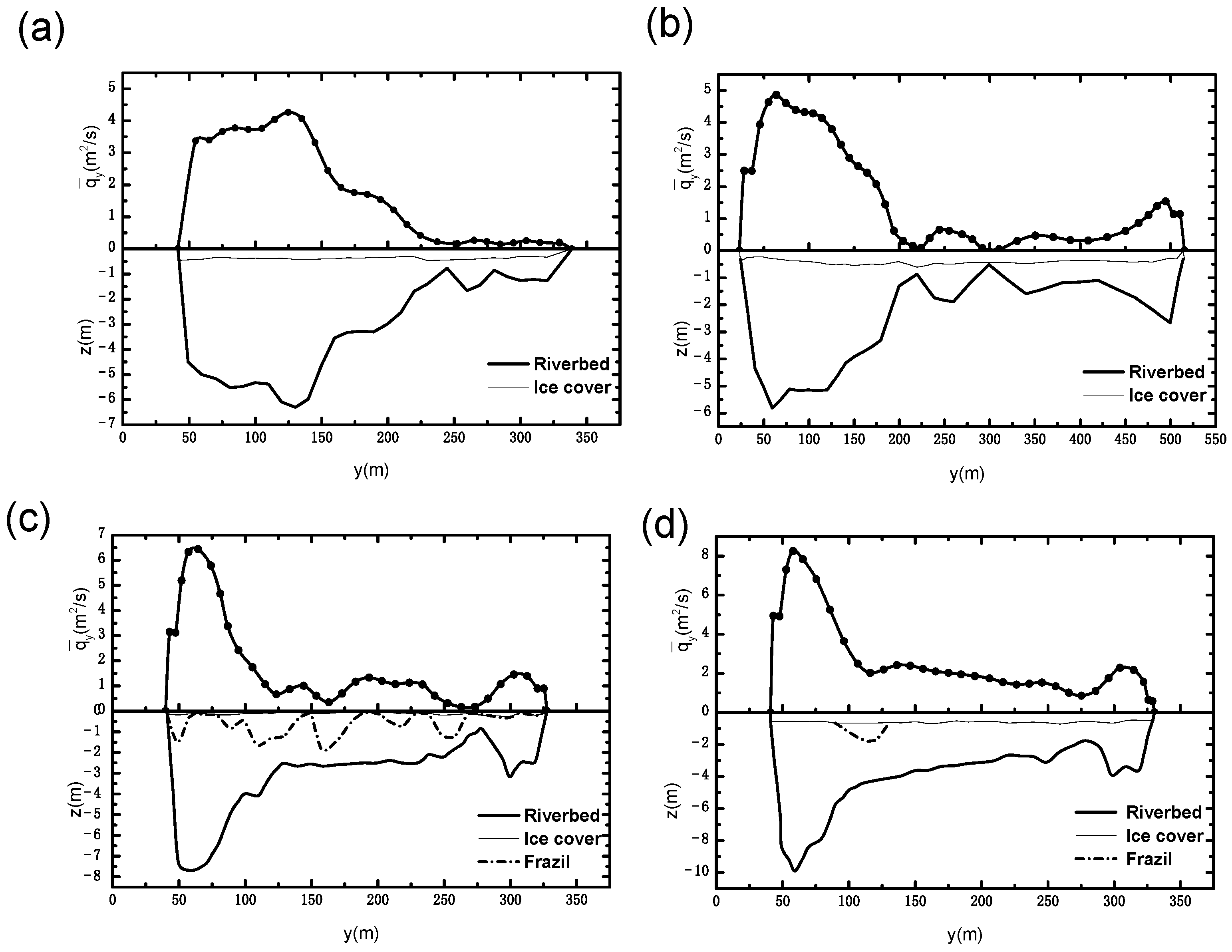
Here, common section forms were chosen, such as rectangular (Figure 8), trapezoidal compound (Figure 9), compound with main channel and floodplain (Figure 10), those containing two thalwegs (Figure 11), and typical natural channels [34,35,36] (Figure 12); then, the relative-unit discharge distribution along these cross-sections was analyzed. In the experimental flume (Figure 10b), the velocity under the ice cover was measured using acoustic Doppler velocimetry (ADV) and particle image velocimetry (PIV). The cross-section characteristic coefficient was taken to be 0.5 and 0.25 for natural and artificial channels, respectively, and the distribution of relative-unit discharge along the cross-section was obtained using Equation (4), as presented in Figure 8, Figure 9, Figure 10, Figure 11 and Figure 12.
Figure 8, Figure 9, Figure 10, Figure 11 and Figure 12 show the section topography, ice-cover distribution, and cross-sectional unit discharge of typical sections. As can be seen, for the rectangular-section channel, the relative-unit discharge distribution along the cross-section is more uniform, and only decreases rapidly near the side wall of the channel. For the compound cross-section channel, the distribution of relative-unit discharge along the cross-section varies greatly, and the distribution along the cross-section increases with an increase in the flow depth. Additionally, the proportion of the relative-unit discharge at the measuring point near the thalweg of the above sections is the largest. When the cross-section has multiple thalwegs (Figure 11), the measuring point near the thalweg in the mainstream area contains a considerable proportion of the relative unit discharge. In general, the distribution of relative unit discharge along the cross-section of the common river cross-sections tends to be consistent with the change in the flow depth, and the figures roughly represent “mirror image” characteristics. The conclusions obtained from the above analysis provide a basis for setting the survey point at the thalweg of the cross-section. To further verify the feasibility of setting the survey point at the thalweg, it is necessary to compare the estimation accuracy of unit discharge at the remaining measuring points of the cross-section.
3.2.2. Influence of the Survey-Point Position on the Cross-Section Discharge Estimation Accuracy
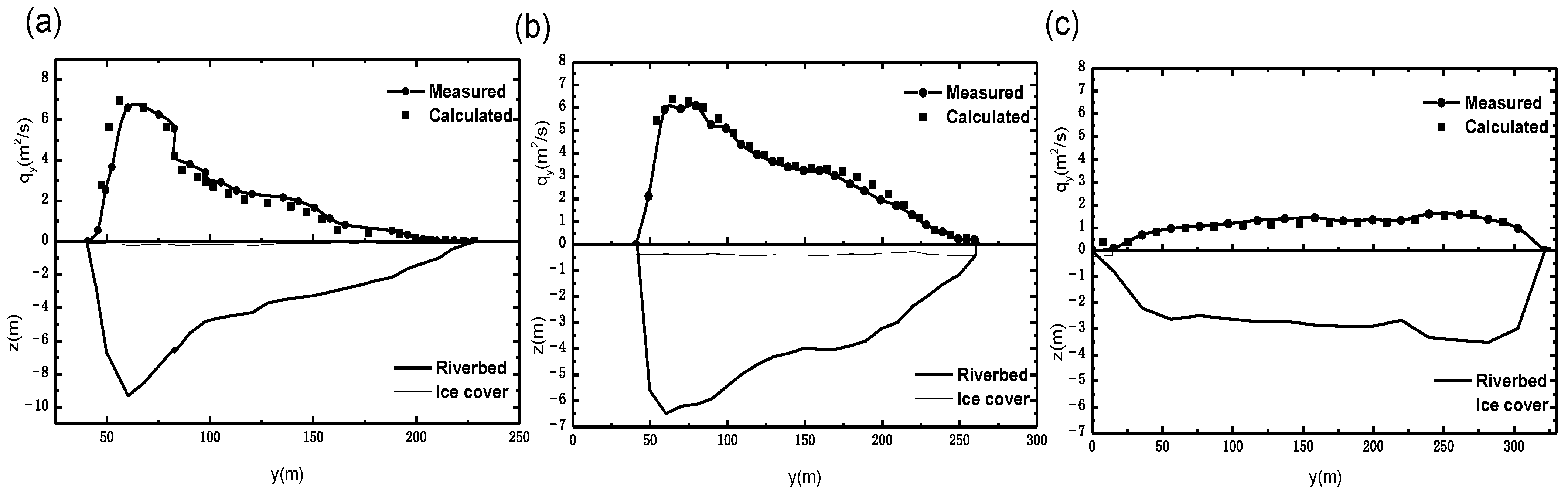
Three natural-river sections of the Yellow River [34] were selected, including the sections of the Baotou and Sanhuhekou Hydrometric Stations. The survey point was set at the thalweg of the section, and the cross-section characteristic coefficient was considered to be 0.5. The estimated and the measured unit discharge at the remaining measuring points of the cross-section was analyzed.
Figure 13 shows a section of the Yellow River during a stable ice-covered period. The three natural-river sections’ topography and ice-cover distribution, in addition to the estimated and measured unit discharge, are depicted in Figure 14a–c. The unit discharge at the remaining measuring points of the cross-section was obtained by setting the survey point at the thalweg in good agreement with measured values. For the three sections shown in Figure 14a–c, the average estimation error of unit discharge obtained by setting the survey point at the thalweg was 13.9%, 12.0%, and 7.7%, and the standard deviation was 7.33, 8.8, and 5.0, respectively. The proportion of the unit discharge deviation in Figure 14a–c shown from left to right within 20% was 93.3%, 86.4%, and 100%, respectively.
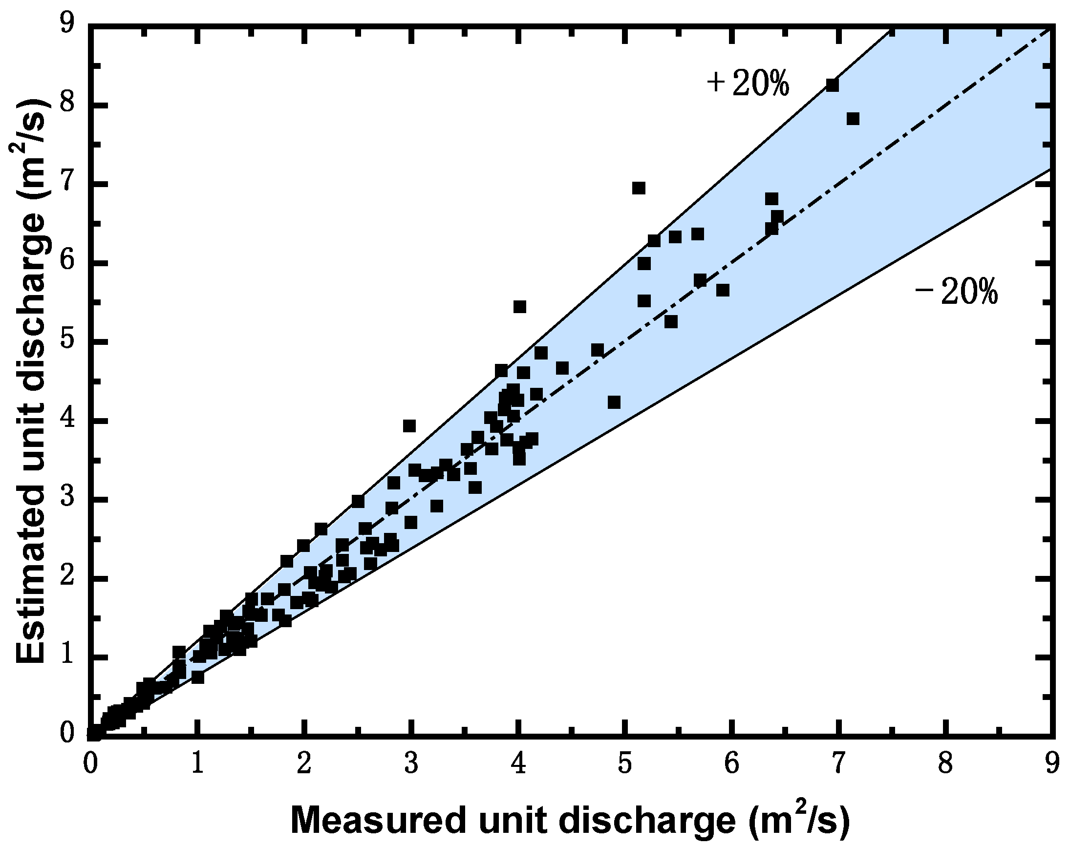
Similarly, the survey point was set at the thalweg of the section, and the cross-section characteristic coefficient was taken to be 0.5 and 0.25 for natural rivers and artificial channels respectively, to obtain the estimated unit discharge along the cross-section of the other sections (Figure 9, Figure 10 and Figure 12). The estimated and measured unit discharge is shown in Figure 15, where the abscissa represents the actual measured unit discharge; the ordinate represents the estimated unit discharge; and the scatter point represents that obtained by setting the survey point at the thalweg. The closer the scatter point to the middle 45° oblique line, the more accurate the estimation result—the shadow area indicates the error range within ±20%. In the given nine sections, the average error of unit discharge is 9.5%, and the error range is within 35.6%; 168 measurement points were selected in the nine sections, among which 90.5% of the estimated unit discharge deviates from the measured value within 20%.
It was preliminarily verified that, when applying the stream-tube method, the cross-section characteristic coefficient was taken to be 0.5 and 0.25 for natural river and artificial channels, respectively, and the survey point was set at the thalweg of the section in the mainstream area. This is not only convenient for actual measurement but can also improve the accuracy of the whole section-flow discharge estimation.
It should be noted that, in applications, simpler and regular cross-sections tend to be selected to obtain relatively high estimation accuracy, and the survey-point position selection method proposed in this study is only applicable to rivers with a single thalweg. For river channels with multiple thalwegs, in most cases, the estimated cross-sectional flow discharge differs when the survey point is taken at different positions of the thalwegs, due to the side wall resistance differences at different positions on the cross-section, resulting in different relative-unit discharge and cross-sectional flow discharges when the survey point is set at two different positions with the same flow depth. In this study, we conducted tests on the river cross-section with two thalwegs. At present, the hydrometric station lacks the measured flow data for multiple thalweg sections in winter, and this conclusion needs to be further verified when these data becomes available.
4. Conclusions
In wider rivers, it is often necessary to drill dozens of holes along the river cross-section, and it is time consuming to measure the velocity in each hole after drilling. Using the stream-tube method, the depth-averaged velocity of a single survey point can be combined with topographic distribution data to determine the overall flow discharge of the entire section, which reduces the measurement workload and improves overall efficiency. However, the measurement accuracy may be influenced by the cross-section characteristic coefficient and the selection of typical survey-point positions. In this study, we compared the depth-averaged velocity-estimation methods, such as the one-, two-, three-, and six-point methods, and their accuracy, by conducting previously researched experiments and laboratory flume model tests, and using natural-river data. Thereafter, we analyzed the relationship between the unit discharge along the cross-section of the common river cross-sections and the cross-sectional flow-depth distribution, in addition to the influence of typical survey-point positions on the estimation accuracy of flow discharge by the stream-tube method. Detailed conclusions can be drawn from this study as follows:
- Contrast analysis of commonly used estimation methods of depth-averaged velocity under ice cover. Based on the selected sixty sets of measured data, the depth-averaged velocity-estimation errors obtained by applying the one-point method at 0.5H, two-point method at 0.2H and 0.8H, three-point method proposed by Shan et al., and six-point method, were calculated as 2.60%, 1.98%, 1.22%, and 0.45%, respectively, and the corresponding standard deviations were 1.86, 0.44, 0.62, and 0.35, respectively. The one-point method at 0.5H is appropriate for estimating the depth-averaged velocity of a single line, depending on the workload. If the workload increases, the two-point method at 0.2H and 0.8H may be chosen. If the measurement conditions can meet the arrangement of three measuring points, depending on the measurement efficiency and accuracy, the new three-point method proposed by Shan et al. is recommended. The reasonable and accurate selection of the estimation methods of depth-averaged velocity under ice cover further reduces the workload in the application of the stream-tube method.
- By analyzing the parameter sensitivity of the flow-discharge measurement accuracy to the cross-section characteristic coefficient α and the typical survey-point position, the latter was found to have less influence on the flow-discharge measurement accuracy of the stream-tube method compared to the typical survey-point position. The cross-section characteristic coefficient was taken to be 0.5 and 0.25 for natural rivers and artificial channels, respectively. By analyzing the relationship between the relative unit discharge distributions of common river cross-sections and the cross-sectional flow-depth distributions, the survey point should be set at the thalweg of the section in the mainstream area. Using the proposed method at this suggested survey-point position, the percentage of measurement points with an estimated error of unit discharge less than 20% within the selected cross-section, including the laboratory flume model tests and natural-river data, reached 90.5% of all the measuring points.
For practical applications, the survey point is arranged at the thalweg of the cross-section, and the estimation method of the depth-averaged velocity of the typical survey point is determined according to the expected measurement accuracy and workload. Combined with the section topography, the entire section-flow discharge can be obtained, which improves the acquisition efficiency of flow velocity data under ice cover and the accuracy of the flow-discharge estimation for the entire section.
Author Contributions
Conceptualization, J.L. and X.G.; methodology, J.L. and J.P.; formal analysis, X.G., H.F. and Y.W.; writing—original draft preparation, J.L.; writing—review and editing, J.L., X.G. and J.P.; supervision, Y.W. and Z.M.; funding acquisition, X.G. and H.F. All authors have read and agreed to the published version of the manuscript.
Funding
This research was funded by the National Key Research & Development Plan of China (2022YFC3202500), the National Natural Science Foundation of China (U2243221, 52009144), and IWHR Research & Development Support Program (HY110145B0012021, HY0145B032021).
Data Availability Statement
Data are contained within the article.
Acknowledgments
We thank everyone who helped us during the completion of the thesis. We also thank the reviewers for their useful comments and suggestions.
Conflicts of Interest
The authors declare no conflict of interest.
Appendix A

Table A1.
Hydraulic parameters and flow characteristics for error estimation in ice-covered channels.
Table A1.
Hydraulic parameters and flow characteristics for error estimation in ice-covered channels.
| Data Source | Test | Discharge (m3/s) | Width Depth Ratio (B/H) | Resistance Parameter | ||
|---|---|---|---|---|---|---|
| mb | mi | rm | ||||
| Tatinclaux and Gogus [37] | Athabasca R., AL | 1850.00 | 85.00 | 5.73 | 2.44 | 2.35 |
| Athabasca R., AL | 1230.00 | 106.00 | 5.47 | 2.44 | 2.24 | |
| Athabasca R., AL | 850.00 | 121.00 | 5.04 | 1.85 | 2.72 | |
| Engmann [38] | 101 | 7.10 × 10⁻³ | 1.22 | 3.10 | 6.46 | 0.48 |
| 102 | 15.60 × 10⁻³ | 1.22 | 4.12 | 8.08 | 0.51 | |
| 103 | 12.70 × 10⁻³ | 1.22 | 4.60 | 7.54 | 0.61 | |
| 104 | 11.40 × 10⁻³ | 1.22 | 4.60 | 7.54 | 0.61 | |
| Parthasarathy and Muste [39] | R1 | 50.10 × 10⁻³ | 4.20 | 4.59 | 7.65 | 0.60 |
| R2 | 50.10 × 10⁻³ | 3.70 | 4.90 | 5.83 | 0.84 | |
| R3 | 50.10 × 10⁻³ | 3.10 | 4.70 | 4.56 | 1.03 | |
| Smith and Ettema [40] | S2 | 78.70 × 10⁻³ | 4.90 | 7.02 | 8.46 | 0.83 |
| M2 | 75.50 × 10⁻³ | 4.70 | 6.63 | 6.38 | 1.04 | |
| R2 | 75.40 × 10⁻³ | 4.40 | 5.73 | 4.74 | 1.21 | |
| S4 | 76.30 × 10⁻³ | 5.00 | 4.51 | 7.52 | 0.60 | |
| M4 | 75.30 × 10⁻³ | 4.80 | 4.79 | 5.70 | 0.84 | |
| R4 | 74.50 × 10⁻³ | 4.40 | 4.70 | 4.56 | 1.03 | |
| Wei and Huang [41] | Case 1 | 50.10 × 10⁻³ | 2.10 | 9.68 | 8.27 | 1.17 |
| Case 2 | 50.10 × 10⁻³ | 2.10 | 9.68 | 8.27 | 1.17 | |
| Case 3 | 50.10 × 10⁻³ | 2.10 | 9.68 | 8.27 | 1.17 | |
| Case 4 | 69.90 × 10⁻³ | 2.30 | 9.58 | 8.19 | 1.17 | |
| Case 5 | 60.00 × 10⁻³ | 2.50 | 9.48 | 8.10 | 1.17 | |
| Case 6 | 40.10 × 10⁻³ | 3.00 | 9.26 | 7.91 | 1.17 | |
| Case 7 | 30.30 × 10⁻³ | 3.50 | 9.26 | 7.91 | 1.17 | |
| Case 8 | 50.70 × 10⁻³ | 2.30 | 9.58 | 8.12 | 1.18 | |
| Case 10 | 50.00 × 10⁻³ | 2.60 | 8.00 | 3.15 | 2.54 | |
| Case 11 | 60.20 × 10⁻³ | 2.40 | 8.00 | 3.15 | 2.54 | |
| Case 12 | 50.20 × 10⁻³ | 2.50 | 8.00 | 3.15 | 2.54 | |
| Case 13 | 50.20 × 10⁻³ | 2.50 | 8.00 | 3.15 | 2.54 | |
| Case 15 | 50.70 × 10⁻³ | 2.10 | 3.45 | 3.05 | 1.13 | |
| Case 16 | 41.20 × 10⁻³ | 2.30 | 3.45 | 3.05 | 1.13 | |
| Attar and Li [33] | Salmon R., NB | 12.00 | 3.70 | 3.36 | 4.93 | 0.68 |
| S.W. Miramichi R., NB | 51.00 | 3.10 | 3.59 | 7.39 | 0.49 | |
| R. John, NS | 2.00 | 4.90 | 8.52 | 8.17 | 1.04 | |
| Kaministiquia R., ON | 43.00 | 4.70 | 4.10 | 6.01 | 0.68 | |
| Saugeen R., ON | 29.00 | 4.40 | 2.89 | 5.55 | 0.52 | |
| Nith R., ON | 1.50 | 5.00 | 4.54 | 6.76 | 0.67 | |
| Burnt R., ON | 10.00 | 4.80 | 3.20 | 5.48 | 0.58 | |
| Eels Cr.,ON | 1.94 | 4.40 | 3.78 | 5.08 | 0.74 | |
| Moira R., ON | 2.22 | 25.97 | 2.95 | 7.70 | 0.38 | |
| Salmon R., ON | 4.73 | 23.53 | 2.45 | 5.47 | 0.45 | |
| Upper Humber R., NF | 64.00 | 69.44 | 2.79 | 7.58 | 0.37 | |
| Terra Nova R., NF | 25.00 | 33.50 | 2.61 | 7.19 | 0.36 | |
| Groundhog R., ON | 86.00 | 51.03 | 3.50 | 4.66 | 0.75 | |
| Oldman R., AB | 2.33 | 136.00 | 2.94 | 7.14 | 0.41 | |
| Red Deer R., AB | 18.00 | 97.96 | 2.79 | 7.64 | 0.37 | |
| N.SaskatchewanR.,SK | 116.00 | 204.00 | 3.75 | 10.51 | 0.36 | |
| Ou’Appelle R., SA | 1.14 | 37.50 | 5.70 | 6.25 | 0.91 | |
| Beaver R., AB | 2.69 | 41.82 | 2.36 | 7.14 | 0.33 | |
| Pembina R., AB | 12.00 | 105.71 | 3.23 | 6.25 | 0.52 | |
| Halfway R., BC | 7.40 | 72.22 | 2.77 | 5.96 | 0.46 | |
| Litle Smoky R., AB | 11.50 | 97.50 | 3.22 | 9.02 | 0.36 | |
| Peace R., NWT | 1111.00 | 116.70 | 5.44 | 9.22 | 0.59 | |
| Yellowknife R., NWT | 24.00 | 24.00 | 3.55 | 5.92 | 0.60 | |
| Fraser R., BC | 32.00 | 73.08 | 3.25 | 6.37 | 0.51 | |
| Takhini R. YT | 14.00 | 32.86 | 3.12 | 5.96 | 0.52 | |
| Yukon R., YT | 246.00 | 58.00 | 3.69 | 7.06 | 0.52 | |
| Lu [34] | 2.1–2.3 floodplain | 0.05–0.09 | 4.50–9.00 | 7.28 | 2.66 | 2.74 |
| 3.1–3.3 floodplain | 0.05–0.09 | 4.50–9.00 | 9.08 | 2.85 | 3.19 | |
| 2.1–2.3 main channel | 0.05–0.09 | 3.00–5.00 | 7.62 | 4.52 | 1.69 | |
| 3.1–3.3 main channel | 0.05–0.09 | 3.00–5.00 | 8.25 | 4.14 | 1.99 | |
References
- Rokaya, P.; Budhathoki, S.; Lindenschmidt, K.E. Trends in the timing and magnitude of ice-jam floods in Canada. Sci. Rep. 2018, 8, 5834. [Google Scholar] [CrossRef] [PubMed] [Green Version]
- Ettema, R. Review of alluvial-channel responses to river ice. J. Cold Reg. Eng. 2002, 16, 191–217. [Google Scholar] [CrossRef]
- Lees, K.; Clark, S.P.; Malenchak, J.; Chanel, P. Characterizing ice cover formation during freeze-up on the regulated Upper Nelson River, Manitoba. J. Cold Reg. Eng. 2021, 35, 04021009. [Google Scholar] [CrossRef]
- Healy, D.; Hicks, F.E. Index velocity methods for winter discharge measurement. Can. J. Civil Eng. 2004, 31, 407–419. [Google Scholar] [CrossRef]
- Yang, K.L. Lateral distribution of depth-averaged velocities in ice-covered channels. J. Hydraul. Eng. 2015, 46, 291–297. (In Chinese) [Google Scholar]
- Peters, M.; Dow, K.; Clark, S.P.; Malenchak, J.; Danielson, D. Experimental investigation of the flow characteristics beneath partial ice covers. Cold Reg. Sci. Technol. 2017, 142, 69–78. [Google Scholar] [CrossRef]
- Kimiaghalam, N.; Clark, S.P.; Dow, K. Flow characteristics of a partially-covered trapezoidal channel. Cold Reg. Sci. Technol. 2018, 155, 280–288. [Google Scholar] [CrossRef]
- Wang, J.; Sui, J.Y.; Karney, B.W. Incipient motion of non-cohesive sediment under ice cover—An experimental study. J. Hydrodyn. 2008, 20, 117–124. [Google Scholar] [CrossRef]
- Wang, J.; He, L.; Chen, P.P.; Sui, J.Y. Numerical simulation of mechanical breakup of river ice-cover. J. Hydrodyn. 2013, 25, 415–421. [Google Scholar] [CrossRef]
- Alfredsen, K. An assessment of ice effects on indices for hydrological alteration in flow regimes. Water 2017, 9, 914. [Google Scholar] [CrossRef] [Green Version]
- Beltaos, S.; Burrell, B.C. Effects of river-ice breakup on sediment transport and implications to stream environments: A review. Water 2021, 13, 2541. [Google Scholar] [CrossRef]
- Hu, H.T.; Wang, J.; Cheng, T.J.; Hou, Z.X.; Sui, J.Y. Channel bed deformation and ice jam evolution around bridge piers. Water 2022, 14, 1766. [Google Scholar] [CrossRef]
- Fulton, J.W.; Henneberg, M.F.; Mills, T.J.; Kohn, M.S.; Epstein, B.; Hittle, E.A.; Damschen, W.C.; Laveau, C.D.; Lambrecht, J.M.; Farmer, W.H. Computing under-ice discharge: A proof-of-concept using hydro acoustics and the Probability Concept. J. Hydrol. 2018, 562, 733–748. [Google Scholar] [CrossRef]
- Lama, G.F.C.; Errico, A.; Pasquino, V.; Mirzaei, S.; Preti, F.; Chirico, G.B. Velocity uncertainty quantification based on riparian vegetation indices in open channels colonized by phragmites australis. J. Ecohydraulics 2022, 7, 71–76. [Google Scholar] [CrossRef]
- Lama, G.F.C.; Sadeghifar, T.; Azad, M.T.; Sihag, P.; Kisi, O. On the indirect estimation of wind wave heights over the southern coasts of caspian sea: A comparative analysis. Water 2022, 4, 843. [Google Scholar] [CrossRef]
- Khan, M.A.; Sharma, N.; Lama, G.F.C.; Hasan, M.; Garg, R.; Busico, G.; Alharbi, R.S. Three-Dimensional Hole Size (3DHS) approach for water flow turbulence analysis over emerging sand bars: Flume-scale experiments. Water 2022, 14, 1889. [Google Scholar] [CrossRef]
- Walker, J.F. Accuracy of selected techniques for estimating ice-affected streamflow. J Hydraul. Eng. 1991, 117, 697–712. [Google Scholar] [CrossRef]
- Shen, H.T.; Ackermann, N.L. Wintertime flow distribution in river channels. J. Hydraul. Div. 1980, 106, 805–817. [Google Scholar] [CrossRef]
- Pan, J.J.; Guo, X.L.; Wang, T.; Fu, H.; Li, J.Z.; Guo, Y.Y. A novel technique for flow discharge and depth-averaged streamwise velocity in ice periods based on stream tube methods. J. Hydraul. Eng. 2020, 51, 1536–1543. (In Chinese) [Google Scholar]
- Lau, Y.L. Velocity distributions under floating covers. Can. J. Civil Eng. 1982, 9, 76–83. [Google Scholar] [CrossRef]
- Mao, Z.Y.; Luo, S.; Zhao, S.W.; Xiang, P.; Yue, G.X. Study on the velocity distributions for ice-covered flow. Adv. Water Sci. 2006, 17, 209–215. (In Chinese) [Google Scholar]
- Shiono, K.; Knight, D.W. Turbulent open-channel flows with variable depth across the channel. J. Fluid Mech. 1991, 222, 617–646. [Google Scholar] [CrossRef]
- Odgaard, A.J. River-meander model. I: Development. J. Hydraul. Eng. 1989, 115, 1433–1450. [Google Scholar] [CrossRef]
- Tsai, W.F.; Ettema, R. Ice cover influence on transverse bed slopes in a curved alluvial channel. J. Hydraul. Res. 1994, 32, 561–581. [Google Scholar] [CrossRef]
- Walker, J.; Wang, D.F. Measurement of flow under ice covers in North America. J. Hydraul. Eng. 1997, 123, 1037–1040. [Google Scholar] [CrossRef]
- Walker, J.F. Methods for measuring discharge under ice cover. J. Hydraul. Eng. 1994, 120, 1327–1336. [Google Scholar] [CrossRef]
- Teal, M.; Ettema, R.J.; Walker, J.F. Estimation of mean flow velocity in ice-covered channels. J. Hydraul. Eng. 1994, 120, 1385–1400. [Google Scholar] [CrossRef]
- Shan, H.; Kerenyi, K.; Patel, N.; Guo, J. Laboratory test of second log-wake law for effects of ice cover and wind shear stress on river velocity distributions. J. Cold Reg. Eng. 2022, 36, 04022001. [Google Scholar] [CrossRef]
- ISO 9196; Liquid Flow Measurement in Open Channels Flow Measurements under Ice Conditions. International Organisation for Standardisation: Geneva, Switzerland, 1992.
- Einstein, H.A. Formulas for the transportation of bed-load. Trans. ASCE 1942, 107, 561–597. [Google Scholar] [CrossRef]
- Fu, H.; Liu, Z.P.; Guo, X.L.; Cui, H.T. Double-frequency ground penetrating radar for measurement of ice thickness and water depth in rivers and canals: Development, verification and application. Cold Reg. Sci. Technol. 2018, 154, 85–94. [Google Scholar] [CrossRef]
- Su, L.P. Study on the calculation method of vertical average velocity of cross section by three point method. Yangtze River 1982, 1, 76–80. (In Chinese) [Google Scholar]
- Attar, S.; Li, S.S. Data-fitted velocity profiles for ice-covered rivers. Can. J. Civil Eng. 2012, 39, 334–338. [Google Scholar] [CrossRef]
- Lu, J.Z. Theoretical and Experimental Study on the Mechanism of Ice River Coupling in Compound Open Channel. Master’s Thesis, China Institute of Water Resources and Hydropower Research, Beijing, China, 2020. (In Chinese). [Google Scholar]
- Wang, F.F.; Huai, W.X.; Liu, M.Y.; Fu, X.C. Modeling depth-averaged streamwise velocity in straight trapezoidal compound channels with ice cover. J. Hydrol. 2020, 585, 124336. [Google Scholar] [CrossRef]
- Wang, C.Q.; Wang, P.W.; Fan, M.H.; Chen, D.L.; Liu, J.F. Study on Temperature Prediction and Ice Condition Observation Technology in Inner Mongolia Reach of the Yellow River; China Water & Power Press: Beijing, China, 2017. [Google Scholar]
- Tatinclaux, J.C.; Gogus, M. Asymmetric plane flow with application to ice jams. J. Hydraul. Eng. 1983, 109, 1540–1554. [Google Scholar] [CrossRef]
- Engmann, E.O. Turbulent diffusion in channels with a surface cover. J. Hydraul. Res. 1977, 15, 327–335. [Google Scholar] [CrossRef]
- Parthasarathy, R.; Muste, M.N. Velocity measurements in asymmetric turbulent channel flows. J. Hydraul. Eng. 1994, 120, 1000–1020. [Google Scholar] [CrossRef]
- Smith, B.; Ettema, R.T. Flow resistance in ice-covered alluvial channels. J. Hydraul. Eng. 1997, 123, 592–599. [Google Scholar] [CrossRef]
- Wei, L.Y.; Huang, J.Z. Composite manning roughness coefficient of ice-covered flow. Engrg J. WHU 2002, 4, 1–8. (In Chinese) [Google Scholar]
- Chen, G.; Gu, S.X.; Li, B.; Zhou, M.; Huai, W.X. Physically based coefficient for streamflow estimation in ice-covered channels. J. Hydrol. 2018, 563, 470–479. [Google Scholar] [CrossRef]
Figure 1.
Flow profile is divided into bed- and ice-dominated layers: (a) entire cross-section; (b) partial cross-section.
Figure 1.
Flow profile is divided into bed- and ice-dominated layers: (a) entire cross-section; (b) partial cross-section.

Figure 2.
Vertical-flow structure under ice cover.

Figure 3.
Comparison of velocity-estimation error related to two one-point methods.

Figure 4.
Comparison of velocity-estimation error related to two two-point methods.

Figure 5.
Comparison of velocity-estimation error related to two three-point methods.

Figure 6.
Comparison of velocity-estimation errors obtained from various depth-averaged velocity characterization methods (the one-point method at 0.5H, two-point method at 0.2H and 0.8H, three-point method 1, six-point method, and the new method proposed by Shan et al. are indicated along the abscissa).

Figure 7.
Parameter sensitivity analysis: (a) the effect of the cross-section characteristic coefficient α on the estimation error of unit discharge at each measurement point of the cross-section with a constant survey-point position; (b) the effect of the survey-point position on the estimation error of unit discharge at each measurement point of the cross-section with a cross-section characteristic coefficient α of 0.5.

Figure 8.
Section topography showing ice cover and riverbed distribution, and cross-sectional relative-unit discharge in a rectangular section.
Figure 8.
Section topography showing ice cover and riverbed distribution, and cross-sectional relative-unit discharge in a rectangular section.

Figure 9.
Section topography showing ice cover and riverbed distribution, and cross-sectional relative-unit discharge in a trapezoidal compound section.
Figure 9.
Section topography showing ice cover and riverbed distribution, and cross-sectional relative-unit discharge in a trapezoidal compound section.

Figure 10.
Experimental flume section with main channel and floodplain: (a) section topography showing ice cover, riverbed distribution, and cross-sectional relative-unit discharge; (b) photo of experimental flume.
Figure 10.
Experimental flume section with main channel and floodplain: (a) section topography showing ice cover, riverbed distribution, and cross-sectional relative-unit discharge; (b) photo of experimental flume.

Figure 11.
Section topography showing ice cover and riverbed distribution and cross-sectional relative-unit discharge in a channel section with two thalwegs.
Figure 11.
Section topography showing ice cover and riverbed distribution and cross-sectional relative-unit discharge in a channel section with two thalwegs.

Figure 12.
Section topography showing ice cover and riverbed distribution, and cross-sectional relative-unit discharge: (a) Baotou section on 26 January 2014; (b) Dabusutai section on 21 February 2014; (c) Baotou section on 14 December 2014; (d) Baotou section on 23 January 2015.
Figure 12.
Section topography showing ice cover and riverbed distribution, and cross-sectional relative-unit discharge: (a) Baotou section on 26 January 2014; (b) Dabusutai section on 21 February 2014; (c) Baotou section on 14 December 2014; (d) Baotou section on 23 January 2015.

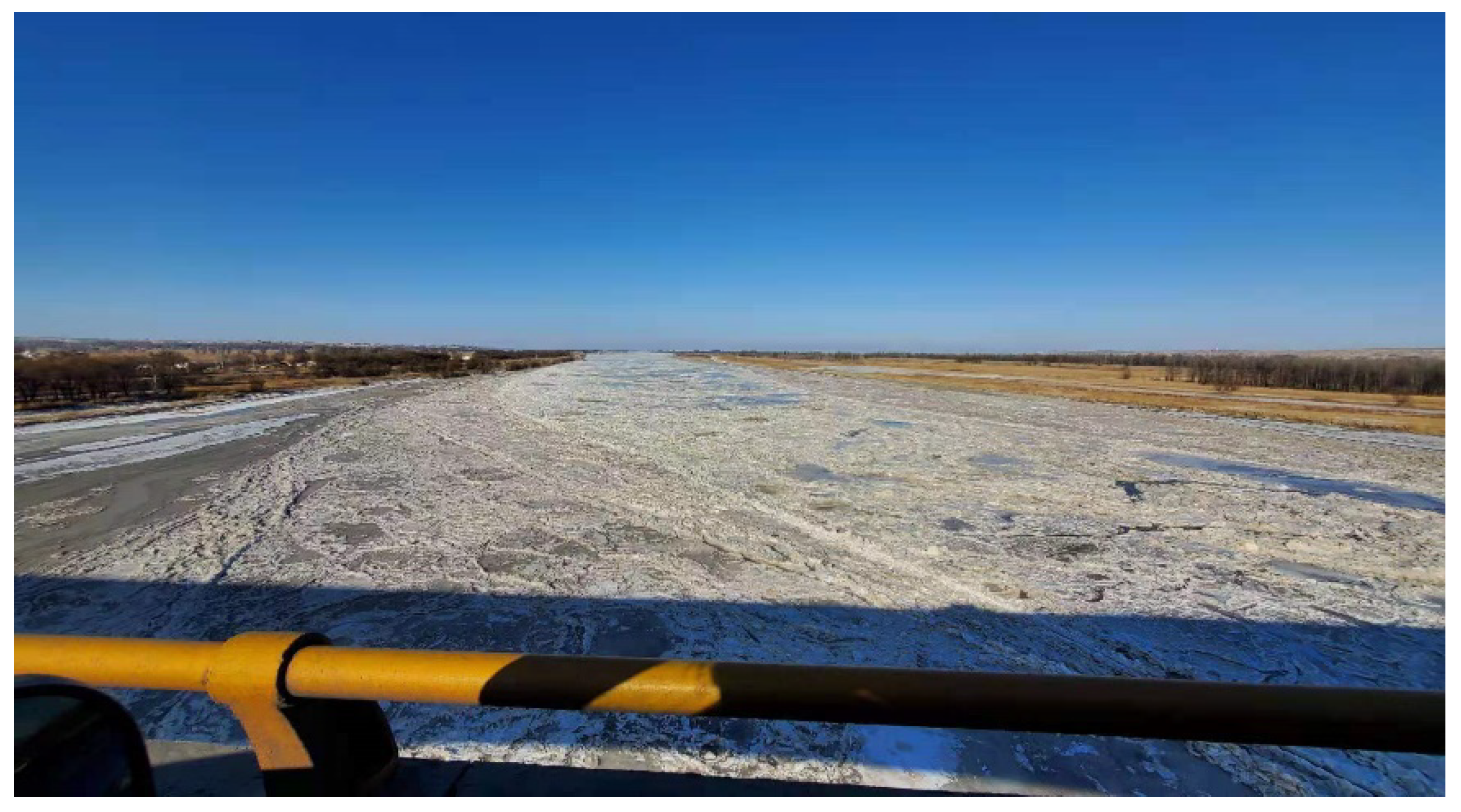
Figure 13.
A section of the Yellow River during a stable ice-covered period.

Figure 14.
Section topography showing ice-cover and riverbed distribution, and the comparison of estimated and measured unit discharge: (a) Baotou section on 10 March 2015; (b) Baotou section on 18 February 2015; (c) Sanhuhekou section on 21 December 2013.
Figure 14.
Section topography showing ice-cover and riverbed distribution, and the comparison of estimated and measured unit discharge: (a) Baotou section on 10 March 2015; (b) Baotou section on 18 February 2015; (c) Sanhuhekou section on 21 December 2013.

Figure 15.
Comparison of estimated and measured unit discharge.

Table 1.
Depth-averaged velocity estimation method.
| Method | Selection Point Position | Coefficient | |
| One-point method | one-point method 1 | 0.5H | 0.88 |
| one-point method 2 | 0.6H | 0.92 | |
| Two-point method | two-point method 1 | 0.2H, 0.8H | |
| two-point method 2 | 0.4H, 0.8H | 0.32, 0.68 | |
| Three-point method | three-point method 1 | 0.15H, 0.5H, 0.85H | |
| three-point method 2 | 0.2H, 0.6H, 0.8H | ||
| method proposed by Shan et al. | 0.2H, 0.5H, 0.8H | 0.67, −0.34, 0.67 | |
| Six-point method | six-point method | 0.03H, 0.2H, 0.4H, 0.6H, 0.8H, 0.95H [32] |
Table 2.
Estimation method and errors of depth-averaged velocity.
| Estimation Method | Estimation Error |
|---|---|
| One-point method 1 | |
| One-point method 2 | |
| Two-point method 1 | |
| Two-point method 2 | |
| Three-point method 1 | |
| Three-point method 2 | |
| Method proposed by Shan et al. | |
| Six-point method | |
Publisher’s Note: MDPI stays neutral with regard to jurisdictional claims in published maps and institutional affiliations. |
© 2022 by the authors. Licensee MDPI, Basel, Switzerland. This article is an open access article distributed under the terms and conditions of the Creative Commons Attribution (CC BY) license (https://creativecommons.org/licenses/by/4.0/).
Share and Cite
MDPI and ACS Style
Lu, J.; Guo, X.; Pan, J.; Fu, H.; Wu, Y.; Mao, Z. Contrast Analysis of Flow-Discharge Measurement Methods in a Wide–Shallow River during Ice Periods. Water 2022, 14, 3996. https://doi.org/10.3390/w14243996
AMA Style
Lu J, Guo X, Pan J, Fu H, Wu Y, Mao Z. Contrast Analysis of Flow-Discharge Measurement Methods in a Wide–Shallow River during Ice Periods. Water. 2022; 14(24):3996. https://doi.org/10.3390/w14243996
Chicago/Turabian StyleLu, Jinzhi, Xinlei Guo, Jiajia Pan, Hui Fu, Yihong Wu, and Zeyu Mao. 2022. "Contrast Analysis of Flow-Discharge Measurement Methods in a Wide–Shallow River during Ice Periods" Water 14, no. 24: 3996. https://doi.org/10.3390/w14243996
Note that from the first issue of 2016, this journal uses article numbers instead of page numbers. See further details here.