Article

Bayesian Calibration and Uncertainty Assessment of HYDRUS-1D Model Using GLUE Algorithm for Simulating Corn Root Zone Salinity under Linear Move Sprinkle Irrigation System

1
Department of Water Science and Engineering, Faculty of Agriculture, Ferdowsi University of Mashhad, Mashhad 9177948978, Iran
2
Southwest Research–Extension Center, Kansas State University, 4500 E. Mary St., Garden City, KS 67846, USA
3
Biological and Agricultural Engineering Department, Kansas State University, 1016 Seaton Hall 920N. Martin Luther King Jr. Drive, Manhattan, KS 66506, USA
4
Instituto Nacional de Investigação Agrária e Veterinária (INIAV), Av. República, 2780-157 Oeiras, Portugal
*
Authors to whom correspondence should be addressed.
Water 2022, 14(24), 4003; https://doi.org/10.3390/w14244003
Submission received: 10 November 2022 / Revised: 30 November 2022 / Accepted: 4 December 2022 / Published: 8 December 2022
(This article belongs to the Special Issue Agricultural Practices to Improve Irrigation Sustainability)

Abstract

:
Soil salinization is one of the significant concerns regarding irrigation with saline waters as an alternative resource for limited freshwater resources in arid and semi-arid regions. Thus, the investigation of proper management methods to control soil salinity for irrigation with saline waters is inevitable. The HYDRUS-1D model is a well-known numerical model that can facilitate the exploration of management scenarios to mitigate the consequences of irrigation with saline waters, especially soil salinization. However, before using the model as a decision support system, it is crucial to calibrate the model and analyze the model’s parameters and outputs’ uncertainty. Therefore, the generalized likelihood uncertainty estimation (GLUE) algorithm was implemented for the HYDRUS-1D model in the R environment to calibrate the model and assess the uncertainty aspects for simulating soil salinity of corn root zone under saline irrigation with linear move sprinkle irrigation system. The results of the study have detected a lower level of uncertainty in the α, n, and θs (saturated soil water content) parameters of water flow simulations, dispersivity (λ), and adsorption isotherm coefficient (Kd) parameters of solute transport simulations comparing to the other parameters. A higher level of uncertainty was found for the diffusion coefficient as its corresponding posterior distribution was not considerably changed from its prior distribution. The reason for this phenomenon could be the minor contribution of diffusion to the solute transport process in the soil compared with advection and hydrodynamic dispersion under saline water irrigation conditions. Predictive uncertainty results revealed a lower level of uncertainty in the model outputs for the initial growth stages of corn. The analysis of the predictive uncertainty band also declared that the uncertainty in the model parameters was the predominant source of uncertainty in the model outputs. In addition, the excellent performance of the calibrated model based on 50% quantiles of the posterior distributions of the model parameters was observed in terms of simulating soil water content (SWC) and electrical conductivity of soil water (ECsw) at the corn root zone. The ranges of NRMSE for SWC and ECsw simulations at different soil depths were 0.003 to 0.01 and 0.09 to 0.11, respectively. The results of this study have demonstrated the authenticity of the GLUE algorithm to seek uncertainty aspects and calibration of the HYDRUS-1D model to simulate the soil salinity at the corn root zone at field scale under a linear move irrigation system.

1. Introduction

The limited availability of high-quality water for agricultural purposes is a critical issue in arid and semi-arid regions. However, frequently significant quantities of water with different salinity levels exist in these areas that could be alternative resources for dealing with this problem [1,2]. Groundwater, agricultural till water or drainage water, and municipal or industrial wastewater are the main sources of saline waters [3,4,5,6,7]. In the last three decades, irrigation with saline water has been extended in semi-arid regions [8]. Expansion of saline irrigation practices without proper management could increase the risk of degrading soil quality and consequently losing agricultural lands in the long term [9]. About 77 million hectares of fields have been impacted by salinization worldwide [10]. Crops yield and yield components reductions as subsequences of irrigation with saline waters have been reported multiple times [11,12,13]. Every year about 1 to 2% of irrigated agricultural lands are reduced due to high soil salinity [10]. Therefore, appropriate analysis of crop root zone salinity for irrigation with saline waters are critical to explore proper management methods to control and alleviate salinization. Field experiments are usually time and money-consuming, and adapting the results to other locations with different agronomic and irrigation managements is complicated. Hence, using agro-hydrological models could be a reasonable answer to this issue. To date, several agro-hydrological models have been introduced in the literature to simulate the soil water and salinity dynamics under different climate, irrigation, and agronomic conditions. These models are categorized as steady-state and transient based on their developing approach. For instance, the TETrans [14], SaltMod [15], SALEACH [16], and WSBM [17] are among the models which have been developed so far to simulate soil water content and salinity for different cultivations.
TETrans is a transient model that simulates changes in the solute and water content at the crop root zone through a series of events within a finite discrete soil depth. These events include infiltration of irrigation water, draining soil profile to field capacity, root water uptake through transpiration, and evaporation through the soil surface. The assumptions have been made to pursue the development of this model, which might not be realistic. It has been assumed that each process or event occurs in sequential order within given soil depths. The soil is homogenously distributed over discrete depths. Depletion of soil water content through evapotranspiration does not go below the crop’s threshold to water stress, and dispersion is mostly negligible [18]. The model uses these sequential components to calculate the salt balance for simulating solute transport at the crop root zone [14]. Thus, the assumptions are also reflected in solute transport process calculations.
The SaltMod model is another transient model that predicts the salinity of soil water, drainage water, and groundwater. Furthermore, the model computes water table depth and the drainage water quantity in irrigated agricultural fields [15]. The model computations are mainly based on the water model, salt balance model, and seasonal agronomic practices. The SaltMod has been known to be more reliable for its seasonal rather than daily outputs; because it implements the seasonal water balance for the region of interest, not daily bases [19]. However, this approach reduces the number of the model’s inputs while neglecting in-season soil water and salinity dynamics, which could substantially affect the model’s predictions.
Shahrokhnia and Wu, 2021, developed the web-based SALEACH model based on a steady-state approach to reproduce crop root zone and drainage water salinity to estimate leaching requirement and irrigation depth [16]. The models that simulate soil salinity changes based on steady approaches assume that irrigation water flows continuously downward at a constant rate, and the evapotranspiration rate is constant during the growing season. Also, soil-soluble salt concentrations are constant at any point [20]. However, comparing the assumptions with observational data reveals that these assumptions are unrealistic.
Liu et al., 2022, have introduced the WSBM model that predicts the general trend of soil salinization in the long-term aspect [17]. The model was developed based on water and salt balance at the crop root zone and groundwater. The model provides preliminary information to explore well-canal irrigation water quality strategies’ effects on the soil. Therefore, the model tends to provide a general perspective rather than accurate simulations to explore the effects of irrigation water management strategies on agricultural lands. However, among the agro-hydrological models, the HYDRUS-1D has been known as a comprehensive model. Only some simplifications have been implemented for the model development. The HYDRUS-1D simulations of soil water flow and solute transport processes are closer to reality than the majority of the agro-hydrological models.
The HYDRUS-1D model is a distinguished numerical model that simulates soil water flow and solute transport [21], and its reliability has been proved multiple times in the literature. Liu et al., 2022 have illustrated the reliability of the HYDRUS-1D model through calibration and validation process to simulate soil water content and salt movement in 300 cm soil profiles at an irrigated cropland and unirrigated grassland [22]. Noshadi et al., 2020 have found the HYDRUS-1D model very accurate in simulating soil water content and salt dynamic under wheat cultivation for irrigation with waters with different levels of salinity [23]. Kanzari et al., 2018 concluded that the HYDRUS-1D model duplicated soil water and salinity dynamics of soil in a semi-arid region [24]. A study conducted in southwest Queensland, Australia, showed that the HYDRUS-1D model successfully simulates salt leaching in amended profiles [25]. Ramous et al., 2011 indicated that robust outputs of the HYDRUS-1D model regarding the reduction of maize water and nutrient uptake under osmotic stress were observed in Alvalade and Mitra, Portugal [26]. Askri et al., 2014, have investigated the interaction effects of waterlogging, salinity, and water shortage on root water uptake of date palms in an oasis by using the HYDRUS-1D model. The model was calibrated and validated using sap flow density, soil hydraulic characteristics, and applied irrigation data. Their results have demonstrated the acceptable performance of the HYDRUS-1D in simulating water uptake of the palm tree [27]. Skaggs et al., 2006, have studied the performance of the HYDRUS-1D model to imitate the root water uptake and drainage of lysimeter observational data under forage crops (alfalfa and tall wheatgrass) cultivations irrigated with synthetic drainage waters. The researchers have found good agreement between observational data and model simulation for wide ranges of irrigation water salinities (2.5 to 28 dS/m) [28]. Ali et al., 2021 have inspected the capabilities of the HYDRUS-1D model in quantifying the soil hydraulic conductivity reduction under marginal quality water irrigation. The model outputs were compared with leaching column observational data. The study’s results emphasized that the HYDRUS-1D standard hydraulic conductivity reduction scaling factor needs adjustments. They recommended the non-linear approach as an alternative for determining the hydraulic conductivity scaling factor to enhance model water flow and solute transport outputs [29]. The performance of the HYDRUS-1D model to simulate water balance and salinity build-up at rice root zone cultivated in micro-lysimeters have been tested by Phogat et al., 2010. The rice crop was irrigated with waters with different salinity levels (0.4 to 10 dS/m). The statistical analysis showed close agreement between model outputs and observational data [30]. Moreover, this study has shown the reliability of the HYDRUS-1D outputs to be used for calculations of rice water productivity.
To use the HYDRUS-1D model, the proper calibration of the model is vital. Simultaneously the parameters and outputs of the model are subject to uncertainty, and it would be beneficial if they could be quantified. One of the promising approaches for calibration and uncertainty analysis of the models is exploiting Bayesian statistics concepts. The Bayesian statistics concepts use the prior knowledge (prior distribution) about the model parameters and combine this information with observational data (likelihood function) to calculate the uncertainty of the model by achieving posterior distribution of the parameters [31].
Several algorithms have been developed based on Bayesian statistics concepts to quantify the posterior distributions of parameters. Vrugt et al., 2003, introduced the Shuffled Complex Evolution Metropolis (SCEM-UA) algorithm for uncertainty analysis and optimizing parameters of the hydrological models [32]. This SCEM-UA was developed to obtain the posterior distribution of the hydrologic model parameters. This algorithm constantly modifies the proposal distribution by combining the strength of the Metropolis algorithm, random search, competitive evolution, and complex shuffling to enhance the trajectory of the algorithm for converging toward the posterior distribution of parameters. Ter Braak, 2006, developed the algorithm known as Differential Evolution Markov Chain (DE-MC), which is the Markov Chain Monte Carlo (MCMC) version of the genetic algorithm Differential Evolution [33]. DE-MC algorithm runs multiple chains in parallel. The algorithm updates the chains based on the difference between two random parameter vectors, and the Metropolis ratio controls the selection of these vectors. The superiority of the DE-MC algorithm over the conventional MCMC algorithm is the speed of calculation and convergence of the algorithm. Vrugt et al., 2009, introduced the MCMC-based algorithm known as Differential Evolution Adaptive Metropolis (DREAM) [34]. The DREAM algorithm significantly improved the efficiency of the MCMC simulation. This algorithm runs multiple chains in parallel and adjusts the scale and orientation of the proposal distribution. The DREAM algorithm has been improved multiple times so far, and several versions entitled DREAM (D), DREAM (ZS), and DREAM (Kzs) have been introduced [35,36,37]. However, the complexity of implementing these algorithms for agro-hydrological models would lead the studies to seek alternative algorithms that are less intricate and robust enough to explore uncertainty analysis. One well-known algorithm that fulfills these characteristics is Generalized Likelihood Uncertainty Estimation.
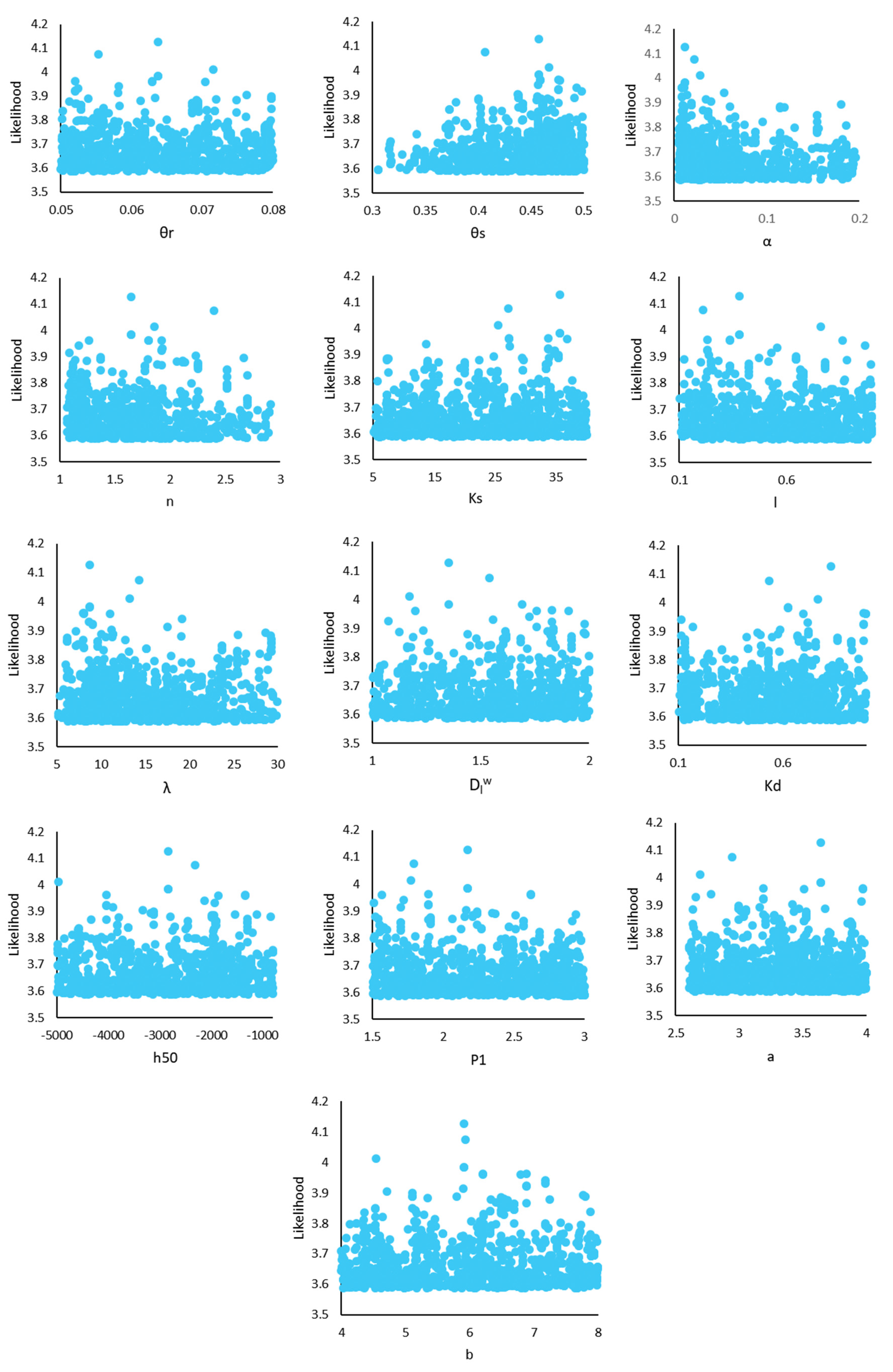
The Generalized Likelihood Uncertainty Estimation (GLUE) is a Bayesian theorem-based algorithm that uses prior information about the parameters and measurement data to estimate uncertainty in model parameters [38]. Estimating the posterior distribution of the parameters is attained by sampling an enormous number of parameters from the prior distribution by Monte Carlo simulations [39]. Then, the generated parameter sets’ performances are evaluated by the likelihood function. The uncertainty estimated by GLUE considers all sources of uncertainty, including input, structure, and parameter uncertainties. The calculated value by the likelihood regarding the parameter sets reflects all sources of error with the model [40]. In the recent decade, the GLUE algorithm has received attention in agro-hydrological studies. Li et al., 2018 have proved that the calibrated DSSAT-CERES based on the GLUE method could accurately reproduce leaf area index, above-ground biomass, grain yield, and above-ground nitrogen of winter wheat in the Beijing area [41]. Sun et al., 2016 successfully calibrated the parameters of the RZWQM-DSSAT (RZWQM2) model for simulating crop growth and transporting water and nitrogen in a wheat-maize cropping system using the GLUE method with some adjustments in its likelihood function [42]. Their uncertainty analysis results declared that the parameters related to soil-saturated hydraulic conductivity, nitrogen nitrification and denitrification, and urea hydrolysis were the most effective ones in simulating crop yield components. Sheng et al., 2019 compared two Bayesian theorem-based algorithms of GLUE and DREAM for estimating parameters associated with cultivars in the APSIM-maize model. They found similar performance between GLUE and DREAM algorithms [43]. Uncertainty assessment of the SWAP model for simulating soil water content (SWC) at a field scale using the GLUE method has been explored by Shafiei et al., 2014 [40]. Their results revealed that the predictive uncertainty in simulating SWC was low, which proved the good performance of the SWAP model in dry regions at the field scale.
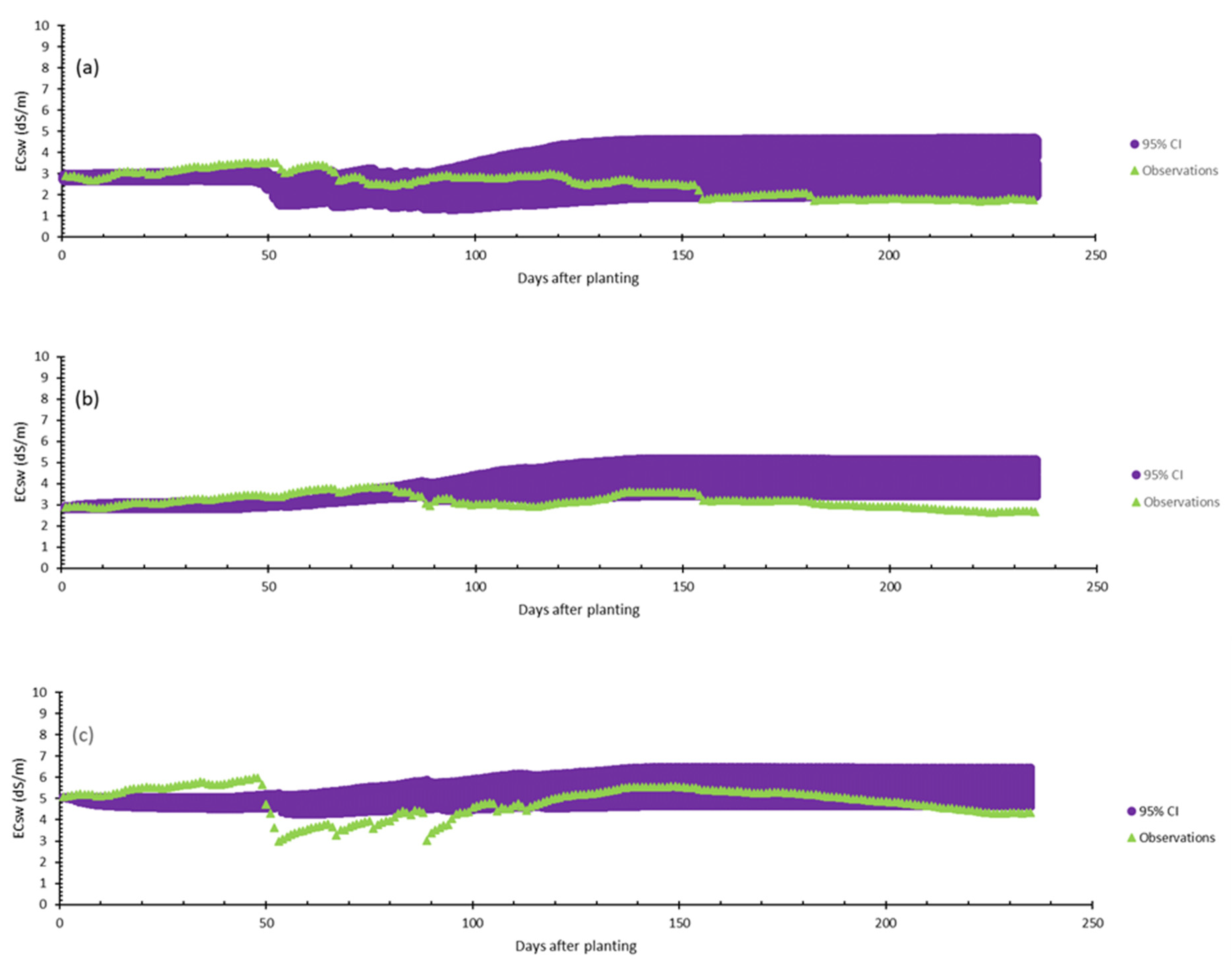
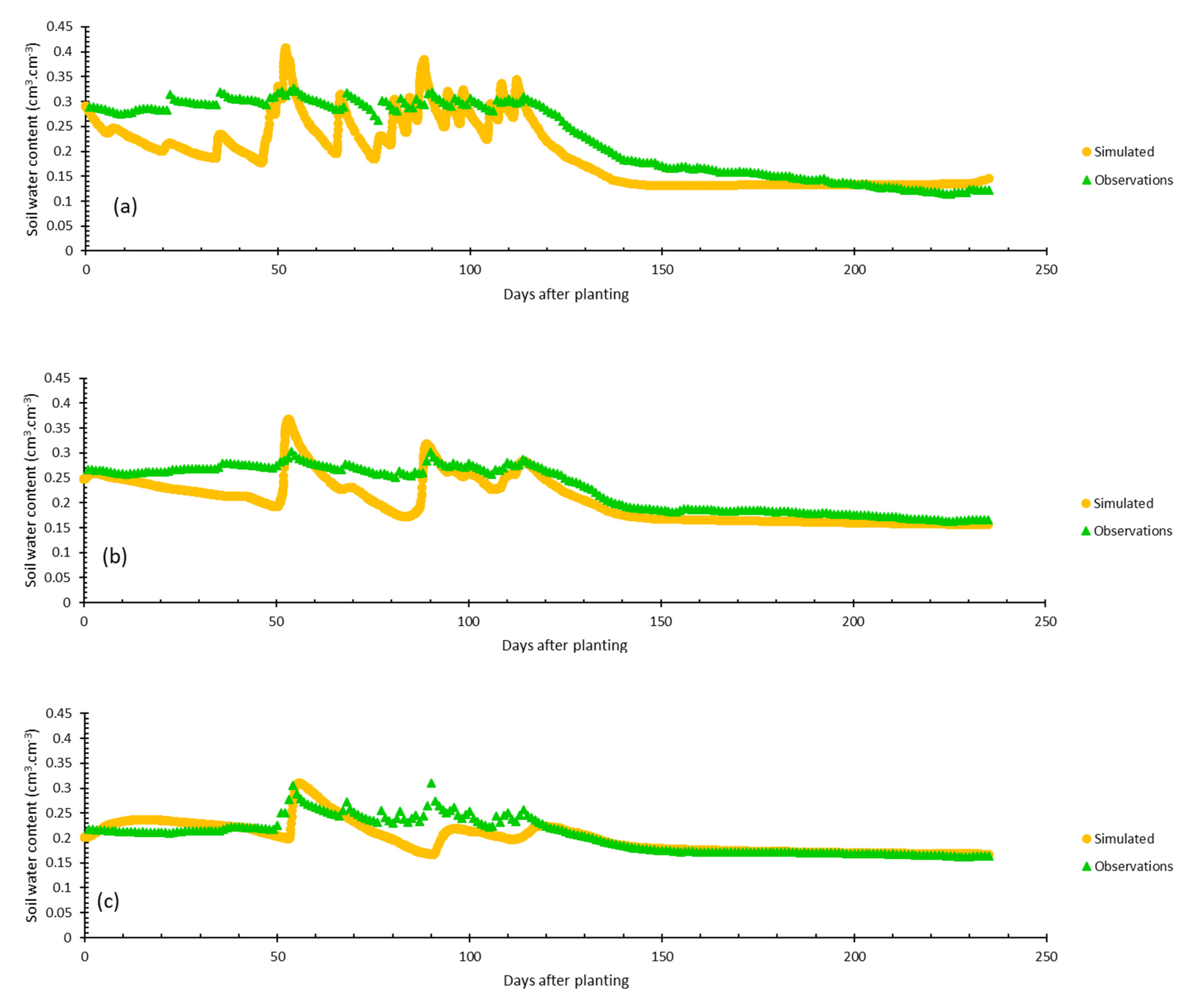
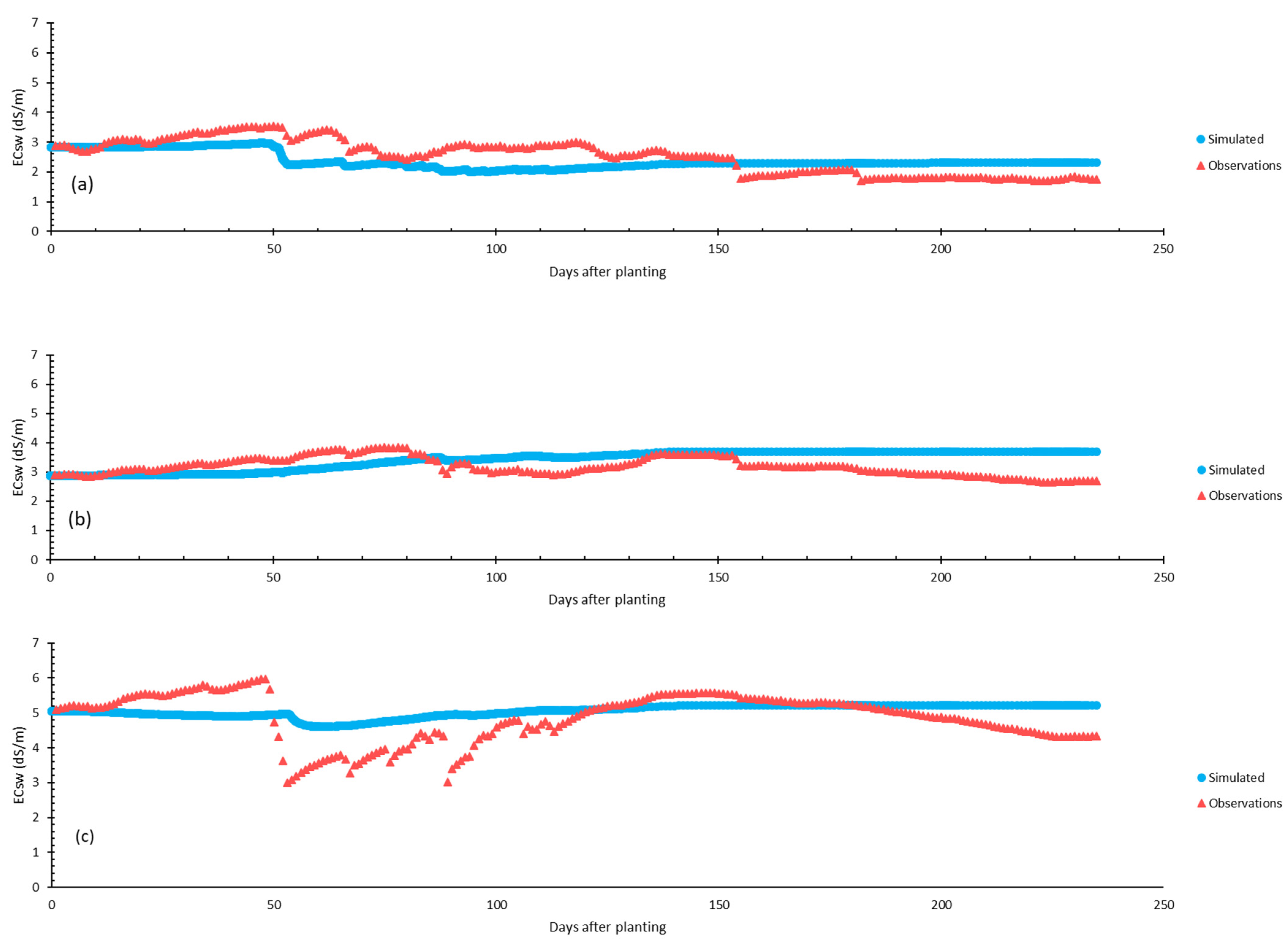
To date, few studies have focused on Bayesian calibration and uncertainty analysis of HYDRUS-1D, explicitly using the GLUE method for simulating soil salt dynamics under sprinkler irrigation systems at field scale. Thus, the main objective of this research was to calibrate and assess the uncertainty of the HYDRUS-1D model for simulating transient conditions of salts in the corn root zone in western Kansas based on the GLUE method.

2. Materials and Methods

2.1. Site Description

Field experiments were conducted at Kansas State University, Southwest Research-Extension Center, near Garden City, Kansas. The geographical coordinates of the experimental field are 38°01′20.87″ N, 100°49′26.95″ W, and the altitude of the area is 887 m above sea level. According to the long-term weather data of Garden City, KS, the total annual precipitation and evapotranspiration are 477 and 1810 mm, respectively. The well-drained Ulysses silt loam was the predominant soil type [44]. The physical characteristics of the soil (fine-silty, mixed, mesic Aridic Haplustoll) are presented in Table 1. In addition, the soil pH was 8.3, and the experimental area has 170 days frost-free period [44,45]. The electrical conductivity of irrigation water was 1.2 dS/m and its sodium adsorption ratio (SAR) was 2.6 (meq/L)0.5. Therefore, the irrigation water chemical characteristics were categorized as C1-S1 in the USSL classification (Table 2). A four-span linear move irrigation system (model 8000, Valmont Corp., Valley, NE, USA) was used to implement irrigation for the aims of the study, and the plots’ sizes of the study were 13.7 m × 27.4 m.

2.2. Data Collection and Management

The conventional corn was planted on 11 May 2016, with 84,000 seeds/ha seeding rate, and harvested on 6 October 2016. The corn plant spacing was 20 cm, and the row spacing was 70 cm. The irrigation events started on 1 April 2016 and terminated on 15 September 2016. The irrigation frequency was determined according to soil water content readings based on 50% soil water depletion. The TDRs (CS655 manufactured by Campbell Scientific, Logan, UT, USA) with 12 cm rods were installed at 16, 46, and 76 cm of soil depth, respectively, to monitor the volumetric soil water content (SWC) and soil salinity (ECsw) [46,47] at the same time during and out of the growing season. The sensors were installed for three different plots with the same installation depths. The SWC and ECsw were collected every 30 min using the Campbell Scientific data loggers. The observational data were collected for 235 days (11 May 2016 to 31 December 2016). The agronomic practices, including weed management and fertilizer application, were based on the recommended procedures for southwest Kansas. The initial ECsw was 2.88, 2.89, and 5.09 dS/m for 16, 46, and 76 cm soil depth, respectively. Daily meteorological data, including minimum and maximum temperature, relative humidity, solar radiation, wind speed, and precipitation, were obtained from the nearby tower of the K-State MESONET network. The FAO-Penman Monteith method was used to calculate daily evapotranspiration [48]. Daily crop evapotranspiration and precipitation during and out of the growing season are depicted in Figure 1. The 25.4 mm irrigation depth was constant for each irrigation event. In addition, crop mapping was done multiple times during the growing season to measure the leaf area index (LAI) and record crop growth stages. All of these data were used as input for atmospheric boundary conditions and observational data for calibration purposes. In addition, the SWC and ECsw data were measured during and out of the growing season to comprehend salts and SWC dynamics in the field condition. The initial soil profile water content and salinity at different depths are presented in Table 3.

2.3. HYDRUS-1D Model

The simulations were done from the planting date to the beginning of the next growing season.

2.3.1. Water Flow Modeling

To simulate the water flow in the soil, the Richards’ Equation (1) was solved numerically in HYDRUS-1D using Galerkin finite element scheme [21]:
θ t = z K h h z 1 S z , t
where θ is soil volumetric water content (L3L−3), t is time (T), z is vertical space coordinate (L), K(h) is unsaturated hydraulic conductivity function (LT−1), h is soil pressure head (L), and S(z,t) is sink term (L3L−3T−1) representing the unit volume of water removed by the crop from a unit of volume of soil per time unit.
The HYDRUS-1D model utilized the following equation to represent the relations between θ and h [49]:
θ h = θ s θ r 1 + α h n 1 1 n + θ r                   h < 0   θ s                                                                               h > 0
where θs is saturated soil volumetric water content (L3L−3), θr is residual soil volumetric water content (L3L−3), and α and n are empirical parameters.
The model used the following unsaturated soil hydraulic conductivity function [49]:
K h = K s S e l 1 1 S e n n 1 1 1 n 2                   h < 0   K s                                                                                                     h > 0
where Ks is saturated hydraulic conductivity (LT−1), l is an empirical parameter known as tortuosity parameter (dimensionless), Se is relative soil effective saturation
(Se = θ − θrs − θr)

2.3.2. Root Water Uptake

The sink term (S(z,t)) in Richards’ equation which is known as the root water uptake term as well, was calculated in the following equation (Equation (4)) to account for water and salinity stress in the multiplicative form:
S z , t =   α h , π β z T p
where the α(h, π) is water and salinity stress reduction function (dimensionless), β(z) is normalized root density distribution (L−1), Tp is potential transpiration rate (L3L−2.T−1)
The α function that accounts for the combination of water and salinity stresses has been built from the multiplication of the S-shape water stress function and threshold and slope function for salinity stress as follows [50]:
α h , π = 1 1 + h h 50 p 1 + b π a  
where h is soil pressure head (L), h50 is the pressure head at which water uptake is reduced by 50% and negligible osmotic (salinity) stress exists, and p is an empirical parameter. The π is soil salinity (dS/m), b is the slope of root water uptake reduction, and a is the root water uptake threshold to soil salinity (dS/m).
The normalized root distribution (Equation (6)) as a function of root depth is as follows:
β z = 1 ,                                                                     Z = 0 0.007 Z + 1 ,                 0 < Z < 150   c m 0 ,                                               Z > 150   c m
where z is root depth (L).
To calculate the potential transpiration (Tp), initially, the potential evapotranspiration (ETp) was calculated by the FAO Penman-Monteith equation [48]. For the next step, the potential evaporation was computed using the following equation [51]:
Ep = ET p e kLAI
where k is crop canopy radiation attenuation coefficient (dimensionless), which is usually taken as 0.4, and LAI is leaf area index. Then the potential transpiration (L T−1) was estimated by:
T p = ET p E p

2.3.3. Solute Transport

The advection-dispersion equation (ADE) was solved numerically by HYDRUS-1D using the Galerkin finite elements scheme for space weighting and the Crank-Nicholson scheme for time weighting [52]:
c t + ρ 0 θ   s t = D e 2 c 2 z q w θ c z  
where c is liquid phase (dissolved) solute concentration (ML−3), s is solid phase concentration (MM−1), t is time (T), θ is volumetric soil water content (L3L−3), De is effective dispersion coefficient (L2T−1), qw is soil water flux (L3L−2T−1), z is vertical coordinates (L).
The effective dispersion coefficient accounts for diffusion and hydrodynamic dispersion coefficients [52]:
D e = D l s + D lh  
D lh = λ q w θ  
D l s = θ 7 3 θ s 2 D l   w
where Dls is soil effective diffusion coefficient (L2T−1), Dlh is coefficient of hydrodynamic dispersion (L2T−1), λ is known as dispersivity [L], θs is saturated volumetric water content, and Dlw is diffusion coefficient in free water (L2T−1).
In this research, adsorption of salts was assumed to be the linear equilibrium (instantaneous):
s = K d c
where Kd is known as the distribution coefficient or adsorption isotherm coefficient (L3M−1).

2.4. The HYDRUS-1D Model Setup

The soil salinity of the corn root zone irrigated with saline water was simulated using the HYDRUS-1D model. The first 200 cm layer of the soil profile was considered for simulations. One soil material and layer were considered because the soil profile at the experimental field had a relatively uniform texture to 240 cm deep. The simulations were done on a daily basis for 235 days (from 11 May 2016, to 31 December 2016). The Van Genuchten-Mualem (Equations (2) and (3)) hydraulic model was chosen to perform the water flow simulation and describe the unsaturated soil hydraulic properties. The initial arbitrary values of the water flow parameters were obtained from the HYDRUS-1D library for the silt loam soil. The atmospheric boundary condition with the surface layer was chosen as the study was conducted in the field. The free drainage boundary condition was used for the bottom of the soil profile. The linear equilibrium adsorption was used to imitate the adsorption process under saline irrigation conditions. The upper and bottom boundary conditions for the Advection-Dispersion equation were concentration flux and zero concentration, respectively. The root water uptake simulations were done by applying the S-Shape model as a reduction function for water stress, and simultaneously the slope and threshold salinity stress reduction function was considered in a multiplicative approach.

2.5. Uncertainty Assessment and GLUE Method

The uncertainty in water management has been illustrated as the degree of confidence (probability) in the decision-making process using simulation tools [53]. To pursue the uncertainty analysis, the GLUE method was implemented for the HYDRUS-1D model to simulate the dynamic of salts under linear move irrigation. It was assumed that the results of this study would assess the degree of confidence in using the HYDRUS-1D to explore salinity management scenarios, primarily through the leaching application process. Therefore, the following sets of parameters were subjected to uncertainty analysis:
  • Water flow simulation parameters: [θr, θs, α, n, Ks, l]
  • Solute transport parameters: [λ, Dlw, Kd]
  • Root water uptake = [a, b, h50, P1]
The existing values of parameters in the slope-threshold method (salinity stress) in the literature [54,55] are very general. Thus, they need to be determined for a specific location with its particular soil and weather characteristics. Because of this reason, the a and b were subjected to calibration and uncertainty analysis.
To successfully perform uncertainty analysis using the GLUE method, a subjective threshold for likelihood values should be assigned to find behavioral parameter sets. Those parameter sets found behavioral were used for uncertainty analysis. Furthermore, another prevalent issue in HYDRUS-1D simulations is the non-convergence of the model outputs for some parameter sets. On that account, all of those parameter sets that resulted in model non-convergence were eliminated during computations. The last elimination procedure was called the screening operation.
The following steps were used to apply the GLUE algorithm [41]:
1.
The prior distributions of parameters were identified based on the HYDRUS-1D model library and existing values in the literature (Table 4). The priors were considered uniformly distributed.
2.
The parameters’ ranges were randomly sampled n times based on the Monte Carlo approach in RStudio 1.41717 environment.
3.
The HYDRUS-1D model was run in the RStudio environment for each parameter set already sampled.
4.
The likelihood values were calculated using inverse error variance as the likelihood function:
L θ j | O = i = 1 n O i y i θ j 2 n 2 1
where θj is jth parameter set, Oi is ith observation, y is the model output n is the number of observations.
5.
The threshold for likelihood values for behavioral parameter sets was specified. In this study, 10% of successful parameters after screening operation were used for uncertainty analysis.
6.
The probability of each parameter set was computed using the following equation:
p θ j = L θ j | O J = 1 n L θ j | O
where p(θj) is the probability (likelihood weight) of the jth parameter set, n is the number of parameters’ sets, and L(θj|O) is the value of the likelihood of the jth parameter set.
7.
The posterior distributions of the parameters and statistics were constructed. The empirical posterior distributions of parameters were achieved by pairs of parameters’ sets (θj) and their corresponding probabilities. Then, by using the following equations, the mean and variance of the parameters were calculated:
μ post = j = 1 n p θ i θ i
Var post = j = 1 n p θ i ( θ i μ post ) 2
where μpost and Varpost are the mean and variance of the posterior distribution of the parameters.
8.
For the final step, the simulated values of soil water salinity by the HYDRUS-1D model were sorted based on the corresponding probabilities to create a cumulative distribution function of model outputs (predictive uncertainty). Then 95% confidence intervals for model outputs were retrieved [40].
The HYDRUS-1D model was run 126,000 times in the R environment to implement the GLUE algorithm and achieve this study’s goals. After the screening procedure and applying threshold values for exploring behavioral parameters sets, the 1000 sets of parameters remained for uncertainty analysis.
The 50% and 97.5% quantiles of the posterior distributions of the parameters were considered as calibrated values of the parameters for investigating the model performance in terms of simulating soil water content and ECsw. In addition, the single parameter set that resulted in the highest likelihood value was used as an alternative scenario for the calibration of the model.

2.6. Evaluation of the Model Performance

Three statistical indices were used to evaluate the model performance: root mean square error (RMSE), normalized root mean square error (NRMSE), and coefficient of determination (R2):
RMSE = 1 n i = 1 n M i S i 2
NRMSE = RMSE M ¯
R 2 = ( i = 1 n ( M i M ¯ ) ( S i S ¯ ) ) i = 1 n M i M ¯ 2 i = 1 n S i S ¯ 2
where Mi, Si, and M ¯ are measured value, simulated value, and the average value of measurements. The R2 values close to 1 indicate the good performance model. The NRMSE ranges of <10%, 10–20%, 20–30%, and >30% categorize the model performance as excellent, good, fair, and poor.

3. Results and Discussion

In this section, the uncertainty in the model parameters and simulated outputs were initially quantified and then presented and discussed. This information would provide interesting clues to find roots of error in simulating soil salinity during and out of corn growing season irrigated with saline water under a linear move irrigation system. Afterward, the results of the performance analysis of the model calibrated with posterior values of the parameters using the GLUE algorithm are presented and discussed.

3.1. Parameters Uncertainty

The posterior distributions of the parameters indicate different levels of uncertainty in derived (SD) parameters using the GLUE algorithm. Comparing the statistical indices, specifically standard deviations associated with prior and posterior distributions (Table 4 and Table 5) of the parameters reveals that the algorithm was able to reduce the uncertainty of a certain number of parameters. By using observational ECsw data, the algorithm was able to estimate the θs, n, and α as 26, 22, and 8% reduction was obtained in their posterior standard deviation values compared to their priors. Likewise, the posterior SD values of λ and Kd parameters of solute transport parameters were reduced by 16 and 15% compared with their corresponding prior values. Furthermore, the reduction in SD values of posterior distributions root water uptake reduction function for salinity stresses indicated a lower level of uncertainty remaining in these parameters (a and b). Contrastingly, estimations of the rest of the parameters were accomplished with lower confidence (higher uncertainty) as there was no considerable difference between the SD values of their posteriors and priors. The histograms of the parameters’ posterior distributions are presented in Figure 2, Figure 3 and Figure 4. The x-axis of the graphs was considered equal to the prior distribution of the parameters to compare posteriors and priors. Among the water flow simulating parameters, the skewed and peaked posterior distributions have been observed for θs, α, and n. It indicates the lower level of uncertainty remained in these parameters after implementing the GLUE algorithm for the HYDRUS-1D model to simulate soil salinity under irrigation with saline water using a linear move irrigation system. The posteriors of θr, Ks, and l were slightly changed from their priors as they uniformly covered the upper and lower bounds of the prior distribution. Posterior distributions of solute transport parameters show (Figure 3) that the dispersivity (λ) and adsorption isotherm coefficient (Kd) approximately follow a normal distribution, indicating a reduction in the uncertainty of their estimations.
Nevertheless, the posterior distribution of the diffusion coefficient (Dlw) was not noticeably different from its prior distribution. This could be because the diffusivity contribution to the solute transport procedure for saline water irrigation conditions was trivial compared with advection and hydrodynamic dispersion. In addition, the posterior distribution of the root water uptake threshold (a) was picked and concentrated around the median. However, the other parameters did not significantly change from their priors, indicating a higher level of uncertainty in these parameters after derivation by the GLUE algorithm [23]. This is presumably because of the scale of the study, as our experimental field had plots 13.7 m × 27.4 m dimensions. Studies conducted at the field scale can potentially increase the uncertainty in observational data due to several phenomena, such as uniformity distribution of irrigation applications, preferential flows as a consequence of compaction or shrinkage of dry soil before irrigation events, and soil water redistribution in the soil. On the other hand, the results showed that threshold reduction in root water uptake, which is presented generally in the literature, could be adequately derived for a specific location by the GLUE algorithm. This threshold value could be used as a guideline for leaching requirement specifications and designing irrigation systems. To compare the computed value of root water uptake threshold with the existing values in the literature [54], The value should be divided by 2 because the HYDRUS-1D model uses the values of electrical conductivity of soil water (ECsw). The values in the literature are presented as the electrical conductivity of soil-saturated paste extract (ECe). Our results found ECsw = 3.324 dS/m or ECe = 1.662 dS/m, which was very close to the ones reported by Mass and Hoffman, 1977 (ECe = 1.7 dS/m)—[54]. The relative sensitivity of the parameters can be analyzed by comparing the CV values of the prior and posterior distribution of the parameters. The α, a, and b were the three most sensitive parameters. In contrast, the three l, h50, and P1 were the least sensitive parameters, respectively, for simulating soil salinity at the corn root zone at the field scale. The scatter plots of likelihood values of behavioral parameters’ sets related to water flow, solute transport, and root water uptake processes are presented in Figure 5 to explore further aspects in identifying the parameters. These plots demonstrate that the single optimum parameter set is identifiable because the parameter set’s corresponding likelihood value was significantly higher in the parameters’ response surface than the majority of the other parameter’s values. The optimum water flow simulation parameters sets are θr = 0.0637, θs = 0.4575, α = 0.0119, Ks = 35.71, n = 1.647, and l = 0.3797. The optimum solute transport and root water uptake parameters are λ = 8.712, Dlw = 1.35, Kd = 0.83, h50 = −2845, P1 = 2.17, a = 3.63, and b = 5.913. Furthermore, based on Figure 5, ranges with higher probability or lower uncertainty in the parametric surface response of parameters can be identified only for θs and α. The results show that the ranges are: θs = [0.45–0.49], and α = [0.01–0.065].

3.2. Predictive Uncertainty

Analysis of the predictive uncertainty (model output uncertainty) provides additional information regarding the sources of uncertainty in model outputs and the successfulness of the GLUE algorithm in the calibration of the HYDRUS-1D model. The output uncertainty of the model based on 95% CI of behavioral parameters is depicted in Figure 6 for soil depths of 16, 46, and 76 cm. The shaded areas are the predictive uncertainty of the model, and green triangular points are observations of ECsw. The results declare that the uncertainty in the model parameters has reached the model outputs as the observational data are primarily covered in the predictive uncertainty band (shaded area). Moreover, covering the majority of the observational points by the 95% CI band show that the primary source of uncertainty in simulating ECsw of corn root zone under saline irrigation is uncertainty in the parameters’ estimations. As it is expressed in Figure 6, the predictive uncertainty band varies during the growing season (The corn was harvested 128 days after the planting date), and it is approximately constant for the out of the growing season period. This is related to the absence of irrigation or significant precipitation after the growing season and the lack of root water uptake. Thus, the only remaining factor affecting the soil water and salinity balance was substantially low evaporation (Figure 1) in such a way that it could not change the uniformity of the uncertainty band out of the growing season.
Additionally, the increase in predictive uncertainty can be inferred for the drier period of the field due to the magnification of the unsaturated condition, which increases the complexity of simulating water flow and solute transport process. The model outputs’ uncertainty band was substantially lower for the first 50 days of the growing season (the corn reached the V8 growth stage) compared to the other days. This could be because the corn was at its initial growth stages, and root water uptake did not considerably affect the soil water content and, consequently, the ECsw at the measurement depths. Increasing the output uncertainty after corn’s initial growth stages could be explained by remaining uncertainties in the root water uptake reduction parameters for water stress, as they were relatively higher than the other parameters, and the 95% CI band covered the observational points. Moreover, the predictive uncertainty band only covers a portion of the observational points for ECsw simulations at 76 cm soil depth, which could be related to existing errors in boundary conditions. Due to the scale of the study, the irrigation application efficiency of linear move irrigation systems could sometimes vary due to the prevailing windy conditions of western Kansas. It is probable that during some of the irrigation events, the unexpected wind changed the amount of water received by the soil, which consequently caused errors in the boundary condition of the study.

3.3. The HYDRUS-1D Model Performance

The performance of the calibrated HYDRUS-1D model based on 50 and 97.5% quantiles of parameters posterior distributions (Table 5) and optimum parameters set based on likelihood scatterplots (Figure 5) are presented in Table 6. The model’s excellent accuracy has been observed in simulating soil water content and ECsw during and out of the corn growing season for all three series of parameters.
The obtained RMSE values for simulating SWC were from 0.0006 and 0.008 cm3cm−3 for parameters’ sets based on the 50% and 97.5% quantiles of parameters posteriors and likelihood scatterplots used as calibrated values. The NRMSEs for simulating SWC were from 0.003 to 0.01. The highest accuracy of the model was detected for simulating SWC at 76 cm depth during and out of the growing season. In addition, good adequacy of the model was noticed based on R2 values between simulated and measured SWCs. The calibrated HYDRUS-1D model based on 50% quantiles posteriors resulted in the highest accuracy of the model for simulating SWC compared with the other two series of calibration values.
Furthermore, the highest adequacy of the model was obtained for optimum parameters’ values based on likelihood scatterplots to simulate SWC. The overall performance of the calibrated model, based on all three calibration scenarios, was excellent based on statistical indices (Table 6). It has been detected that RMSE values for predicted ECsw were from 0.29 to 0.42 dS/m and 0.16 to 0.46 dS/m for the calibrated model based on 50% and 97.5% quantiles of the parameters’ posteriors. Moreover, RMSE values were from 0.23 to 0.53 dS/m for simulating ECsw using calibrated model based on optimum values obtained from scatterplots of the likelihood values. The performance results show that the adequacy of the model for simulating ECsw was not as satisfying as SWC simulations during and out of the corn growing season in our study region. The R2 values were from 0.13 to 0.60 for both parameters’ sets. The highest adequacy of the model for ECs predictions was observed at 16 cm soil depth for calibrated model based on likelihood values, and the lowest one was noticed for ECsw simulations at 46 cm soil depth for calibrated model based on 97.5% of parameters posterior distributions.
The results of this study indicated that using 50% quantiles of parameters posterior distributions could be introduced as acceptable calibration results for implementation of the GLUE algorithm for the HYDRUS-1D model to simulate salinity of corn root zone at field scale under linear move irrigation system. The time series of simulated soil water content and ECsw, along with observational for different soil depths, are presented in Figure 7 and Figure 8 to obtain further details on the performance of the calibrated model based on 50% quantiles of parameters posteriors. The good performance of the model during the corn growing season and the excellent performance of the model for simulating SWC was observed for all three soil depths. The model outputs follow the observational SWC data trend.
Similar performance of the model was observed for ECsw simulation. The discrepancies between observations and simulated were not noticeable for salinity simulations. However, some noticeable deviations were detected between simulated and observed ECsw values at 76 cm soil depth, which was expected as another source of uncertainty detected for this soil depth in the analysis of the model predictive uncertainties.

4. Conclusions

A study was conducted to investigate calibration and the uncertainty in parameters and outputs of the HYDRUS-1D model to simulate soil salinity of corn root zone under irrigation with saline water using a linear move irrigation system. In this research, the generalized likelihood uncertainty estimation (GLUE) algorithm was implemented for the HYDRUS-1D model in the R environment to achieve the goals of the study. The results have found a lower level of uncertainty in θs, n, and α among the soil water flow simulations parameters, adsorption isotherm coefficient (Kd) and dispersivity (λ) among the solute transport parameters, and threshold (a) and slope (b) parameters of root water uptake reduction function for salinity stress compare to uncertainty in the other parameters. This study detected a minor contribution of the coefficient of diffusion in the solute transport process at the field scale compared to advection and hydrodynamic dispersion because its posterior distribution was not noticeably different from its corresponding priors. The mean value of the posterior distribution of the root water uptake threshold to salinity was 1.662 dS/m, which was close to the value reported by Mass and Hoffman, 1977 [41] for corn (ECe = 1.7 dS/m). The relative sensitivity analysis of parameters has revealed α and P1 as the most sensitive and least sensitive parameters, respectively. Predictive uncertainty analysis showed that the uncertainty in the HYDRUS-1D parameters is the main source of uncertainty in the model outputs. In addition, it was illustrated that uncertainty in model outputs for simulating ECsw was relatively lower in the initial growth stages (emergence to V8) of corn compared to the other growth stages and out of the growing season. The model was able to successfully simulate the soil water content and electrical conductivity of soil water (ECsw) with calibrated parameters using 50% quantiles of the parameters’ posterior distributions. The ranges of NRMSE values were 0.003 to 0.01 for simulating soil water content and 0.09 to 0.11 for simulating ECsw, which specify the excellent performance of the calibrated model based on posterior distributions of parameters. The results of this study have proved the reliability of the GLUE algorithm to explore uncertainty analysis of the HYDRUS-1D model and its calibration for reproducing soil salinity of corn root zone under saline water irrigation at field scale under linear move sprinkle irrigation system.

Author Contributions

Conceptualization, F.M. and B.G.; methodology, F.M., A.M., M.C.G. and B.G.; supervision, A.M., J.A. and B.G.; software, F.M. and J.A.; investigation, F.M., data curation, J.A.; resources, J.A. and H.A., writing-the original draft preparation, F.M., writing-review and editing, F.M., A.M. and J.A. All authors have read and agreed to the published version of the manuscript.

Funding

The APC was funded by Kansas State University and USDA-ARS, Ogallala Aquifer Program.

Institutional Review Board Statement

Not applicable.

Informed Consent Statement

Not applicable.

Data Availability Statement

The data could be available by requesting Dr. J.A.

Acknowledgments

The group of authors would like to thank Kansas State University for financially supporting the APC for this study. Special thanks to Mojtaba Shafiei, the astonishing alumni of Ferdowsi University of Mashhad for being pioneer of implementing Bayesian statistics concepts in the department of water science and engineering.

Conflicts of Interest

The authors declare no conflict of interest.

References

  1. Skaggs, T.H.; Anderson, R.G.; Corwin, D.L.; Suarez, D.L. Analytical steady-state solutions for water-limited cropping systems using saline irrigation water. Water Resour. Res. 2014, 50, 9656–9674. [Google Scholar] [CrossRef]
  2. Bradford, S.; Letey, J. Cyclic and blending strategies for using nonsaline and saline waters for irrigation. Irrig. Sci. 1992, 13, 123–128. [Google Scholar] [CrossRef]
  3. Rhoades, J.D. Use of saline drainage water for irrigation. Agric. Drain. 1999, 38, 615–657. [Google Scholar]
  4. Sharma, D.P.; Rao, K. Strategy for long term use of saline drainage water for irrigation in semi-arid regions. Soil Tillage Res. 1998, 48, 287–295. [Google Scholar] [CrossRef]
  5. Mendoza-Espinosa, L.G.; Burgess, J.E.; Daesslé, L.; Villada-Canela, M. Reclaimed water for the irrigation of vineyards: Mexico and South Africa as case studies. Sustain. Cities Soc. 2019, 51, 101769. [Google Scholar] [CrossRef]
  6. Kramer, I.; Bayer, Y.; Mau, Y. The sustainability of treated wastewater irrigation: The impact of hysteresis on saturated soil hydraulic conductivity. Water Resour. Res. 2022, 58, e2021WR031307. [Google Scholar] [CrossRef]
  7. Sheng, F.; Xiuling, C. Using shallow saline groundwater for irrigation and regulating for soil salt-water regime. Irrig. Drain. Syst. 1997, 11, 1–14. [Google Scholar] [CrossRef]
  8. Zhang, J.; Li, K.; Gao, Y.; Feng, D.; Zheng, C.; Cao, C.; Sun, J.; Dang, H.; Hamani, A.K.M. Evaluation of saline water irrigation on cotton growth and yield using the AquaCrop crop simulation model. Agric. Water Manag. 2022, 261, 107355. [Google Scholar] [CrossRef]
  9. Singh, A. Soil salinization management for sustainable development: A review. J. Environ. Manag. 2021, 277, 111383. [Google Scholar] [CrossRef]
  10. Fathizad, H.; Ali Hakimzadeh Ardakani, M.; Sodaiezadeh, H.; Kerry, R.; Taghizadeh-Mehrjardi, R. Investigation of the spatial and temporal variation of soil salinity using random forests in the central desert of Iran. Geoderma 2020, 365, 114233. [Google Scholar] [CrossRef]
  11. Mostafazadeh-Fard, B.; Mansouri, H.; Mousavi, S.-F.; Feizi, M. Effects of Different Levels of Irrigation Water Salinity and Leaching on Yield and Yield Components of Wheat in an Arid Region. J. Irrig. Drain. Eng. 2009, 135, 32–38. [Google Scholar] [CrossRef]
  12. Kang, Y.; Chen, M.; Wan, S. Effects of drip irrigation with saline water on waxy maize (Zea mays L. var. ceratina Kulesh) in North China Plain. Agric. Water Manag. 2010, 97, 1303–1309. [Google Scholar] [CrossRef]
  13. Li, D.; Wan, S.; Li, X.; Kang, Y.; Han, X. Effect of water-salt regulation drip irrigation with saline water on tomato quality in an arid region. Agric. Water Manag. 2022, 261, 107347. [Google Scholar] [CrossRef]
  14. Corwin, D.L.; Waggoner, B.L. TETrans: A user-friendly, functional model of solute transport. Water Sci. Technol. 1991, 24, 57–65. [Google Scholar] [CrossRef]
  15. Oosterbaan, R.J. SALTMOD: Description of Principles, User Manual, and Examples of Application, Version 1.1; ILRI: Wageningen, The Netherlands, 2001. [Google Scholar]
  16. Shahrokhnia, H.; Wu, L. SALEACH: A new web-based soil salinity leaching model for improved irrigation management. Agric. Water Manag. 2021, 252, 106905. [Google Scholar] [CrossRef]
  17. Liu, Y.; Zhu, Y.; Mao, W.; Sun, G.; Han, X.; Wu, J.; Yang, J. Development and Application of a Water and Salt Balance Model for Well-Canal Conjunctive Irrigation in Semiarid Areas with Shallow Water Tables. Agriculture 2022, 12, 399. [Google Scholar] [CrossRef]
  18. Corwin, D.L.; Waggoner, B.L. TETRANS: Solute Transport Modeling Software User’s Guide; Report 121. USDA-ARS; U.S. Salinity Laboratory: Riverside, CA, USA, 1990.
  19. Chang, X.; Gao, Z.; Wang, S.; Chen, H. Modelling long-term soil salinity dynamics using SaltMod in Hetao Irrigation District, China. Comput. Electron. Agric. 2019, 156, 447–458. [Google Scholar] [CrossRef]
  20. Letey, J.; Hoffman, G.J.; Hopmans, J.W.; Grattan, S.R.; Suarez, D.; Corwin, D.L.; Oster, J.D.; Wu, L.; Amrhein, C. Evaluation of soil salinity leaching requirement guidelines. Agric. Water Manag. 2011, 98, 502–506. [Google Scholar] [CrossRef] [Green Version]
  21. Simunek, J.; Van Genuchten, M.T.; Sejna, M. The HYDRUS-1D software package for simulating the one-dimensional movement of water, heat, and multiple solutes in variably-saturated media. Univ. Calif.-Riverside Res. Rep. 2005, 3, 240. [Google Scholar]
  22. Liu, B.; Wang, S.; Liu, X.; Sun, H. Evaluating soil water and salt transport in response to varied rainfall events and hydrological years under brackish water irrigation in the North China Plain. Geoderma 2022, 422, 115954. [Google Scholar] [CrossRef]
  23. Noshadi, M.; Fahandej-Saadi, S.; Sepaskhah, A.R. Application of SALTMED and HYDRUS-1D models for simulations of soil water content and soil salinity in controlled groundwater depth. J. Arid Land 2020, 12, 447–461. [Google Scholar] [CrossRef]
  24. Kanzari, S.; Ben Nouna, B.; Ben Mariem, S.; Rezig, M. Hydrus-1D model calibration and validation in various field conditions for simulating water flow and salts transport in a semi-arid region of Tunisia. Sustain. Environ. Res. 2018, 28, 350–356. [Google Scholar] [CrossRef]
  25. Shaygan, M.; Baumgartl, T.; Arnold, S.; Reading, L.P. The effect of soil physical amendments on reclamation of a saline-sodic soil: Simulation of salt leaching using HYDRUS-1D. Soil Res. 2018, 56, 829–845. [Google Scholar] [CrossRef]
  26. Ramos, T.B.; Šimůnek, J.; Gonçalves, M.C.; Martins, J.C.; Prazeres, A.; Castanheira, N.L.; Pereira, L.S. Field evaluation of a multicomponent solute transport model in soils irrigated with saline waters. J. Hydrol. 2011, 407, 129–144. [Google Scholar] [CrossRef]
  27. Askri, B.; Ahmed, A.T.; Abichou, T.; Bouhlila, R. Effects of shallow water table, salinity and frequency of irrigation water on the date palm water use. J. Hydrol. 2014, 513, 81–90. [Google Scholar] [CrossRef]
  28. Skaggs, T.H.; Shouse, P.J.; Poss, J.A. Irrigating Forage Crops with Saline Waters: 2. Modeling Root Uptake and Drainage. Vadose Zone J. 2006, 5, 824–837. [Google Scholar] [CrossRef]
  29. Ali, A.; Bennett, J.M.; Biggs, A.A.J.; Marchuk, A.; Ghahramani, A. Assessing the hydraulic reduction performance of HYDRUS-1D for application of alkaline irrigation in variably-saturated soils: Validation of pH driven hydraulic reduction scaling factors. Agric. Water Manag. 2021, 256, 107101. [Google Scholar] [CrossRef]
  30. Phogat, V.; Yadav, A.K.; Malik, R.S.; Kumar, S.; Cox, J. Simulation of salt and water movement and estimation of water productivity of rice crop irrigated with saline water. Paddy Water Environ. 2010, 8, 333–346. [Google Scholar] [CrossRef]
  31. He, J.; Jones, J.W.; Graham, W.D.; Dukes, M.D. Influence of likelihood function choice for estimating crop model parameters using the generalized likelihood uncertainty estimation method. Agric. Syst. 2010, 103, 256–264. [Google Scholar] [CrossRef]
  32. Vrugt, J.A.; Gupta, H.V.; Bouten, W.; Sorooshian, S. A Shuffled Complex Evolution Metropolis algorithm for optimization and uncertainty assessment of hydrologic model parameters. Water Resour. Res. 2003, 39. [Google Scholar] [CrossRef] [Green Version]
  33. Braak, C.J.F. Ter A Markov Chain Monte Carlo version of the genetic algorithm Differential Evolution: Easy Bayesian computing for real parameter spaces. Stat. Comput. 2006, 16, 239–249. [Google Scholar] [CrossRef]
  34. Vrugt, J.A.; Ter Braak, C.J.F.; Diks, C.G.H.; Robinson, B.A.; Hyman, J.M.; Higdon, D. Accelerating Markov chain Monte Carlo simulation by differential evolution with self-adaptive randomized subspace sampling. Int. J. Nonlinear Sci. Numer. Simul. 2009, 10, 273–290. [Google Scholar] [CrossRef]
  35. Zhang, J.; Vrugt, J.A.; Shi, X.; Lin, G.; Wu, L.; Zeng, L. Improving Simulation Efficiency of MCMC for Inverse Modeling of Hydrologic Systems With a Kalman-Inspired Proposal Distribution. Water Resour. Res. 2020, 56, e2019WR025474. [Google Scholar] [CrossRef] [Green Version]
  36. Laloy, E.; Vrugt, J.A. High-dimensional posterior exploration of hydrologic models using multiple-try DREAM (ZS) and high-performance computing. Water Resour. Res. 2012, 48. [Google Scholar] [CrossRef] [Green Version]
  37. Vrugt, J.A.; Ter Braak, C.J.F. DREAM (D): An adaptive Markov Chain Monte Carlo simulation algorithm to solve discrete, noncontinuous, and combinatorial posterior parameter estimation problems. Hydrol. Earth Syst. Sci. 2011, 15, 3701–3713. [Google Scholar] [CrossRef] [Green Version]
  38. Beven, K.; Binley, A. The future of distributed models: Model calibration and uncertainty prediction. Hydrol. Process. 1992, 6, 279–298. [Google Scholar] [CrossRef]
  39. Makowski, D.; Wallach, D.; Tremblay, M. Using a Bayesian approach to parameter estimation; comparison of the GLUE and MCMC methods. Agronomie 2002, 22, 191–203. [Google Scholar] [CrossRef]
  40. Shafiei, M.; Ghahraman, B.; Saghafian, B.; Davary, K.; Pande, S.; Vazifedoust, M. Uncertainty assessment of the agro-hydrological SWAP model application at field scale: A case study in a dry region. Agric. Water Manag. 2014, 146, 324–334. [Google Scholar] [CrossRef]
  41. Li, Z.; He, J.; Xu, X.; Jin, X.; Huang, W.; Clark, B.; Yang, G.; Li, Z. Estimating genetic parameters of DSSAT-CERES model with the GLUE method for winter wheat (Triticum aestivum L.) production. Comput. Electron. Agric. 2018, 154, 213–221. [Google Scholar] [CrossRef] [Green Version]
  42. Sun, M.; Zhang, X.; Huo, Z.; Feng, S.; Huang, G.; Mao, X. Uncertainty and sensitivity assessments of an agricultural–hydrological model (RZWQM2) using the GLUE method. J. Hydrol. 2016, 534, 19–30. [Google Scholar] [CrossRef]
  43. Sheng, M.; Liu, J.; Zhu, A.-X.; Rossiter, D.G.; Liu, H.; Liu, Z.; Zhu, L. Comparison of GLUE and DREAM for the estimation of cultivar parameters in the APSIM-maize model. Agric. For. Meteorol. 2019, 278, 107659. [Google Scholar] [CrossRef]
  44. Klocke, N.L.; Currie, R.S.; Tomsicek, D.J.; Koehn, J. Corn yield response to deficit irrigation. Trans. ASABE 2011, 54, 931–940. [Google Scholar] [CrossRef]
  45. Araya, A.; Kisekka, I.; Gowda, P.H.; Prasad, P.V.V. Grain sorghum production functions under different irrigation capacities. Agric. Water Manag. 2018, 203, 261–271. [Google Scholar] [CrossRef]
  46. Helalia, S.A.; Anderson, R.G.; Skaggs, T.H.; Jenerette, G.D.; Wang, D.; Šimůnek, J. Impact of Drought and Changing Water Sources on Water Use and Soil Salinity of Almond and Pistachio Orchards: 1. Observations. Soil Syst. 2021, 5, 50. [Google Scholar] [CrossRef]
  47. Helalia, S.A.; Anderson, R.G.; Skaggs, T.H.; Šimůnek, J. Impact of Drought and Changing Water Sources on Water Use and Soil Salinity of Almond and Pistachio Orchards: 2. Modeling. Soil Syst. 2021, 5, 58. [Google Scholar] [CrossRef]
  48. Allen, R.G.; Pereira, L.S.; Raes, D.; Smith, M. Crop evapotranspiration-Guidelines for computing crop water requirements-FAO Irrigation and drainage paper 56. Fao Rome 1998, 300, D05109. [Google Scholar]
  49. Van Genuchten, M.T. A closed-form equation for predicting the hydraulic conductivity of unsaturated soils. Soil Sci. Soc. Am. J. 1980, 44, 892–898. [Google Scholar] [CrossRef] [Green Version]
  50. Van Genuchten, M.T. A Numerical Model for Water and Solute Movernent 1987. Available online: https://www.pc-progress.com/Documents/RVGenugten/M1987,vG,%20Worm%20USSL%20report.pdf (accessed on 9 November 2022).
  51. Ritchie, J.T. Model for predicting evaporation from a row crop with incomplete cover. Water Resour. Res. 1972, 8, 1204–1213. [Google Scholar] [CrossRef] [Green Version]
  52. Radcliffe, D.E.; Simunek, J. Soil Physics with HYDRUS: Modeling and Applications; CRC Press: Boca Raton, FL, USA, 2018; ISBN 1420073818. [Google Scholar]
  53. Klauer, B.; Brown, J.D. Conceptualising imperfect knowledge in public decision-making: Ignorance, uncertainty, error and risk situations. Environ. Res. Eng. Manag. 2004, 1, 124–128. [Google Scholar]
  54. Maas, E.V.; Hoffman, G.J. Crop salt tolerance—Current assessment. J. Irrig. Drain. Div. 1977, 103, 115–134. [Google Scholar] [CrossRef]
  55. Grieve, C.M.; Grattan, S.R.; Maas, E.V. Plant salt tolerance. ASCE Man. Rep. Eng. Pract. 2012, 71, 405–459. [Google Scholar]
Figure 1. Time series of daily crop evapotranspiration and precipitation (15 May 2016 to 31 December 2016).
Water 14 04003 g001
Figure 2. Posterior distributions of the water flow simulation parameters.
Water 14 04003 g002
Figure 3. Posterior distributions of the solute transport parameters.
Water 14 04003 g003
Figure 4. Posterior distributions of the root water uptake parameters.
Water 14 04003 g004
Figure 5. Scatterplots of likelihood values vs. the parameters of the HYDRUS-1D model.
Water 14 04003 g005
Figure 6. Predictive uncertainty of the HYDRUS-1D mode for simulating soil salinity of corn root zone at (a) 16, (b) 46 and (c) 76 cm depths.
Water 14 04003 g006
Figure 7. The simulated and observed soil water content at (a) 16, (b) 46, and (c) 76 cm soil depths.
Water 14 04003 g007
Figure 8. The simulated and observed electrical conductivity of soil water at (a) 16, (b) 46, and (c) 76 cm soil depths.
Water 14 04003 g008
Table 1. The physical characteristics of the soil at the experimental field near Garden City, KS.
Depth (cm)Soil TextureSand (%)Silt (%)Clay (%)Wilting Point (%)Field Capacity (%)Saturation (%)Bulk Density (g.cm−2)
0–240Silt loam18.555.5261533451.38
Table 2. The chemical characteristics of irrigation water.
UnitsValue
ECdS/m1.2
SAR(meq/L)0.52.64
Na+mg/L120
Ca2+mg/L58
Mg2+mg/L95
SO42−mg/L200
PO43−mg/L6.3
NO3mg/L118
K+mg/L6.1
Table 3. The initial soil water content and soil salinity.
Soil Depth (cm)Soil Water Content (cm3.cm−3)ECsw (dS/m)
0–300.2892.842
30–600.2472.87
60–1200.2085.043
120–2000.205.0
ECsw = electrical conductivity of soil water.
Table 4. The prior distribution of the parameters used in the HYDRUS-1D.
ParametersUnitsRangeMeanSDCV
θr-0.05–0.080.0650.00860.1332
θs-0.3–0.50.40.05770.1443
α1/cm0.001–0.20.10050.05740.5716
Kscm/days5–4022.510.10360.4490
n-1–320.57730.2886
l-0.1–10.550.25980.4723
λcm2/day5–3017.57.21680.4123
Dlwcm2/day1–21.50.28860.1924
Kdcm3/g0.1–10.550.25980.4723
adS/m2–53.50.75000.2142
b%4–84.51.44330.3207
h50cm−5000–−800−29001212.43−0.418
P1-1.5–32.250.4330.19
SD = Standard deviation, CV = Coefficient of variation.
Table 5. Posterior distribution of the HYDRUS-1D parameters for simulating soil salinity dynamics.
ParametersMeanSDCVQuantiles
2.5%25%50%75%97.5%
θr0.06420.009070.141270.05050.05570.06370.07160.0796
θs0.4420.042140.095330.34170.4120.45420.47430.497
α0.06140.052690.858140.00620.0180.04360.08810.185
Ks22.979.6530.420246.56314.7223.731.1638.736
n1.7250.44970.260691.11.3371.691.9922.702
l0.5470.25680.469460.1210.33410.53610.75330.993
λ15.426.0230.390596.41610.4714.6519.3428.428
Dlw1.530.27380.178951.0291.3061.5671.761.975
Kd0.57440.22010.383180.1290.43780.58980.72770.964
a3.3240.39260.118112.6372.9963.3463.6483.964
b5.9241.1360.191764.1224.9385.9936.827.873
h50−28461238−0.43499−4942−3901−2777−1776−852.265
P12.2430.450.200621.5231.8282.242.6422.952
SD = Standard deviation, CV = Coefficient of variation.
Table 6. Performance of the calibrated HYDRUS-1D model using the GLUE algorithm.
SWC ECsw
RMSE (cm3.cm−3)NRMSER2 RMSE (dS/m)NRMSER2
Q50%
16 cm0.0030.010.84 0.300.110.41
46 cm0.0010.0050.86 0.290.090.22
76 cm0.00060.0030.72 0.420.090.50
Q97.5%
16 cm0.0080.030.87 0.300.120.31
46 cm0.0060.020.78 0.160.050.13
76 cm0.0030.010.47 0.460.10.58
OptL
16 cm0.0040.020.82 0.230.090.6
46 cm0.0020.010.90 0.350.110.3
76 cm0.00060.0030.86 0.530.110.32
SWC = soil water content, ECsw = electrical conductivity of soil water, Q50% = the calibrated model based 50% quantiles of the parameters, Q97.5% = the calibrated model based 97.5% quantiles of the parameters, OptL = Calibrated model based on optimum parameter set obtained from scatterplots of the likelihood values vs. parameter values.
Publisher’s Note: MDPI stays neutral with regard to jurisdictional claims in published maps and institutional affiliations.

