Dynamics of Pollution in the Hyporheic Zone during Industrial Processing Brine Discharge

Abstract

The industrial production of chemicals, including the manufacture of mineral fertilizers, is often associated with the need for the disposal of highly mineralized brines through their discharge into surface water bodies or an underground water-bearing layer. When dealing with surface water bodies, the problem of the hyporheic zone effect could substantially influence the process and, thus, must be examined. We consider a two-layer system (liquid–porous medium) for a detailed assessment of the importance of considering the hyporheic zone during the modeling of brine discharge. A three-dimensional numerical simulation of brine transport is performed for parameters close to the characteristics of the media and flows typical for natural water bodies. The dynamics of a saturated brine in a two-layer system are studied for the period of brine discharging and after the cessation of the disposal, and the accumulation of salts in the bottom porous layer is assessed. Calculations show that a significant amount of impurities is observed not only near the water body bottom but also throughout the entire thickness of the porous layer. Moreover, the obtained data reveal that the effect of vertical stratification dramatically influences the brine discharge process and leads to propagation of the brine into the porous medium with a velocity that is three orders of magnitude higher than the filtration rate in the horizontal direction. As a result, the heterogeneity in the depth distribution of the impurity concentration is significant. In particular, the maximum concentration of salt in the hyporheic zone exceeds those near the river surface by hundreds of times. Impurities accumulated in the water-bearing layer of the river bottom are nonhazardous at low- and medium-flow rates. However, with an increase in the river flow intensity—for example, during the flood period or caused by operating regime of a hydroelectric power plant—the accumulated contamination may become an intensive source of pollution, which significantly limits the water use regime.

1. Introduction

Density stratification effects appearing due to a heterogeneous distribution of impurities play an essential role in the formation of the hydrological and hydrochemical regimes of water bodies [1,2,3] and adjacent areas [4,5,6,7]. In particular, at concentrations of heavy elements more than 1 ppm, water flow behavior is governed by vertical stratification effects [8]. These effects also influence the dynamics of groundwater flow and the assimilation process in soil [9].

The above issues are even more relevant for water bodies near the areas of large-tonnage industrial salt production [10], such as the watershed of the upper Kama river, where one of the world’s largest deposits of potassium and magnesium ores is located [8]. The occurrence of high-concentration impurities in this water body is related to the peculiarities of the ore beneficiation process, which has to be performed in the aqueous phase (about 3 m${}^3$ of water is required to dissolve 1 t of ore) and involves the utilization of highly mineralized brines [11,12].

A characteristic feature of excess brine disposal from ore-processing plants is their significant mineralization (∼300 g/L) and, accordingly, high density (∼1200 g/L). Under the conditions of controlled disposal of brines, the chemical composition of the discharged waste water is usually considered to be pre-assigned, while the controlled quantity is the flow rate of the discharged waste, which depends on the hydrological and hydrochemical regime of the waste water receiver [13]. At the same time, an increase in the production capacity of PJSC “URALKALI” or production startup at the new “EuroChem” and “ACRON” chemical plants will inevitably lead to an increase in the amount of discharged brines up to 20 million t/year [14]. Therefore, the study of the behavior of highly mineralized brines in water bodies is of considerable importance both from the technological and ecological viewpoints.

The characteristic features of the hydrological regime of the Kama river (Kama reservoir) in the area of excessive brine discharge are the significant annual fluctuations of water levels (∼8 m) as well as the presence of ice-formation phenomena. These factors play a decisive role in determining the design of outlets—in particular, the outlets should be located near the river bottom to prevent drying and ice damage [14].

The applied aspects of jet discharges of waste water and the initial dilution of saline solutions have been investigated in several works [15,16,17,18,19,20,21] considering the economic and technical constraints. However, in the above studies, the bottom of water bodies was assumed to be a solid impermeable boundary. This excludes from the consideration the processes occurring in the soil of the river bottom, which may have a direct impact on the assimilative capacity of water bodies. Moreover, during the distribution of brines, filtration in the bottom soil is one of the processes that is responsible for the formation of physical and chemical parameters of aquatic ecosystems because water in the river bed can mix with groundwater and return back to the water body after moving for some distance [9].

The part of the river bed consisting of sediment or other permeable porous medium, where the mixing of shallow groundwater and surface water proceeds, is called the hyporheic zone [22]. The hyporheic zone is known to be of crucial importance for the transportation and transformation of naturally dissolved substances and is also a habitat and refugium for aquatic organisms [23,24,25,26,27]. Hyporheic exchange depends on the porous medium permeability and hydraulic head gradients [28,29,30,31,32,33].

At the same time, the exchange can be significantly influenced by the channel morphology, such as meanders, ripples, streaks or other obstructions [30,34,35,36,37,38]. Clearly, if the groundwater and surface water is under a mass transfer process, the contaminants can be transferred from the surface water to the groundwater and vice versa [39,40,41]. This can produce a double effect: the intensification of contamination propagation and improvement of the water quality, e.g., through nutrient recycling or retention and transformation of organic compounds in the hyporheic zone [42,43,44,45,46,47,48,49].

The exchange of dissolved matter and biogeochemical reactions in the hyporheic zone are governed by parameters, such as hyporheic exchange flux, sediment residence time and the biogeochemical environment [32,50,51,52,53,54]. Regarding the growing interest in the study of hyporheic zones, many works have been devoted to not only in situ but also laboratory experiments investigating the magnitude and direction of water exchange [27,55,56,57]. Nevertheless, the observation of hyporheic exchange processes is mostly performed through field studies, which, however, cannot provide full understanding of these processes and their generalization.

Compared to field studies, the laboratory studies and the numerical simulations allow controlling various factors, such as permeability, water levels or discharges [58]. Currently, numerical modeling is one of the most effective tools for better understanding the physical principles of the complicated dynamics at a porous medium-free water interface. Compared to field studies and laboratory experiments, this method has the advantage of studying the process with high resolution in space and time. This is particularly important for groundwater, where high spatial resolution measurements are difficult to obtain.

However, the verification of numerical models requires the acquisition of reliable experimental data. Numerical modeling of a flow in the hyporheic zone is generally performed by combining a surface water flow model with a porous sediment flow model while considering different time scales. One-way sequential coupling is a commonly used approach in which the pressure distribution of surface water is used as the boundary condition of the groundwater model without considering the feedback between the groundwater and surface water [59,60,61,62,63].

Some coupled models accounting for subsurface-surface feedback and vice versa (e.g., [64]) and fully coupled models, such as the integrated hydrological model [65] or Hydro GeoSphere, have also been applied to describe groundwater and surface water exchange [66,67,68]. These models use the two-dimensional diffusion-wave approximation of the Saint-Venin equations for surface water and the three-dimensional Richards equation for the geological medium.

In these models, exchange flow terms were introduced to solve the system of equations simultaneously. In [69], a fully coupled hyporheic zone model, which uses Open Source Field operations and manipulations (OpenFOAM), was described. The Navier–Stokes equations used for surface water were coupled with the Darcy equation by the flow boundary conditions at the interface via the iterative algorithm. In this study, the three-dimensional Navier–Stokes equations were used for the whole system.

To our knowledge, there are no studies in the literature that use an integral modeling approach to consider stratification effects in turbulent flows and the processes of transfer over and within the porous medium. This paper presents the results of numerical simulations of impurity transport in a two-layer system of fluid and fluid-saturated porous media, which were performed for parameters corresponding to flows in natural water bodies during excess brine disposal. The model describes the turbulent effects arising in the hyporheic zone. Numerical simulation was performed using ANSYS Fluent Simulation Software.

2. Materials and Methods

2.1. Geometry and Mesh

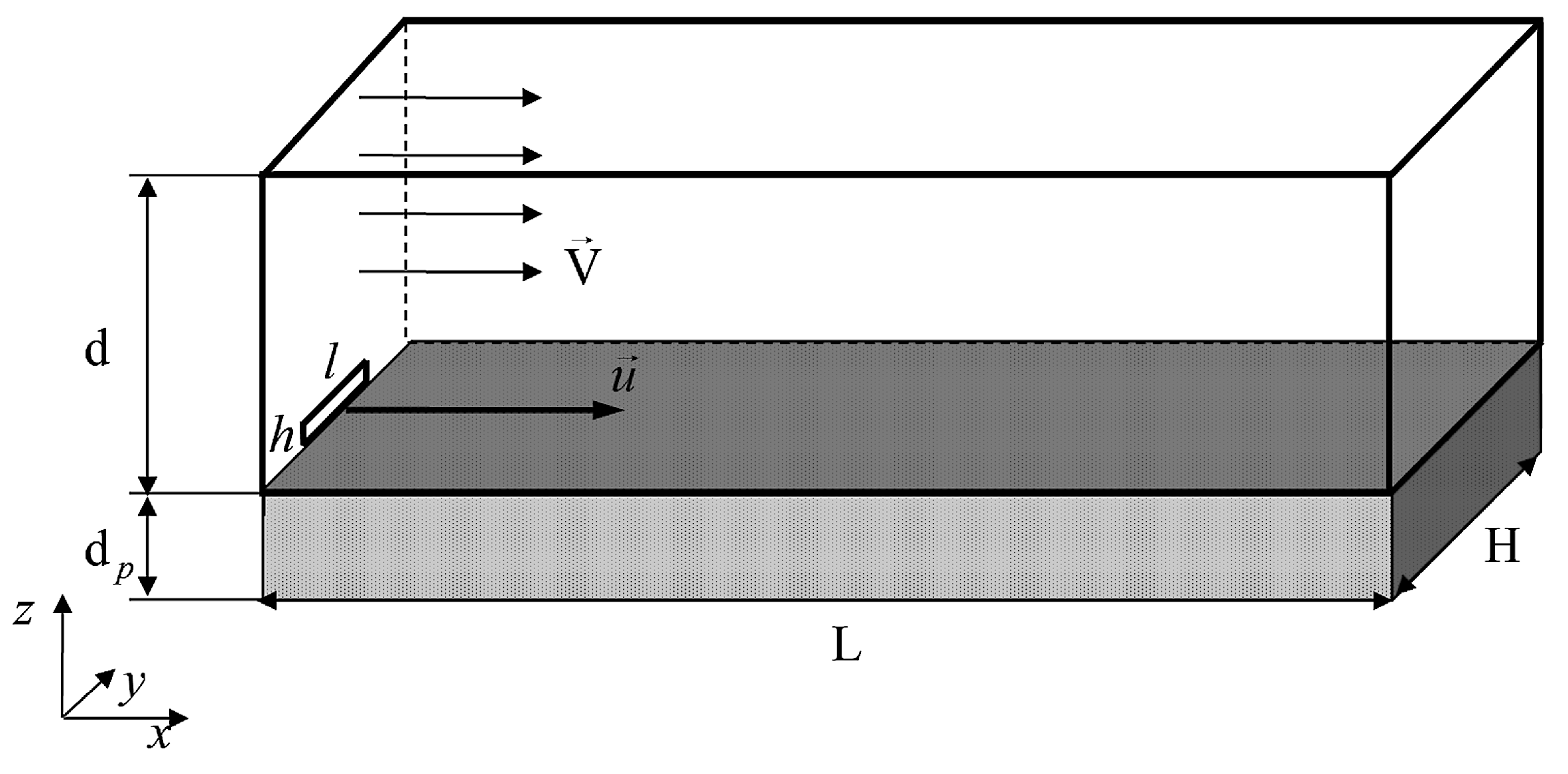
The three-dimensional numerical simulation included two stages. In the first stage, the discharge of waste water from the slot-shaped outlet located at the bottom of the river across its bed was studied. The computational domain shown in Figure 1 represents a rectangular parallelepiped with a single source in the form of a rectangular slot of height $h=0.1$ m and width $l=10$ m, which is centrally located in the vicinity of the bottom at equal distance from the side walls of the domain (the geometry of the discharge source was adopted from [13]). The saline solution with a concentration of $C_0$ flows out from the slot at a constant velocity $\overrightarrow{u}$.

The depth of the reservoir is 10 m, the width of the computational domain is 30 m, and its length L is 200 m. These values correspond to a wide river (such as Kama river), and, at the same time, the domain is large enough to carefully consider a part of the water body that is mostly influenced by the discharge. The brine may substantially affect the hyporheic zone parameters. In particular, the depth of the hyporheic zone can grow because of downstream flows caused by the discharge. Therefore, it is necessary to consider the entire permeable layer in a river bed. We use the usual value of the water-bearing layer depth at a river bottom for the porous layer thickness; thus, ${\mathrm{d}}_p=4$ m.

The bottom soil consists of sand characterized by permeability, $K={10}^{-13}÷{10}^{-15}$ m${}^2$, and porosity, $m=0.5$ (in the presented results $K={10}^{-13}$ if not specified). The inflow velocity of the saline solution corresponds to the minimum flow rate of 0.02 m${}^3/$s used to obtain lower-bound estimates of the accumulative effect of the bottom soil. The velocity of the main flow is $\overrightarrow{V}=0.1$ m/s (which is a 45 typical value for Kama river [70]). The flow is turbulent and characterized by Reynolds numbers on the order of ${10}^6$.

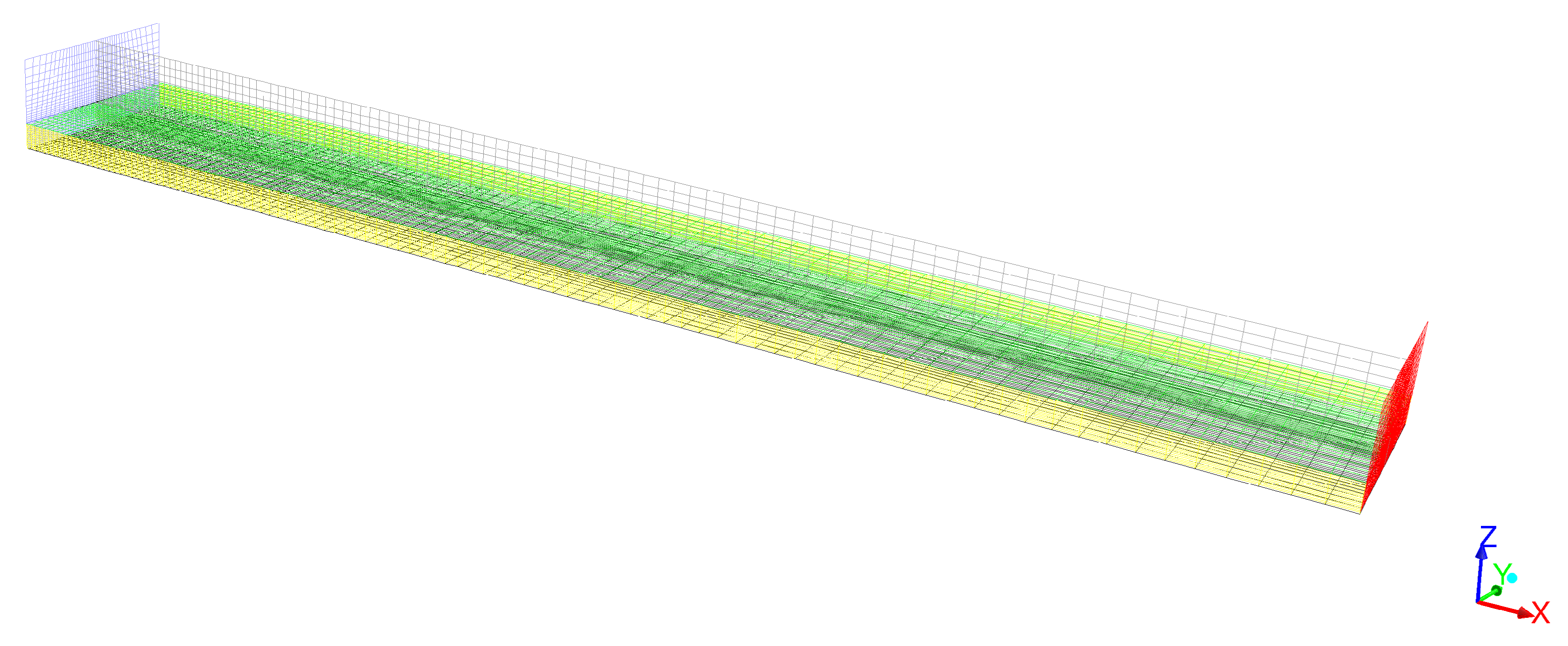
The result of discretizing the computational domain into elements was a mesh with refinement near the outlet (see Figure 2). The small size of the elements at the interface between the surface water and subsurface layers made it possible to consider drastic velocity gradients at the interface. The number of nodes in the longitudinal direction was 256 × 64 and was −45 in the transverse direction. The total number of nodes was 737,280. The minimum spatial step size was 0.001 m, and the maximum size was 1 m. The minimum area of the mesh element was $1.0\times {10}^{-6}$ m${}^2$, and it was located at the interface near the discharge source, while the maximum area of the element was 0.001 m${}^2$, and it was located in the water surface at a considerable distance from the slot. The mesh was created in ANSYS Meshing Software.

2.2. Mathematical Model

Numerical modeling of the propagation of saline waste water in the river was performed within the framework of a three-dimensional approach. The calculations were based on the $k-\epsilon$ model describing turbulent mixing. The problem was solved by applying a nonstationary isothermal approach. The equations of motion in tensor representation for quantities averaged over the Reynolds are as follows [71,72]:

$$\frac{\partial \left(m\rho \right)}{\partial t}+\frac{\partial }{\partial x_i}\left(\rho {\mathrm{v}}_i\right)=0,$$

(1)

$$\begin{array}{c}\hfill \frac{\partial }{\partial t}\left(\frac{1}{m}\rho {\mathrm{v}}_i\right)+\frac{\partial }{\partial x_j}\left(\frac{1}{m^2}\rho {\mathrm{v}}_i{\mathrm{v}}_j\right)=-\frac{\partial p}{\partial x_i}+\frac{\partial }{\partial x_j}\left[\frac{\mu }{m}\left(\frac{\partial {\mathrm{v}}_i}{\partial x_j}+\frac{\partial {\mathrm{v}}_j}{\partial x_i}-\frac{2}{3}{\delta }_{ij}\frac{\partial {\mathrm{v}}_l}{\partial x_l}\right)\right]\\ \hfill +\frac{\partial }{\partial x_j}\left[\frac{{\mu }_t}{m}\left(\frac{\partial {\mathrm{v}}_i}{\partial x_j}+\frac{\partial {\mathrm{v}}_j}{\partial x_i}\right)-\frac{2}{3}\left(\rho k+{\mu }_t\frac{\partial {\mathrm{v}}_l}{\partial x_l}\right){\delta }_{ij}\right]+\frac{\mu }{K}{\mathrm{v}}_i+\rho g_i,\end{array}$$

(2)

where $\rho$ is the density; ${\mathrm{v}}_{\mathrm{i}}$ are the components of the velocity vector (i = 1, 2 and 3, which correspond to the x, y and z axes); $\mu$ is the kinematic viscosity; and m and K are the porosity and permeability of the porous medium, respectively. Turbulent viscosity ${\mu }_t$ is the function of the turbulent kinetic energy k and its dissipation rate $\epsilon$,

$${\mu }_t=\rho C_{\mu }{k}^2/\epsilon ,$$

(3)

where $C_{\mu }$ is a constant.

The equations for the turbulent kinetic energy and its dissipation rate are written as:

$$\frac{\partial }{\partial t}\left(\rho k\right)+\frac{\partial }{\partial x_i}\left(\rho k{\mathrm{v}}_i\right)=\frac{\partial }{\partial x_j}\left[\left(\mu +\frac{{\mu }_t}{{\sigma }_k}\right)\frac{\partial k}{\partial x_j}\right]+G_k+G_b-\rho \epsilon ,$$

(4)

$$\frac{\partial }{\partial t}\left(\rho \epsilon \right)+\frac{\partial }{\partial x_i}\left(\rho \epsilon {\mathrm{v}}_i\right)=\frac{\partial }{\partial x_j}\left[\left(\mu +\frac{{\mu }_t}{{\sigma }_{\epsilon }}\right)\frac{\partial \epsilon }{\partial x_j}\right]+C_{1\epsilon }\frac{\epsilon }{k}{G}_k-C_{2\epsilon }\rho \frac{{\epsilon }^2}{k}.$$

(5)

Here, $G_k={\mu }_t{S}^2$ is the generation of the turbulent kinetic energy due to the average velocity gradient; $g_j$ is the gravitational gravity; ${Pr}_t$ is the turbulent Prandtl number; $C_{1\epsilon },C_{2\epsilon },{\sigma }_k$ and ${\sigma }_{\epsilon }$ are the constants; and $S=\sqrt{2S_{ij}{S}_{ij}}$ is the norm of the tensor of the average strain rate, where

$$S_{ij}=\frac{1}{2}\left(\frac{\partial {\mathrm{v}}_j}{\partial x_i}+\frac{\partial {\mathrm{v}}_i}{\partial x_j}\right).$$

(6)

The equation of the turbulent kinetic energy includes the term

$$G_b=-\frac{g_j({\mu }_t/\rho )}{{Pr}_t}\frac{\partial \rho }{\partial z},$$

(7)

which describes the generation of the turbulent kinetic energy due to buoyancy. In the case of stable stratification $\partial \rho /\partial z<0$ and, due to the fact that the gravity acceleration vector $\overrightarrow{g}$ is directed vertically downward, the above term is negative, which means that the turbulent kinetic energy decreases due to buoyancy. This phenomenon is discussed in detail in [70].

It is assumed that the turbulent transport of matter at a given time and at an arbitrary point of space is determined by the average concentration gradient taken at the same point of space and at the same time (the Boussinesq hypothesis).

$$\frac{\partial }{\partial t}\left(\rho c\right)+\nabla ·\left(\rho \mathbf{v}c\right)=-\nabla ·\mathbf{J}.$$

(8)

Here, $\nabla =\partial /\partial x_j$ is the nabla operator, and $\mathbf{J}$ is the vector of the impurity diffusion flux defined by the expression:

$$\mathbf{J}=-\rho \left(D_m+D_t\right)\nabla c,$$

(9)

where $D_m$ is the coefficient of molecular diffusion, and $D_t$ is the effective coefficient of turbulent diffusion related to the turbulent viscosity ${\mu }_t$ by the expression $D_t=\left({\mu }_t/\phantom{{\mu }_t\rho }\rho \right)/\phantom{\left({\mu }_t/\phantom{{\mu }_t\rho }\rho \right){\mathrm{Sc}}_t}{\mathrm{Sc}}_t$, where ${\mathrm{Sc}}_t$ is the turbulent Schmidt number.

2.3. Boundary Conditions

The boundary conditions for Equations (1)–(9) are given below for different boundaries of the system. In the problem under consideration, the no-slip condition and the zero-mass flux condition were imposed on the rigid boundaries, which were the river bottom and banks:

$${\mathrm{v}}_x={\mathrm{v}}_y={\mathrm{v}}_z=0,\frac{\partial c}{\partial \mathbf{n}}=0,$$

(10)

where n is the vector normal to the boundary.

The velocity of the main flow (the vector of the flow velocity of the surrounding medium was perpendicular to the inlet boundary $\overrightarrow{V}=\left\{V,0,0\right\}$) was set at the inlet of the computational domain; the concentration was assumed to be equal to the background concentration of contaminants in water:

$${\mathrm{v}}_x=V,{\mathrm{v}}_y=0,{\mathrm{v}}_z=0,c=C_0.$$

(11)

The upper boundary of the region, corresponding to the free surface of the fluid, was assumed to be non-deformable and to satisfy the conditions for the absence of the normal velocity component, tangential stresses and impurity flow

$$(\mathbf{v}·\mathbf{n})=0,\frac{\partial {\mathrm{v}}_x}{\partial x_z}+\frac{\partial {\mathrm{v}}_z}{\partial x_x}=0,\frac{\partial {\mathrm{v}}_y}{\partial x_z}+\frac{\partial {\mathrm{v}}_z}{\partial x_y}=0,\frac{\partial c}{\partial \mathbf{n}}=0.$$

(12)

The condition at the outlet of the computational domain was the balance of mass:

$$\underset{S_{in}}{\oint }\rho {\mathrm{v}}_{in}dS-\underset{S_{out}}{\oint }\rho {\mathrm{v}}_{out}dS=0.$$

(13)

The parameters ${\mathrm{Pr}}_t$, $S{c}_t$, $G_{1\epsilon }$, $C_{2\epsilon }$, $C_{\mu }$, ${\sigma }_k$ and ${\sigma }_k$ used in Equations (1)–(9) are the empirical constants, and their values are taken from [71]: ${Pr}_t$ = 0.85, $S{c}_t=0.7$, $C_{1\epsilon }=1.44$, $C_{2\epsilon }=1.92$, $C_{\mu }=0.09$, ${\sigma }_k=1.0$ and ${\sigma }_{\epsilon }=1.3$. The kinematic viscosity was taken to be equal to $\mu =9.34\times {10}^{-7}$ m${}^2$/s, and the molecular diffusion coefficient was $D=1.8\times {10}^{-9}$ m${}^2$/s [73].

Special consideration is given to a quadratic dependence of density on the concentration $\rho ={\rho }_0+Ac+B{c}^2$ (${\rho }_0=999.993$ kg/m${}^3$) with the density difference along the depth being ten percent [70]. The initial data were a zero impurity concentration throughout the water body and the equality of the basic flow velocity to the velocity at the inlet of the computational domain. The finite-volume method was used to perform numerical calculations. The spatial discretization of the problem equations was performed based on the second-order accuracy scheme. The temporal evolution was modeled using an explicit second-order approximation scheme.

2.4. Model Verification

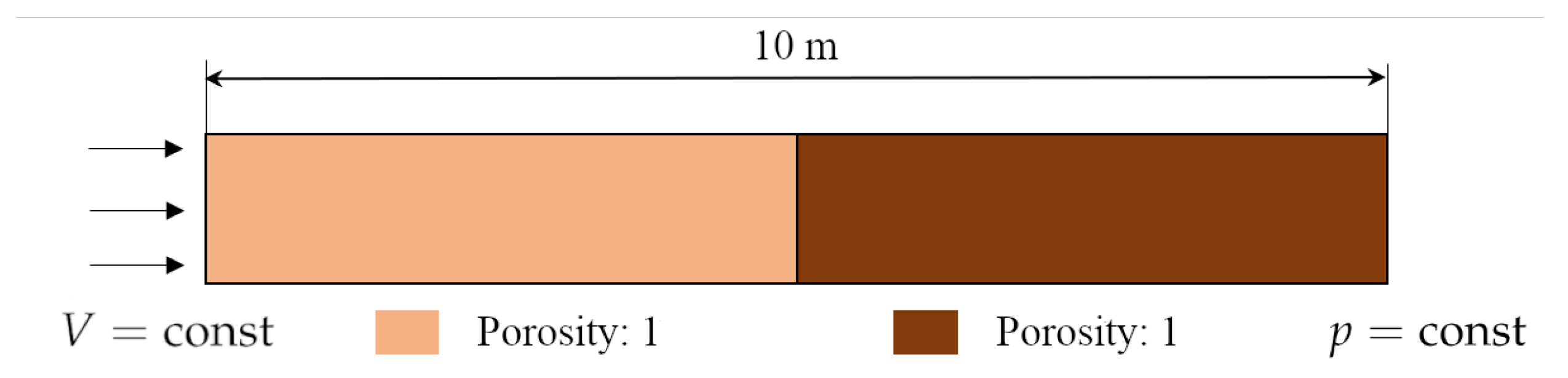
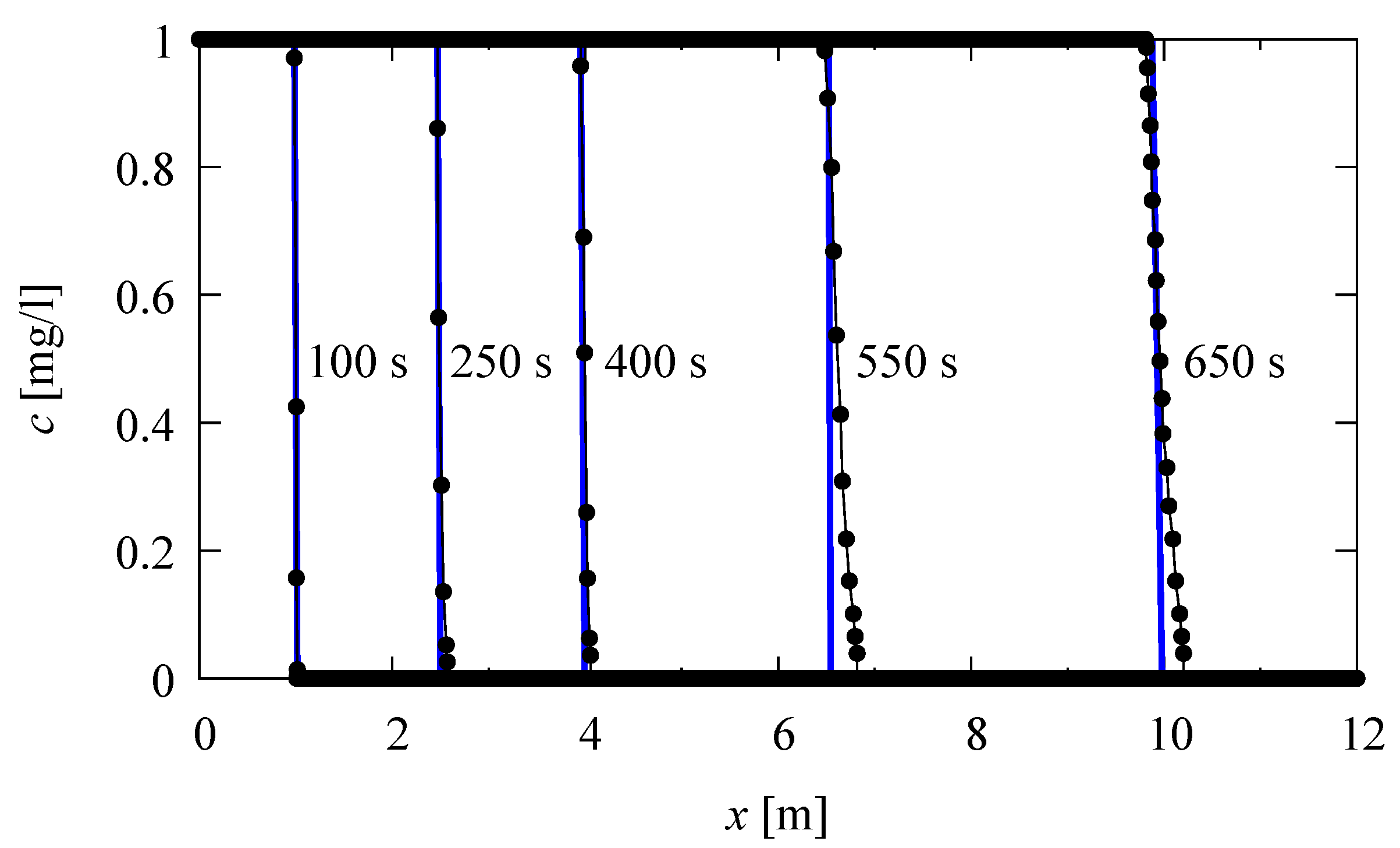
The cases studied by Kinzelbach [74] and Broecker et al. [75] were used to verify the transport application code of the integral equation solver, which was implemented in a domain containing zones of different porosity and permeability. The simulation results were compared with the results of the analytical model applied to the one-dimensional problem of continuous injection considered in [74]. The one-dimensional 10 m long region was divided into two equal parts. One half consisting of water had a porosity of 1, and the other half consisting of soil and water had a porosity of 0.3 that corresponds to an effective grain diameter of 0.01 m (Figure 3). A constant flow with the passive impurity concentration taken as an indicator, with a molecular diffusion coefficient of ${10}^{-9}$ m${}^2$/s, was set at the inlet of the computational area. The inlet flow rate was fixed at the level of 0.01 m/s.

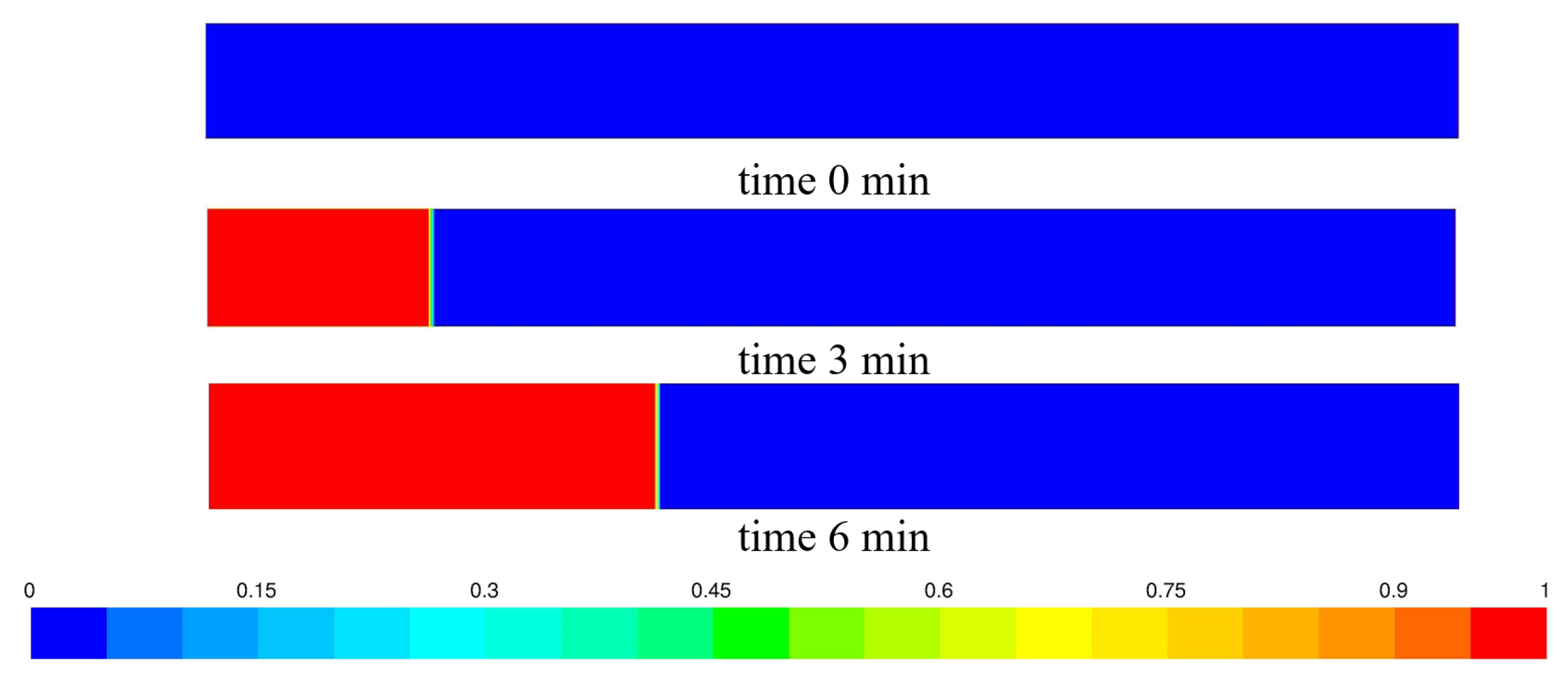
The evolution of the concentration front is shown in Figure 4. At the initial time, the computation area was filled with pure water without impurities. According to the adopted computational scheme, the concentration front propagates through the medium without changing its structure.

The simulated curves of indicator invasion under conditions of constant injection were compared with the analytical results and showed good agreement in the case of transporting conservative indicators through surface water and underground as seen in Figure 5.

3. Results of Numerical Modeling

3.1. Dynamics of the Brine in the River with Sandy Bottom

The numerical simulation of the disposal of excess brines with salt concentration $C_0=300$ g/L [13] was conducted over a period of 24 h. As already mentioned, the brine propagation velocity u was 0.2 m/s, and the velocity of water flow in the river was $V=0.1$ m/s. The average velocity of the fluid motion in the water-saturated layer of the river bottom was ${10}^{-7}$.

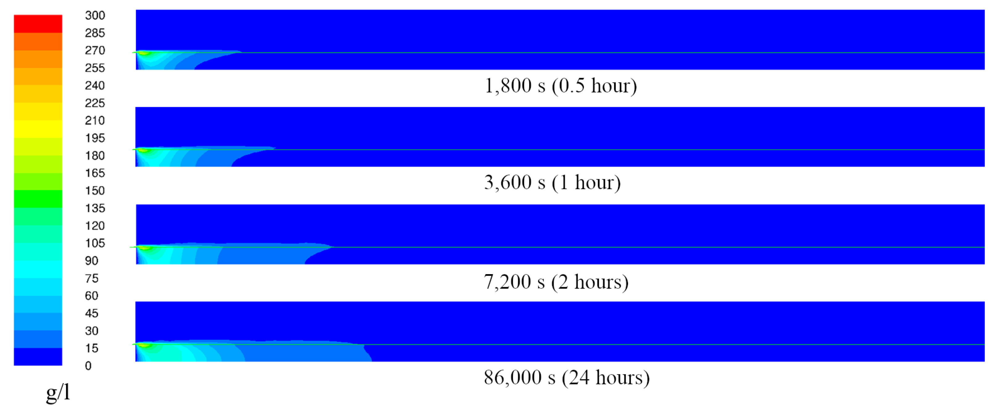
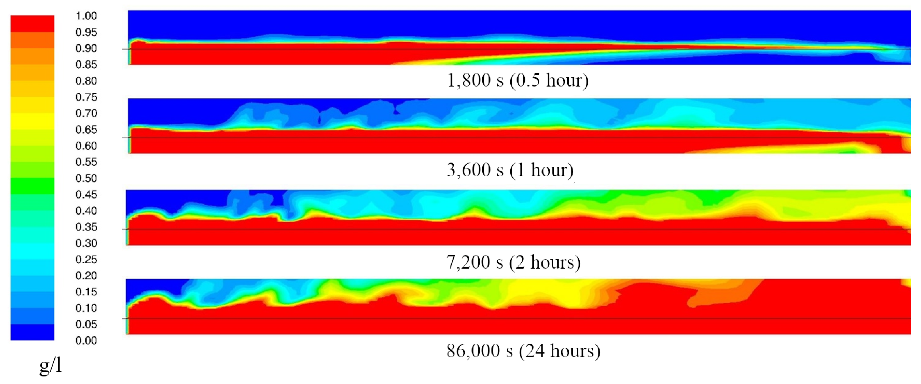
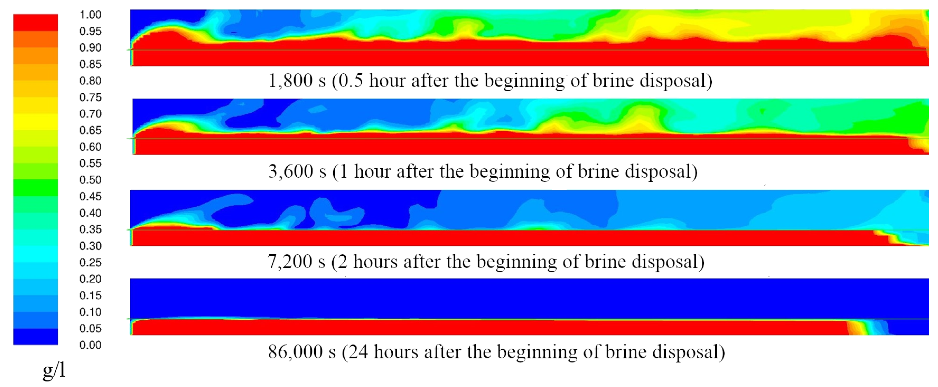
Figure 6 shows the concentration fields for different times after the brine discharge, starting in initially clean water and porous media. The brine spreads with the main stream, and, under the action of gravity, a considerable part moves into the porous medium. In accordance with the regulations, the maximum permissible concentration (MPC) for chlorides in drinking water should not exceed 0.35 g/L and, in fishery waters, 0.3 g/L. The MPC of sulfate in drinking water is 0.5 g/L and is 0.1 g/L in fishery waters. In order to assess compliance with the permitted standards, in Figure 7, the evolution of the salt concentration in the range from 0 to 1 g/L is shown. After 24 h (86,000 s) from the beginning of the brine discharge into the water body, an excess of MPC is observed not only in the bottom layers but also near the river surface.

As can be seen from Figure 6, the depth distribution of impurities is characterized by considerable heterogeneity: heavy impurities are accumulated near the bottom. In the saturated porous medium, the brine spreads vertically downward because the gravity sedimentation of heavy impurity is prevalent in the slow horizontal filtration flow. In the course of time, a non-zero concentration of impurities is observed at a greater distance from the source, and brine accumulation occurs mainly at the porous layer under the river. The estimation of heterogeneity of the concentration distribution throughout the depth of the river shows that, at short distances (a few meters) from the source, the salt concentration at the bottom exceeds its concentration near the surface by hundreds of times.

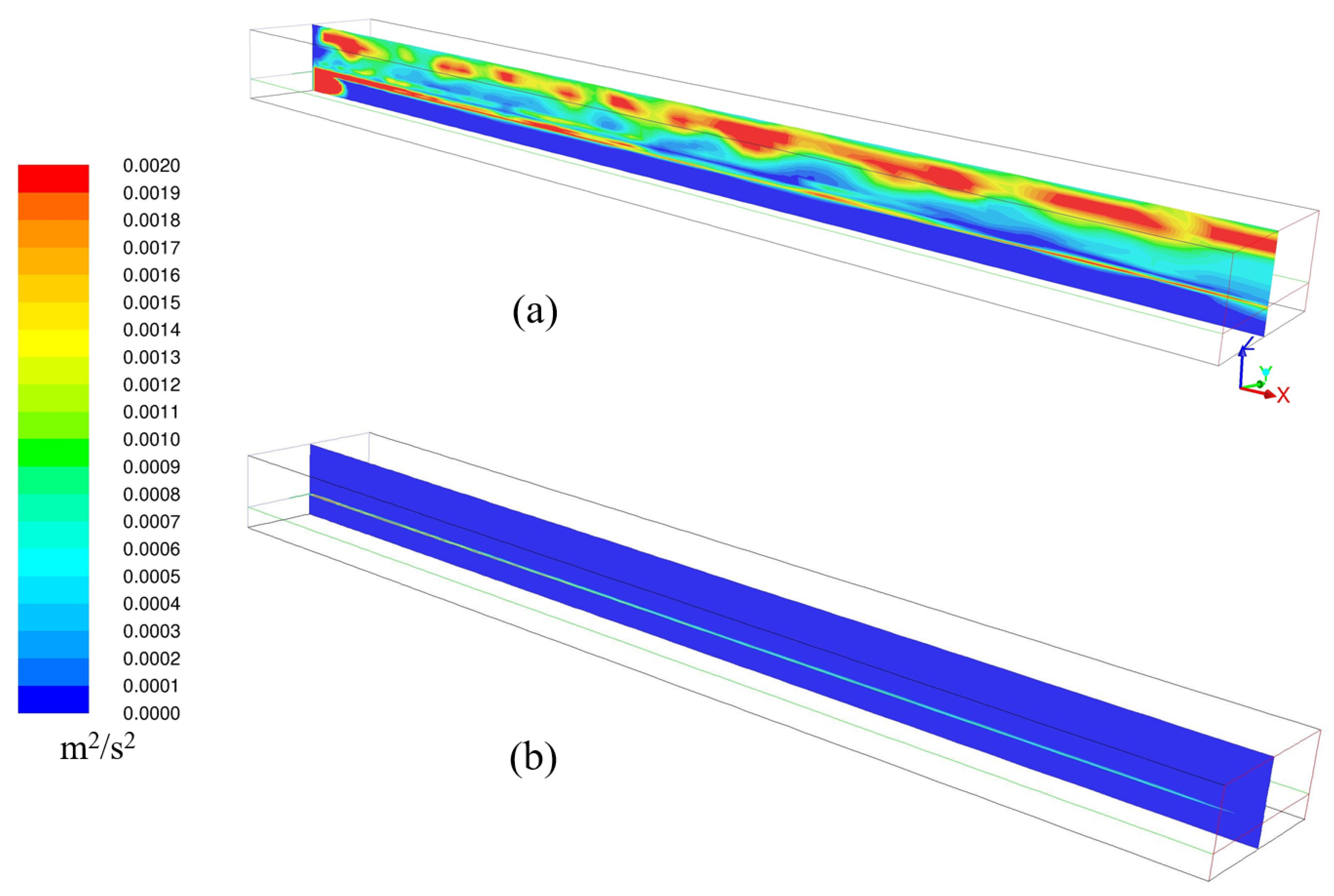
After 12 h, although the dilution process proceeds further, the concentration at the bottom remains practically unchanged. The calculations show that the fluid flow in a free medium become more turbulent in the presence of heavy brines. At an average flow velocity of 0.1 m/s, velocity pulsations reach 3 m/s (see Figure 8 and Figure 9). During brine discharge, the motion near the free surface has the highest kinematic energy (Figure 9a). Vortices of minimum intensity are localized near the bottom; the isosurface of the velocity magnitude of 0.1 m/s is shown in Figure 8a. Such flow patterns determine the transport of brines for long distances from the discharge source, which is similar to a creeping flow. The turbulent diffusion does not lead to complete mixing of impurities with the river water; the propagation of brines through the river bottom occurs without a noticeable decrease in their concentration.

The change in the energy characteristics of the system as a result of disposal of the worked-out brines is demonstrated in Figure 9. Values of the turbulent kinetic energy in a vertical section at the middle of the computational domain are shown for the brine flowing out at a velocity of 0.2 m/s over a period of 24 h and for pure water. The vortex structures generated during propagation of brines grow in size in the horizontal direction with distance from the discharge source (Figure 9a). In the case of pure water outflow, an increase in the turbulent energy is observed only in a thin layer near the porous medium boundary (Figure 9b).

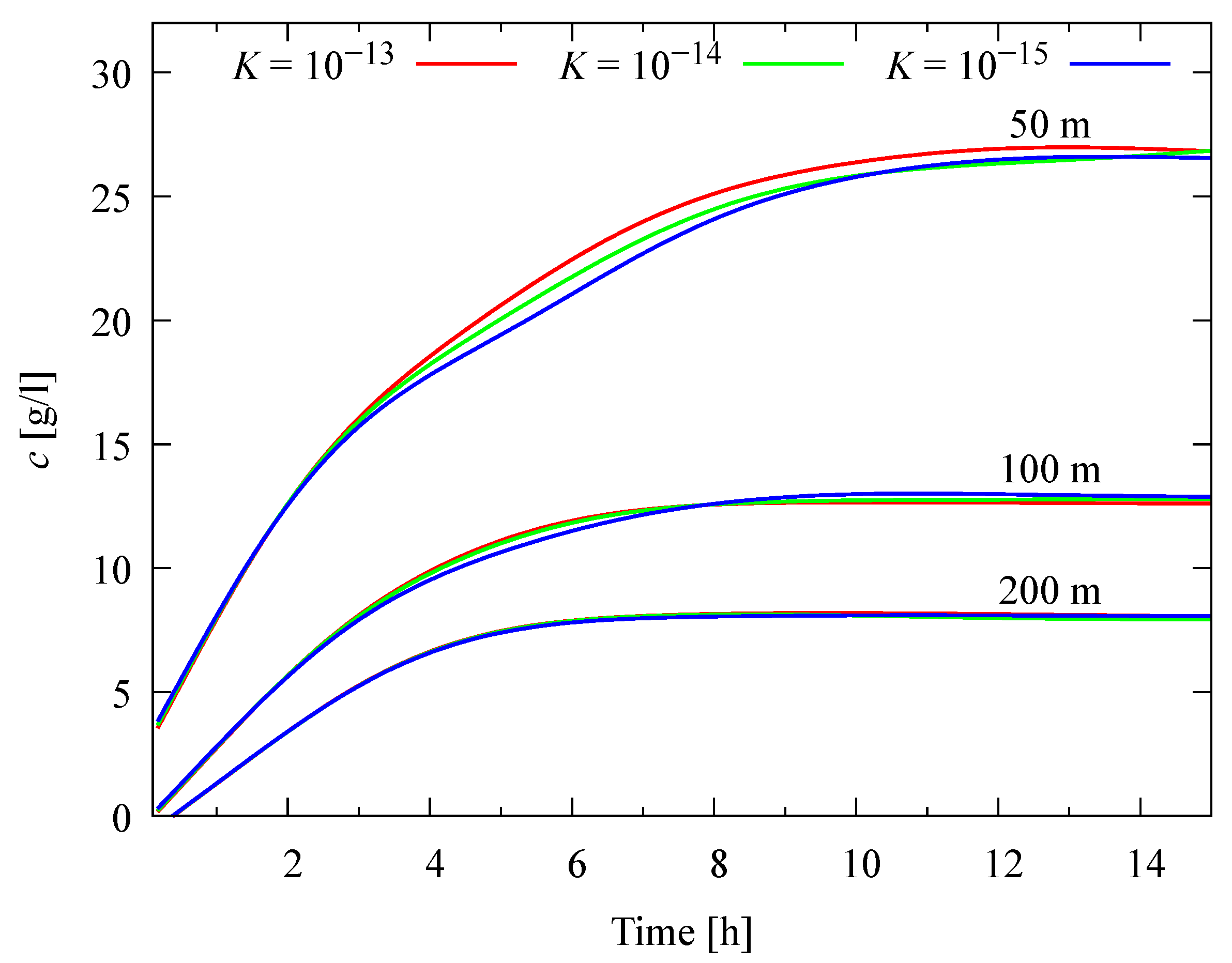
In order to investigate the intensity of the salt accumulation in the soil for different permeabilities, we plotted dependencies of the salt concentration at a depth of 2 m as a function of time (Figure 10). A significant increase in concentration is observed during 12 h near the outlet and during 6 h at a 200 m distance. After those times, saturation is observed, and the concentration almost does not change with time. As one can see, the rate of salt penetration into the soil is weak and depends on the permeability of the porous media for the parameters typical for hyporheic zones. This can be explained by the prevalence of the diffusive mechanism of the porous media saturation at long times.

3.2. Dynamics of Brine Effluent from the Sandy River Bottom

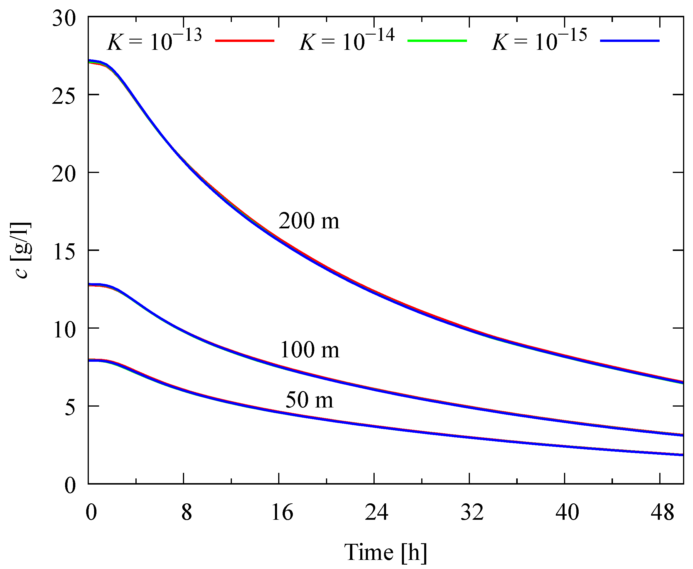
After the brine discharge has been interrupted, the salt concentration in the free liquid layer decreases within a few minutes. An intensive dilution process is observed. At the same time, the salt accumulated in the porous medium layer becomes a new source of contaminant disposal into the water bodies. In the absence of waste water discharge for 24 h, only near half of the salt amount is removed from the soil (see Figure 11 and Figure 12). The remaining amount of salt is washed out gradually, provided the hydrological regime of the water body does not change. As the flow intensity of the river decreases, the rate of impurity removal from the porous medium also decreases. The rate of the salt removal almost does not depend on the permeability coefficient of the porous medium because the process of removal is governed by the diffusion intensity in the hyporheic zone.

The accumulating capacity of the river bottom depends on the composition of the bottom soil. The calculations show that, if the river bottom consists of a sand and gravel mix without a high loam content, the concentration of salts in the bottom soil can exceed the MPC by thousands of times (see Figure 6). The accumulated impurities in the water-bearing layer of the bottom are safe at low- and medium-flow rates. When the river flow increases during the flood period, they can become an intensive source of water body pollution, significantly limiting the water consumption regime for downstream water users.

4. Discussion

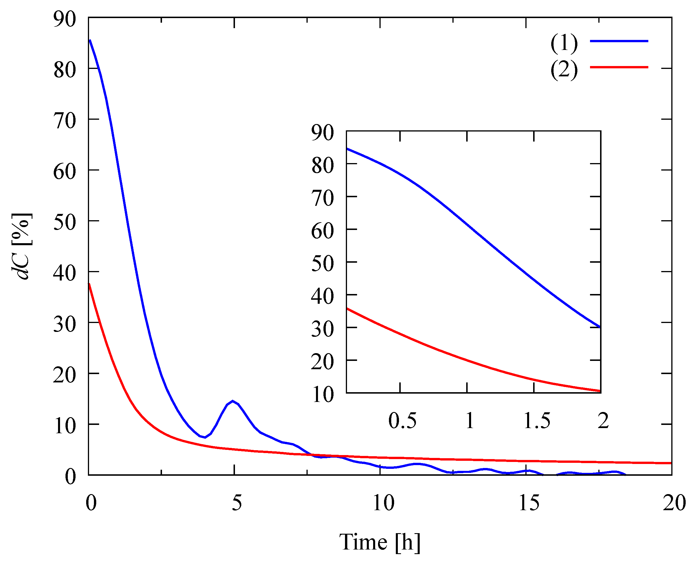
The calculations show that the brine discharge near the river bottom leads to rapid sedimentation of the salt into the porous media layer. In particular, due to a substantial difference between the brine and pure water density, the vertical downwards flow reaches 0.2 mm/s while the value of the average horizontal filtration rate is ${10}^{-4}$ mm/s. Therefore, during the first hour, almost all discharged salt is accumulated by the porous medium. The dependence of the rate of salt absorption by the porous layer in percentage to the discharge rate is shown in Figure 13(1).

After 2 h of waste disposal, the brine reaches the porous medium bottom near the brine outlet, and the process of the accumulation associated with convective motion of the dense brine slows down. At the same time, the impurity continuous to spread in the free water of the river. Therefore, the area affected by the brine rises, which leads to intensification of the diffusion of salt into the porous layer. As a result, after 4 h of discharge, the salt absorption rate of the porous medium begins to grow. After 5 h, the diffusion mechanism of salt transport also slows down. Figure 13 represents the rate of salt washout from the porous layer when the brine discharge is over (see line (2)). A fully saturated hyporheic zone becomes a source of salt pollution, with the output up to 36 percent from the initial brine discharge rate.

It is generally believed that a higher flow rate in a water body leads to more intensive dilution processes, i.e., a lower concentration of contaminants in the water should be observed. However, our calculations show the possibility of the accumulation of a substantial amount of salt in the hyporheic zone. Thus, during high floods due to a soil washout, the efflux of contaminants into the river can have an explosive nature. Therefore, the river bottom near areas of heavy impurity disposal has to be considered as an accumulative source of pollution that creates a threat to safe water use for downstream human settlements.

Conventional approaches in which the maximum concentration of pollutants imposing constraints on the river water consumption is considered only as a consequence of their distribution in a free flow cannot provide a comprehensive explanation of the observed impurity accumulation and distribution effects in water bodies with a hyporheic zone. It is necessary to analyze the accumulative properties of the river bottom, i.e., to solve the problem of free-stream motion over the porous water-bearing layer. Heavy contaminants can result in a sharp increase in the content of contaminants in the river bottom substrate in the vicinity of discharge areas. Such challenging problems often arise at industrial complexes associated with heavy waste waters in the case of the disposal of excess highly mineralized brines into water bodies, where, due to significant year-to-year fluctuations in the water levels and ice regime, the bottom disposal of wastewater is considered to be a preferential option.

5. Conclusions

The numerical simulations performed in this work provided data on the distributions of pollutant concentration through the depth of the water body and in the bottom soil substrate as a result of ’heavy’ wastewater discharge. Significant heterogeneity of the impurity distribution was observed not only near the river bottom but also in the water-saturated layer of the porous medium. In the porous medium near the brine outlet, the impurity propagated vertically downwards at a velocity that was three orders of magnitude higher than the filtration rate in the horizontal direction. With time, a non-zero concentration of impurity was observed at a large distance from the source, and substantial accumulations of salt occurred at the river hyporheic zone.

The evaluation of heterogeneity at the depth of the impurity concentration showed that, at short distances (of the order of a few meters) from the source, the concentration of the impurity at the bottom was thousands of times higher than near the water body surface. The dilution of impurity that occurred thereafter did not dramatically change the concentration at the bottom of the hyporheic zone. The accumulated impurities in the water-bearing layer are safe at low flow rates; however, as the river flow increases during the flood season or, for example, caused by the operating regime of a hydroelectric power plant, they may become an intense source of pollution, which should be considered. Thus, the discharge of waste water with heavy impurities must be organized in such a way so as to ensure that the volume of discharged water waste corresponds to the actual flow rate in the water body and the accumulative capacity of the river bottom.

References

- Salama, R.; Otto, C.; Fitzpatrick, R. Contributions of groundwater conditions to soil and water salinization. Hydrogeol. J. 1999, 7, 46–64. [Google Scholar] [CrossRef]
- Wells, M.G.; Wettlaufer, J.S. The long-term circulation driven by density currents in a two-layer stratified basin. J. Fluid Mech. 2007, 572, 37–58. [Google Scholar] [CrossRef] [Green Version]
- Arle, J.; Wagner, F. Effects of anthropogenic salinisation on the ecological status of macroinvertebrate assemblages in the Werra River (Thuringia, Germany). Hydrobiologia 2012, 701, 129–148. [Google Scholar] [CrossRef]
- Eilers, R.; Eilers, W.; Fitzgerald, M. A Salinity Risk Index for Soils of the Canadian Prairies. HYJO 1997, 5, 68–79. [Google Scholar] [CrossRef]
- Baldwin, D.S.; Rees, G.N.; Mitchell, A.M.; Watson, G.; Williams, J. The short-term effects of salinization on anaerobic nutrient cycling and microbial community structure in sediment from a freshwater wetland. Wetlands 2006, 26, 455–464. [Google Scholar] [CrossRef]
- Lyubimova, T.P.; Lepikhin, A.P.; Parshakova, Y.N.; Tsiberkin, K.B. Numerical modeling of liquid-waste infiltration from storage facilities into surrounding groundwater and surface-water bodies. J. Appl. Mech. Tech. Phy. 2016, 57, 1208–1216. [Google Scholar] [CrossRef]
- Khayrulina, E.; Bogush, A.; Novoselova, L.; Mitrakova, N. Properties of Alluvial Soils of Taiga Forest under Anthropogenic Salinisation. Forests 2021, 12, 321. [Google Scholar] [CrossRef]
- Lyubimova, T.; Lepikhin, A.; Parshakova, Y.; Kolchanov, V.Y.; Gualtieri, C.; Lane, S.; Roux, B. Hydrodynamic Aspects of Confluence of Rivers with Different Water Densities. J. Appl. Mech. Tech. Phys. 2021, 62, 1211–1221. [Google Scholar] [CrossRef]
- Bauer, M.; Eichinger, L.; Elsass, P.; Kloppmann, W.; Wirsing, G. Isotopic and hydrochemical studies of groundwater flow and salinity in the Southern Upper Rhine Graben. Int. J. Earth Sci. (Geol Rundsch) 2005, 94, 565–579. [Google Scholar] [CrossRef]
- Khayrulina, E.; Maksimovich, N. Influence of Drainage with High Levels of Water-Soluble Salts on the Environment in the Verhnekamskoe Potash Deposit, Russia. Mine Water Environ. 2018, 37, 595–603. [Google Scholar] [CrossRef]
- Andreichuk, V.; Eraso, A.; Domínguez, M.C. A large sinkhole in the Verchnekamsky potash basin in the urals. Mine Water Environ. 2000, 19, 2–18. [Google Scholar] [CrossRef]
- Fetisova, N.F.; Fetisov, V.V.; De Maio, M.; Zektser, I.S. Groundwater vulnerability assessment based on calculation of chloride travel time through the unsaturated zone on the area of the Upper Kama potassium salt deposit. Environ. Earth Sci. 2016, 75, 681. [Google Scholar] [CrossRef]
- Lepikhin, A.P.; Lyubimova, T.P.; Parshakova, Y.N.; Tiunov, A.A. Discharge of excess brine into water bodies at potash industry works. J. Min. Sci. 2012, 48, 390–397. [Google Scholar] [CrossRef]
- Lyubimova, T.P.; Lepikhin, A.P.; Parshakova, Y.N. Numerical Simulation of Highly Saline Wastewater Discharge into Water Objects to Improve Discharge Devices. J. Appl. Mech. Tech. Phys. 2020, 61, 1250–1256. [Google Scholar] [CrossRef]
- Jirka, G.H. Integral Model for Turbulent Buoyant Jets in Unbounded Stratified Flows. Part I: Single Round Jet. Environ. Fluid Mech. 2004, 4, 1–56. [Google Scholar] [CrossRef]
- Lai, A.C.H.; Yu, D.; Lee, J.H.W. Mixing of a Rosette Jet Group in a Crossflow. J. Hydraul. Eng. 2011, 137, 787–803. [Google Scholar] [CrossRef]
- Norman, T.L.; Revankar, S.T. Buoyant jet and two-phase jet-plume modeling for application to large water pools. Nucl. Eng. Des. 2011, 241, 1667–1700. [Google Scholar] [CrossRef]
- Lee, J.H.W. Mixing of Multiple Buoyant Jets. J. Hydraul. Eng. 2012, 138, 1008–1021. [Google Scholar] [CrossRef]
- Lai, A.C.H.; Lee, J.H.W. Dynamic interaction of multiple buoyant jets. J. Fluid Mech. 2012, 708, 539–575. [Google Scholar] [CrossRef]
- Lai, C.C.K.; Lee, J.H.W. Initial mixing of inclined dense jet in perpendicular crossflow. Environ. Fluid Mech 2014, 14, 25–49. [Google Scholar] [CrossRef]
- Lyubimova, T.P.; Roux, B.; Luo, S.; Parshakova, Y.N.; Shumilova, N.S. Modeling of the near-field distribution of pollutants coming from a coastal outfall. Nonlinear Process. Geophys. 2013, 20, 257–266. [Google Scholar] [CrossRef] [Green Version]
- Harvey, J.W.; Bencala, K.E. The Effect of streambed topography on surface-subsurface water exchange in mountain catchments. Water Resour. Res. 1993, 29, 89–98. [Google Scholar] [CrossRef]
- Sophocleous, M. Interactions between groundwater and surface water: The state of the science. Hydrogeol. J. 2002, 10, 52–67. [Google Scholar] [CrossRef]
- Boulton, A.J.; Datry, T.; Kasahara, T.; Mutz, M.; Stanford, J.A. Ecology and management of the hyporheic zone: Stream–groundwater interactions of running waters and their floodplains. J. N. Am. Benthol. Soc. 2010, 29, 26–40. [Google Scholar] [CrossRef] [Green Version]
- Hester, E.T.; Gooseff, M.N. Moving Beyond the Banks: Hyporheic Restoration Is Fundamental to Restoring Ecological Services and Functions of Streams. Environ. Sci. Technol. 2010, 44, 1521–1525. [Google Scholar] [CrossRef] [PubMed]
- Krause, S.; Tecklenburg, C.; Munz, M.; Naden, E. Streambed nitrogen cycling beyond the hyporheic zone: Flow controls on horizontal patterns and depth distribution of nitrate and dissolved oxygen in the upwelling groundwater of a lowland river. J. Geophys. Res. Biogeosci. 2013, 118, 54–67. [Google Scholar] [CrossRef]
- Lewandowski, J.; Arnon, S.; Banks, E.; Batelaan, O.; Betterle, A.; Broecker, T.; Coll, C.; Drummond, J.D.; Gaona Garcia, J.; Galloway, J.; et al. Is the Hyporheic Zone Relevant beyond the Scientific Community? Water 2019, 11, 2230. [Google Scholar] [CrossRef] [Green Version]
- Dent, C.L.; Grimm, N.B.; Martí, E.; Edmonds, J.W.; Henry, J.C.; Welter, J.R. Variability in surface-subsurface hydrologic interactions and implications for nutrient retention in an arid-land stream. J. Geophys. Res. Biogeosci. 2007, 112, G04004. [Google Scholar] [CrossRef] [Green Version]
- Buffington, J.M.; Tonina, D. Hyporheic Exchange in Mountain Rivers II: Effects of Channel Morphology on Mechanics, Scales, and Rates of Exchange. Geogr. Compass 2009, 3, 1038–1062. [Google Scholar] [CrossRef]
- Cardenas, M.B. Stream-aquifer interactions and hyporheic exchange in gaining and losing sinuous streams. Water Resour. Res. 2009, 45. [Google Scholar] [CrossRef]
- Ruehl, C.R.; Fisher, A.T.; Los, H.M.; Wankel, S.D.; Wheat, C.G.; Kendall, C.; Hatch, C.E.; Shennan, C. Nitrate dynamics within the Pajaro River, a nutrient-rich, losing stream. J. N. Am. Benthol. Soc. 2007, 26, 191–206. [Google Scholar] [CrossRef]
- Bardini, L.; Boano, F.; Cardenas, M.B.; Revelli, R.; Ridolfi, L. Nutrient cycling in bedform induced hyporheic zones. Geochim. Cosmochim. Acta 2012, 84, 47–61. [Google Scholar] [CrossRef] [Green Version]
- Wu, L.; Singh, T.; Gomez-Velez, J.; Nützmann, G.; Wörman, A.; Krause, S.; Lewandowski, J. Impact of Dynamically Changing Discharge on Hyporheic Exchange Processes Under Gaining and Losing Groundwater Conditions. Water Resour. Res. 2018, 54, 10076–10093. [Google Scholar] [CrossRef]
- Bencala, K.E.; Walters, R.A. Simulation of solute transport in a mountain pool-and-riffle stream: A transient storage model. Water Resour. Res. 1983, 19, 718–724. [Google Scholar] [CrossRef]
- Elliott, A.H.; Brooks, N.H. Transfer of nonsorbing solutes to a streambed with bed forms: Laboratory experiments. Water Resour. Res. 1997, 33, 137–151. [Google Scholar] [CrossRef]
- Packman, A.I.; Salehin, M.; Zaramella, M. Hyporheic Exchange with Gravel Beds: Basic Hydrodynamic Interactions and Bedform-Induced Advective Flows. J. Hydraul. Eng. 2004, 130, 647–656. [Google Scholar] [CrossRef]
- Tonina, D.; Buffington, J.M. Hyporheic exchange in gravel bed rivers with pool-riffle morphology: Laboratory experiments and three-dimensional modeling. Water Resour. Res. 2007, 43, 1–16. [Google Scholar] [CrossRef] [Green Version]
- Dudunake, T.; Tonina, D.; Reeder, W.J.; Monsalve, A. Local and Reach-Scale Hyporheic Flow Response from Boulder-Induced Geomorphic Changes. Water Resour. Res. 2020, 56, e2020WR027719. [Google Scholar] [CrossRef]
- Van der Molen, D.T.; Breeuwsma, A.; Boers, P.C.M. Agricultural Nutrient Losses to Surface Water in the Netherlands: Impact, Strategies, and Perspectives. J. Environ. Qual. 1998, 27, 4–11. [Google Scholar] [CrossRef]
- Lewandowski, J.; Putschew, A.; Schwesig, D.; Neumann, C.; Radke, M. Fate of organic micropollutants in the hyporheic zone of a eutrophic lowland stream: Results of a preliminary field study. Sci. Total Environ. 2011, 409, 1824–1835. [Google Scholar] [CrossRef] [PubMed]
- Engelhardt, I.; Barth, J.A.C.; Bol, R.; Schulz, M.; Ternes, T.A.; Schüth, C.; van Geldern, R. Quantification of long-term wastewater fluxes at the surface water/groundwater-interface: An integrative model perspective using stable isotopes and acesulfame. Sci. Total Environ. 2014, 466–467, 16–25. [Google Scholar] [CrossRef] [PubMed]
- Brunke, M.; Gonser, T. The ecological significance of exchange processes between rivers and groundwater. Freshw. Biol. 1997, 37, 1–33. [Google Scholar] [CrossRef] [Green Version]
- Heberer, T.; Massmann, G.; Fanck, B.; Taute, T.; Dünnbier, U. Behaviour and redox sensitivity of antimicrobial residues during bank filtration. Chemosphere 2008, 73, 451–460. [Google Scholar] [CrossRef]
- Botter, G.; Basu, N.B.; Zanardo, S.; Rao, P.S.C.; Rinaldo, A. Stochastic modeling of nutrient losses in streams: Interactions of climatic, hydrologic, and biogeochemical controls. Water Resour. Res. 2010, 46. [Google Scholar] [CrossRef] [Green Version]
- Huntscha, S.; Singer, H.P.; McArdell, C.S.; Frank, C.E.; Hollender, J. Multiresidue analysis of 88 polar organic micropollutants in ground, surface and wastewater using online mixed-bed multilayer solid-phase extraction coupled to high performance liquid chromatography-tandem mass spectrometry. J. Chromatogr. A 2012, 1268, 74–83. [Google Scholar] [CrossRef] [PubMed]
- Lawrence, J.E.; Skold, M.E.; Hussain, F.A.; Silverman, D.R.; Resh, V.H.; Sedlak, D.L.; Luthy, R.G.; McCray, J.E. Hyporheic Zone in Urban Streams: A Review and Opportunities for Enhancing Water Quality and Improving Aquatic Habitat by Active Management. Environ. Eng. Sci. 2013, 30, 480–501. [Google Scholar] [CrossRef]
- Regnery, J.; Barringer, J.; Wing, A.D.; Hoppe-Jones, C.; Teerlink, J.; Drewes, J.E. Start-up performance of a full-scale riverbank filtration site regarding removal of DOC, nutrients, and trace organic chemicals. Chemosphere 2015, 127, 136–142. [Google Scholar] [CrossRef] [PubMed]
- Schaper, J.L.; Posselt, M.; Bouchez, C.; Jaeger, A.; Nuetzmann, G.; Putschew, A.; Singer, G.; Lewandowski, J. Fate of Trace Organic Compounds in the Hyporheic Zone: Influence of Retardation, the Benthic Biolayer, and Organic Carbon. Environ. Sci. Technol. 2019, 53, 4224–4234. [Google Scholar] [CrossRef]
- Schaper, J.L.; Posselt, M.; McCallum, J.L.; Banks, E.W.; Hoehne, A.; Meinikmann, K.; Shanafield, M.A.; Batelaan, O.; Lewandowski, J. Hyporheic Exchange Controls Fate of Trace Organic Compounds in an Urban Stream. Environ. Sci. Technol. 2018, 52, 12285–12294. [Google Scholar] [CrossRef] [PubMed] [Green Version]
- Zarnetske, J.P.; Haggerty, R.; Wondzell, S.M.; Baker, M.A. Dynamics of nitrate production and removal as a function of residence time in the hyporheic zone. J. Geophys. Res. Biogeosci. 2011, 116, G01025. [Google Scholar] [CrossRef]
- Gomez, J.D.; Wilson, J.L.; Cardenas, M.B. Residence time distributions in sinuosity-driven hyporheic zones and their biogeochemical effects. Water Resour. Res. 2012, 48, W09533. [Google Scholar] [CrossRef]
- Marzadri, A.; Tonina, D.; Bellin, A. Morphodynamic controls on redox conditions and on nitrogen dynamics within the hyporheic zone: Application to gravel bed rivers with alternate-bar morphology. J. Geophys. Res. Biogeosci. 2012, 117, G00N10. [Google Scholar] [CrossRef] [Green Version]
- Arnon, S.; Yanuka, K.; Nejidat, A. Impact of overlying water velocity on ammonium uptake by benthic biofilms. Hydrol. Process. 2013, 27, 570–578. [Google Scholar] [CrossRef]
- Trauth, N.; Schmidt, C.; Vieweg, M.; Oswald, S.E.; Fleckenstein, J.H. Hydraulic controls of in-stream gravel bar hyporheic exchange and reactions. Water Resour. Res. 2015, 51, 2243–2263. [Google Scholar] [CrossRef]
- Kasahara, T.; Wondzell, S.M. Geomorphic controls on hyporheic exchange flow in mountain streams. Water Resour. Res. 2003, 39, 1005. [Google Scholar] [CrossRef] [Green Version]
- Peterson, E.W.; Sickbert, T.B. Stream water bypass through a meander neck, laterally extending the hyporheic zone. Hydrogeol. J. 2006, 14, 1443–1451. [Google Scholar] [CrossRef]
- Gariglio, F.P.; Tonina, D.; Luce, C.H. Spatiotemporal variability of hyporheic exchange through a pool-riffle-pool sequence. Water Resour. Res. 2013, 49, 7185–7204. [Google Scholar] [CrossRef]
- Fox, A.; Boano, F.; Arnon, S. Impact of losing and gaining streamflow conditions on hyporheic exchange fluxes induced by dune-shaped bed forms. Water Resour. Res. 2014, 50, 1895–1907. [Google Scholar] [CrossRef]
- Cardenas, M.B.; Wilson, J.L. Dunes, turbulent eddies, and interfacial exchange with permeable sediments. Water Resour. Res. 2007, 43, 1–16. [Google Scholar] [CrossRef]
- Cardenas, M.B.; Wilson, J.L. Exchange across a sediment–water interface with ambient groundwater discharge. J. Hydrol. 2007, 346, 69–80. [Google Scholar] [CrossRef]
- Jin, G.; Tang, H.; Li, L.; Barry, D.A. Hyporheic flow under periodic bed forms influenced by low-density gradients. Geophys. Res. Lett. 2011, 38, 1–6. [Google Scholar] [CrossRef] [Green Version]
- Trauth, N.; Schmidt, C.; Maier, U.; Vieweg, M.; Fleckenstein, J.H. Coupled 3-D stream flow and hyporheic flow model under varying stream and ambient groundwater flow conditions in a pool-riffle system. Water Resour. Res. 2013, 49, 5834–5850. [Google Scholar] [CrossRef]
- Trauth, N.; Schmidt, C.; Vieweg, M.; Maier, U.; Fleckenstein, J.H. Hyporheic transport and biogeochemical reactions in pool-riffle systems under varying ambient groundwater flow conditions. J. Geophys. Res. Biogeosci. 2014, 119, 910–928. [Google Scholar] [CrossRef]
- Nützmann, G.; Mey, S. Model-based estimation of runoff changes in a small lowland watershed of north-eastern Germany. J. Hydrol. 2007, 334, 467–476. [Google Scholar] [CrossRef]
- VanderKwaak, J.E. Numerical Simulation of Flow and Chemical Transport in Integrated Surface-Subsurface Hydrologic Systems. Ph.D. Thesis, University of Waterloo, Waterloo, ON, Canada, 1999. [Google Scholar]
- Brunner, P.; Cook, P.G.; Simmons, C.T. Hydrogeologic controls on disconnection between surface water and groundwater. Water Resour. Res. 2009, 45, 1–13. [Google Scholar] [CrossRef] [Green Version]
- Brunner, P.; Simmons, C.T. HydroGeoSphere: A Fully Integrated, Physically Based Hydrological Model. Groundwater 2012, 50, 170–176. [Google Scholar] [CrossRef] [Green Version]
- Alaghmand, S.; Beecham, S.; Jolly, I.D.; Holland, K.L.; Woods, J.A.; Hassanli, A. Modelling the impacts of river stage manipulation on a complex river-floodplain system in a semi-arid region. Environ. Model. Softw. 2014, 59, 109–126. [Google Scholar] [CrossRef]
- Li, B.; Liu, X.; Kaufman, M.H.; Turetcaia, A.; Chen, X.; Cardenas, M.B. Flexible and Modular Simultaneous Modeling of Flow and Reactive Transport in Rivers and Hyporheic Zones. Water Resour. Res. 2020, 56, e2019WR026528. [Google Scholar] [CrossRef]
- Lyubimova, T.; Lepikhin, A.; Konovalov, V.; Parshakova, Y.; Tiunov, A. Formation of the density currents in the zone of confluence of two rivers. J. Hydrol. 2014, 508, 328–342. [Google Scholar] [CrossRef]
- Launder, B.E.; Spalding, D.B. Lectures in Mathematical Models of Turbulence; Academic Press: London, UK; New York, NY, USA, 1972. [Google Scholar]
- Isaevich, A.; Semin, M.; Levin, L.; Ivantsov, A.; Lyubimova, T. Study on the Dust Content in Dead-End Drifts in the Potash Mines for Various Ventilation Modes. Sustainability 2022, 14, 3030. [Google Scholar] [CrossRef]
- Lobo, V.M.; Ribeiro, A.C.; Verissimo, L.M. Diffusion coefficients in aqueous solutions of potassium chloride at high and low concentrations. J. Mol. Liq. 1998, 78, 139–149. [Google Scholar] [CrossRef] [Green Version]
- Kinzelbach, W. Numerische Methoden zur Modellierung des Transports von Schadstoffen im Grundwasser; Oldenbourg: Oldenbourg, Germany, 1992. [Google Scholar]
- Broecker, T.; Sobhi Gollo, V.; Fox, A.; Lewandowski, J.; Nützmann, G.; Arnon, S.; Hinkelmann, R. High-Resolution Integrated Transport Model for Studying Surface Water–Groundwater Interaction. Groundwater 2021, 59, 488–502. [Google Scholar] [CrossRef] [PubMed]
Figure 1.
Geometry of the computational domain containing a culvert pipe in the form of a slot located near the bottom.
Figure 2.
Geometry of the computational domain, including the culvert pipe opening in the form of a slot located near the bottom on the left. The gray color shows the plane section of the computational domain (plane m). The green color indicates the boundary between the composite and porous media. The outlet of the computational domain is shown in red. The location of the porous medium is shown in yellow.
Figure 3.
Schematic representation of the problem of continuous injection in the area containing zones with different porosities and permeabilities.
Figure 4.
Temporal evolution of the concentration front in the continuous injection problem.
Figure 5.
Comparison between simulated (points) and analytically calculated concentrations (lines) found in [74] under conditions of constant injection.
Figure 6.
The impurity concentration fields in a vertical section in the middle of the computation domain. The concentration scale is from 0 to 300 g/L.
Figure 7.
The impurity concentration field in a vertical section at the middle of the calculation domain. The concentration scale is from 0 to 1 g/L.
Figure 8.
The impurity concentration field shown on an isosurface of velocity magnitudes of (a) 0.1 m/s and (b) 0.2 m/s after 24 h of the discharge starting.
Figure 9.
The field of kinetic turbulent energy in a vertical section at the middle of the computational domain: (a) for brine flow at a velocity of 0.2 m/s from a linear source of height 0.1 m and length 10 m over a period of 24 h and (b) for the same source of pure water.
Figure 10.
Evolution of the salt concentration at 2 m deep inside the hyporheic zone of 4 m total depth at distances of 50, 100 and 200 m from the brine source for different permeabilities of the porous medium.
Figure 11.
Variation of soil impurity concentration with time at a depth of 2 m at distances of 50, 100 and 200 m for different permeabilities after the cessation of brine disposal.
Figure 12.
The impurity concentration in a vertical section at the middle of the computational domain after the cessation of brine disposal.
Figure 13.
The dimensionless rate of salt absorption by the porous layer (1) and the dimensionless rate of salt desorption from the saturated state after stopping the brine discharge (2).
Publisher’s Note: MDPI stays neutral with regard to jurisdictional claims in published maps and institutional affiliations. |
© 2022 by the authors. Licensee MDPI, Basel, Switzerland. This article is an open access article distributed under the terms and conditions of the Creative Commons Attribution (CC BY) license (https://creativecommons.org/licenses/by/4.0/).
Share and Cite
MDPI and ACS Style
Parshakova, Y.; Ivantsov, A. Dynamics of Pollution in the Hyporheic Zone during Industrial Processing Brine Discharge. Water 2022, 14, 4006. https://doi.org/10.3390/w14244006
AMA Style
Parshakova Y, Ivantsov A. Dynamics of Pollution in the Hyporheic Zone during Industrial Processing Brine Discharge. Water. 2022; 14(24):4006. https://doi.org/10.3390/w14244006
Chicago/Turabian StyleParshakova, Yanina, and Andrey Ivantsov. 2022. "Dynamics of Pollution in the Hyporheic Zone during Industrial Processing Brine Discharge" Water 14, no. 24: 4006. https://doi.org/10.3390/w14244006
Note that from the first issue of 2016, this journal uses article numbers instead of page numbers. See further details here.