Exploring the Influences of Stream Network Structure and Connectivity on Water Environment Risk in China

Abstract

Stream networks are the transportation channels of pollutants that can significantly influence water environment risk (WER). However, the influences of stream network structure and connectivity (SC) on WER at the national scale and its regional variability have been rarely investigated in China. In this study, the WER was assessed from the grey water footprint of nitrogen and phosphorus in 214 catchments in China. The relationship between WER and SC and its regional variability were analyzed using correlation and grey relational analysis. Results showed that the water environment risk index (RI) in some catchments located in the Hai and Liao River Basins was the highest in China (RI > 0.8). On national scale, longitudinal connectivity (C_l) and cyclical connectivity (C_c) had the strongest influences on WER with grey relational degree index (GRAI) of 0.68 and 0.67, respectively. The average slope (S_r) was the most important in humid zones, whereas C_l and water surface ratio (R_w) had a stronger influence in arid zones. In zones with intensive human activities, C_c, river density (R_d), and the node connection ratio (R_nc) mostly affected WER. The main influenced factors varied significantly among nationwide and different zones, which indicated that climate and human activities played an important role in the spatial variation of the relationship between WER and SC. This study highlights the important role of SC on WER and that the relationship between WER and SC varies with climate and human activities.

1. Introduction

With the acceleration of urbanization and rapid industrial and agricultural development, a large number of pollutants are discharged into river channels and water bodies [1,2,3,4], which increases the water environment risk (WER). Similar to most developing countries, water pollution (e.g., surface water eutrophication and water quality decline) is one of the most critical environmental problems in China with rapid urbanization and economic development [5,6]. Over the past few decades, sewage discharge in China has shown an increasing trend [7], and water quality in 20.6% of surface water falls into class V or worse according to statistics [8]. Rivers, lakes, and other water bodies form a complex and interconnected stream network in China, which is related to the WER due to the water cycle, pollutant transport, and biogeochemical processes [9,10]. Generally, point source pollution directly discharged into rivers and non-point source pollution driven by rainfall-runoff and discharged into stream networks are mainly collected and transported by rivers, and the transfer and dilution of pollutants are affected by the stream network structure and connectivity (SC) [11,12]. Several studies confirmed the impact of SC on WER in some catchments [10,11,13]. However, the spatial variations in WER and its response to SC at the national scale in China have rarely been investigated.

Numerous studies showed that the number, morphology, and connectivity characteristics of stream networks and topography significantly impact the catchment water quality [10,11,14]. For example, Yu et al., revealed that the water surface ratio played a key role in affecting water quality in the Yangtze River Delta plain [10]. Zhao et al., indicated that river density had a positive correlation with water quality in Shanghai [15]. Helton et al. found that the shape of the stream network could affect the removal of NO₃⁻ [16]. Lyu et al., stated that the concentration and distribution of phosphorus were affected by river connectivity in Jiangsu Province [9], and a case in America reported that water quality parameters of most dry seasons were related to topographic features such as slope [17]. Janardan pointed out the influences of mean slope and water surface ratio on total phosphorus at different scales in the Han River basin, South Korea [18], Carlson Mazur stated the impact of hydrologic connectivity on water quality in the Wabash-White watershed [19]. However, in earlier studies, the main driving stream network structure and connectivity characteristics (SCCs) that affected water quality were unclear and dissimilar in different catchments. For example, river length was the key factor affecting total organic carbon (TOC) in the Nakdong River basin [20]; Knoll et al., found that elevated trophic status in Ohio lakes in the US were associated with shallow lake depth and high catchment-to-water surface area ratio [21]. In China, Dou et al., found that the node connection rate and river density had the greatest impact on the water quality of Zhengzhou City [13]; the water surface ratio was the main factor affecting water quality in the Southern Jiangsu Plain and Yangtze River delta plain while the influence of the node connection ratio in these two areas was relatively weak [10,11,14]. Thus, identifying the main driving SCCs at the national scale while elucidating regional differences in the main driving SCCs can provide a sound understanding of the relationship between WER and SC. However, such investigations have rarely been conducted at the national scale.

In addition to SC, climate, human activities, land-use types, and topography are also important driving factors affecting water quality [22,23,24,25,26]. Jiang et al., investigated the relationship between climate and river water quality on a global scale, using the elasticity approach [27]. Kaushal et al., summarized the origins, evolution, and resilience of diverse water quality responses to extreme climate events [28]. Liu et al., reported that human activities significantly affected the water quality of the Hongze Lake [23]. Nguyen stated the pollution source of human activities (industrial, agricultural, and residential sources) directly affected surface water quality in southwestern Vietnam [29]. Yu et al., and You et al., found that land-use type and topography also strongly influenced water quality [26,30]. Meanwhile, SCCs are also affected by climate and human activity [31,32,33,34]. Kreiling found that both water body area and number were affected by climate change and anthropogenic water exploitation in the Fox River watershed [35]. Ranjbar et al., revealed the systematic impacts of climate forcing on the stream network topology and geometry in basins with drainage density in America [36]. Luo et al., quantified the relationship between the human activity intensity and evolution of the SC in the Shaying River basin [31]. Therefore, climate and human activities may also have confounding effects on the correlation between WER and SC. These confounding influences may not be important at small spatial scales or for specific cases but should be considered at large spatial scales with significant spatial differences in climate and human activities.

Therefore, the overall objective of this study is to explore the spatial variability of the relationship between WER and SC under the impact of climate and human activities. This study analyzed the relationship between WER and SC at a large spatial scale and its spatial difference was revealed by grouping level-Ⅲ catchments according to climate and human activity intensity. In this study, the WER was estimated using the water pollution levels of nitrogen and phosphorus at the catchment scale, and the relationship between WER and SC was investigated using the correlation analysis method and grey relational analysis at the national and regional scales. The specific objectives of this study were to: (1) estimate the WER and calculate SCCs in China at the level-Ⅲ catchment scale; (2) explore the relationship between WER and SC at a national scale; and (3) explore the regional variabilities in the relationship between WER and SC by further considering the impact of climate and human activities.

2. Materials and Methods

2.1. Study Area

China is a vast country with wide latitude and different mountain orientations, and has a varied topography including mountainous regions, plateaus, basins, plains, and hills. China has a complex climate with monsoon, temperate continental, and alpine climates in the east, northwest, and on the Qinghai-Tibet Plateau, respectively. The total volume of water resources, including many rivers and lakes, is abundant in China, which include more than 1500 rivers with a drainage area above 1000 km², more than 2800 natural lakes with an area above 1 km², and a large number of dams and hydropower stations, forming a complex stream network. China is divided and sub-divided into successively smaller water resource regions which are classified into three levels: level-I (Figure 1b), level-II, and level-Ⅲ (Figure 1a) catchments. The 10 level-I catchments are divided according to the integrity of major river basins in China, and the 80 level-Ⅱ and 214 level-Ⅲ catchments are divided according to the distribution of tributary river systems and the opinions of local management departments [37]. The area of the level-Ⅲ catchments was ranging from 2.98 × 10³ to 7.03 × 10⁵ km², and mainly concentrated at 2.00 × 10⁴~5.00 × 10⁴ km². The values of WER and SCCs were calculated at the level-Ⅲ catchment scale in this study.

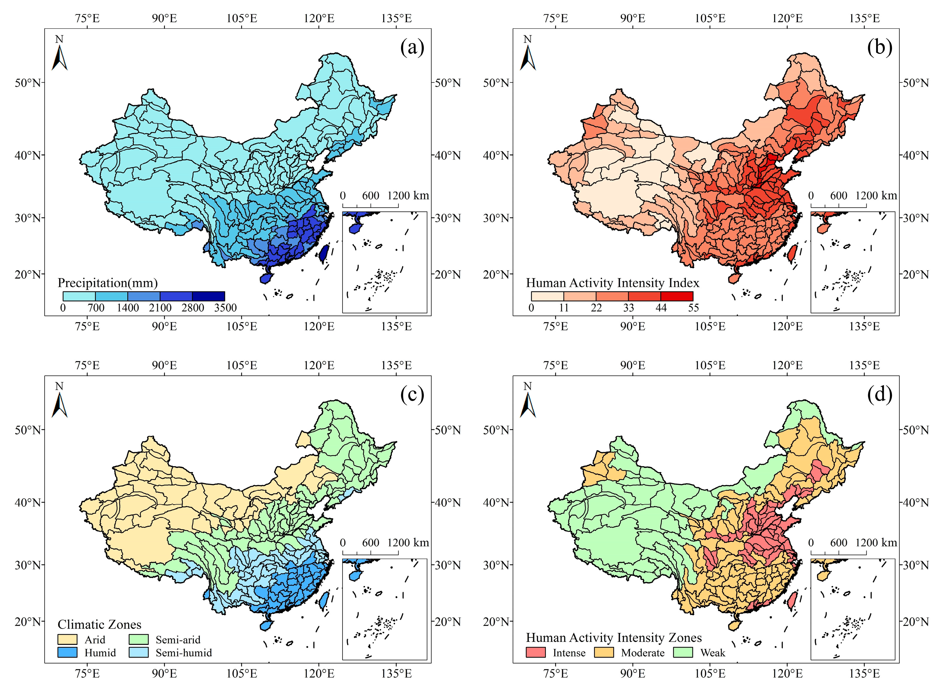
Precipitation and human activity intensity have strong spatial variability in China (Figure 2). The mean annual precipitation of each catchment was calculated by the area-weighted average method using the China Meteorological Forcing Dataset (CMFD) with a spatial resolution of 0.1° × 0.1° [38]. The mean annual precipitation in level-Ⅲ catchments ranged from 75 to 3340 mm and decreased from the southeast to the northwest. The human activity intensity index data were comprehensively calculated from several aspects of human influence, including population density, land transformation, accessibility, and electrical power infrastructure, at a spatial resolution of 1 km × 1 km. The human activity intensity index data were jointly produced by the Center for International Earth Science Information Network (CIESIN) at Columbia University and the Wildlife Conservation Society [39], and was area-weighted and averaged to the level-Ⅲ catchment scale. It ranged from 2.8 to 50.6. Human activities in North China were the most intense, while the Qinghai-Tibet Plateau and Northwest China were less affected by human activities.

2.2. Proposed Water Environment Risk Index (RI)

In this study, WER was assessed based on the water pollution level (WPL). The WPL is the ratio of grey water footprint (GWF) of pollutants to local river runoff and was widely used to assess regional water pollution status [40,41,42]. GWF was developed to evaluate WPL and was applied in many fields [43], such as agricultural, industrial, domestic, and GWF flows between regions [44]. WPL of nitrogen (N_wpl) and phosphorus (P_wpl) were selected to assess catchment water pollution degree (WP), as nitrogen and phosphorus are the two main pollutants affecting water quality [45,46,47] and high-resolution pollutant records of nitrogen and phosphorus are available nationwide. The WP was reflected by the maximum values of N_wpl and P_wpl and was calculated as follows:

$${WP=\max (N}_{wpl}{, P}_{wpl})$$

(1)

$$N_{wpl}=\raisebox{1ex}{$N_{gwf}$}\!\left/ \!\raisebox{-1ex}{$\overline{R}$}\right.$$

(2)

$$P_{wpl}=\raisebox{1ex}{$P_{gwf}$}\!\left/ \!\raisebox{-1ex}{$\overline{R}$}\right.$$

(3)

where N_gwf and P_gwf are the catchment grey water footprints of nitrogen and phosphorus with units of mm/yr, respectively, and $\overline{R}$ is the annual mean runoff with units of mm/yr. N_gwf and P_gwf were obtained from Mekonnen and Hoekstra [41] and Mekonnen and Hoekstra [42], respectively, which were estimated at a spatial resolution of 0.083° × 0.083° for the period 2002–2010 using multi-source data (e.g., crop distributions from Chad et al. [48], and the rate of mineral fertilizer applied to major crops from IFA, et al.). $\overline{R}$ is the gridded runoff at a spatial resolution of 0.5° × 0.5° for the period 2002–2010, and an optimal weighting approach was applied to merge runoff estimated from eight hydrological models constrained by observational streamflow records [49]. Datasets with different spatial resolutions were rasterized to 0.5° × 0.5° resolution using ArcGIS 10.7 software to calculate the grid WP, and then the area-weighted average method was used to calculate the catchment scale WP.

The extreme value standardization method was used to scale WP to 0–1.0. The standardized WP was used as the proposed RI, and was calculated as follows:

$$R I=\frac{{WP-WP}_{min,95}}{{WP}_{max,95}{-WP}_{min,95}}$$

(4)

where WP_min,95 and WP_max,95 are the minimum and maximum 95% fractals of all catchment WP, respectively. Equation (4) considers the possible influence of outliers caused by the data uncertainty. This method can prevent one or a few outliers from having a dramatic impact on the scaling of all other data [50,51].

2.3. Stream Network Structure and Connectivity Characteristics (SCCs)

Based on earlier studies, six SCCs, namely river density (R_d), water surface ratio (R_w), average slope (S_r), longitudinal connectivity (C_l), cyclical connectivity (C_c), and node connection ratio (R_nc), were selected to explore their potential effects on WER. Details of the calculation equations, implications for water quality, and references of these six SCCs are shown in

Table 1. Stream network structure and connectivity characteristics (SCCs).

Indexes	Formula	Implication for Water Quality	Reference
River density	$R_d=\frac{L}{A}$	Level of pollution transfer of the river channels	[11]
Water surface ratio	$R_w=\frac{A_w}{A}\times 100\%$	Capacity of the rivers and lakes to carry pollutants	[11]
Average slope	$S_r=\frac{{{\displaystyle \sum }}_{i=1}^{\mathrm{Nr}}{S}_i}{N_r}$	Movement and decomposition of pollutants by affecting water flow	[25]
Longitudinal connectivity	$C_{l }=\frac{N_d}{L_r}$	Transmission of flow and pollutants upstream and downstream	[55]
Cyclical connectivity	$C_c=\frac{N_r-N_p+1}{{2N}_p-5}$	Optional degree of the moving routes of pollutants	[13]
Node connectivity ratio	$R_{nc }=\frac{N_r}{N_p}$	Possibility of pollution transfer between the two nodes	[11]

Note: R_d is the river density, km/km²; L is the total length of rivers, km; A is the total area of a catchment, km²; R_w is the water surface ratio; A_w is the total area of the rivers and lakes under the mean water level in a catchment, km²; S_r is the average slope, degree; S_i is the slope of the i-th river, degree; N_r is the total number of the rivers; C_l is the longitudinal connectivity, km⁻¹; N_d is the number of the dams and reservoirs; L_r is the length of a river, km; C_c is the cyclical connectivity; N_p is the number of nodes; R_nc is the node connectivity ratio. The statistics and calculation of all variables were made at the level-III catchments as the basic spatial unit using ArcGIS 10.7 software.

. R_d and R_w are important characteristics of river magnitude that can reflect the level of pollution transfer and the capacity to carry pollutants [11]. S_r is a topographic feature that has a significant impact on water quality by affecting water movement [25,52]. C_l, C_c, and R_nc are commonly used to describe the connectivity of stream networks, which could affect the flow of water upstream and downstream, flow paths, and the possibility of pollution transfer between each stream node and its surrounding streams [11,13,31,53] and thus affecting the WER. The above six SCCs indexes were calculated at level-Ⅲ catchment scale using ArcGIS 10.7 software based on publicly available datasets, including the digital elevation model (DEM) at 30-m resolution (http://www.geodata.cn (accessed on 20 August 2020)), a high-resolution (30 m × 30 m) global surface water dataset [54], main rivers in China from the National Earth System Science Data Center of China (http://www.geodata.cn (accessed on 9 September 2020)), and the Global Geo-referenced Database of Dams (GOODD) from the Global Dam Watch (http://globaldamwatch.org/data/(accessed on 29 August 2021)).

2.4. Analysis Methods

Correlation analysis method is widely used to reveal the relationship between influence factors and water quality [26,56]. The Pearson correlation coefficient (r) was used to reflect the relationship between WER and SCCs in this study, which was calculated as:

$$r=\frac{{\displaystyle \sum }_{i=1}^n(x_i-\overline{x})(y_i-\overline{y})}{\sqrt{{\displaystyle \sum }_{i=1}^n{(x_i-\overline{x})}^2{\displaystyle \sum }_{i=1}^n{(y_i-\overline{y})}^2}}$$

(5)

where x_i is the i-th evaluation variable sequence, y_i is the i-th corresponding variable sequence, $\overline{x}$ is the mean value of the evaluation variable sequence, $\overline{y}$ is the mean value of the corresponding variable sequence, and n is the total number of variables in each variable sequence.

Grey relational analysis (GRA) can solve the correlation problem of grey systems with incomplete data [11]. According to grey system theory, a grey system refers to a system in which part of the information is known and a part is unknown [57,58]. A system of water environment risk and stream network structure and connectivity characteristics can be regarded as a grey system. The GRA reveals the nonlinear relationship between variables according to the similarity of multivariable geometric proximity, quantitatively estimates the geometric proximity between data sequences, and ranks their relational degrees in descending order [59,60]. This study used GRA to analyze the relationship between WER and SC. The grey relational degree index (GRAI) was calculated as follows [59,61]:

(1)

Determine the reference and comparison sequences.

The reference sequence was set as:

$$X_0=\left\{x_0\left(i\right)| i=1, 2, \dots , n\right\}$$

(6)

where $x_0\left(i\right)$ represents the RI of the i-th level-Ⅲ catchment and n represents the number of level-Ⅲ catchments.

The comparison sequences were set as:

$$X_k^{\prime }\left(i\right)=\left\{x_k\left(i\right)| k=1, 2, \dots , m; i=1, 2, \dots , n\right\}$$

(7)

where x_k(i) represents the value of the k-th SCCs of the i-th level-Ⅲ catchment and m represents the number of SCCs.

(2)

Normalize the reference and comparison sequences.

Normalization is typically required because the range and units are often different for each sequence. Various methods were proposed for the normalization of GRA, and in this study the sequences were normalized as follows:

$$X_k\left(i\right)=\frac{X_k^{\prime }\left(i\right)-{\min X}_k^{\prime }\left(i\right)}{{\max X}_k^{\prime }\left(i\right)-{\min X}_k^{\prime }\left(i\right)}$$

(8)

$$X_k\left(i\right)=\frac{{\max X}_k^{\prime }\left(i\right)-X_k^{\prime }\left(i\right)}{{\max X}_k^{\prime }\left(i\right)-{\min X}_k^{\prime }\left(i\right)}$$

(9)

where $X_k^{\prime }\left(i\right)$ and $X_k\left(i\right)$ represent the original and normalized sequences, respectively. According to the positive and negative correlations between the reference and comparison sequences, the reference and positive comparison sequences were normalized using Equation (8), while the negative comparison sequences were normalized using Equation (9).

(3)

Determine the deviation sequences.

$${\Delta }_k{\left(i\right)=|x}_0^{\ast }\left(i\right)-x_k^{\ast }\left(i\right)|$$

(10)

where ${\Delta }_k$ represents the deviation sequences between the corresponding values in the reference and k-th comparison sequences, $x_0^{\ast }\left(i\right)$ and $x_k^{\ast }\left(i\right)$ represent the normalized values of the reference and comparison sequences, respectively.

(4)

Determine the grey relational coefficient.

$${\mathsf{\xi }}_k\left(i\right)=\frac{\min {\Delta }_k\left(i\right)+\rho \max {\Delta }_k\left(i\right)}{{\Delta }_k\left(i\right)+\rho \max {\Delta }_k\left(i\right)}$$

(11)

where ρ ∈ [0, 1] is the distinguishing coefficient that differentiates the degree of proximity of the reference and comparison sequences, such that ${\mathsf{\xi }}_k\left(i\right)$∈ [0, 1]. Generally, $\rho =0.5$ is widely set based on the minimum information [59].

(5)

Calculate the grey relational degree index.

$${GRAI}_k=\frac{1}{n}{{\displaystyle \sum }}_{i=1}^n{\mathsf{\xi }}_k\left(i\right)$$

(12)

where GRAI_k represents the GRAI between the reference and k-th comparison sequences.

2.5. K-Means Clustering Algorithm

The K-means clustering algorithm is a numerical, unsupervised, non-deterministic, and iterative method for dividing a dataset into a certain number of subsets, and was first proposed by MacQueen [62]. It is a partitioning clustering algorithm that classifies given data objects into k different clusters through iterative convergence to a local minimum. This method is simple and fast; therefore, it is widely used in many practical applications [63]. As shown in Figure 2, level-Ⅲ catchments were grouped into four climatic zones (i.e., humid, semi-humid, semi-arid, and arid zones) and three human activity intensity zones (i.e., intense, moderate, and weak zones) according to the mean annual precipitation [64,65] and human activity intensity index using this method, respectively. The cluster values of the different zones are listed in

Table 2. Cluster values of precipitation (mm) in different climatic zones and human activity intensity index in different human activity intensity zones.

Climatic Zones		Human Activity Intensity Zones
Zones	Values	Zones	Values
Humid	1797	Intense	40
Semi-humid	1158	Moderate	29
Semi-arid	624	Weak	13
Arid	251	-	-

.

3. Results

3.1. Spatial Distribution of WER and SCCs in China

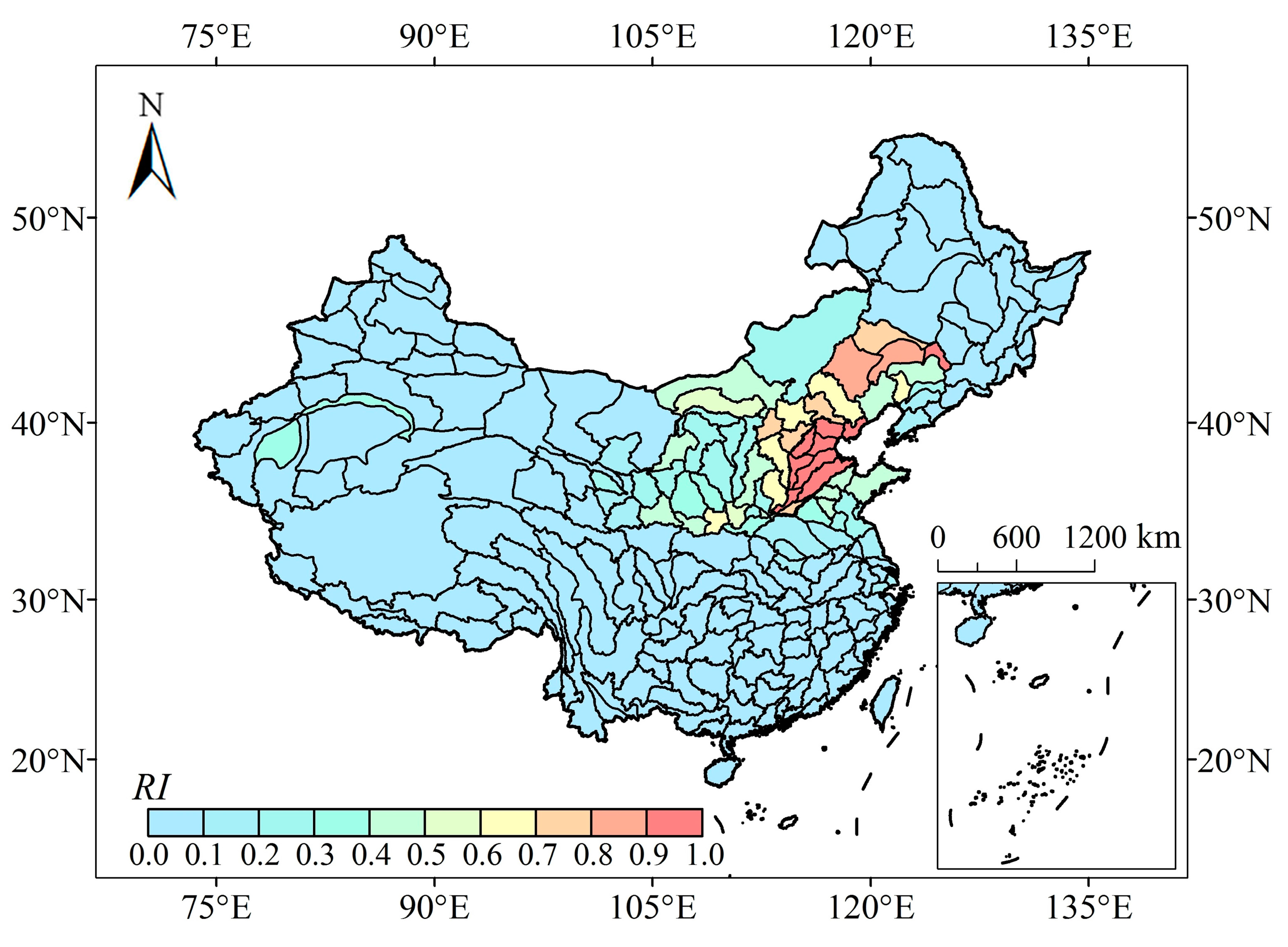
The spatial distribution of the RI in China is shown in Figure 3. The spatial variability of the WER in China is very obvious. Regions with high RI were mainly distributed in North China, which was notably higher than that in other parts of China. The WER in the Hai and Liao River Basins was the highest, with RI generally reaching more than 0.7, especially in the eastern parts of the Hai River Basin (RI > 0.9). Simultaneously, catchments in the Songhua River Basin, northwestern China, southern China, and Qinghai-Tibet Plateau had a low WER (RI < 0.4). Furthermore, the two catchments in the Northwestern River Basin had a relatively high WER compared with that of the surrounding areas. Overall, the WER was low, except in North China.

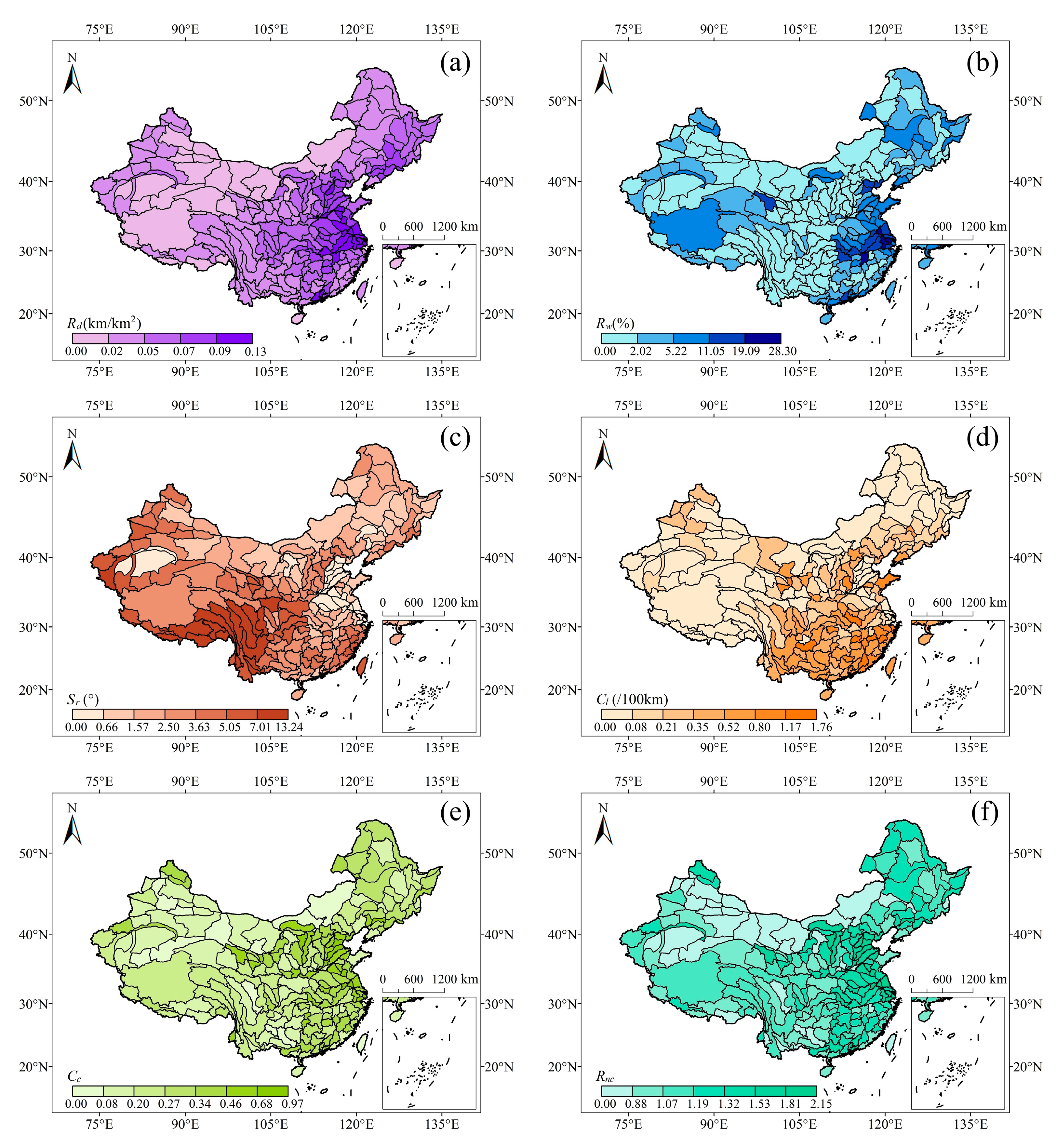
Figure 4 shows the spatial distributions of the six SCCs. R_d increased from 0.00–0.05 km/km² in the northwest inland to above 0.09 km/km² in Southeast China, among which the R_d in the estuary of the Pearl River and Yangtze River Deltas attained greater than 0.09 km/km² (Figure 4a). R_w was higher on the east coast, especially in the plain area of the lower reaches of the Yangtze River, and in lake distribution areas such as the Qinghai Lake and the hinterland of the Qinghai-Tibet Plateau (Figure 4b). R_d and R_w have similar spatial distribution characteristics in the southeast China. The values of S_r ranged from 0.0° to 13.2° in China and were the largest at the edge of the Qinghai-Tibet Plateau, while those were smaller in North China, Central China, the Northeast Plain, and the Middle-Lower Yangtze River Plain (Figure 4c). The longitudinal connectivity in the south was significantly weaker than that in the north, especially in the south of the Yangtze River Basin, with a maximum C_l value of 1.76/100 km, which indicated the weakest longitudinal connectivity (Figure 4d). Simultaneously, the C_l in the Yellow River Basin showed a spatial difference. The C_c and R_nc showed no significant regional differences in China and were relatively large in the Yellow River Basin, the Middle-Lower Yangtze River, and the estuary of the Yangtze and Pearl Rivers (Figure 4e,f) with the range, mean value, and variance of C_c and R_nc being 0.00–0.97, 0.30 and 0.18, 0.00–2.15, 1.11 and 0.47, respectively. Generally, R_d, R_w, and C_l showed high values in the east and low values in the west, whereas S_r showed a decreasing trend from the southwest to northeast. The spatial distributions of C_c and R_nc were relatively uniform in China. Additionally, the values of all six SCCs in some catchments in the western Northwest China were relatively high compared to that of the surrounding regions.

3.2. Correlation between WER and SC

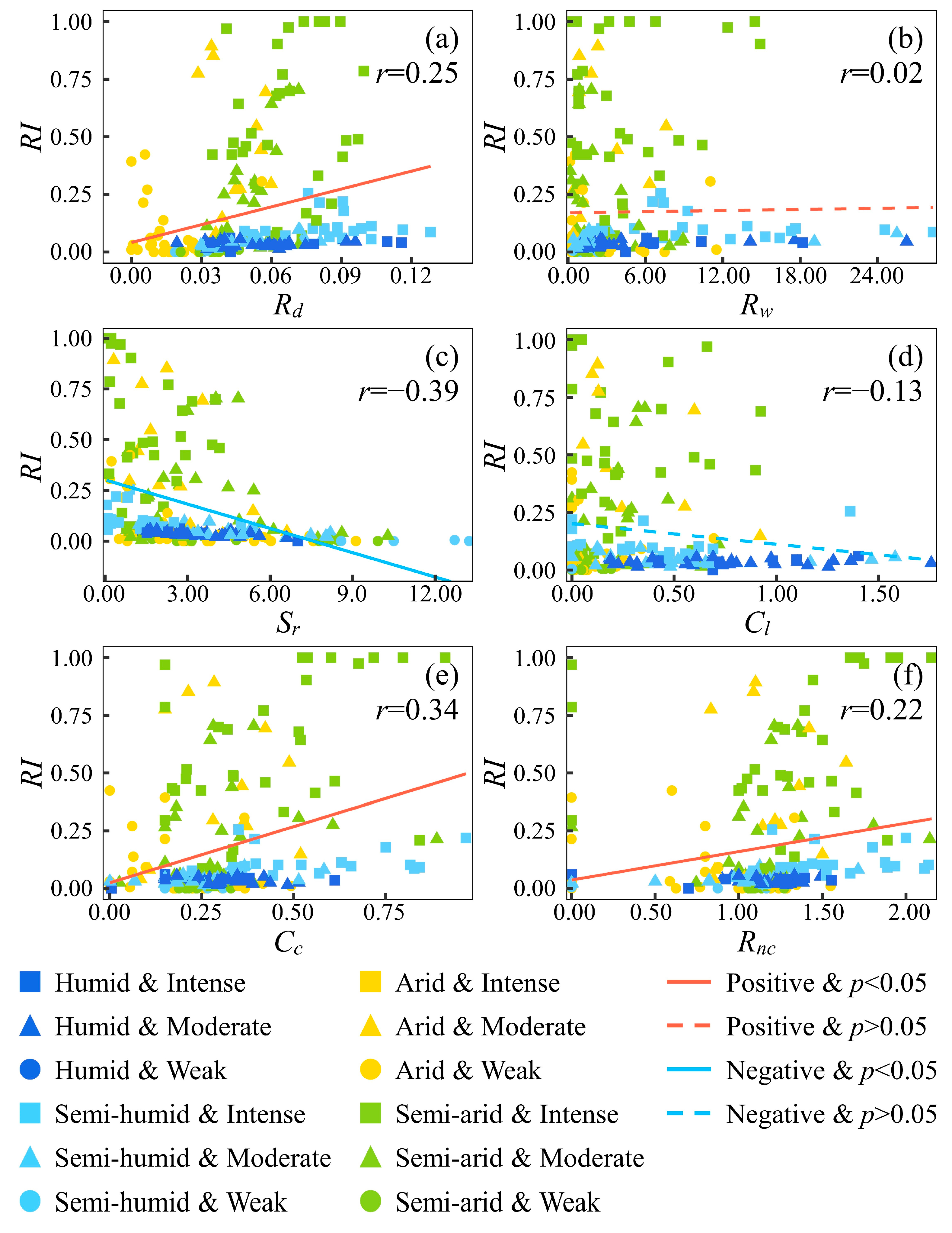
The relationship between WER and SC was relatively complex, with both positive and negative Pearson correlation coefficients (Figure 5). At the national scale, S_r and C_l were negatively correlated with WER, especially S_r, which had the strongest correlation (r = −0.39). Conversely, R_d, C_c, and R_nc were positively correlated with WER, with C_c having the strongest correlation (r = 0.34). Furthermore, R_w and C_l showed a non-significant correlation with WER, and the correlation between R_w and WER was very weak (r = 0.02). Generally, the results of the correlation analysis showed that the six SCCs had a certain impact on WER, but the impact was limited at the national scale.

GRA was applied to determine the quantitative relationship between WER and SCCs and to further reveal the relationship between WER and SC. According to the results of the cluster analysis, the GRAI between WER and SCCs was calculated for different climate and human activity intensity zones (Figure 6), and the average GRAI was calculated for each SCC nationwide (

Table 3. The GRAI between RI and each SCC nationwide.

	Rd	Rw	Sr	Cl	Cc	Rnc
GRAI	0.64	0.64	0.58	0.68	0.67	0.60

). Figure 6 and Table 3 show that the GRAI between WER and the six SCCs in each climatic and human activity intensity zone and nationwide was generally greater than the distinguishing coefficient (ρ = 0.5), which indicated that there was a strong correlation between WER and SC. Additionally, at the national scale, the GRAI between RI and each SCC had small difference (ranging from 0.58 to 0.68) and could be sorted as C_l > C_c > R_d = R_w > R_nc > S_r according to the GRAI. The C_l and C_c had relatively the strongest correlation with WER compared with other SCCs, and the GRAI were 0.68 and 0.67, respectively. R_d and R_w had an equivalent degree of correlation with WER nationwide (GRAI = 0.64), while R_nc and S_r showed a relatively weak correlation. These results indicate that the WER was evenly related to the SC, and the effect of C_l and C_c on WER was stronger than those of the other SCCs at the national scale.

3.3. Regional Variability of the Relationship between WER and SC

The correlation between WER and SC increased and showed a great difference when climatic conditions and human activity intensity were considered (

Table 4. Pearson correlation coefficient (r) between WER and SCCs in different climatic zones.

Climatic Zones	r
	Rd	Rw	Sr	Cl	Cc	Rnc
Humid	0.14	0.42 *	−0.74 *	0.06	−0.06	−0.08
Semi-humid	0.61 *	0.34 *	−0.66 *	0.01	0.59 *	0.55 *
Semi-arid	0.54 *	0.26 *	−0.46 *	0.16	0.53 *	0.29 *
Arid	0.35 *	0.03	−0.42 *	0.22	0.21	0.24
Nationwide	0.25 *	0.02	−0.39 *	−0.13	0.34 *	0.22 *

Note: * indicate p < 0.05.

and

Table 5. Pearson correlation coefficient (r) between WER and SCCs in different human activity intensity zones.

Human Activity Intensity Zones	r
	Rd	Rw	Sr	Cl	Cc	Rnc
Intense	−0.15	−0.31 *	−0.22	−0.30 *	0.17	0.04
Moderate	−0.04	−0.10	−0.27 *	−0.24 *	0.15	0.14
Weak	−0.29 *	0.03	−0.45 *	0.07	−0.27	−0.20
Nationwide	0.25 *	0.02	−0.39 *	−0.13	0.34 *	0.22 *

Note: * indicate p < 0.05.

). For example, the r of S_r increased to more than 0.66 in the humid and semi-humid zones. R_w was significantly correlated with WER in different zones, in contrast to the national scale, whereas the correlation of C_l was still non-significant. Simultaneously, R_d, R_w, and C_l showed opposite correlations in climatic and human activity intensity zones. These results indicate that climate and human activity significantly influenced the relationship between WER and SC.

The results of the GRA also confirmed the influence of climate and human activities on the relationship between WER and SC. As shown in

Table 6. Average GRAI of the different climatic and human activity intensity zones.

	Climatic Zones				Human Activity Intensity Zones
	Humid	Semi-Humid	Semi-Arid	Arid	Intense	Moderate	Weak
GRAI	0.69	0.67	0.68	0.65	0.60	0.53	0.62

, the WER in different zones differed from the average GRAI of the six SCCs. The average grey relational degrees could be sorted as humid > semi-arid > semi-humid > arid in climatic zones; however, the value of GRAI showed a small difference. Similarly, the average grey relational degrees could be sorted as weak > intense > moderate in the human activity intensity zones, which indicated that the correlation between WER and SC may first decrease and then increase with an increase in human activity intensity.

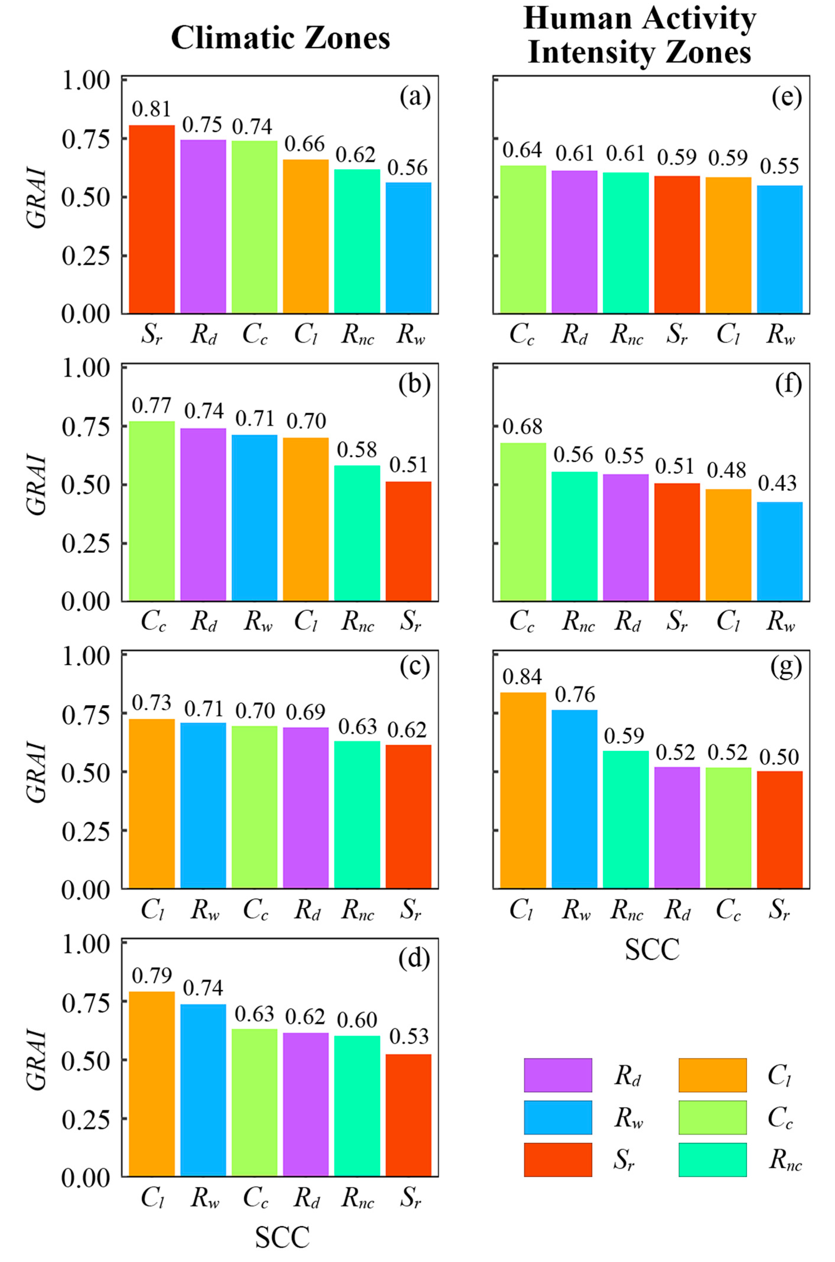
The main SCCs that affected the WER were different in the different zones (Figure 6). For different climatic zones (Figure 6a–d), S_r had the strongest grey relational degree in humid zones and the weakest in other climatic zones. R_d and C_c showed a relatively strong correlation in humid and semi-humid zones (GRAI > 0.74), while R_w was more important in semi-humid zones. The correlation between R_nc and WER was weak in all four climatic zones. The order of importance of different SCCs on WER was the same in semi-arid and arid zones; furthermore, the difference in grey relational degree between each characteristic and the WER of arid zones was more obvious.

Similarly, the main SCCs also differed across human activity intensity zones (Figure 6e–g). C_c, R_d, and R_nc were relatively important in the intense and moderate zones, whereas Sr, C_l, and R_w had a low grey relational degree, especially C_l and R_w in moderate zones. Simultaneously, the GRAI of each SCC exhibited minimal differences in the intense zones (ranging from 0.55 to 0.64). Contrastingly, the GRAI of each SCC varied greatly in the weak human activity intensity zone. Compared with the other SCCs, C_l showed the strongest correlation (GRAI = 0.84), followed by R_w (GRAI = 0.76). Summarily, the relationship between WER and SC showed regional variability under the influence of climate and human activity.

4. Discussion

4.1. Spatial Variability of WER in China

In this study, the WPL was used to reflect the WER at the catchment scale. The results showed that the WER had an obvious spatial variability in China. This result is reasonable because China also has significant spatial differences in terms of climate, human activities, stream network systems, industrial and agricultural development, etc. Several studies reported spatial differences in water pollution levels and risks. Compared with other parts of China, North China and some parts of Northeast China have a higher water pollution risk and greater water pollution pressure [66,67,68]. Cai et al., found that provinces located on the northern and central coasts had relatively higher water pollution levels [66]. Ouyang et al. reported a high potential risk of pesticide pollution in Henan, Shandong, Hebei, and Beijing [69]. Wang et al., stated that river pollution was spatially uneven and clustered in China, and the most serious water pollution occurred in the Huai, Hai, Yellow, and Liao River Basins [67].

Although only two common water pollutants (i.e., nitrogen and phosphorus) were used to evaluate WER in this study, the spatial distribution of WER was similarly mapped with those in earlier studies that used the annual provincial data of total wastewater discharge with more than 10 pollutants [66]. Compared with earlier studies, this study carried out a reasonable and reliable nationwide WER with higher resolution, which provided an opportunity to explore the relationship between WER and SCCs.

4.2. Complex Relationship between WER and SC

The results of the correlation analysis and GRA suggest that the relationship between WER and SC is relatively close in China. Earlier studies showed that SC had a significant impact on water quality [10,11,19,70]. Generally, pollutants are collected by tributaries, and transported, diluted, and deposited in streams and lakes [71], and such capability is highly related to the structure and connectivity of regional and/or large-scale stream network [11]. On the one hand, water bodies have the capacity of carrying and diluting pollutants, and the concentrations of pollutants can be changed by a series of physical, chemical, and biological processes within water bodies [14]. When the pollutant load exceeds the self-purification capacity of the water body, the water quality deteriorates, resulting in a high environmental risk. To a certain extent, the number and area of water bodies reflect the ability to resist water quality deterioration in catchments. On the other hand, rivers are important channels for pollutants transfer, and SC can reflect the ability and possibility of pollutant transmission in water bodies [55,72]. The close relationship between the SCCs and water quality is reflected in the role of flow paths, water delivery patterns, and the hydrological cycle upstream and downstream of pollutant transfer [11,16].

The correlation between the WER and SC is very complex. In this study, S_r showed a negative relationship with WER both at the national and regional scales of climate and human activities, indicating that the increase in hydrodynamic forces was helpful in reducing the WER. This result is supported by those of the earlier studies. A case in South Korea suggested that S_r was always negatively associated with total phosphorus at both sub-watershed and buffer scales [18]. You et al., stated that better hydrodynamic conditions were conducive to the migration of pollutants, i.e., catchments with steeper slopes usually had better water quality [30]. The Pearson correlation coefficients of R_d, R_w, C_l, C_c, and R_nc with WER were both positive and negative in different zones. The C_l reflected the impact of dams on water quality. A case in Turkey showed that some nitrate and phosphate values decreased significantly after dam operation, while other pollutants did not change significantly [73]. Dams also had adverse effects on water quality, for example, Dębska et al., found that water in the Utrata River below the dam reservoir showed higher values of chemical oxygen demand (COD_Mn) than that above the reservoir [74]. Simultaneously, it was generally believed that higher R_d, C_c, and R_nc created a greater possibility for the transfer of water pollutants and was beneficial to water quality. However, our results showed that R_d, C_c, and R_nc did not always have a beneficial impact on water quality, with a positive Pearson correlation coefficient in some zones, which indicated that the water quality became worse with increasing R_d, C_c, and R_nc. The response relationship is complex. Haidary et al. reported that NO₂⁻ concentration was significantly positively correlated with river density [75], and Deng stated that the concentration of several pollutants showed a negative relationship with river density, while that for others was positive [11]. For C_c and R_nc, earlier studies reported that the relationship between connectivity and water pollution level was both positive and negative [14,56,76]. The water surface ratio was an important factor for water quality at the catchment scale or smaller spatial scale [11,77], although it showed a weak correlation with the WER in this study at the national and regional scales. R_w was the dominant explanatory variable at the 100 m buffer within a 1 km upstream scale in the Han River basin, South Korea [18]. Deng stated that the influences of different water body types on water quality were discrepant, which was caused by the different purification processes of rivers and lakes [14]. The impact of water body type may be overlooked at larger spatial scales, such as national or regional scales, and should be further studied.

4.3. Regional Variation of the Influences of Climate and Human Activities

Earlier studies reported that climatic and anthropogenic factors have a significant impact on the water quality [27,28,78].

Table 7. Pearson correlation coefficient (r) and gray relational degree index (GRAI) between WER and climate, and WER and human activities nationwide.

	Climate	Human Activities
r	−0.29 *	0.47 *
GRAI	0.48	0.60

Note: * indicate p < 0.05.

showed the r and GRAI between WER and climate, and WER and human activities. The results confirmed the important impacts of climate and human activities on WER. Compared with the value of r and GRAI between WER and each SCC, the results indicated that the influences of climate and human activities were relatively moderate. In this study, the different relationship between WER and SC were shown in each climate and human activity intensity zone. There was a significant difference in the importance of S_r and R_w in climate zones (i.e., S_r was the most important in humid zones, while it was the least important in other zones, and R_w was the most important in more arid regions). R_d and C_c were more important in the humid and semi-humid zones. A possible explanation is that, compared with the carrying capacity of water for pollutants, the migration level of pollutants had a greater impact on WER for regions with abundant water. Contrastingly, for regions with relatively scarce water resources, the increase in water resource quantity had a greater impact on water pollution control [79] and thus, R_w was more important in these regions. Similarly, the construction of dams and other water conservancy projects altered the fluxes of rivers, affected the self-purification capacity of water bodies and the allocation of water resources [55,73,80,81], and played a key role in semi-arid and arid zones. The dams and reservoirs could create serious damage to river connectivity [82] and could reduce the water for ecological restoration, and the decrease in water resources resulting in water quality deterioration [79]. R_nc had low importance in all climatic zones, which was similar to that of the findings in the Southern Jiangsu Plain [11].

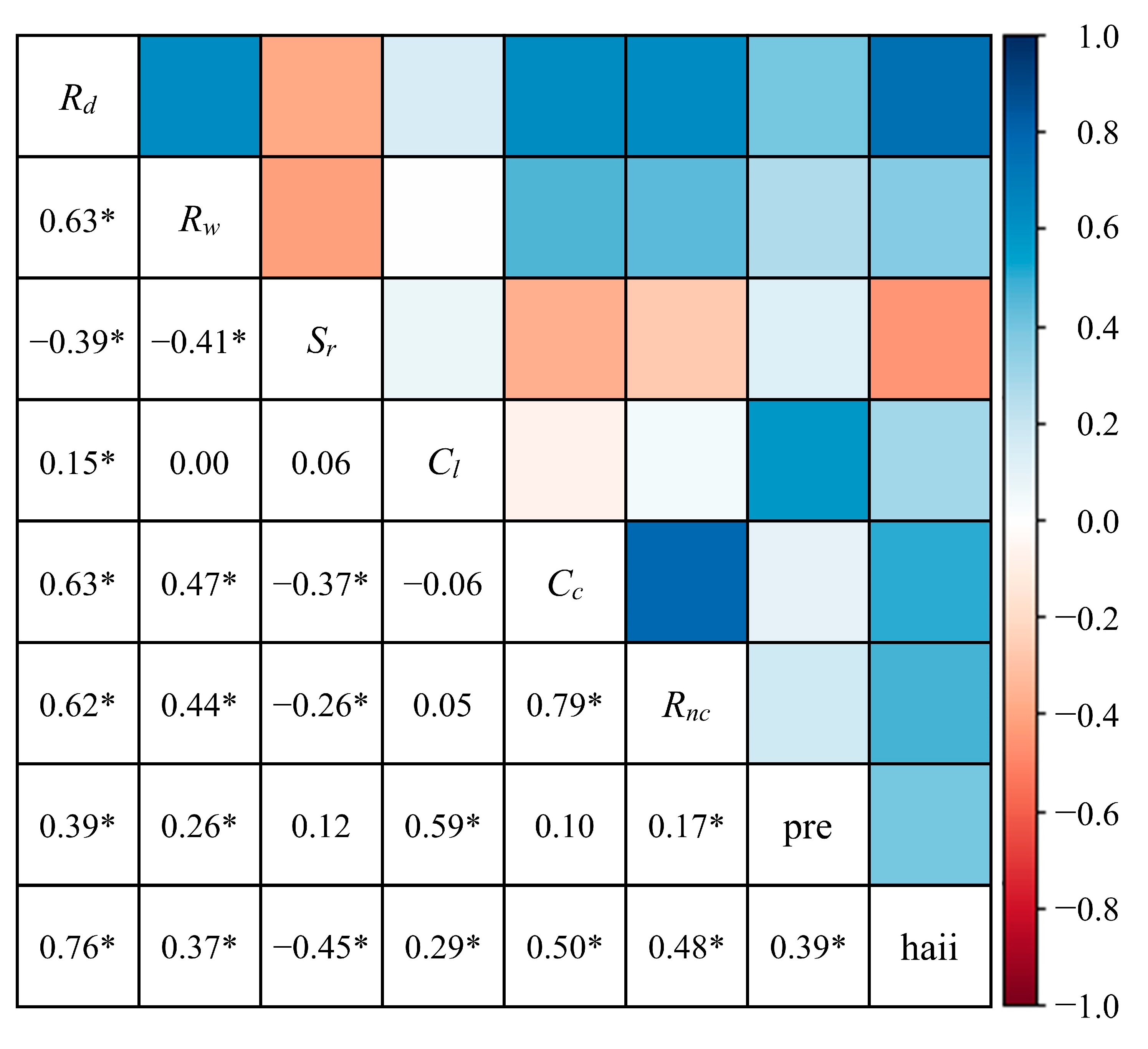
China has experienced dramatic rapid development, and high urbanization and intense human activities have influenced the natural structure and connectivity of stream networks and water quality [83,84,85], thereby affecting the relationship between WER and SC. In the intense and moderate human activity intensity zones, the importance rank of SCCs was significantly different from those of the weak zones, and the GRAI value was smaller. It indicates that human activities may have weakened the effects of SC on WER, which is the same as that in earlier studies [86]. More importantly, our results further clarified that the correlation between WER and SC was not weakened monotonically with an increase in human activity intensity, but first weakened and then enhanced. Simultaneously, Liu et al. and Gao et al. found that human factors have a greater impact on water quality than those of natural factors in the Taihu Basin with a high intensity of human activities [86,87]. Therefore, it is reasonable that R_nc, R_d, and C_c, which are highly related to human activity intensity (Figure 7), have relatively important effects on WER in intense and moderate zones. The spatial distribution of zones with weak human activity intensity was similar to that of arid zones, showing a similar relationship.

In this study, the WER was estimated using WPL, and its response to SC was analyzed using correlation analysis and GRA at the national and regional scales. Most studies used the concentrations of several pollutants to analyze the effect of SC [11,14,16], while an RI was used in this study, which was calculated using the water pollution levels of nitrogen and phosphorus. However, these pollutant concentration data were difficult to obtain nationally; thus, the RI provided a simple and accessible method to describe water quality and its response to SC. Earlier studies confirmed that the correlation between WER and SC was affected by the study scale, and that the main driving factors varied at different spatial scales [25,72,88]. Compared with earlier studies focusing on catchment scale or even smaller scale, this study analyzed the relationship between WER and SC on a larger scale (i.e., national scale, climate zone scale, and human activity intensity zone scale). Additionally, the relationship between WER and SC may be nonlinear; therefore, our results analyzed by the GRA may be more reasonable than those using the linear analysis method [11,25,89]. However, there was a strong correlation between the SCCs, climate, and human activity intensity (Figure 7), which may lead to inaccurate importance order identification. Many studies suggested that machine learning was an effective method to address the collinearity and nonlinearity issues and was applied to quantify the contribution of driven factors in many study fields [50,90,91]. However, as a data-driven method, machine learning lacks consideration of physical mechanisms. Thus, combination of machine learning with other physically-based methods could be and an effective and complementary way to better quantitatively identify the importance of influencing factors on WER in future research.

5. Conclusions

This study indicated that the WER was closely related to the SC, and confirmed the important effect of climate and human activities on the relationship between WER and SC. The relationship between WER and SC showed remarkable regional variability due to the significant impact of climate and human activities. This study systematically quantified the relationship between WER and SC on large spatial scale and emphasized the important role of regional analysis in understanding the complex relationship between WER and SC, especially under different climate and human activity intensity zones. Moreover, this study further clarified that the increase in human activity intensity would not continuously weaken the correlation between WER and SC, but first weakened and then enhanced. However, as the WER is affected by the co-impact of SC, climate, and human activities, a systemic understanding of the relationship between WER and SC requires further consideration of the nonlinearity and collinearity among driving factors. The results emphasize the important role of SC in the WER and the regional variability of their correlation in China. This study highlights that local conditions should be fully considered in WER management and differential management policies should be proposed for various catchments.

References

- Chen, S.S.; Kimirei, I.A.; Yu, C.; Shen, Q.; Gao, Q. Assessment of urban river water pollution with urbanization in East Africa. Environ. Sci. Pollut. Res. 2022, 29, 40812–40825. [Google Scholar] [CrossRef] [PubMed]
- Romanescu, G.; Cojoc, G.M.; Sandu, I.G.; Tirnovan, A.; Dascalita, D.; Sandu, I. Pollution sources and water quality in the Bistrita Catchment (Eastern Carpathians). Rev. Chim. 2015, 66, 855–863. [Google Scholar]
- Tsoraeva, E.; Bekmurzov, A.; Kozyrev, S.; Khoziev, A.; Kozyrev, A. Environmental issues of agriculture as a consequence of the intensification of the development of agricultural industry. E3S Web Conf. 2020, 215, 2003. [Google Scholar] [CrossRef]
- Wen, Y.; Schoups, G.; van de Giesen, N. Organic pollution of rivers: Combined threats of urbanization, livestock farming and global climate change. Sci. Rep. 2017, 7, 43289. [Google Scholar] [CrossRef] [Green Version]
- Wu, L.; Qi, T.; Li, D.; Yang, H.; Liu, G.; Ma, X.; Gao, J. Current status, problems and control strategies of water resources pollution in China. Water Policy 2015, 17, 423–440. [Google Scholar] [CrossRef]
- Zhao, H.; Duan, X.; Stewart, B.; You, B.; Jiang, X. Spatial correlations between urbanization and river water pollution in the heavily polluted area of Taihu Lake Basin, China. J. Geogr. Sci. 2013, 23, 735–752. [Google Scholar] [CrossRef]
- Jiang, Y. China’s water security: Current status, emerging challenges and future prospects. Environ. Sci. Policy 2015, 54, 106–125. [Google Scholar] [CrossRef]
- Han, D.; Currell, M.J.; Cao, G. Deep challenges for China’s war on water pollution. Environ. Pollut. 2016, 218, 1222–1233. [Google Scholar] [CrossRef] [Green Version]
- Lyu, H.; Zhou, F.; Li, N. Stream order and connectivity affect phosphorus distribution in plain river network. Environ. Pollut. Bioavailab. 2020, 32, 146–153. [Google Scholar] [CrossRef]
- Yu, Z.; Wang, Q.; Xu, Y.; Lu, M.; Lin, Z.; Gao, B. Dynamic impacts of changes in river structure and connectivity on water quality under urbanization in the Yangtze River Delta plain. Ecol. Indic. 2022, 135, 108582. [Google Scholar] [CrossRef]
- Deng, X. Correlations between water quality and the structure and connectivity of the river network in the Southern Jiangsu Plain, Eastern China. Sci. Total Environ. 2019, 664, 583–594. [Google Scholar] [CrossRef]
- Huang, F.; Wang, X.; Lou, L.; Zhou, Z.; Wu, J. Spatial variation and source apportionment of water pollution in Qiantang River (China) using statistical techniques. Water Res. 2010, 44, 1562–1572. [Google Scholar] [CrossRef] [PubMed]
- Dou, M.; Yu, L.; Jin, M.; Zhang, Y. Correlation analysis and threshold value research on the form and function indexes of an urban interconnected river system network. Water Supply 2016, 16, 1776–1786. [Google Scholar] [CrossRef] [Green Version]
- Deng, X. Influence of water body area on water quality in the southern Jiangsu Plain, eastern China. J. Clean. Prod. 2020, 254, 120136. [Google Scholar] [CrossRef]
- Zhao, J.; Lin, L.; Yang, K.; Liu, Q.; Qian, G. Influences of land use on water quality in a reticular river network area: A case study in Shanghai, China. Landsc. Urban Plan. 2015, 137, 20–29. [Google Scholar] [CrossRef]
- Helton, A.M.; Hall, R.O.; Bertuzzo, E. How network structure can affect nitrogen removal by streams. Freshw. Biol. 2018, 63, 128–140. [Google Scholar] [CrossRef]
- Pratt, B.; Chang, H. Effects of land cover, topography, and built structure on seasonal water quality at multiple spatial scales. J. Hazard. Mater. 2012, 209–210, 48–58. [Google Scholar] [CrossRef]
- Mainali, J.; Chang, H. Landscape and anthropogenic factors affecting spatial patterns of water quality trends in a large river basin, South Korea. J. Hydrol. 2018, 564, 26–40. [Google Scholar] [CrossRef]
- Mazur, M.L.C.; Smith, B.; Bird, B.; McMillan, S.; Pyron, M.; Hauswald, C. Hydrologic connectivity and land cover affect floodplain lake water quality, fish abundance, and fish diversity in floodplain lakes of the Wabash-White River basin. River Res. Appl. 2022, 38, 160–172. [Google Scholar] [CrossRef]
- Seo, J.; Won, J.; Choi, J.; Kim, S. Identification of the Relative Importance of Factors Affecting the Spatial Variability of River Water Quality. Sustainability 2021, 13, 11319. [Google Scholar] [CrossRef]
- Knoll, L.B.; Hagenbuch, E.J.; Stevens, M.H.; Vanni, M.J.; Renwick, W.H.; Denlinger, J.C.; Hale, R.S.; González, M.J. Predicting eutrophication status in reservoirs at large spatial scales using landscape and morphometric variables. Inland Waters 2015, 5, 203–214. [Google Scholar] [CrossRef]
- Grizzetti, B.; Pistocchi, A.; Liquete, C.; Udias, A.; Bouraoui, F.; van de Bund, W. Human pressures and ecological status of European rivers. Sci. Rep. 2017, 7, 205. [Google Scholar] [CrossRef] [PubMed] [Green Version]
- Liu, B.; Cai, S.; Wang, H.; Cui, C.; Cao, X. Hydrodynamics and water quality of the Hongze Lake in response to human activities. Environ. Sci. Pollut. Res. 2021, 28, 46215–46232. [Google Scholar] [CrossRef] [PubMed]
- Michalak, A.M. Study role of climate change in extreme threats to water quality. Nature 2016, 535, 349–350. [Google Scholar] [CrossRef] [Green Version]
- Shi, W.; Xia, J.; Zhang, X. Influences of anthropogenic activities and topography on water quality in the highly regulated Huai River basin, China. Environ. Sci. Pollut. Res. 2016, 23, 21460–21474. [Google Scholar] [CrossRef]
- Yu, S.; Xu, Z.; Wu, W.; Zuo, D. Effect of land use types on stream water quality under seasonal variation and topographic characteristics in the Wei River basin, China. Ecol. Indic. 2016, 60, 202–212. [Google Scholar] [CrossRef]
- Jiang, J.; Sharma, A.; Sivakumar, B.; Wang, P. A global assessment of climate–water quality relationships in large rivers: An elasticity perspective. Sci. Total Environ. 2014, 468–469, 877–891. [Google Scholar] [CrossRef]
- Kaushal, S.S.; Gold, A.J.; Bernal, S.; Tank, J.L. Diverse water quality responses to extreme climate events: An introduction. Biogeochemistry 2018, 141, 273–279. [Google Scholar] [CrossRef] [Green Version]
- Nguyen, B.T.; Vo, L.D.; Nguyen, T.X.; Quang, N.X. The interactive effects of natural factor and pollution source on surface water quality in the Lower Mekong River Basin, Southwestern Vietnam. Water Resour. 2020, 47, 865–876. [Google Scholar] [CrossRef]
- You, Q.; Fang, N.; Liu, L.; Yang, W.; Zhang, L.; Wang, Y. Effects of land use, topography, climate and socio-economic factors on geographical variation pattern of inland surface water quality in China. PLoS ONE 2019, 14, e217840. [Google Scholar] [CrossRef]
- Luo, Z.; Zuo, Q.; Gan, R.; Ma, J. Effect of human activity intensity on stream structure and connectivity in Shaying River Basin, China. Water Sci. Technol.-Water Supply 2018, 18, 754–766. [Google Scholar] [CrossRef]
- Ward, A.S.; Wondzell, S.M.; Schmadel, N.M.; Herzog, S.P. Climate change causes river network contraction and disconnection in the H.J. Andrews Experimental Forest, Oregon, USA. Front. Water 2020, 2, 7. [Google Scholar] [CrossRef]
- Cheng, S.; Cheng, L.; Liu, P.; Qin, S.; Zhang, L.; Xu, C.Y.; Xiong, L.; Liu, L.; Xia, J. An analytical baseflow coefficient curve for depicting the spatial variability of mean annual catchment baseflow. Water Resour. Res. 2021, 57, e2020WR029529. [Google Scholar] [CrossRef]
- Ye, L.; Cheng, L.; Liu, P.; Liu, D.; Zhang, L.; Qin, S.; Xia, J. Management of vegetative land for more water yield under future climate conditions in the over-utilized water resources regions: A case study in the Xiong’an New area. J. Hydrol. 2021, 600, 126563. [Google Scholar] [CrossRef]
- Kreiling, R.M.; Thoms, M.C.; Bartsch, L.A.; Richardson, W.B.; Christensen, V.G. Complex Response of Sediment Phosphorus to Land Use and Management Within a River Network. J. Geophys. Res. Biogeosci. 2019, 124, 1764–1780. [Google Scholar] [CrossRef]
- Ranjbar, S.; Hooshyar, M.; Singh, A.; Wang, D. Quantifying climatic controls on river network branching structure across scales. Water Resour. Res. 2018, 54, 7347–7360. [Google Scholar] [CrossRef]
- Li, Y.; Cao, J.; Shen, F.; Xia, J. The changes of renewable water resources in China during 1956–2010. Sci. China Earth Sci. 2014, 57, 1825–1833. [Google Scholar] [CrossRef]
- He, J.; Yang, K.; Tang, W.; Lu, H.; Qin, J.; Chen, Y.; Li, X. The first high-resolution meteorological forcing dataset for land process studies over China. Sci. Data 2020, 7, 25. [Google Scholar] [CrossRef] [Green Version]
- Sanderson, E.W.; Jaiteh, M.; Levy, M.A.; Redford, K.H.; Wannebo, A.V.; Woolmer, G. The human footprint and the last of the wild. Bioscience 2002, 52, 891–904. [Google Scholar] [CrossRef] [Green Version]
- Liu, C.; Kroeze, C.; Hoekstra, A.Y.; Gerbens-Leenes, W. Past and future trends in grey water footprints of anthropogenic nitrogen and phosphorus inputs to major world rivers. Ecol. Indic. 2012, 18, 42–49. [Google Scholar] [CrossRef]
- Mekonnen, M.M.; Hoekstra, A.Y. Global gray water footprint and water pollution levels related to anthropogenic nitrogen loads to fresh water. Environ. Sci. Technol. 2015, 49, 12860–12868. [Google Scholar] [CrossRef] [PubMed]
- Mekonnen, M.M.; Hoekstra, A.Y. Global anthropogenic phosphorus loads to freshwater and associated grey water footprints and water pollution levels: A high-resolution global study. Water Resour. Res. 2018, 54, 345–358. [Google Scholar] [CrossRef] [Green Version]
- Hoekstra, A.Y. Human appropriation of natural capital: A comparison of ecological footprint and water footprint analysis. Ecol. Econ. 2009, 68, 1963–1974. [Google Scholar] [CrossRef] [Green Version]
- Feng, H.; Sun, F.; Liu, Y.; Zeng, P.; Deng, L.; Che, Y. Mapping multiple water pollutants across China using the grey water footprint. Sci. Total Environ. 2021, 785, 147255. [Google Scholar] [CrossRef] [PubMed]
- Carey, R.O.; Hochmuth, G.J.; Martinez, C.J.; Boyer, T.H.; Dukes, M.D.; Toor, G.S.; Cisar, J.L. Evaluating nutrient impacts in urban watersheds: Challenges and research opportunities. Environ. Pollut. 2013, 173, 138–149. [Google Scholar] [CrossRef] [PubMed]
- Ma, J.; Chen, X.; Huang, B.; Shi, Y.; Chi, G.; Lu, C. Utilizing water characteristics and sediment nitrogen isotopic features to identify non-point nitrogen pollution sources at watershed scale in Liaoning Province, China. Environ. Sci. Pollut. Res. 2015, 22, 2699–2707. [Google Scholar] [CrossRef]
- Zhao, Z.; Qin, W.; Bai, Z.; Ma, L. Agricultural nitrogen and phosphorus emissions to water and their mitigation options in the Haihe Basin, China. Agr. Water Manag. 2019, 212, 262–272. [Google Scholar] [CrossRef]
- Chad, M.; Navin, R.; Jonathan, A.F. Farming the planet: 2. Geographic distribution of crop areas, yields, physiological types, and net primary production in the year 2000. Glob. Biogeochem. Cycles 2008, 22, GB1022. [Google Scholar]
- Hobeichi, S.; Abramowitz, G.; Evans, J.; Beck, H.E. Linear Optimal Runoff Aggregate (LORA): A global gridded synthesis runoff product. Hydrol. Earth Syst. Sci. 2019, 23, 851–870. [Google Scholar] [CrossRef] [Green Version]
- Xu, Z.; Cheng, L.; Liu, P.; Hou, Q.; Cheng, S.; Qin, S.; Liu, L.; Xia, J. Investigating the spatial variability of water security risk and its driving mechanisms in China using machine learning. J. Clean. Prod. 2022, 362, 132303. [Google Scholar] [CrossRef]
- Varis, O.; Kummu, M.; Lehr, C.; Shen, D. China’s stressed waters: Societal and environmental vulnerability in China’s internal and transboundary river systems. Appl. Geogr. 2014, 53, 105–116. [Google Scholar] [CrossRef]
- Lei, C.; Wagner, P.D.; Fohrer, N. Effects of land cover, topography, and soil on stream water quality at multiple spatial and seasonal scales in a German lowland catchment. Ecol. Indic. 2021, 120, 106940. [Google Scholar] [CrossRef]
- Turnbull, L.; Wainwright, J.; Brazier, R.E. A conceptual framework for understanding semi-arid land degradation: Ecohydrological interactions across multiple-space and time scales. Ecohydrology 2008, 1, 23–34. [Google Scholar] [CrossRef] [Green Version]
- Pekel, J.; Cottam, A.; Gorelick, N.; Belward, A.S. High-resolution mapping of global surface water and its long-term changes. Nature 2016, 540, 418. [Google Scholar] [CrossRef] [PubMed]
- Grill, G.; Lehner, B.; Thieme, M.; Geenen, B.; Tickner, D.; Antonelli, F.; Babu, S.; Borrelli, P.; Cheng, L.; Crochetiere, H.; et al. Mapping the world’s free-flowing rivers. Nature 2019, 569, 215. [Google Scholar] [CrossRef]
- Fan, X.; Cui, B.; Zhao, H.; Zhang, Z. The changes of wetland network pattern associated with water quality in the Pearl River Delta, China. Clean Soil Air Water 2012, 40, 1064–1075. [Google Scholar] [CrossRef]
- Deng, J. Introduction to Grey System Theory. J. Grey Syst. 1989, 1, 1–24. [Google Scholar]
- Li, B.; Wu, Q.; Zhang, W.; Liu, Z. Water resources security evaluation model based on grey relational analysis and analytic network process: A case study of Guizhou Province. J. Water Process. Eng. 2020, 37, 101429. [Google Scholar] [CrossRef]
- Li, X.; Li, G.; Zhang, Y. Identifying major factors affecting groundwater change in the North China Plain with Grey Relational Analysis. Water 2014, 6, 1581–1600. [Google Scholar] [CrossRef] [Green Version]
- Yang, T.; Liu, J.; Chen, Q. Assessment of plain river ecosystem function based on improved gray system model and analytic hierarchy process for the Fuyang River, Haihe River Basin, China. Ecol. Model. 2013, 268, 37–47. [Google Scholar] [CrossRef]
- Wong, H.; Hu, B.Q.; Ip, W.C.; Xia, J. Change-point analysis of hydrological time series using grey relational method. J. Hydrol. 2006, 324, 323–338. [Google Scholar] [CrossRef]
- MacQueen, J.B. Some methods for classification and analysis of multivariate observations. Berkeley Symp. Math. Stat. Probab. 1967, 5, 281–297. [Google Scholar]
- Shi, N.; Liu, X.; Guan, Y. Research on k-means Clustering Algorithm: An Improved k-means Clustering Algorithm. In Proceedings of the 2010 3rd International Symposium on Intelligent Information Technology and Security Informatics (IITSI 2010), Jinggangshan, China, 2–4 April 2010; pp. 63–67. [Google Scholar]
- Ilbay-Yupa, M.; Lavado-Casimiro, W.; Rau, P.; Zubieta, R.; Castillón, F. Updating regionalization of precipitation in Ecuador. Theor. Appl. Climatol. 2021, 143, 1513–1528. [Google Scholar] [CrossRef]
- Jiang, N.; Qian, W.; Leung, J.C. The global monsoon division combining the k-means clustering method and low-level cross-equatorial flow. Clim. Dyn. 2016, 47, 2345–2359. [Google Scholar] [CrossRef]
- Cai, J.; Varis, O.; Yin, H. China’s water resources vulnerability: A spatio-temporal analysis during 2003–2013. J. Clean. Prod. 2017, 142, 2901–2910. [Google Scholar] [CrossRef]
- Wang, E.R.; Li, Q.; Hu, H.; Peng, F.L.; Zhang, P.; Li, J.J. Spatial characteristics and influencing factors of river pollution in China. Water Environ. Res. 2019, 91, 351–363. [Google Scholar] [CrossRef]
- Yan, Y.; Zhang, Y.; Fan, B.; Yang, M.; Cai, L.; Fu, X.; Liu, X.; Hou, J. Estimation and spatial analysis of water pollution loads from towns in China. Int. J. Sustain. Dev. World Ecol. 2011, 18, 219–225. [Google Scholar] [CrossRef]
- Ouyang, W.; Cai, G.; Huang, W.; Hao, F. Temporal–spatial loss of diffuse pesticide and potential risks for water quality in China. Sci. Total Environ. 2016, 541, 551–558. [Google Scholar] [CrossRef]
- Harvey, J.; Velez, J.G.; Schmadel, N.; Scott, D.; Boyer, E.; Alexander, R.; Eng, K.; Golden, H.; Kettner, A.; Konrad, C.; et al. How hydrologic connectivity regulates water quality in river corridors. J. Am. Water Resour. Assoc. 2019, 55, 369–381. [Google Scholar] [CrossRef]
- Zhu, Q.D.; Sun, J.H.; Hua, G.F.; Wang, J.H.; Wang, H. Runoff characteristics and non-point source pollution analysis in the Taihu Lake Basin: A case study of the town of Xueyan, China. Environ. Sci. Pollut. Res. 2015, 22, 15029–15036. [Google Scholar] [CrossRef]
- Wu, J.; Jin, Y.; Hao, Y.; Lu, J. Identification of the control factors affecting water quality variation at multi-spatial scales in a headwater watershed. Environ. Sci. Pollut. Res. 2021, 28, 11129–11141. [Google Scholar] [CrossRef] [PubMed]
- Bor, A.; Elçi, Ş. Impacts of construction of dam on the flow regimes and water quality: A case study from Turkey. Int. J. Environ. Sci. Technol. 2022, 19, 4069–4086. [Google Scholar] [CrossRef]
- Dębska, K.; Rutkowska, B.; Szulc, W. The influence of a dam reservoir on water quality in a small lowland river. Environ. Monit. Assess. 2021, 193, 123. [Google Scholar] [CrossRef] [PubMed]
- Haidary, A.; Amiri, B.J.; Adamowski, J.; Fohrer, N.; Nakane, K. Assessing the impacts of four land use types on the water quality of wetlands in Japan. Water Resour. Manag. 2013, 27, 2217–2229. [Google Scholar] [CrossRef]
- Qiu, C.; Li, Y.; Wright, A.L.; Wang, C.; Xu, J.; Zhou, S.; Huang, W.; Wu, Y.; Zhang, Y.; Liu, H. Spatial effects of urban-rural ditch connectivity gradient changes on water quality to support ditch optimization and management. Sustainability 2021, 13, 8329. [Google Scholar] [CrossRef]
- Chang, L.; Cheng, L.; Huang, C.; Qin, S.; Fu, C.; Li, S. Extracting urban water bodies from Landsat imagery based on mNDWI and HSV transformation. Remote Sens. 2022, 14, 5785. [Google Scholar] [CrossRef]
- Liu, J.; Zhang, X.; Wu, B.; Pan, G.; Xu, J.; Wu, S. Spatial scale and seasonal dependence of land use impacts on riverine water quality in the Huai River basin, China. Environ. Sci. Pollut. Res. 2017, 24, 20995–21010. [Google Scholar] [CrossRef]
- Tang, W.; Mao, Z.; Zhang, H.; Shan, B.; Zhao, Y.; Ding, Y. Water resources: The prerequisite for ecological restoration of rivers in the Hai River Basin, northern China. Environ. Sci. Pollut. Res. 2015, 22, 1359–1365. [Google Scholar] [CrossRef]
- Lee, G.; Lee, H.W.; Lee, Y.S.; Choi, J.H.; Yang, J.E.; Lim, K.J.; Kim, J. The effect of reduced flow on downstream water systems due to the Kumgangsan Dam under dry conditions. Water 2019, 11, 739. [Google Scholar] [CrossRef] [Green Version]
- Wang, Q.L.; Wang, Y.P.; Zhang, L.; Qin, S.J.; Zhang, Q.; Liu, P.; Liu, L.; Zou, K.J.; Cheng, S.J.; Cheng, L. Land surface models significantly underestimate the impact of land-use changes on global evapotranspiration. Environ. Res. Lett. 2021, 16, 124047. [Google Scholar] [CrossRef]
- Michaelides, K.; Chappell, A. Connectivity as a concept for characterising hydrological behaviour. Hydrol. Process. 2009, 23, 517–522. [Google Scholar] [CrossRef]
- Han, L.; Xu, Y.; Lei, C.; Yang, L.; Deng, X.; Hu, C.; Xu, G. Degrading river network due to urbanization in Yangtze River Delta. J. Geogr. Sci. 2016, 26, 694–706. [Google Scholar] [CrossRef] [Green Version]
- Liu, S.; Fu, R.; Liu, Y.; Suo, C. Spatiotemporal variations of water quality and their driving forces in the Yangtze River Basin, China, from 2008 to 2020 based on multi-statistical analyses. Environ. Sci. Pollut. Res. 2022, 29, 69388–69401. [Google Scholar] [CrossRef] [PubMed]
- Wang, Q.; Cheng, L.; Zhang, L.; Liu, P.; Qin, S.; Liu, L.; Jing, Z. Quantifying the impacts of land-cover changes on global evapotranspiration based on the continuous remote sensing observations during 1982–2016. J. Hydrol. 2021, 598, 126231. [Google Scholar] [CrossRef]
- Liu, Y.; Zhang, H.; Zeng, P.; Wang, Y.; Li, G.; Sun, F.; Che, Y. Linking hydraulic geometry, land use, and stream water quality in the Taihu Basin, China. Environ. Monit. Assess. 2021, 193, 484. [Google Scholar] [CrossRef]
- Gao, B.; Xu, Y.; Lin, Z.; Lu, M.; Wang, Q. Temporal and spatial characteristics of river water quality and its influence factors in the Taihu Basin Plains, Lower Yangtze River, China. Water 2022, 14, 1654. [Google Scholar] [CrossRef]
- Xia, J.; Wang, L.; Yu, J.; Zhan, C.; Zhang, Y.; Qiao, Y.; Wang, Y. Impact of environmental factors on water quality at multiple spatial scales and its spatial variation in Huai River Basin, China. Sci. China Earth Sci. 2018, 61, 82–92. [Google Scholar] [CrossRef]
- Ewane, E.B. Assessing land use and landscape factors as determinants of water quality trends in Nyong River basin, Cameroon. Environ. Monit. Assess. 2020, 192, 507. [Google Scholar] [CrossRef]
- Rahmati, O.; Falah, F.; Naghibi, S.A.; Biggs, T.; Soltani, M.; Deo, R.C.; Cerdà, A.; Mohammadi, F.; Bui, D.T. Land subsidence modelling using tree-based machine learning algorithms. Sci. Total Environ. 2019, 672, 239–252. [Google Scholar] [CrossRef]
- Cheng, S.; Cheng, L.; Qin, S.; Zhang, L.; Liu, P.; Liu, L.; Xu, Z.; Wang, Q. Improved understanding of how catchment properties control hydrological partitioning through machine learning. Water Resour. Res. 2022, 58, e2021WR031412. [Google Scholar] [CrossRef]
Figure 1.
Map of the study area. The subplot (a) shows the main rivers, lakes, level-Ⅲ catchments and the digital elevation model (DEM), and (b) shows the 10 level-Ⅰ catchments in China.
Figure 2.
Maps depicting the spatial variations of (a) mean annual precipitation, (b) human activity intensity, and their clustered zones determined by the K-means clustering algorithm in (c) and (d), respectively.
Figure 3.
Map of the spatial distribution of water environment risk index (RI) in China.
Figure 4.
Maps of the spatial distributions of (a) river density (Rd), (b) water surface ratio (Rw), (c) average slope (Sr), (d) longitudinal connectivity (Cl), (e) cyclical connectivity (Cc) and (f) node connection ratio (Rnc) in China.
Figure 5.
Plots illustrating the correlation between WER and SCCs in China. The subplots (a)–(f) showed correlations between RI and Rd, RI and Rw, RI and Sr, RI and Cl, RI and Cc, RI and Rnc, respectively.
Figure 6.
Plots illustrating the grey relational degree index (GRAI) in different climatic zones (left panel) and human activity intensity zones (right panel). The subplots in left panel (a)–(d) showed GRAI of six SCCs in humid, semi-humid, semi-arid and arid zones, respectively. The subplots in right panel (e)–(g) showed GRAI of six SCCs in intense, moderate and weak zones, respectively.
Figure 7.
Plots illustrating the Pearson correlation coefficients among SCCs (i.e., Rd, Rw, Sr, Cl, Cc, and Rnc), precipitation (pre) and human activity intensity index (haii). And * indicate p < 0.05.