The Application and Improvement of Soil–Water Characteristic Curves through In Situ Monitoring Data in the Plains

Abstract

In order to study the soil–water characteristic curve and soil–water movement in the unsaturated zone of the humid plain area and investigate its influence on the regional water cycle process, this study conducted a long series of hydrometeorological data monitoring on the whole process of precipitation, evaporation, soil water content, pore water pressure and depth of groundwater level at the Jintan field hydrological test in the plain area of the Taihu Basin, China. Based on the collected data, the soil water dynamic at different depths was analyzed, and the results showed that the soil water fluctuated most frequently and drastically at a soil horizon depth of 0–40 cm, with an obvious soil moisture wetting and drying cycle. The van Genuchten model (VG model) was used to describe the soil–water characteristic curve, and the parameters of the VG model were obtained by numerical inversion of field monitoring data using numerical code (HYDRUS-1D). The obtained parameters were used to simulate soil water movement in each soil horizon for six precipitation events and were compared with the simulation results of laboratory data. The study shows that the soil water simulation based on field data is better, which verifies the accuracy and reliability of the VG model obtained from field observation and provides a reliable theoretical basis for soil water movement and the calculation of runoff yield in the plain area of the Taihu Basin.

1. Introduction

Plain areas have always been developed agricultural regions due to the abundant water resources [1,2]. In order to ensure regional agricultural production and security, agricultural water is an important issue for regional water resources management [3,4], and the movement and presence of soil water is a scientific guarantee for efficient water use in agriculture [5,6]. The unsaturated zone is the area of soil that contains both air and moisture [7,8], where the root system of crops mostly grows. Water movement in the unsaturated zone is one of the key parts of the agricultural water cycle [9]. Research on SWCC of the unsaturated zone helps improve soil water utilization efficiency [10,11] to realize the sustainable development of regional water resource management. Meanwhile, the frequent extreme weather due to global climate change and the underlying surface changes caused by human activities have greatly affected the terrestrial hydrological cycle. The plain river network in eastern China is characterized by flat terrain and shallow groundwater. Floods are prone to occur during the rainy season, affecting the safety of people’s lives and property [12]. Mastering the mechanism of soil water movement in the unsaturated zone in this region is the key to studying the hydrological cycle characteristics and runoff generation mechanisms, which is of great significance for regional flood control forecasting and risk management [13,14].

The unsaturated zone connects surface water and groundwater and is a key part of the hydrological cycle [15,16,17]. The soil–water characteristic curve (SWCC) reflects the most basic characteristics of water in the unsaturated zone and is extremely critical for studying the existence and movement of soil water [18,19]. The SWCC represents the relationship between soil water content and pore water pressure [20,21] and is affected by many factors, such as soil texture, structure, bulk density, organic content and particle size distribution [22,23]. Many methods for measuring SWCC have been developed. Common laboratory methods for measuring pore water pressure include the pressure plate apparatus [24], the dew point potential meter method [25], and the filter paper method [26]. Common soil water content determination methods include the drying method, neutron method and ray method, all of which are determined by measuring a specific series of soil water content and their corresponding soil pressure, and then the corresponding empirical model is used to simulate the measured data series to obtain the SWCC. However, most of these methods have shortcomings, such as being time-consuming, high cost, limited range, inaccuracies and soil susceptibility to disturbance [27]. Therefore, some scholars have proposed an indirect estimation method to replace direct laboratory measurement [28]. This method estimates SWCC indirectly, mainly by establishing empirical relationships for basic soil parameters that are relatively easy to obtain. For example, predictions based on the basic physical properties of the soil combined with regression analysis [29,30], artificial neural network [31] and other pure mathematical methods are also based on the basic physical properties of the soil sample, such as bulk density, particle size distribution [32], using fractal theory to predict SWCC [33]. The basic soil properties data used for the indirect prediction method are mainly obtained in the laboratory and cannot represent the actual conditions in the field. The prediction accuracy and reliability of most indirect methods are only evaluated based on the statistical analysis of the measured data, and the predictions may not be appropriate for specific problems [34].

In recent years, many scholars have performed numerical inversion of the soil–water characteristic curve parameters and obtained SWCCs with strong adaptability. The common models for obtaining SWCC include the Brooks–Corey [35,36], van Genuchten [37], and Gardner–Russo models [38,39]. This method is more convenient, flexible and better suited to complex and variable soil conditions. However, in the current study, which is mainly reliant on laboratory data, Whisler and Zachmann [40,41] matched simulated and measured values of soil drainage flow to estimate the unsaturated hydraulic conductivity, and Šimůnek et al. [42] used the tension disk infiltration data for numerical inversion to derive parameters of soil-hydraulic characteristic, but these methods have not been validated by field experiments. Dane et al. [43] artificially controlled the upper boundary conditions in the field for the numerical inversion of SWCC parameters. In fact, the field soil conditions are very complex, and the temporal and spatial variability of soil properties makes it impossible to perfectly simulate under simple conditions. Therefore, the inversion of SWCC parameters for complex field soil profiles under natural conditions requires further research.

The study established a hydrological field test in Baitaqiao (BTQ), Jintan, Taihu Basin, to monitor basic hydrometeorological elements. Based on the field monitoring data, the VG model parameters at different depths were numerically inversed using HYDRUS-1D, and the rationality of the obtained parameters was analyzed. Then, the model was used to simulate precipitation events and obtain the soil water movement for each precipitation event. The simulation results were compared and analyzed with the results obtained from laboratory measurements to evaluate the accuracy and reliability of the SWCC model based on field observations. The exploration and application of this method can provide a basis for revealing the theoretical connection between soil water content and suction and further improve the hydrodynamic theory of unsaturated zones of plains.

2. Materials and Methods

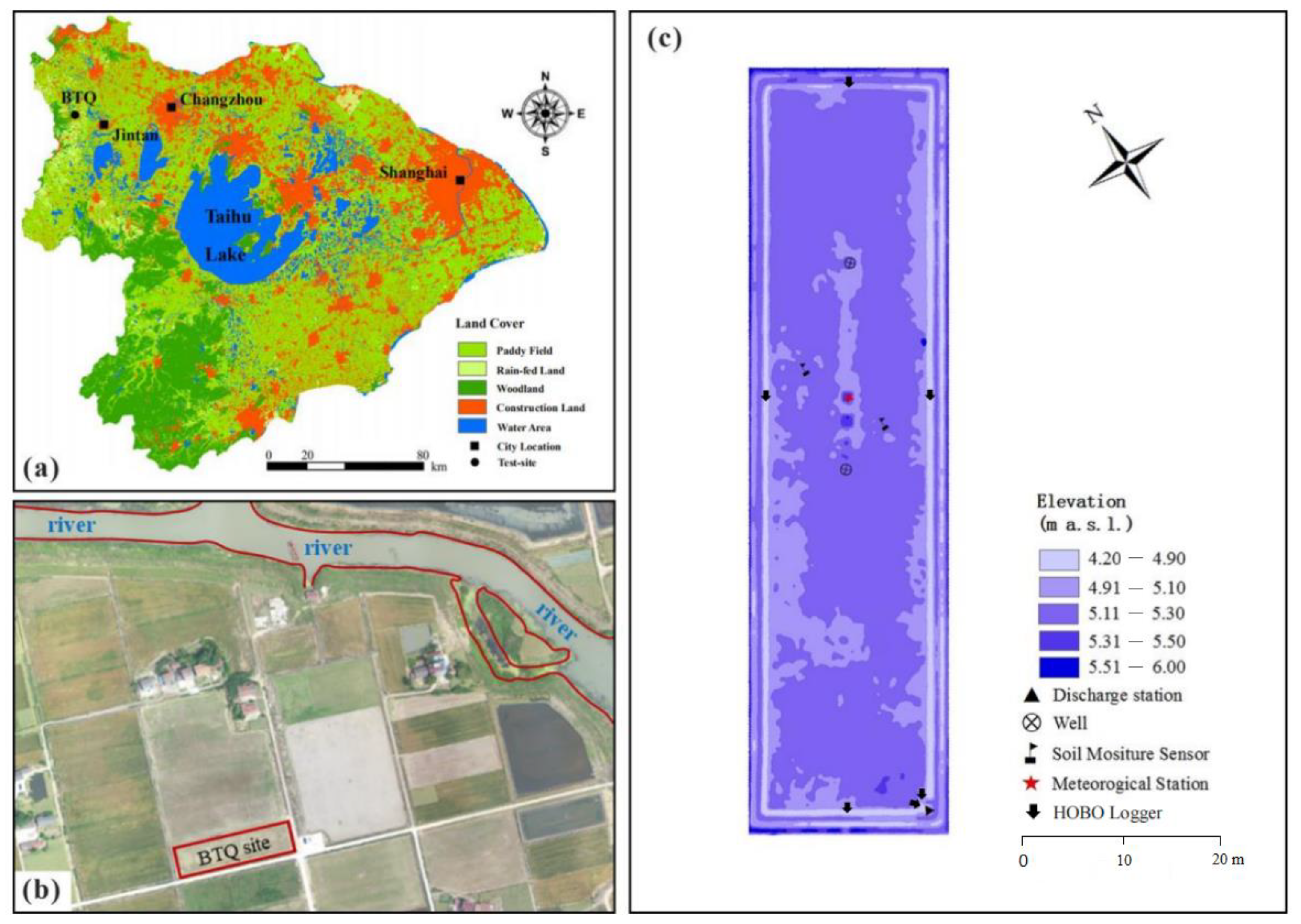
2.1. Study Area

The data were acquired in a field in southern Jiangsu, China, which has a subtropical climate with an average annual precipitation of 1070 mm, which is mainly concentrated from April to September each year. The mean annual temperature is 15.3 °C, and the mean annual evaporation is 1283.1 mm. The field study was conducted in a hydrologically isolated test site, which is a typical flat lowland surrounded by ditches in the Taihu Basin.

The BTQ field is located in Zhiqian, Jintan and Changzhou (31.760° N, 119.457° E) (Figure 1a,b). It was originally a fallow field and was converted to dry land for field observation. The surface elevation ranges from 4.2 to 5.8 m (Figure 1c), and the nearest river is about 170 m away. The experimental field was surrounded by ditches; the ditch to the west of the field is 1 m deep and is the main channel for drainage and irrigation in the region.

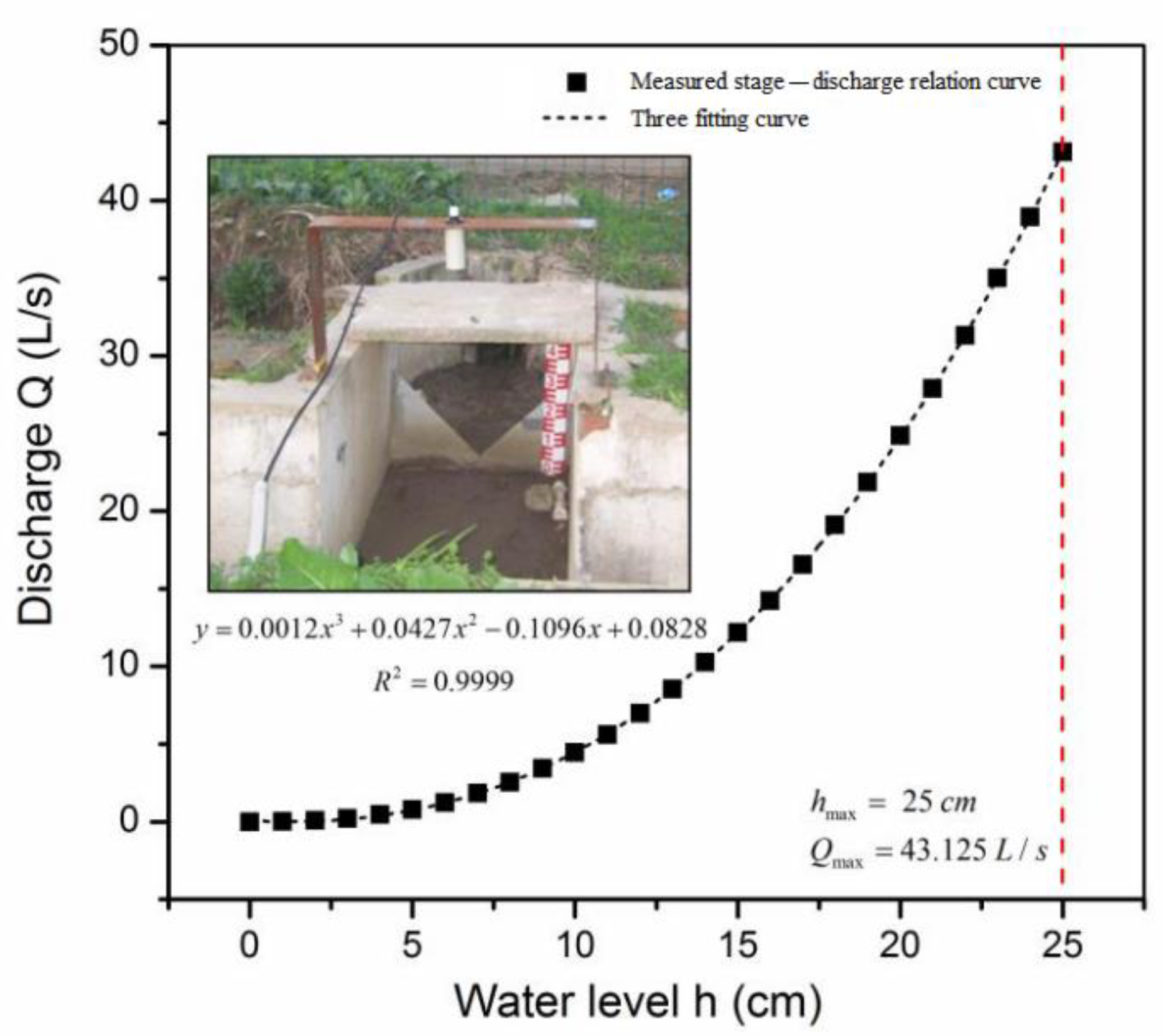
2.1.1. Design of Closed Small Watershed

The field has two drainage ditches built inside and outside with impermeable materials. The outer ditch prevented the exchange of surface water with the surrounding area, while the inner ditch was used to surround the core test area to collect and discharge the surface water generated by runoff and confluence in the study area. Both the inner and outer ditches are trapezoidal in cross-section, with an upper bottom length of 0.7 m and a lower bottom length of 0.4 m, and the average depth is from 0.3–0.4 m. The slope ratio of the ditches is 1:1000 to ensure smooth drainage. A pump was installed at the outlet of the basin to discharge the surface water into the nearby river course automatically.

A meteorological station was installed in the center of the test site to automatically and continuously monitor hydrometeorological elements, such as precipitation, evaporation, temperature, wind speed and wind direction, with a sampling interval of 10 min (Figure 1 and Figure 2a). Precipitation was monitored by a tipping bucket rain gauge, and evaporation was performed using a 255–100 evaporating pan.

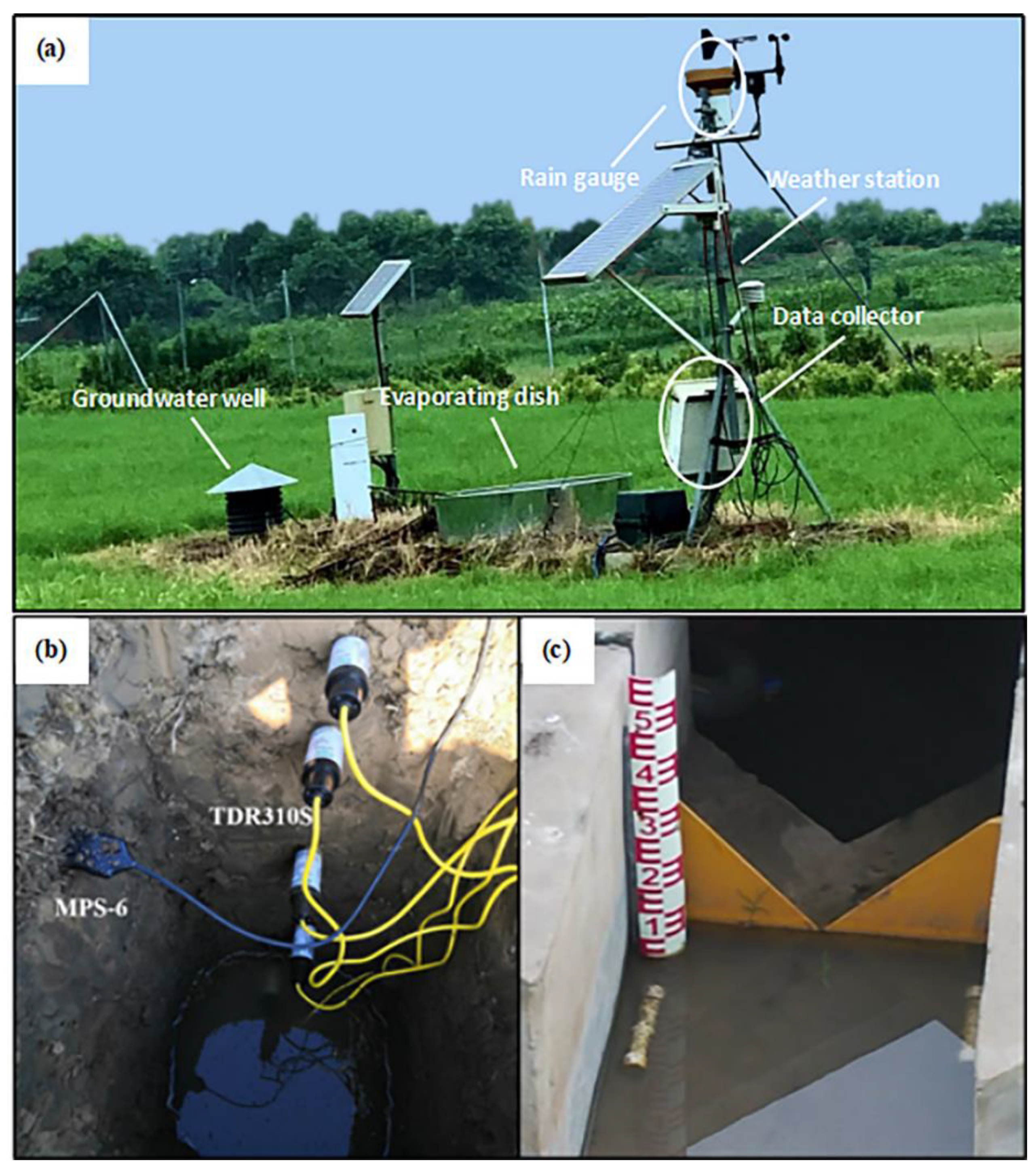
2.1.2. Fine Monitoring of the Whole Process

Soil water content was monitored by the TDR (TDR310S, Acclima, Meridian, ID, USA), which has a three-electrode probe structure, and the measurements are based on the principle of time-domain reflection. That is, the propagation velocity of high-frequency electromagnetic pulse transmission lines in the soil depends on the dielectric properties of the soil, thereby calculating soil water content based on the dielectric constant [44]. Two soil water monitoring profiles were arranged in the BTQ site (Figure 1c), and the TDR probes in each profile were inserted vertically at 10, 20, 40, 60 and 80 cm below the surface, and the sampling time was 10 min (Figure 2b). The soil sensors (MPS-6, Decagon Devices) were buried 10, 20 and 40 cm below the surface in the north and south profiles of the field, and they can automatically monitor soil water potential in a range from −10⁵ to −9 kPa [45].

In the southwest exit of the field, we constructed a concrete channel to drain the water in the ditch to the irrigation ditch outside the experiment field and installed a V-notch weir at the exit (Figure 2c). The water depths in different locations in the ditches were measured with pressure transducers (HOBO Water Level Datalogger, Onset) every 10 min, including in front of the weir, and a certain formula was used to convert it into a flow value (Figure 3). The water level–flow relationship of the V-notch weir was calibrated and verified by the laboratory.

The PVC groundwater wells with a diameter of 0.3 m and a depth of 3 m were installed in the experimental field. The buried depth of groundwater was continuously monitored every 10 min with a laser level meter (JH2004). This observation method is a non-contact measurement technique based on the principle of laser rangefinders. It sends laser pulses to a defined target, measures the time of its regenerate reflection and then converts the buried depth of groundwater according to a certain formula.

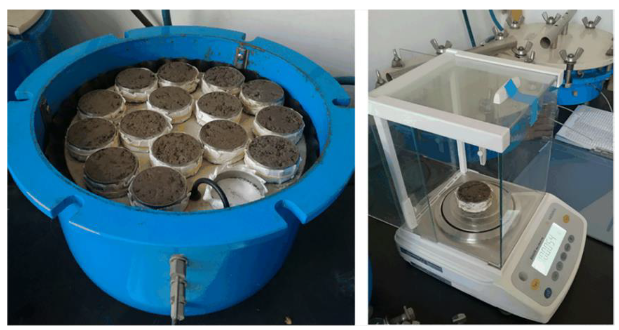
2.1.3. Basic Characteristics of the BTQ Field Soil

The basic characteristics of soil have a certain impact on SWCC [46], and understanding the various basic properties of soils is a necessary step to obtain an accurate and reliable SWCC. Considering the soil formation process of farmland and the influence of human activities, stratification of various properties of soil profiles is common [47]. Some basic properties of soils in the test site were measured and accordingly analyzed in this study.

In this study, the soil from the two profiles in the test field was sampled to analyze the basic soil properties. Samples were taken at depths of 10, 20, 40, 60 and 80 cm below the surface, and each depth was repeated three times. After the soil samples were retrieved, they were spread out in a ventilated area and left to dry naturally for 2–3 days. Impurities were removed, the soil samples were broken up and then sieved through a 2 mm filter to give a uniform texture, and finally, the soil samples were sealed for laboratory testing.

The mechanical components of each horizon of soil were measured using an MS2000 laser for particle sizing analysis [48]. The results show that the silt content of the soil samples ranged from 59.5 to 64.3%, the clay content ranged from 27.4 to 34.9%, and the sand content ranged from 5.6 to 13%. The soil texture of each horizon corresponded to silty clay loam.

The bulk density (γ) of the soil was measured using the core cutter method. The bulk density and organic matter content (OM) of the field had high vertical variability because the field was fallow before renovation. From 2015–2016, the original field was covered with about 30–40 cm of pond sediment. At a depth of 0–20 cm, the value of bulk density showed no significant variation. At a depth of 20–40 cm, the bulk density was the lower of all measured soil horizons, while the organic matter content was the highest, and the soil at this depth corresponds to the topsoil of the original field. The bulk density increased with increasing depth, beginning at a depth of 40–80 cm, while the organic matter content decreased gradually. The result conforms to the vertical distribution law of soil properties of the original cultivated field.

The saturated water content (θ_S) is measured using the oven-drying method [49]. The saturated water content is 0.473 cm³/cm³ at a depth of 0–10 cm (

Table 1. Average and ± standard deviation of the physical and chemical properties and hydraulic parameters of BTQ soil.

Depth (cm)	Clay (%)	Silt (%)	Sand (%)	γ (g/cm3)	OM (g/kg)	θS (cm3/cm3)	Ks (mm/h)
0–10	27.4 (2.18)	59.6 (3.35)	13 (1.14)	1.52 (0.5)	19.5 (2.45)	0.473 (0.02)	1.90 (0.11)
10–20	29.6 (2.06)	64.2 (1.18)	6.2 (2.42)	1.56 (0.08)	8.03 (3.71)	0.401 (0.02)	1.74 (0.13)
20–40	28.3 (1.98)	64.3 (0.83)	7.4 (0.86)	1.43 (0.21)	11.9 (4.21)	0.426 (0.07)	1.36 (0.2)
40–60	31.6 (3.93)	61.0 (1.08)	7.4 (1.69)	1.45 (0.10)	27.7 (4.89)	0.445 (0.05)	0.95 (0.18)
60–80	34.9 (1.08)	59.5 (0.86)	5.6 (0.97)	1.54 (0.09)	24.7 (4.34)	0.434 (0.04)	0.86 (0.08)

), and its value is obviously reduced at a 10–20 cm depth. As the soil porosity increases, the bulk density decreases, the soil relatively loosens and the saturated water content increases. The saturated water content exhibits the greatest variability, as does bulk density, at a depth of 20–40 cm. In the depth range of 40–80 cm, the saturation water content value is relatively stable. In general, the vertical variability of saturated water content in this region shows similar characteristics to the bulk density, indicating that the saturated water content of the soil is closely related to the bulk density.

The saturated hydraulic conductivity (Ks) was measured using the constant-head method [50] based on Darcy’s law of saturation. The cross-sectional area of the core used was 20 cm², the height was 5 mm and the total volume was 100 cm³. The measured values of the saturated hydraulic conductivity of the sampled soil profile decreased with increasing depth, which is inconsistent with the irregular vertical spatial variation of the soil’s physical and chemical properties. This is caused by the uncertainty of the measurement.

2.2. Study Method

2.2.1. The van Genuchten (VG) Model

The VG model was used to fit the SWCC of the laboratory- and field-measured data. The VG model can cover the entire range of the pressure head. Therefore, it is widely used in soil water studies [37]. The VG model is applicable to most soil structures, and only the soil samples with a distinct bimodal pore size distribution do not work well. The soil in this study is silty clay loam, and the VG model has high accuracy in fitting SWCC.

$$\mathsf{\theta }=\{\begin{array}{c}{\mathsf{\theta }}_{\mathrm{r}}+\frac{{\mathsf{\theta }}_{\mathrm{s}}-{\mathsf{\theta }}_{\mathrm{r}}}{{\left[1+{\left(\mathsf{\alpha }\left|\mathrm{h}\right|\right)}^{\mathrm{n}}\right]}^{\mathrm{m}}} ,h<0\\ {\mathsf{\theta }}_{\mathrm{s}} ,h\ge 0\end{array}$$

(1)

where θ (m³/m³) is the soil water content, θ_r and θ_s (m³/m³) are the residual and the saturated soil water contents, respectively, α (kPa⁻¹) is the reciprocal of the intake value, h (cm) is the pressure head, and n characterizes the uniformity of the porous medium.

$$\mathrm{m}=1-\frac{1}{\mathrm{n}}$$

(2)

2.2.2. Numerical Code (HYDRUS-1D)

HYDRUS is a series of software developed by the U.S. Salinity Laboratory in 1991, containing three series: 1D, 2D and 3D [51]. HYDRUS-1D is commonly used to simulate the vertical movement of soil water in unsaturated zones, and Richards equation is used to describe the movement of one-dimensional unsaturated soil water flow; the formula is as follows [52]

$$\frac{\partial \mathsf{\theta }}{\partial \mathrm{t}}=\frac{\partial }{\partial \mathrm{z}}\left[\mathrm{K}\left(\mathrm{h}\right)\left(\frac{\partial \mathrm{h}}{\partial \mathrm{z}}+1\right)\right]-\mathrm{s}\left(\mathrm{z},\mathrm{t}\right)$$

(3)

where t (d) is time, h (cm) is the pressure head, θ (m³/m³) is the soil water content, z (cm) is the vertical space coordinate, K (h) (cm/d) is unsaturated water conductivity and s (z,t) (cm/d) is root-water-uptake rate.

In this study, HYDRUS-1D has applied to inverse the VG model parameters of 0–10, 10–20 and 20–40 cm soil horizons, and the obtained parameters were used to simulate the soil water movement in the BTQ site under precipitation conditions. The upper boundary conditions of the model are set as atmospheric boundary conditions with the surface layer, that is, the precipitation and evaporation data actually monitored in the field. The lower boundary condition chooses a variable pressure head, and the pressure head value is the simulated depth minus the buried depth of groundwater. The initial conditions are set as the soil water content of the profile, and observation points were set at 10, 20 and 40 cm to observe the changes in soil water content in each soil layer.

2.2.3. Numerical Inversion of VG Model Parameters

The VG model parameters based on field monitoring were obtained by numerical inversion of field monitoring data with HYDRUS-1D. The VG model parameters based on laboratory observation were obtained by using the RETention Curve (RETC) inversion of laboratory observation data. The two VG models were compared, analyzed and applied to the simulation of soil water movement under the condition of rainfall infiltration in this region.

The hydrometeorological data monitored in the field from 27 April 2018 to 9 January 2021 were processed. During the study period, 13 precipitation events were screened. The screening criterion was when the total precipitation exceeded 10 mm and the time interval between precipitation events was not less than 24 h. The criterion was used to identify single-peak precipitation events and to reduce the impact of previous precipitation on the process of soil water movement. The 13 precipitation events were divided into two parts, and seven of them were used as input conditions for numerical inversion of the VG model parameters, and the remaining six precipitation events were used to verify the accuracy of obtained VG model in simulating the soil water movement process.

In the laboratory, soil samples were repeated three times in soil layers 10, 20 and 40 cm of two profiles where the TDR was installed. The series of pressures and corresponding soil water content of the collected soil samples were measured by the pressure film meter method (Figure 4). In the laboratory, the soil sample was immersed in water for 24 h to saturation, the total weight of the core and the soil sample was measured with an electronic balance, and then the soil sample was placed on the clay plate in the pressure chamber. The pressure sequence was set to 10, 30, 50, 100, 300, 500 and 1500 kPa, and the soil samples that had reached a steady state under each pressure condition were weighed to calculate the corresponding soil water content. After the soil reached equilibrium at 1500 kPa, the core and the soil sample were placed into an oven and dried until the weight no longer changed, resulting in a sequence of the pressure and the corresponding soil water content. By inputting the soil pressure and the corresponding water content into RETention Curve (RETC), the SWCC of the laboratory was obtained.

Since the SWCC is a highly nonlinear function, the least squares method was used to fit the value of each parameter. The fitting degree was measured by RMSE (root mean square error) and a nonlinear regression correlation index, R,

$$\mathrm{RMSE}=\sqrt{\frac{{\sum }_{\mathrm{i}=1}^{\mathrm{n}}{\left({\mathsf{\theta }}_{\mathrm{i}}-{\mathsf{\theta }}_{\mathrm{i}*}\right)}^2}{\mathrm{n}}}$$

(4)

$$\mathrm{R}=\sqrt{1-\frac{{\sum }_{\mathrm{i}=1}^{\mathrm{n}}{\left({\mathsf{\theta }}_{\mathrm{i}}-{\mathsf{\theta }}_{\mathrm{i}*}\right)}^2}{{\sum }_{\mathrm{i}=1}^{\mathrm{n}}{\left({\mathsf{\theta }}_{\mathrm{i}}-\overline{{\mathsf{\theta }}_{*}}\right)}^2}}$$

(5)

where n is the number of observation points, θ_i and θ_i* are observed and predicted values of the water content, respectively, and θ_* is the arithmetic mean of the water content.

3. Results

3.1. Soil Water Dynamics in the Field

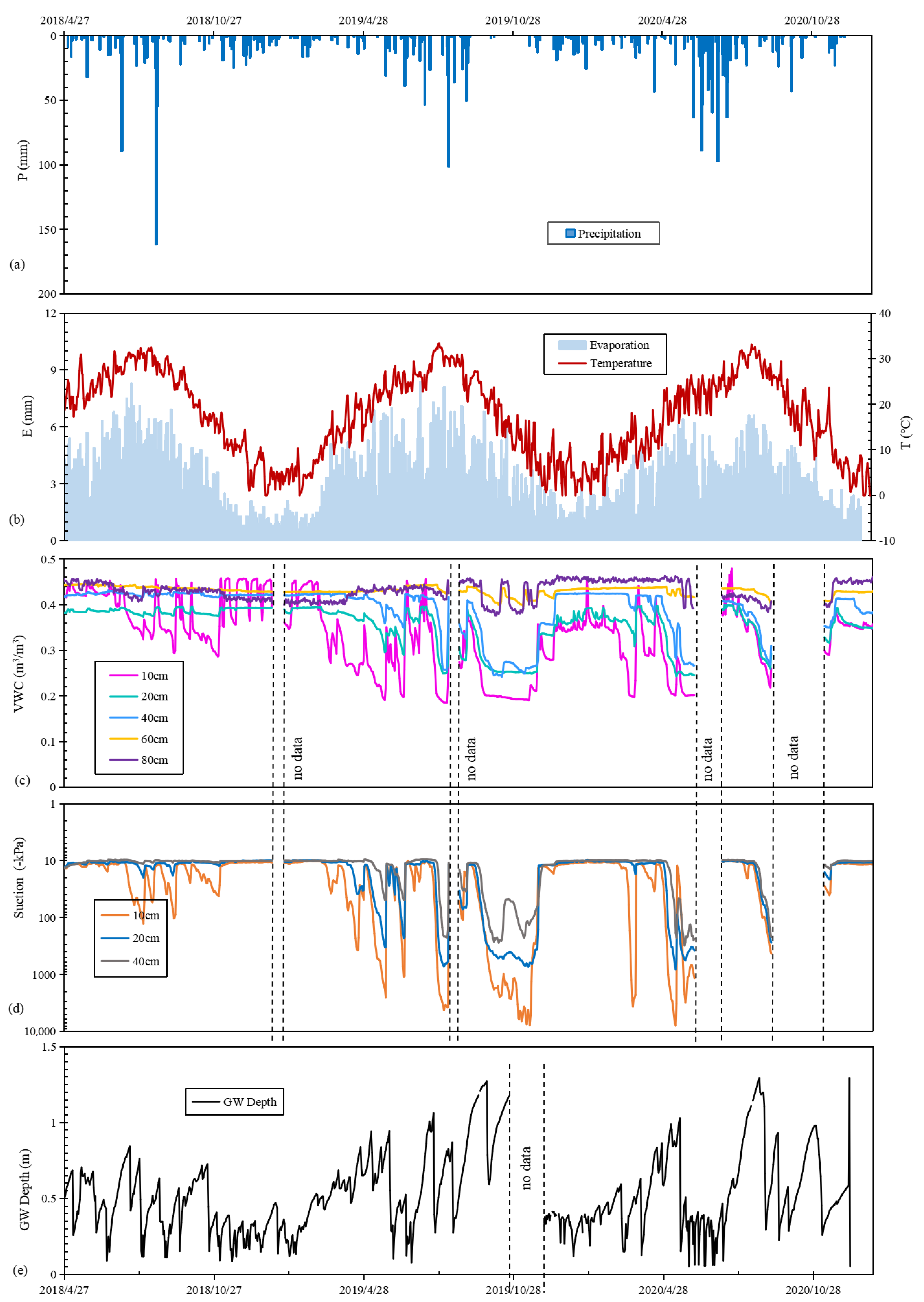
3.1.1. Meteorological and Hydrological Characteristics

The basic meteorological and hydrological characteristics, such as precipitation, evaporation, temperature and groundwater depth, were observed at the BTQ site from 1 April 2018 to 9 January 2021 (Figure 5a,b,e). The groundwater depth from 23 October 2019 to 4 December 2019 was lost due to instrument failure. During the observation period, the total precipitation was 3188 mm, the total evaporation was 2943.9 mm and the average temperature was 23.6 °C.

The maximum daily precipitation was 161.5 mm on 17 August 2018, followed by 101.5 mm on 10 August 2019. It was observed that extreme precipitation events in this region occurred in July or August of each year, which is thought to be caused by typhoons in summer. In general, the precipitation in 2018–2020 is mainly low to moderate precipitation events with less than 25 mm/d. In this region, the temperature is the highest in August of each year, with an average temperature above 30 °C, and the evaporation is also the highest, with a daily average evaporation of over 4.6 mm, while December has the lowest temperature, with an average daily evaporation of less than 1.5 mm. The variation rules of daily average temperature and daily evaporation are basically consistent, and their fluctuations are seasonal, which is related to the seasonal intensity of solar radiation in this region.

The depth of measured groundwater ranged from 0.05 to 1.29 m, and the annual average buried depth was 0.53 m, which is the result of irrigation through artificial channels to control the groundwater level for agricultural production. The measured groundwater dynamics show a rapid response to each heavy precipitation event. With the end of precipitation and continuous evaporation, the groundwater level showed a gradual decrease. For instance, consider the analysis of the precipitation and groundwater level change process from 8:00 on 17 June to 8:00 on 22 June 2019 (Figure 6). Precipitation began at 18:20 on 17 June, but was not intense enough to cause changes in groundwater. When continuous precipitation began at 22:40, the groundwater level began to respond and rapidly rose after 50 min. At 9:10 on 28 June, the groundwater level showed a slight decrease with the cessation of precipitation. When the precipitation ended at 19:40, the groundwater level slowly decreased due to continuous evaporation. At 6:30 on 20 June, the second precipitation event began, and the groundwater level began to rise 70 min later. However, due to the low intensity and discontinuous precipitation, the groundwater level began to decrease slowly after rising to a certain level.

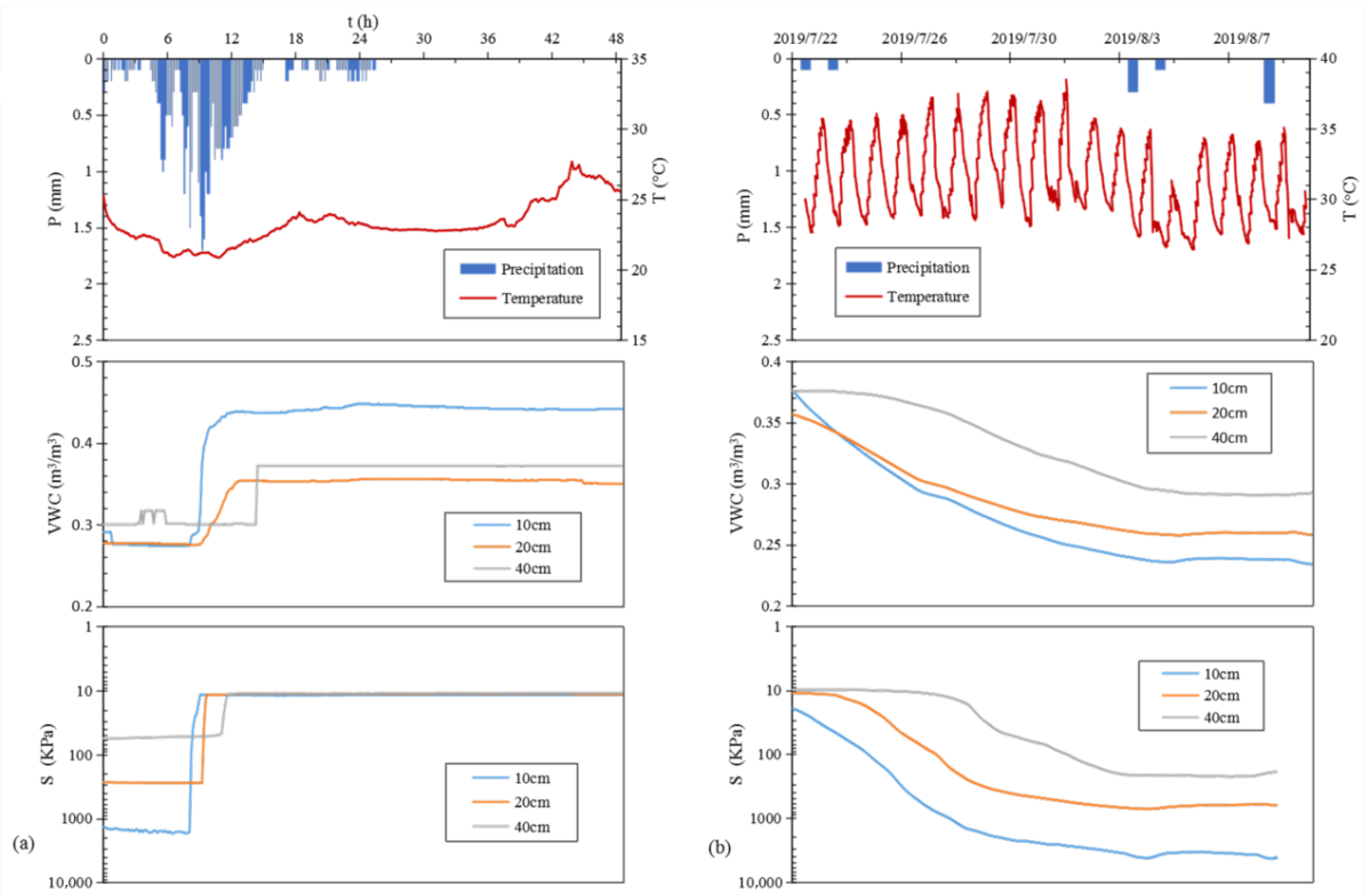
3.1.2. Dynamic Analysis of Soil Water Content and Suction

Soil water content (m³/m³) and suction (-kPa) were monitored at the BTQ site from 26 April 2018 to 9 January 2021 (Figure 5c,d). Due to instrument failure, data were not recorded from 14 January to 20 January 2019 and from 5 June to 8 July 2020. The buried depth of groundwater in BTQ is shallow, so only the unsaturated zone of soil suction at a depth of 0–40 cm below the surface was observed. The water content of the soil horizon at a depth of 0–10 cm ranged between 0.184 and 0.458 m³/m³. The soil water content value range at a 10–20 cm depth is similar to that of a 20–40 cm depth, which is from 0.239–0.400 m³/m³ and 0.236–0.433 m³/m³, respectively. The soil water content ranges from 40–60 and 60–80 cm depth, which is from 0.393–0.447 and 0.369–0.486 m³/m³, respectively.

The minimum measured water content of soil horizons at depths of 0–10, 10–20, 20–40, 40–60 and 60–80 cm was 37, 60, 55, 88 and 79% of the measured maximum, indicating that the soil in this region was basically moist due to the continuous replenishment of shallow groundwater. The soil water content in the depth range of 0–40 cm showed a rapid response to rainfall. Strong precipitation events caused a rapid increase in soil water content. As precipitation ceased and evaporation continued, the water content showed a gradual decrease. The fluctuation of soil water content, whether by precipitation or evaporation, decreases significantly with increasing depth, which is an indication of the gradual weakening of the influence of external conditions on deeper soils. For soil horizons below 40 cm, the soil water content did not respond significantly to precipitation and remained basically stable, except for the abnormal fluctuation from 19 September–9 December 2019. It is presumed that the soil horizon is basically in the saturated or capillary zone above the groundwater surface. Therefore, depths below 40 cm were not considered in the field and laboratory comparisons.

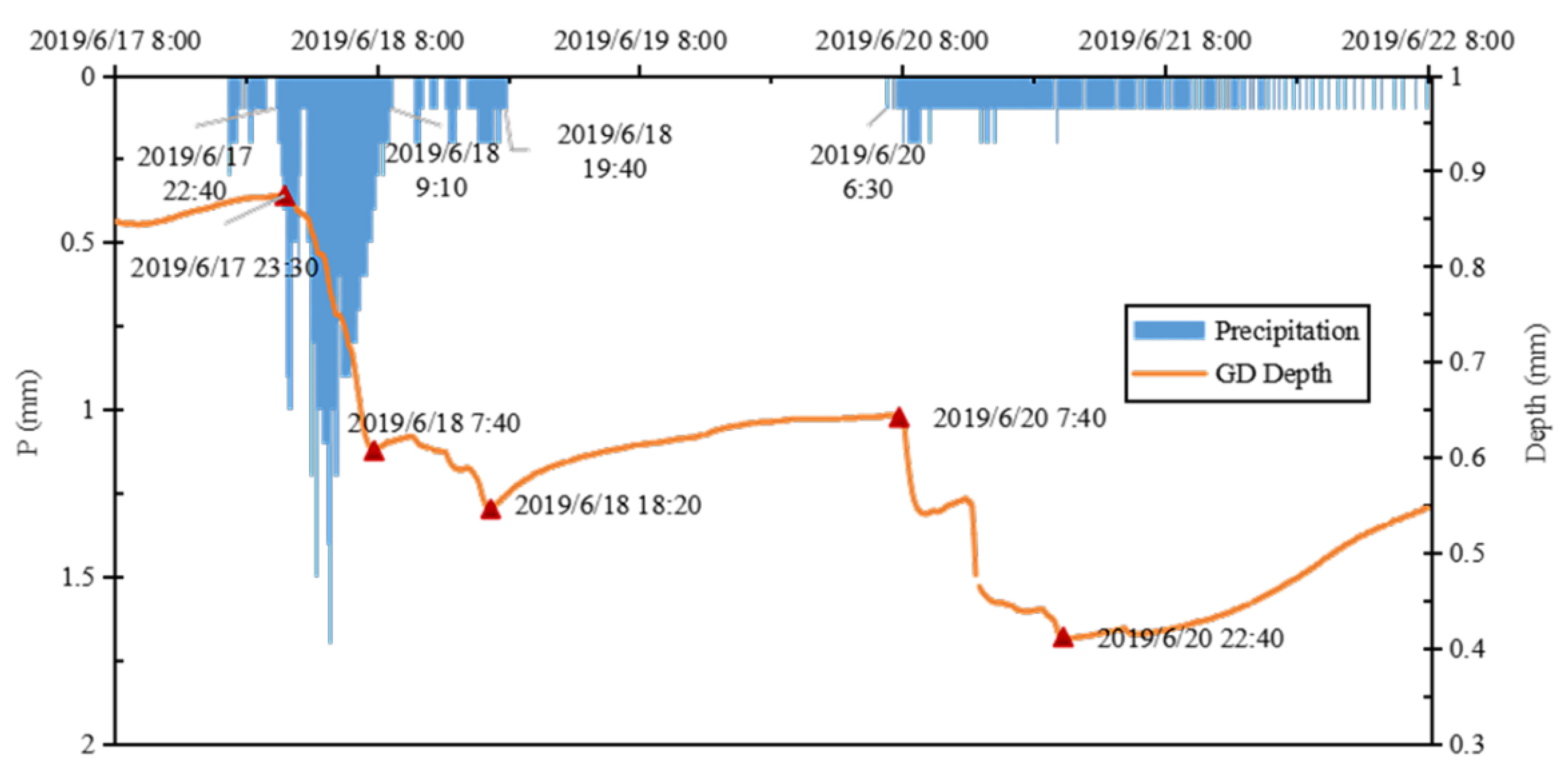
3.1.3. Drying and Wetting Cycle of Soil

During the study period, representative soil wetting and drying processes were analyzed (Figure 7). The typical soil wetting process (Figure 7a) was the precipitation event that started at 18:20 on 17 June 2019, with a total precipitation of 45.9 mm. The soil water content of the 0–40 cm horizon below the surface significantly increased, and the suction also decreased to the lowest recorded value. The response time of soil water content and suction to precipitation became longer with the increasing depth, and at 10–20 cm depth, the trend of soil water content was different from that of suction. Soil suction showed a sharp decrease, while water content slowly increased. In addition, at 20–40 cm depth, the changes in soil water content and suction are not synchronized, where the suction decreased first, and the water content increased about 3 h later. These are all special phenomena caused by rapid infiltration, that is, the change in soil suction or soil water content lag behind on the other side in order to maintain the equilibrium of soil [53]. Even for vertical infiltration at the same point, the changes in soil water content and suction are not identical, which can be obtained by field monitoring. In contrast, the laboratory measurement can only be performed on a single soil sample and cannot understand the response of each soil horizon to a specific vertical infiltration event.

In the process of drying (Figure 7b), the accumulated precipitation was only 2.3 mm, and the temperature fluctuated between 26.4 and 38.5 °C. With constant evaporation, the soil water content and suction of each horizon of soil gradually began to change. The soil water content of each depth of the soil gradually decreased with time, and the soil water content at a depth of 0–10 cm changed from 0.377 to 0.234 m³/m³. At the same time, soil suction gradually increased, and the change was first fast, then slow. From day 11, the change in soil suction was relatively stable. A previous study [54] on evaporation characteristics of soil change over time speculated that the soil water content decreases to a certain value during this period. Soil evaporation is limited by soil moisture, providing only low and stable evaporation and not by evaporation under adequate water supply conditions. Therefore, the consumption of soil water was also relatively low, and the changes in soil water content and suction were relatively flat from the curve. In addition, the variation in soil water content and suction are consistent.

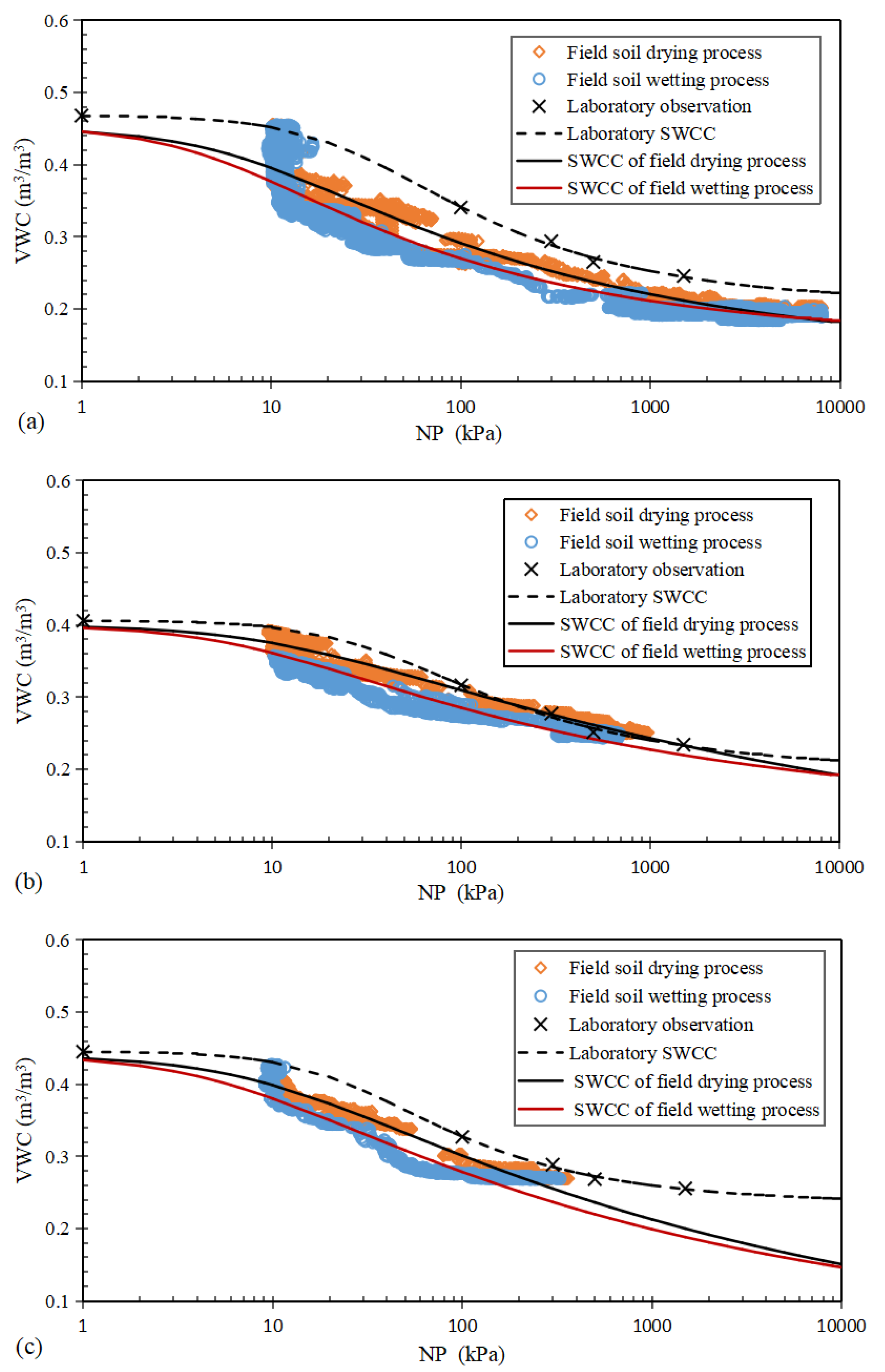
3.2. Results of Parameter Inversion

In the study period, the parameters of the VG model were obtained through numerical inversion of seven precipitation events and ten drying processes in the BTQ site. The actual measured wetting and drying processes in the field were compared with the curves obtained by inversion based on field data and those obtained in the laboratory (Figure 8). The distribution of laboratory measurement points and field observation data is consistent in the soil horizon at 10–20 cm depth because this soil horizon happens to be the compacted horizon of the overlying soil, with high bulk density and relatively uniform pore distribution. However, the laboratory measurement points out that the 0–10 and 20–40 cm horizons did not overlap with the field observation points. In general, it can be seen that the soil water content measured in the laboratory is higher than that observed in the field under the same water-wetting condition. On the one hand, the two horizons of soil were the current and the original topsoil horizon with relatively complex and heterogeneous soil pore structures. On the other hand, the soil samples observed in the laboratory were subjected to vibration during collection and transportation, and the soil structure was changed to some extent.

The saturated water content is the water content of the soil when all the pores are filled with water. When analyzing the soil water content measured in the field, the maximum water content was considered as the saturated water content. The saturated soil water content (θ_s) measured in the field was 0.458, 0.400 and 0.433 m³/m³ at 0–10, 10–20 and 20–40 cm depths, respectively. The saturated water content of each soil horizon obtained from the inversion of parameters based on field wetting processes was 0.454, 0.400 and 0.441 m³/m³ and the θ_s obtained from the drying processes were 0.451, 0.400 and 0.440 m³/m³. The residual soil water content values obtained in the laboratory for each soil horizon were 0.207, 0.196 and 0.232 m³/m³, and those obtained based on the wetting and drying processes in the field were 0.158, 0.135, 0.048 m³/m³ and 0.134, 0.046, 0.016 m³/m³, respectively (

Table 2. Field and laboratory parameter inversion results and fitness index.

	Depth (cm)	θr (m3/m3)	θs (m3/m3)	α (kPa−1)	n	RMSE (m3/m3)	R2
Silty clay loam (reference) [55]		0.089	0.43	0.19	1.23
Field soil wetting	0–10	0.158	0.454	0.19	1.32	0.014	0.842
	10–20	0.135	0.400	0.13	1.21	0.009	0.847
	20–40	0.048	0.441	0.11	1.18	0.013	0.787
Field soil drying	0–10	0.134	0.451	0.14	1.26	0.014	0.949
	10–20	0.046	0.400	0.09	1.13	0.012	0.937
	20–40	0.016	0.440	0.10	1.16	0.010	0.807
Laboratory observation	0–10	0.207	0.468	0.04	1.49	-	-
	10–20	0.196	0.406	0.03	1.47	-	-
	20–40	0.232	0.445	0.04	1.58	-	-

).

The results for the reciprocal of the intake values (α) based on field data were 0.19, 0.13, 0.11 for wetting and 0.14, 0.09, 0.1 kPa⁻¹ for drying, while the values obtained in the laboratory were 0.04, 0.03 and 0.04 kPa⁻¹. The values of the uniformity of porous medium (n) based on field data were 1.32, 1.21, 1.18 and 1.26, 1.13, 1.16, and the values obtained in the laboratory were 1.49, 1.47, and 1.58.

In addition, the inversion of parameters based on field-monitored soil wetting and drying processes showed RMSEs (root mean square error) of 0.014, 0.009, 0.013 and 0.014, 0.012, 0.010 m³/m³ for 0–10, 10–20, and 20–40 cm depths, with R correlation indices of 0.842, 0.847, 0.787 and 0.949, 0.937, 0.807, respectively.

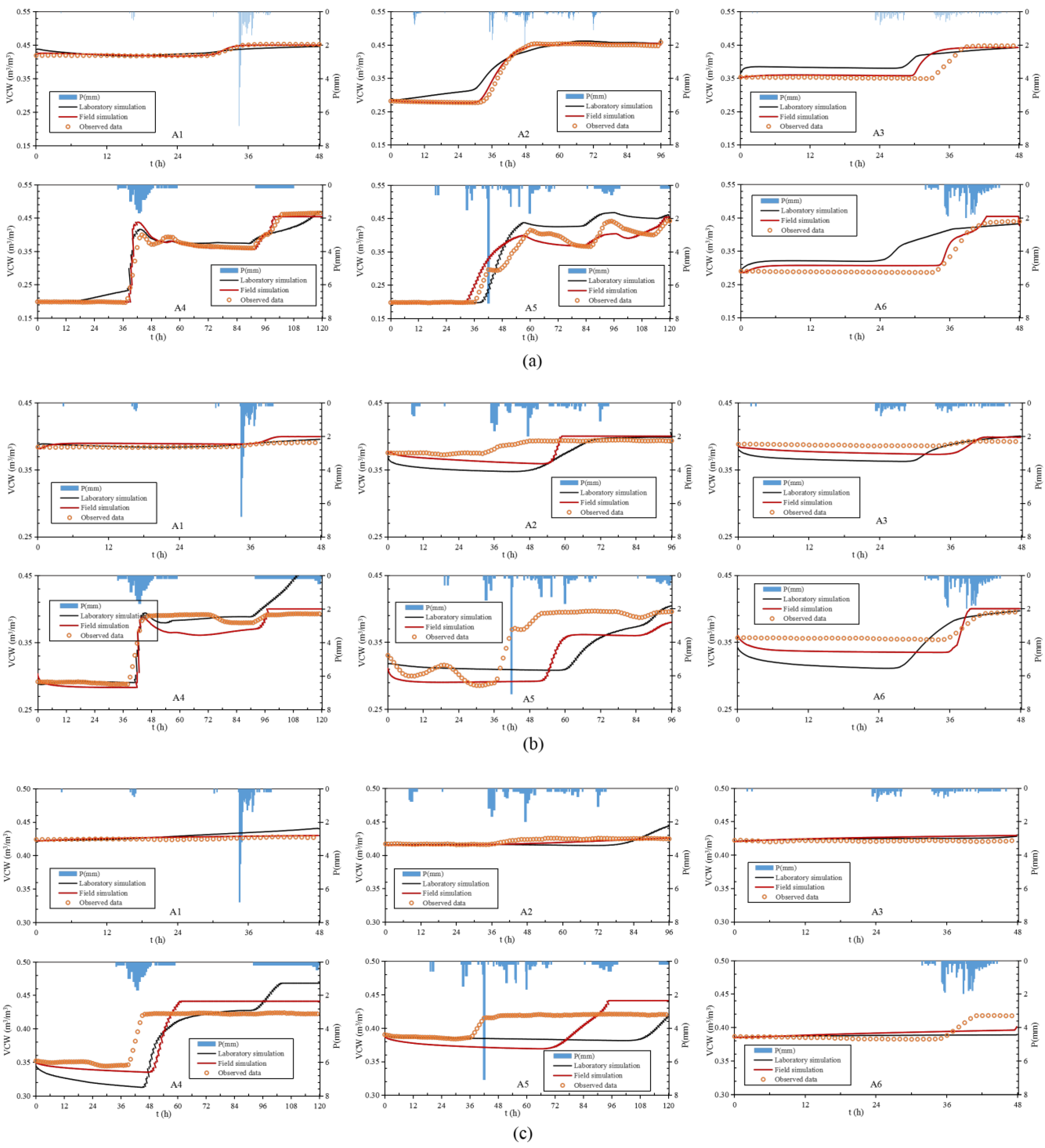
3.3. Soil Water Dynamic Simulation

Rainfall causes floods in the watershed of the study area, and it is of great significance to analyze the variation of soil water under rainfall conditions in the region. Soil water movement was simulated for the remaining six precipitation events, A1, A2, A3, A4, A5 and A6, during the study period using the SWCC obtained from the field-wetting process and laboratory, as shown in Figure 9. The characteristics of the six precipitation events (

Table 3. Characteristics of precipitation events recorded at field sites in BTQ.

Event Code	Start Time	P mm	T h	I mm h−1	PMAX mm h−1
A1	2018/05/24 8:00	28.7	48	0.598	16.0
A2	2018/11/05 8:00	36.4	96	0.379	4.5
A3	2018/11/16 8:00	18.8	48	0.392	2.4
A4	2019/06/17 8:00	64.0	120	0.533	7.1
A5	2020/03/24 8:00	49.7	120	0.414	8.0
A6	2020/04/18 8:00	35.2	48	0.733	8.3

Cumulative precipitation, P (mm); duration of rainfall, T (h); average rain intensity, I (mm h⁻¹); maximum rain intensity, PMAX (mm h⁻¹).

) showed that they were mainly moderate precipitation events, which were consistent with the precipitation characteristics of the plains of the Taihu Basin.

Soil water movement simulations for the six precipitation events were observed (Figure 9) and compared with actual field monitoring. (Figure 9, Table 3 and

Table 4. Fitting index of soil water dynamic simulation.

Event Code	P (mm)	10 cm		20 cm		40 cm
		Field (Laboratory)		Field (Laboratory)		Field (Laboratory)
		RMSE (m3/m3)	R	RMSE (m3/m3)	R	RMSE (m3/m3)	R
A1	28.7	0.003 (0.006)	0.983 (0.898)	0.005 (0.002)	0.89 (0.924)	0.002 (0.005)	0.714 (0.838)
A2	36.4	0.007 (0.026)	0.997 (0.980)	0.017 (0.027)	0.639 (0.705)	0.004 (0.006)	0.833 (0.299)
A3	18.8	0.017 (0.027)	0.889 (0.869)	0.008 (0.014)	0.927 (0.882)	0.004 (0.003)	0.050 (0.077)
A4	64	0.017 (0.020)	0.985 (0.823)	0.017 (0.008)	0.959 (0.927)	0.027 (0.038)	0.842 (0.848)
A5	49.7	0.029 (0.029)	0.962 (0.981)	0.045 (0.048)	0.789 (0.654)	0.033 (0.023)	0.468 (0.043)
A6	35.2	0.015 (0.042)	0.990 (0.808)	0.014 (0.020)	0.981 (0.882)	0.009 (0.010)	0.62 (0.505)
Mean		0.015 (0.025)	0.968 (0.895)	0.018 (0.020)	0.864 (0.819)	0.013 (0.014)	0.588 (0.435)

). The total precipitation for A1 was 28.7 mm, and the maximum rain intensity was 16 mm/h. The precipitation was concentrated at 18:00 on 25 May. In this precipitation event, the soil was relatively wet at the beginning and became saturated soon after the precipitation started. The RMSE of the simulated soil water movement process from the VG model obtained, based on field monitoring data, were 0.003, 0.005 and 0.002 m³/m³, and R was 0.983, 0.89 and 0.714, respectively. The total precipitation of A2 was 36.4 mm, but the precipitation duration was long, with a maximum of 4.5 mm/h. The soil gradually became saturated from dryness. In this case, the fitted R of the three soil layers based on field monitoring data were 0.007, 0.017 and 0.004, while the R was 0.026, 0.027 and 0.006, respectively, based on the laboratory analysis. A3 and A2 had similar characteristics, but A3 soil was relatively wet before the onset of precipitation, with little change in soil water content, especially in deeper soil. The field monitoring instrument showed slight fluctuations within the allowable error range, while the curve of deep soil moisture content was relatively flat and did not fluctuate during the simulation. Therefore, the simulation was good in other soil layers, but the correlation of soil moisture movement simulation in the 20–40 cm soil layer was poor, with a value of 0.05. The total precipitation in A4 was 64 mm, and the precipitation was concentrated in the early stage. The decrease in groundwater depth makes the deep soil saturate quickly, while the surface soil is gradually saturated in the later precipitation process. The VG model parameters obtained based on field data can simulate the actual situation. The precipitation of A6 was relatively concentrated, and the rain intensity was strong. The soil responded quickly after the precipitation started. The field simulation results for each horizon of soil in A6 showed the field data simulations RMSE of 0.015, 0.014, and 0.009 m³/m³, compared with laboratory-based RMSE of 0.042, 0.02 and 0.01 m³/m³, respectively.

A5 occurred from 8:00 on 24 March to 8:00 on 29 March 2020, with a total precipitation of 49.7 mm. In this precipitation event, there were two precipitation processes, and the time interval was less than 24 h, so it was classified as a precipitation event. The first precipitation ended at 8:00 on 27 March, but the soil did not reach saturation. With the end of precipitation and continuation of evaporation, the surface soil water content gradually decreased, but due to the short time interval considered, the parameters of deep soil did not change significantly. At 20:00 on the 27th, the second precipitation started, and the soil water content increased accordingly. This complex process of initial surface wetting, drying and finally wetting causes difficulty for the simulation. Due to the limitations of the model, the whole process cannot be adequately represented, so the simulation results were not satisfactory.

The mean RMSE (Table 4) of 0–10, 10–20 and 20–40 cm soil horizons fitted in the field were 0.015, 0.018 and 0.013 m³/m³, all less than 0.02. For the correlation index R (Table 4), the values were 0.968 and 0.864 at a depth of 0–10 and 10–20 cm, which were greater than 0.8. However, at a depth of 20–40 cm, the fit was not satisfactory, with a value of 0.588. The results of simulated soil water movement based on laboratory data showed that the average RMSE for each soil horizon was 0.025, 0.020 and 0.014 m³/m³, and the R was 0.895, 0.819 and 0.435, respectively.

4. Discussion

4.1. Influencing Factors of Soil Water Movement

Through the analysis of six simulated precipitation events, it is found that rainfall is the main source of soil moisture change in this region. Among them, the soil water content of A4 changed the most after precipitation, and the soil water content at 10, 20 and 40 cm depth increased by 0.269, 0.105 and 0.080 m³/m³, respectively. A1 showed the smallest change in soil water content, with an increase of 0.035, 0.007 and 0.004 m³/m³ at 10, 20 and 40 cm depths. The varying degree of soil water content under each precipitation event is in the order of A4 > A5 > A6 > A2 > A3 > A1, while the total precipitation is in the order of A4 > A5 > A2 > A6 > A1 > A3. The difference between the total precipitation of A6 and A2 is 1.2 mm, but the precipitation duration of A2 is comparatively longer, and the total evaporation is 6 mm, which is 3 mm higher than that of A6. Therefore, the change in soil water content is not as great as that of A6. The variation in soil water content in A1 is lower than in A3 because A1 occurs in summer with a total evaporation of 10.3 mm, while A3 occurs in winter with a total evaporation of 3 mm. During precipitation, the greater the evaporation, the smaller the change in soil water content.

From the above analysis, it can be seen that precipitation is the main factor of soil water movement, evaporation also has a certain impact on the change of soil water content, and the movement of water in the topsoil is comparatively more violent; the deeper the soil, the smaller the change in water content. Zhou et al. [56] found that changes in soil water content are affected by precipitation, vegetation types, soil evaporation and other factors. Wang et al. [57] found that different texture configurations of soil had certain effects on water movement and solute transport according to experiments. The soil texture in this region is silty clay loam. In the future, we will consider establishing field test sites in different regions to explore the influence of different soil textures on soil water movement

Soil texture, precipitation and evaporation are the main factors affecting soil water movement [58], which helps to understand better the rules of soil water movement and the process of runoff in humid plain areas with similar characteristics.

4.2. Accuracy of VG Model Parameter Inversion

Some researchers proposed an improved VG model for clayey soils. Compared with the BC model [35,36], the VG model has a higher fitting accuracy for the SWCC of sandy and silt loams [39]. VG model parameters are the basis for understanding and accurately simulating soil water movement and the key to improving the simulation accuracy [59]. Based on the soil characteristics in the study area, the VG model was finally selected for the dynamic simulation of soil water. The VG model parameters obtained from the field wetting and drying process data were compared and analyzed with those obtained from the laboratory, and the differences were evident for all the soil horizons.

The saturated soil water content (θ_s) measured in the field was 0.458, 0.400 and 0.433 m³/m³ at 0–10, 10–20 and 20–40 cm depths, respectively. The values of θ_s obtained from the wetting and drying processes were closer to the actual monitoring values. However, the θ_s of each horizon of soil obtained in the laboratory is relatively large because the soil becomes dry during sampling and transport, resulting in a decrease in soil viscosity. Residual water content [60] (θ_r) refers to the soil water content decreasing to a critical value, and the soil water content will not decrease when the suction continues higher. The minimum water contents at depths of 0–10, 10–20 cm and 20–40 cm in this area are 0.184, 0.239 and 0.236 m³/m³, respectively. By definition, θ_r should be less than the minimum soil moisture content. Therefore, it can be concluded that the value of θ_r for the 0–10 cm soil horizon obtained in the laboratory is unreasonable. In addition, the reference value of θ_r in the VG model for silty clay loam is 0.089 [55], which shows that the results obtained from field observations are more consistent with the soil types in this area. For the parameters α and n, there is a large gap between the parameter values obtained by laboratory data and those obtained by field data. By comparing the results, it is concluded that the parameters α and n obtained by field data are generally closer to the corresponding parameter reference values of 0.19 and 1.23 for silty clay loam [55] in the region.

In the field data, the RMSE of soil wetting and drying processes at 0–10, 10–20 and 20–40 cm depths were all lower than 0.015 m³/m³, and the correlation indices, R, were all higher than 0.787. The statistical results indicated that the inversion parameters of the field observed data were comparatively better. Liyama [53] and Sorbino et al. [61] found that the θ measured in the field were often about 10% smaller than those in the laboratory. This suggests that it is difficult to restore the actual SWCC in the field only by laboratory observation data. In addition, the practicability of SWCC based on field observation in soil water movement simulation needs to be further evaluated and validated.

4.3. Application of Soil–Water Characteristic Curve

In order to verify the reliability and accuracy of the SWCC, the precipitation event was simulated by HYDRUS-1D with the measured precipitation, evaporation and groundwater level as the input conditions of the model. The soil water movement simulated based on field data was compared and analyzed with the laboratory simulation results.

The average RMSE of 10, 20 and 40 cm horizons of soil water movement simulated by SWCC based on field monitoring data were 0.0150, 018 and 0.013 m³/m³ (all less than 0.02 m³/m³), with R values of 0.968, 0.864 and 0.588, respectively. All of the fit indexes were better than the laboratory (Figure 9). The error of this study is close to that of Wu et al. [62], who simulated the soil water movement in the black soil area of Northeast China, wherein they obtained a simulation error within ± 10%. Wang et al. [63] also confirmed that HYDRUS-1D could accurately describe water movement in stratified soil; their RMSE for calibration and validation ranged from 3.2 to 10% and from 2.5 to 13.6%, respectively.

In summary, it is believed that the simulation based on field data can reproduce the water movement and change process more accurately, which is consistent with the law of precipitation infiltration in the plain area and provides a reliable theoretical basis for the calculation of soil movement and runoff production in the plain area.

In addition, it is necessary to consider further the impact of hysteresis in the water balance process [64] and increase the simulation of soil runoff and flow in the field [65] so as to improve further the simulation accuracy and the calculation results of the model and obtain an SWCC suitable for the plain area of the Taihu Basin.

5. Conclusions

In this study, a small-scale field experiment of soil water movement in an unsaturated zone was carried out at the BTQ experimental base in the Taihu Basin. The data of precipitation, evaporation, soil water content, soil suction and groundwater depth were continuously monitored every ten minutes to explore the characteristics of soil water variation in the field, and the SWCC was constructed and compared with the curve obtained using common laboratory methods. The process of soil water movement in the unsaturated zone under the condition of precipitation was simulated to explore the mechanisms of soil water movement in the unsaturated zone of the Taihu Basin. The key findings are summarized below.

Through the analysis of the collected soil physical and chemical properties and hydrometeorological data, the results showed that the soil in the test area is silty clay loam, and the soil moisture frequently varied from April to September each year but remained stable from October to March. The extent of soil wetting and drying due to external conditions decreases with depth, and the soil horizon above 40 cm in depth is basically in the saturated zone, or the capillary zone when just below this depth. Soil water changes most frequently and severely in the soil horizon at 0–40 cm depth below the surface. The soil water content and suction in the field were analyzed, and the characteristics of soil water variation in this region were summarized by describing the typical dry–wet soil processes.

The values of soil hydraulic characteristic parameters obtained from the inversion of field data are quite different from those measured in the laboratory. Compared with those measured in the laboratory, the field-measured curves in each depth range are more consistent with the characteristics of silty clay loam and the real situation in the field.

The precipitation events were simulated by using the parameters obtained from the inversion of the wetting process data measured in the field and the results measured in the laboratory. The RMSE of 0–10, 10–20 and 20–40 soil horizon simulations are 0. 015, 0.018 and 0.014 m³/m³, respectively. In all the horizons of soil, the simulation results based on the field data showed significantly better correspondence than the results of the laboratory simulation and were more consistent with the changes in soil water content measured in the field.

This research method is feasible for small-scale experimental areas, and some scholars suggest that it is meaningful to extend the discovered mechanism to small- to catchment-scale [66]. Therefore, the soil hydraulic characteristic parameters of this experimental base can be referred to when studying other humid plain areas. In humid plains, the vegetation is abundant, and root water wetting and leaf transpiration have a certain influence on soil water movement, which will be considered in further study. In addition, the observation of surface runoff data should be added to simulate the hydrological process of the BTQ experimental field and reflect the hydrological cycle characteristics and runoff generation mechanisms of the humid plain areas.

References

1. Smith, A.; Tetzlaff, D.; Gelbrecht, J.; Kleine, L.; Soulsby, C. Riparian wetland rehabilitation and beaver re-colonization impacts on hydrological processes and water quality in a lowland agricultural catchment. Sci. Total Env. 2020, 699, 134302. [Google Scholar] [CrossRef] [PubMed]
2. Yu, L.; Rozemeijer, J.; van Breukelen, B.M.; Ouboter, M.; van der Vlugt, C.; Broers, H.P. Groundwater impacts on surface water quality and nutrient loads in lowland polder catchments: Monitoring the greater Amsterdam area. Hydrol. Earth Syst. Sci. 2018, 22, 487–508. [Google Scholar] [CrossRef] [Green Version]
3. Glavan, M.; Cvejic, R.; Tratnik, M.; Pintar, M. Geospatial Analysis of Water Resources for Sustainable Agricultural Water Use in Slovenia. In Current Perspectives in Contaminant Hydrology and Water Resources Sustainability; InTech: Rijeka, Croatia, 2013; pp. 199–219. [Google Scholar]
4. De Carlo, L.; Perkins, K.; Caputo, M.C. Evidence of Preferential Flow Activation in the Vadose Zone via Geophysical Monitoring. Sensors 2021, 21, 1358. [Google Scholar] [CrossRef]
5. Doudill, A.J.; Heathwaite, A.L.; homas, D.S.G.T. Soil water movement and nutrient cycling in semi-arid rangeland_ vegetation change and system resilience. Hydrol. Process. 1998, 12, 443–459. [Google Scholar]
6. Pu, H.; Song, W.; Wu, J. Using Soil Water Stable Isotopes to Investigate Soil Water Movement in a Water Conservation Forest in Hani Terrace. Water 2020, 12, 3520. [Google Scholar] [CrossRef]
7. Touma, J.; Vachaud, G. Air and water flow in a sealed, ponded vertical soil column experiment and model. Soil Sci. 1984, 137, 181–187. [Google Scholar] [CrossRef]
8. Wang, Z.; Feyen, J.; Nielsen, D.R.; van Genuchten, M.T. Two-phase flow infiltration equations accounting for air entrapment effects. Water Resour. Res. 1997, 33, 2759–2767. [Google Scholar] [CrossRef]
9. Han, D.; Zhou, T. Soil water movement in the unsaturated zone of an inland arid region: Mulched drip irrigation experiment. J. Hydrol. 2018, 559, 13–29. [Google Scholar] [CrossRef]
10. Zhao, T.; Zhu, Y.; Wu, J.; Ye, M.; Mao, W.; Yang, J. Quantitative Estimation of Soil-Ground Water Storage Utilization during the Crop Growing Season in Arid Regions with Shallow Water Table Depth. Water 2020, 12, 3351. [Google Scholar] [CrossRef]
11. Kumar, C.P.; Seth, S.M. Derivation of Soil Moisture Retention Characteristics from Saturated Hydraulic Conductivity. Natl. Inst. Hydrol. 2001, 49, 653–657. [Google Scholar]
12. Xiang, J.; Xu, Y.; Yuan, J.; Wang, Q.; Wang, J.; Deng, X. Multifractal Analysis of River Networks in an Urban Catchment on the Taihu Plain, China. Water 2019, 11, 2283. [Google Scholar] [CrossRef] [Green Version]
13. Uhlenbrook, S. Catchment hydrology—A science in which all processes are preferential. Hydrol. Process. 2006, 20, 3581–3585. [Google Scholar] [CrossRef]
14. De Carlo, L.; Battilani, A.; Solimando, D.; Caputo, M.C. Application of time-lapse ERT to determine the impact of using brackish wastewater for maize irrigation. J. Hydrol. 2020, 582, 124465. [Google Scholar] [CrossRef]
15. Kalbus, E.; Reinstorf, F.; Schirmer, M. Measuring methods for groundwater–surface water interactions. Hydrol. Earth Syst. Sci. 2006, 10, 873–887. [Google Scholar] [CrossRef] [Green Version]
16. Sophocleous, M. Interactions between groundwater and surface water: The state of the science. Hydrogeol. J. 2002, 10, 52–67. [Google Scholar] [CrossRef]
17. Winter, T.C. Recent advances in understanding the interaction of groundwater and surface water. Rev. Geophys. 1995, 33, 985–994. [Google Scholar] [CrossRef]
18. Fredlund, D.G.; Xing, A. Equations for the soil-water characteristic curve. Can. Geotech J. 1994, 31, 521–532. [Google Scholar] [CrossRef]
19. Habasimbi, P.; Nishimura, T. Soil Water Characteristic Curve of an Unsaturated Soil under Low Matric Suction Ranges and Different Stress Conditions. Int. J. Geosci. 2019, 10, 39–56. [Google Scholar] [CrossRef] [Green Version]
20. Huyakorn, P.S.; Thomas, S.D. Techniques for Making Finite Elements Competitve in Modeling Flow. Water Resour. Res. 1984, 20, 1099–1135. [Google Scholar] [CrossRef]
21. Jordan, P. Hillslope hydrology and stability. Can. Water Resour. J./Rev. Can. Des Ressour. Hydr. 2014, 40, 126–127. [Google Scholar] [CrossRef]
22. Wosten, J.H.M.; Genuchten, M.T.V. Using Texture and Other Soil Properties to Predict the Unsaturated Soil Hydraulic Functions. Soil Sci. Am. J. 1988, 52, 1762–1770. [Google Scholar] [CrossRef]
23. Heshmati, A.A.; Motahari, M.R. Identification of key parameters on soil water characteristic curve. Life Sci. J. 2012, 9, 1532–1537. [Google Scholar]
24. Cresswell, H.P.; Green, T.W.; McKenzie, N.J. The Adequacy of Pressure Plate Apparatus for Determining Soil Water Retention. Soil Sci. Soc. Am. J. 2008, 72, 41–49. [Google Scholar] [CrossRef]
25. Bittelli, M.; Flury, M. Errors in Water Retention Curves Determined with Pressure Plates. Soil Sci. Soc. Am. J. 2009, 73, 1453–1460. [Google Scholar] [CrossRef] [Green Version]
26. McQUEEN, I.S.; Miller, R.F. Calibration and evalution of a wide-range gravimetricmethod for measuring mois. Soil Sci. 1968, 106, 225–231. [Google Scholar] [CrossRef]
27. Bordoni, M.; Bittelli, M.; Valentino, R.; Chersich, S.; Meisina, C. Improving the estimation of complete field soil water characteristic curves through field monitoring data. J. Hydrol. 2017, 552, 283–305. [Google Scholar] [CrossRef]
28. Zhao, Y.; Wang, W.; Wang, Z.; Li, L.C. Physico-empirical methods for estimating soil water characteristic curve under different particle size. In Proceedings of the IOP Conference Series: Earth and Environmental Science, Kaohsiung City, Taiwan, 17–21 July 2018; p. 012018. [Google Scholar]
29. Gupta, S.C.; Larson, W.E. Estimating Soil Water Retention Characteristics From Particle Size. Water Resour. Res. 1979, 15, 1633–1635. [Google Scholar] [CrossRef]
30. Vereecken, H.; Maes, J.; Feyen, J.; Darius, P. Estimating the Soil Moisture Retention Characteristic from Texture, Bulk Density, and Carbon Content. Soil Sci. 1989, 148, 389–403. [Google Scholar] [CrossRef]
31. Schaap, M.G.; Leij, F.J.; Genuchten, M.T.v. Neural Network Analysis for Hierarchical Prediction of Soil Hydraulic Properties. Soil Sci. Am. J. 1998, 62, 847–855. [Google Scholar] [CrossRef]
32. Lalit, M.; Arya, L.F.J.; Genuchten, M.T.v.; Shouse, P.J. Scaling Parameter to Predict the Soil Water Characteristic from Particle Size Distribution Data. Soil Sci. Am. J. 1999, 63, 510–519. [Google Scholar]
33. Tyler, S.W.; Wheatcraft, S.W. Fractal Processes in Soil Water Retention. Water Resour. Res. 1990, 26, 1047–1054. [Google Scholar] [CrossRef]
34. Liu, J.; Xu, S.; LIU, H. A review of development in estimating soil water retention characteristics from soil data. J. Hydraul. Eng. 2004, 2, 68–76. [Google Scholar]
35. Brooks, R.H.; Corey, A.T. Hydraulic properties of porous media and their relation to drainage design. Trans. ASAE 1964, 7, 26–28. [Google Scholar]
36. Brooks, R.H.; Corey, A.T. Properties of porous media affecting fluid flow. J. Irrig. Drain. Eng. 1966, 92, 61–88. [Google Scholar] [CrossRef]
37. Van Genuchten, M.T. A Closed-form Equation for Predicting the Hydraulic Conductivity of Unsaturated Soils. Soil Sci. Soc. Am. J. 1980, 44, 892–898. [Google Scholar] [CrossRef] [Green Version]
38. Gardner, W.R. Some steady-state solutions of the unsaturated moistureflow equation with application to evaporation from a water table. US Dcpariment Agric. 1957, 85, 228–232. [Google Scholar]
39. Russo, D. Determining Soil Hydraulic Properties by Parameter Estimation. Water Resour. Res. 1988, 24, 453–459. [Google Scholar] [CrossRef]
40. Whisler, F.D.; Watson, K.K. One-dimensional gravity drainage of uniform columns of porous materials. J. Hydrol. 1968, 6, 277–296. [Google Scholar] [CrossRef]
41. Zachmann, D.W.; Chateau, P.C.D.; Klute, A. Simultaneous approximation of water capacity and soil hydraulic conductivity by parameter identification. Soil Sci. 1982, 134, 0038–0075X. [Google Scholar] [CrossRef]
42. Šimůnek, J.; van Genuchten, M.T. Estimating Unsaturated Soil Hydraulic Properties from Tension Disc Infiltrometer Data by Numerical Inversion. Water Resour. Res. 1996, 32, 2683–2696. [Google Scholar] [CrossRef]
43. Dane, J.H.; Hruska, S. In-Situ Determination of Soil Hydraulic Properties during Drainage. Soil Sci. Soc. Am. J. 1983, 47, 619–624. [Google Scholar] [CrossRef]
44. Topp, G.C.; Davis, J.L.; Annan, A.P. Electromagnetic determination of soil water content: Measurements in coaxial transmission lines. Water Resour. Res. 1980, 16, 574–582. [Google Scholar] [CrossRef] [Green Version]
45. Nolz, R.; Kammerer, G. Evaluating a sensor setup with respect to near-surface soil water monitoring and determination of in-situ water retention functions. J. Hydrol. 2017, 549, 301–312. [Google Scholar] [CrossRef]
46. Chai, J.; Khaimook, P. Prediction of soil-water characteristic curves using basic soil properties. Transp. Geotech. 2020, 22, 100295. [Google Scholar] [CrossRef]
47. Mohammadzadeh-Habili, J.; Heidarpour, M. Application of the Green–Ampt model for infiltration into layered soils. J. Hydrol. 2015, 527, 824–832. [Google Scholar] [CrossRef]
48. Sochan, A.; Bieganowski, A.; Ryżak, M.; Dobrowolski, R.; Bartmiński, P. Comparison of soil texture determined by two dispersion units of Mastersizer 2000. Int. Agrophysics 2012, 26, 99–102. [Google Scholar] [CrossRef]
49. Carneiro, J.d.S.; Nogueira, R.M.; Martins, M.A.; ValladÃo, D.M.d.S.; Pires, E.M. The oven-drying method for determination of water contentin Brazil nut. Orig. Artic. 2018, 34, 595–602. [Google Scholar]
50. Zhang, Y.; Li, H.; Abdelhady, A.; Yang, J. Comparative laboratory measurement of pervious concrete permeability using constant-head and falling-head permeameter methods. Constr. Build. Mater. 2020, 263, 120614. [Google Scholar] [CrossRef]
51. Šimůnek, J.; Genuchten, M.T.v.; Šejna, M. Development and Applications of the HYDRUS and STANMOD Software Packages and Related Codes. Vadose Zone J. 2008, 7, 587–600. [Google Scholar] [CrossRef] [Green Version]
52. Jiri, J.S.; Saito, H.; Sakai, M.; Genuchten, M.T.V. The HYDRUS-1D Software Package for Simulating the One-Dimensional Movement of Water, Heat, and Multiple Solutes in Variably-Saturated Media; CSIRO: Canberra, Australia, 2008.
53. Iiyama, I. Differences between field-monitored and laboratory-measured soil moisture characteristics. Soil Sci. Plant Nutr. 2016, 62, 416–422. [Google Scholar] [CrossRef] [Green Version]
54. Wang, J.-P.; Ren, X.-L.; Cai, T.; Zhang, P.; Zhang, J.-C. Study of soil evaporation influenced by introducing different depths of rainwater. Agric. Res. Arid. Areas 2019, 37, 59–63. [Google Scholar]
55. Carsel, R.F.; Parrish, R.S. Developing Joint Probability Distributions of Soil Water Retention Characteristics. Water Resour. Res. 1988, 24, 755–769. [Google Scholar]
56. Zhou, T.; Han, C.; Qiao, L.; Ren, C.; Wen, T.; Zhao, C. Seasonal dynamics of soil water content in the typical vegetation and its response to precipitation in a semi-arid area of Chinese Loess Plateau. J. Arid. Land 2021, 13, 1015–1025. [Google Scholar] [CrossRef]
57. Wang, J.; Huang, Y.; Long, H.; Hou, S.; Xing, A.; Sun, Z. Simulations of water movement and solute transport through different soil texture configurations under negative-pressure irrigation. Hydrol. Process. 2017, 31, 2599–2612. [Google Scholar] [CrossRef]
58. Li, X.; Shao, M.a.; Zhao, C.; Jia, X. Spatial variability of soil water content and related factors across the Hexi Corridor of China. J. Arid. Land 2018, 11, 123–134. [Google Scholar] [CrossRef] [Green Version]
59. Zhang, H.; Jiang, C.; Li, L.; Zhu, L. Parameter sensitivity analysis of VG model in the varying-head infiltration based on HYDRUS-1D simulation. J. Hohai Univ. 2019, 47, 32–40. [Google Scholar]
60. Tao, G.; Li, J.; Zhuang, X.; Xiao, H.; Cui, X.; Xu, W. Determination of the residual water content of SWCC based on the soil moisture evaporation properties and micro pore characteristics. Yantu Lixue/Rock Soil Mech. 2018, 39, 1256–1262. [Google Scholar]
61. Sorbino, G.; Nicotera, M.V. Unsaturated soil mechanics in rainfall-induced flow landslides. Eng. Geol. 2013, 165, 105–132. [Google Scholar] [CrossRef]
62. Wu, Y.; Yang, A.; Zhao, Y.; Liu, Z. Simulation of soil water movement under biochar application based on the hydrus-1D in the black soil region of China. Appl. Ecol. Environ. Res. 2019, 12, 4183–4192. [Google Scholar] [CrossRef]
63. Wang, X.; Li, Y.; Si, B.; Ren, X.; Chen, J. Simulation of Water Movement in Layered Water-Repellent Soils using HYDRUS-1D. Soil Sci. Soc. Am. J. 2018, 82, 1101–1112. [Google Scholar] [CrossRef]
64. Bashir, R.; Sharma, J.; Stefaniak, H. Effect of hysteresis of soil-water characteristic curves on infiltration under different climatic conditions. Can. Geotech. J. 2016, 53, 273–284. [Google Scholar] [CrossRef] [Green Version]
65. Brocca, L.; Ciabatta, L.; Massari, C.; Camici, S.; Tarpanelli, A. Soil Moisture for Hydrological Applications: Open Questions and New Opportunities. Water 2017, 9, 140. [Google Scholar] [CrossRef]
66. van der Velde, Y.; Rozemeijer, J.C.; de Rooij, G.H.; van Geer, F.C.; Broers, H.P. Field-Scale Measurements for Separation of Catchment Discharge into Flow Route Contributions. Vadose Zone J. 2010, 9, 25–35. [Google Scholar] [CrossRef]
Figure 1. (a) Sites of the study in the Taihu Basin, (b) Baitaqiao (BTQ) hydrology test site location and its surroundings, and (c) surface elevation and instrumentation in the BTQ site.
Water 14 04012 g001
Figure 2. (a) Observation instrument in the core test area of BTQ site, (b) the soil water profile measurement sensors, and (c) the V-notch weir at the outlet.
Water 14 04012 g002
Figure 3. Stage–discharge relationship of V-notch weir at the outlet.
Water 14 04012 g003
Figure 4. Test device for the pressure film meter method.
Water 14 04012 g004
Figure 5. Meteorological and hydrological characteristics, soil moisture content and suction dynamics in the BTQ area from 2018/4/26 to 2021/1/9: (a) precipitation process, (b) daily evaporation and temperature, (c) soil water content of each horizon, (d) soil suction of each horizon and (e) ground−water depth.
Water 14 04012 g005
Figure 6. Response of groundwater level to precipitation from 2019/6/17 8:00 to 2019/6/20 8:00.
Water 14 04012 g006
Figure 7. Typical soil moisture wetting and drying process; (a) Wetting beginning at 2019/6/17 18:20, and (b) the drying process beginning on 2019/7/22.
Water 14 04012 g007
Figure 8. SWCC was fitted using field monitoring data and laboratory measurement points at (a) 10 cm depth, (b) 20 cm depth and (c) 40 cm depth.
Water 14 04012 g008
Figure 9. Simulation of soil water dynamics of six precipitation events at (a) 10 cm, (b) 20 cm, and (c) 40 cm depths.
Water 14 04012 g009