
Influence of Water Depth and Slope on Roughness—Experiments and Roughness Approach for Rain-on-Grid Modeling

1
Physical Geography and Environmental Research, Saarland University, 66123 Saarbrücken, Germany
2
Hydraulic Engineering and Water Management, School of Architecture and Civil Engineering, University of Applied Sciences, 66117 Saarbrücken, Germany
*
Author to whom correspondence should be addressed.
Water 2022, 14(24), 4017; https://doi.org/10.3390/w14244017
Submission received: 7 November 2022
/
Revised: 27 November 2022
/
Accepted: 5 December 2022
/
Published: 9 December 2022
(This article belongs to the Special Issue Hydraulics and Hydrodynamics of Overland Flow—Catchment, Subcatchment, Plot Scale and Experimental Approach)
Abstract
:Two-dimensional (2D) models have become a well-established tool for channel flow, as well as rain-induced overland flow simulations. In channel flow simulations, slopes are usually less than a few percent and water depths are over several meters, while overland flow simulations show steep slopes and flow of a few centimeters. Despite these discrepancies, modelers transfer roughness coefficients, validated for channel flow, to overland flow. One purpose of this study is to verify whether roughness values from the literature are also valid for overland flow simulations. Laboratory experiments with different degrees of bed roughness, various discharges and a range of experimental flume slopes were carried out. For a given discharge, water depth was measured, and bed roughness was derived. Experimental results reveal that roughness shows no clear dependence on slope but is strongly dependent on water depth for vegetated surfaces. To verify the influence of different roughness approaches, they were implemented in a 2D model. A comparison of different simulation results indicates differences in the hydrograph. Here, consideration of water depth-related roughness coefficients leads to retention and translation effects. With the results of this study, modelers may enhance the precision of the hydraulic component in overland flow simulations.
1. Introduction
1.1. Modeling Extreme Events
Due to the excessive human impact on the environment, the global temperature has steadily increased. In the recent past, natural disasters, such as drought, storms, flooding or heavy precipitation have become more frequent. According to the IPCC Report [1], these extreme events are a consequence of climate change, and their frequencies will rise in the future.
Fluvial flooding are events that occur on every stream in different periods and intensities. Therefore, maps were created to show areas at risk and to make provisions against extreme events. To identify affected areas, parts of the examined stream are built in a model and loaded with a certain discharge. Simulations are often carried out with two-dimensional hydrodynamic numerical models (2D models). This approach has been state of the art in Germany for several years [2].
In contrast to fluvial flooding, where water rises in streams, flash floods lead to overland flow. Surface conditions vary from mountain areas to lowlands, and therefore, there is an enormous range in slope, bed roughness and discharge. In the last few years, 2D models that were and are used for fluvial flooding have also been used for pluvial and flash flood simulations [3,4]. With these models, vulnerable areas can be identified, and corresponding safety precautions can be installed. In contrast to fluvial flooding models, which only rebuild specific channel sections and river forelands, flash flood models have to rebuild the entire catchment area to generate overland flow due to precipitation. The approach for assessing pluvial and flash floods is well-known as “Direct Rainfall Modeling” or “Rain-on-Grid” (RoG). RoG simulations combine hydrological and hydrodynamic flood processes.
Previous studies have simulated RoG using 2D models to investigate the impact of uniform and non-uniform, triangular and quadrilateral meshes [5], the influence of different mesh resolutions [3], flow velocity [6,7], and comparisons of experimental data and simulations [7]. Several studies have focused on the influence of resistance coefficients. Abderrezzak et al. [8] simulated two events and examine the influence of different Strickler roughness coefficients. They conclude that a sufficient roughness parameter is a relevant issue to improve the model. A sensitivity analyses by Huang et al. [9] also shows a considerable impact of roughness on hydrographs. The mentioned literature along with other studies [10,11] have assumed uniform and constant roughness coefficients for their simulations, and sometimes with spatial distribution. García-Pintado et al. [12] considered time-varying roughness coefficients in channels. David and Schmalz [13] revealed that the RoG approach provides realistic information on overland flows. However, they indicated that constant roughness values, which were selected for natural channels and floodplains, did not fit and needed to be increased, to provide higher friction [13].
Currently, modelers of RoG transfer roughness values, valid for channels, to overland flow simulations, irrespective of the differences in water depth and slope conditions. Rain-induced overland flow is characterized by shallow sheets of water [14] and steep slopes as opposed to channel flow with water depths up to several meters and low slopes of a few per mill. However, the consideration of friction is the main factor affecting the calculation of water depth, flow velocity, and the overall catchment response [6]. Cea et al. [15] asserted that the accuracy of a hydrograph does not ensure the correct determination of the hydraulics in the entire model. Therefore, a correct approach for friction is essential for obtaining precise results at each point in the model.
1.2. Aim of the Study
The present study addresses two aims. For the first part, laboratory experiments were carried out to study the influence of water depth and bottom slope on bed roughness. Water sheets with shallow depths, up to 10 cm are of particular interest. A 2D simulation of an existing RoG model shows that the largest percentage of area is covered with water depths lower than 10 cm, so areas with these water depths are essential for modeling overland flow until water reaches channels. Steep slope could be another influencing factor for roughness coefficients. In the conducted experiments, the range of the bottom slope reaches 40%, which represents very steep hills. The objective of these experiments is to determine whether existing values for roughness, which are based on channels and the given conditions, are also suitable for overland flow. A wide range of different bed roughness values, from solid and smooth to dense vegetation with a high resistance, were used to represent different conditions.
Previous studies point out the considerable impact of roughness in 2D models. Therefore, some results of the laboratory experiments are used for the second part of this study, which focuses on roughness in 2D models. Simulations of a 2D model quantify the effect of applying different roughness approaches on a hydrograph in the catchment area. These results can provide insight into the sensitivity and influence of roughness on the response time. With a more accurate approach for roughness, the quality of the simulated water depth and flow velocity at each point in the model could be improved.
Common flow equations are presented in Section 2. As mentioned in previous studies, roughness parameters are important impact factors and calibration parameters [8,9,10,11,12,13,14,15,16]. Therefore, a literature review on approaches to consider roughness and studies on vegetation resistance is presented, as well as studies on overland flow conditions. All Materials and Methods for the experimental study are presented in Section 3. The Results and Discussion on experiments and 2D modeling for submerged vegetation are part of Section 4.1; the Results and Discussion for emergent vegetation and solid surfaces are parts of Section 4.2 and Section 4.3, respectively. The Conclusion is provided in Section 5.
2. Background
2.1. Flow Equations
For water flow calculations and simulations, there are a few fundamental and well-known equations, such as the Gauckler–Manning–Strickler equation (Manning’s equation) or the Darcy–Weisbach equation. Typically, different materials and surfaces in the course and the bank of a stream are considered with roughness coefficients, such as the Darcy–Weisbach friction factor f, Nikuradse’s equivalent sand–grain roughness kN or the Strickler roughness coefficient kS. In principle, these coefficients consider the total resistance. The only dimensionless factor is Darcy Weisbach’s friction factor f, which is the most general and valid for all states of flow [17,18]. The friction factor f is part of the following Darcy–Weisbach equation:
Here, Q is the discharge, g is the gravitational acceleration, RH is the hydraulic radius, S is the channel slope and A is the cross-sectional area. There are different possibilities to calculate the friction factor f. According to Prandtl [19], the friction factor depends on the Reynolds number Re for hydraulically smooth areas and laminar flow, and according to Nikuradse [20], it depends on the relative roughness kN/DH (hydraulic diameter) for the hydraulically rough flow regime. For the experiments conducted in this study, only the hydraulically rough flow regime is valid (see Reynolds numbers in Table 1). In addition to the friction factor f, another coefficient to analyze roughness is used here, the equivalent sand–grain roughness kN, by Nikuradse.
Here, the parameters pr is influenced by channel shape. For surface runoff with the assumption of an infinitely wide channel bed, the parameter can be estimated to be pr = 3.05 [21].
To calculate roughness, extensive experimental work was performed. Roughness values for specific bed or surface materials [21,22,23] and approaches to calculate Manning’s n [24], Darcy Weisbach’s friction factor f [25] or Nikuradse’s kN [26,27] are available. The influence of roughness on the flow differs depending on the surface and bed conditions. There is resistance due to bed roughness, such as concrete in channels, and vegetation resistance, where vegetation is either emergent or submerged. In the literature, roughness for solid surfaces is assumed to be a constant, empirically calculated coefficient, whereas the consideration of vegetation depends on the submergence of vegetation structures.
2.2. Vegetation Resistance
Vegetation resistance was investigated in several studies with field and laboratory flumes and different conditions: artificial plants [28], real vegetation [24], vegetation surrogates [26,29,30], and rigid and flexible vegetation [31,32]. From the existing experiments, equations and approaches were derived. An overview of possibilities to model vegetation effects is given by Vargas-Luna et al. [33]. According to Ferguson [34], there are two ways to specify roughness in existing models: roughness as a constant or roughness as a function of relative submergence (h/hveg). This submergence ratio depends on the water depth h and vegetation height hveg. Other studies state that conventional flow resistance equations with constant values are not valid for vegetated flow [16,26] because vegetation resistance depends on vegetation type and water depth [31]. By analyzing the performance of different models in vegetated channels, Vargas-Luna et al. [33] concluded that a separate consideration of emergent and submerged conditions offers the best results. One possibility to describe different resistance conditions is a distinction in a resistance layer (flow through vegetation) and a surface layer (flow above vegetation) [16,31]. This two-layer approach has been proposed by several studies [31,35,36].
For submerged vegetation, researchers have explored Nikuradse’s roughness coefficient and derived equations depending, for example, on the height, shape and/or density of obstacles. Schröder [37] published a summary of information connected to roughness. He describes the dependence of kN on a shape parameter, the roughness density and the height for selective roughness. Huthoff [27] presents an equation for kN that is based on a resistance coefficient, the ratio of the frontal cylinder area and the specific volume between roughness elements (product of the specific bed surface area and the height of roughness elements). Another approach for kN was proposed by Gualtieri et al. [26]. To formulate a constant roughness coefficient kN, roughness height and density are used. Gualtieri et al.’s approach is valid for submergence ratios (water depth/obstacle height) of 5 and higher and therefore represents strongly inundated vegetation. Another approach is provided by Ferro and Guida [38]. They used a new resistance approach for the friction factor f and validated it with experimental data by Bond et al. [39] for grassland. This approach has a calibration parameter for different types and properties of grass and depends on slope, Reynolds number and Froude number. For experiments by Bond et al. [39], the calibration parameter ranges from 0.273 to 0.314 [39]. Conversely, solving the equation yields a very similar form of the Darcy–Weisbach equation (Equation (1)).
All listed literature limits the utilization to submerged vegetation. The approaches mentioned above are used for comparisons with the experimental results in the section “Consideration of Roughness for Submerged Vegetation”.
To consider emergent vegetation, bed roughness and drag effects of vegetation must be taken into account [31]. In addition to the friction of the flow and channel bottom, the resistance of a rigid object or vegetation can be included in the equation. Then, the total friction factor f is the sum of f′ for the frictional resistance of the bottom and f″ for the object or vegetation cover, the form drag. Here, f′ is a solid surface, usually without vegetation, and can be assumed with a constant roughness kN and Equation (2). f″ can be calculated with Equation (3); in the following “vegetation approach” [21,35]:
where CD is the bulk drag coefficient. Factors dveg (diameter of vegetation) and Dveg (density of vegetation or roughness elements [pieces per area]) represent the specific frontal area of the vegetation in the x-direction, the roughness density [40].
The hydraulic response shows differences for emergent and submerged conditions in channels. For emergent flow, Manning’s n increases with increasing water depth, whereas for submerged flow, Manning’s n decreases with increasing water depth [40]. This phenomenon is also presented by Abrahams et al. [14,17] for overland flow. They observe 2 types of shapes for the relationship between the Reynolds number Re and Darcy Weisbach’s friction factor f: (a) a convex-upward function for progressive inundation of roughness and therefore an increase in roughness with increasing water depth and (b) a negatively sloping function for progressive increase in water depth over inundated parts of the bed and therefore a decrease in roughness. An increase in roughness with increasing water depth results from a domination of form resistance instead of bed roughness. The individual function depends on surface and vegetation properties [17]. When inundation and therefore the submergence ratio is high (h/hveg > 5), resistance will transform to conventional equations, which are not dependent on water depth but are constant in their values [16,26,31].
2.3. Conditions for Overland Flow
While roughness in channel flow has been investigated extensively, information on roughness related to overland flow is limited [38]. Existing rainfall simulations and overland flow experiments were carried out with grassland and shrubland on deserted hillslopes [14,17], brush and grassland areas [41] and grass to different seasonal conditions [39]. Recently, a novel open channel flow equation for the Darcy–Weisbach friction factor was proposed [25,42]. Subsequent studies estimate a surface-dependent coefficient Γ with different experiments for smooth beds [43], grass-like vegetation in channels [25], different soil textures [44,45], erosion rills [46,47,48,49], vegetated beds [50] and grassland habitats [38].
As a consequence of less common hillslope measurements [39], empirical roughness values are derived from laboratory and field experiments with bottom slopes in the range of per mill or a few percent [51,52,53]. Experiments in steep river channels or flumes with high slopes are rare. Comiti et al. [54] investigated steep slopes in predominantly step-pool channels. However, due to the persisting lack of experimental data on overland flow, modelers of pluvial and flash floods currently use roughness coefficients based on stream experiments [55,56]. Although the influence of water depth and submergence on vegetation resistance is well known in the literature, modelers of flash floods transferred constant roughness values from channel flow with mostly high submergence to overland flow. For only a few years, a guideline for flash flood modelers published by a federal state of Germany [57] have suggested roughness coefficients influenced by water depth for some bed roughness. Regarding what has been discussed in the literature about vegetation, this approach is reasonable.
3. Materials and Methods
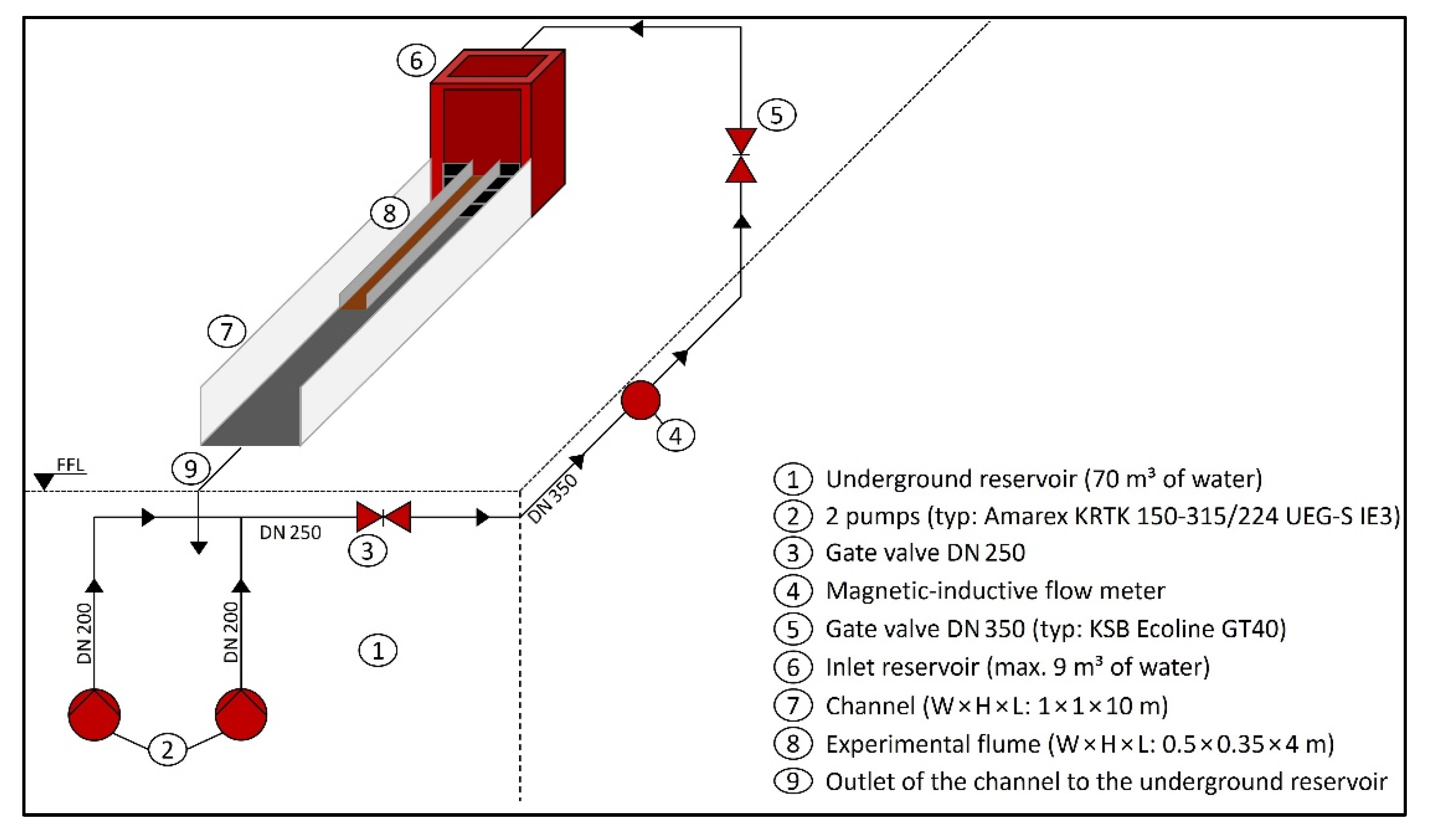
To investigate different degrees of bed roughness depending on the water depth and bottom slope, laboratory experiments were carried out. All experiments were conducted at the laboratory of hydraulic engineering at the University of Applied Sciences in Saarbrücken, Germany. Figure 1 shows a sketch of the closed water circuit that proceeds with the experiments; 70 m³ water is stored in an underground reservoir (Figure 1, no. 1) and is transported by two pumps through a pipe system to an inlet reservoir and the experimental setup. The channel (Figure 1, no. 7) is 10 m long and contains a cross-section of 1 m × 1 m without any slope. At the transition of the inlet reservoir to the channel, a flood protection system is installed to separate both elements. This system is composed of several beams to dam the water in the reservoir to different heights.
For the experiments of this study, a second, smaller channel, the experimental flume (Figure 1, no. 8), was installed. The experimental flume has a length of 4 m and a cross-section of 0.5 m × 0.35 m. Its bottom is a coated plywood plate, and the walls are made of aluminum. For the roughness experiments, the whole bottom was covered with insets. The experimental flume is stabilized at the upstream end of the flume to a handle at the topmost beam of the flood protection system and can therefore align the slope. With the help of a mobile crane at the downstream end of the flume, the slope can be further adjusted. A digital clinometer is supposed to measure the flume’s slope with a precision of 1%. For the entire setup, a range of slopes from 0% to a maximum of 40% (21.8°) is possible (see Figure 2f). The flume is charged by the inlet reservoir, which reduces the turbulence of the flow. A perforated plate evenly conducts the water stream over the whole width of the flume.
In the experimental procedures, the discharge was controlled by gate valves (Figure 1, no. 3 and no. 5) and measured by a magnetic-inductive flow meter (Figure 1, no. 4). The measurements of the water depth were conducted with a point gauge that signals (visually and acoustically) contact with water (Richter Deformationsmesstechnik GmbH, Frauenstein, Germany). A frame with the point gauge was positioned in the middle of the flume to avoid an influence from the inlet and outlet areas. The position was determined by preliminary tests. Water depths were measured in a longitudinal section of the experimental flume, and areas influenced by inlet and outlet were detected. For the final experiments, water depth values are single measurements. When vegetation stalks were higher than the flume walls (Figure 2b), the stalks were slightly bent at the top to fit through openings of the frame. Then, the water depth was measured as in previous experiments using the acoustics of the point gauge when water was touched.
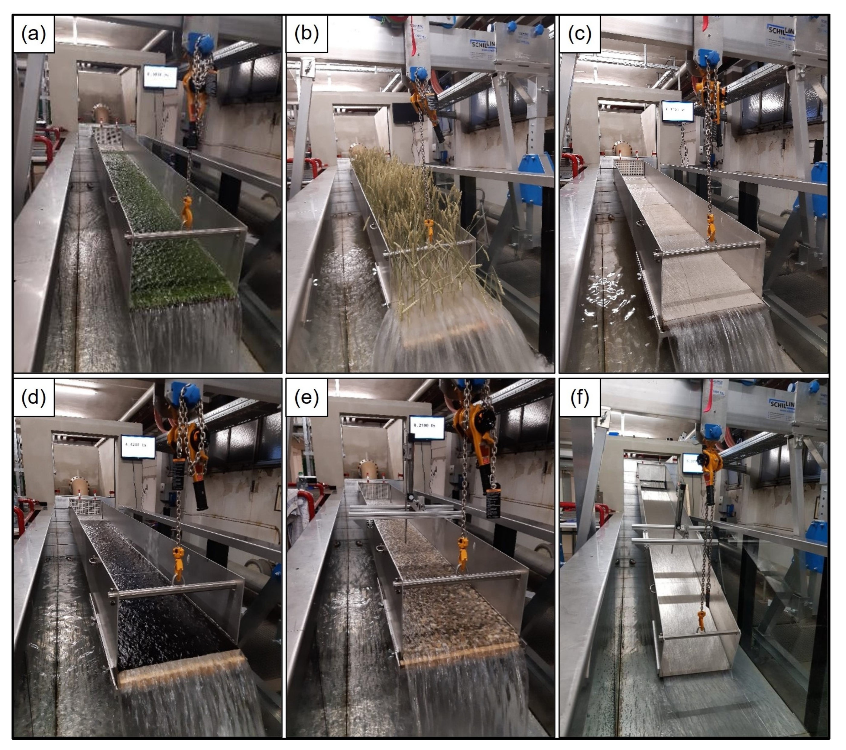
As the objective of this study was to investigate different degrees of bed roughness, the sidewall influence of the flume must be considered. As a preliminary test, aluminum plates were used as insets (Figure 2f). Hence, in addition to the flume walls, the whole experimental flume is covered with aluminum so the material specific roughness can be determined to take the wall roughness for all subsequent experiments into consideration. For the results of bed roughness, wall roughness is considered via the wetted perimeter to use only the specific bottom friction for analyses. All bed roughness and surfaces used in this study are illustrated in Figure 2.
In the present study, flow above solid surfaces as well as flow through and above vegetation is investigated. Artificial grass represents submerged vegetation with a flow above the vegetational layer. For experiments with wheat, the water flows through the wheat stalks, so it is defined as emergent vegetation. Further surfaces are described as “solid”. For each surface, a short description of the configuration details, flow conditions and the range of discharges, water depths and bottom slopes are given in Table 1.

Table 1.
Experimental configurations.
| Reference | Artificial Grass | Wheat | Cement-Based Coating | Asphaltic Emulsion | Exposed Aggregate Concrete | Aluminum | |
|---|---|---|---|---|---|---|---|
| Description | Nubby blade of grass: length: 2.5 cm height: 1.5 cm predominantly rigid | Dried wheat height: 0.5 m 500 pc./m2 fixed in 3 cm Styrodur and on top: 2 cm cement-based coating predominantly rigid (bending was avoided) | Mixture of masonry mortal and tile adhesive (ratio 1:2) | Grain size: 0–8 mm | Texture: gravel; grain size: 5–20 mm | Plates, 2 mm thick | |
| Installation | Sticked and tightened to a coated plywood plate | 4 separate boxes | 4 separate boxes | 4 separate boxes | 4 pieces | 4 pieces sealed with silicone | |
| Flow condition | Submerged vegetation Submergence: 2.1–7.5 | Emergent vegetation | Submerged Solid surface | Submerged Solid surface | Submerged Solid surface | Submerged Solid surface | |
| Total number of experiments | 149 | 77 | 168 | 119 | 119 | 98 | |
| Q [l/s] | 5–70 | 5–35 | 5–70 | 5–70 | 5–70 | 5–70 | |
| h [cm] | 3.1–11.2 | 1.2–14.3 | 1.0–9.5 | 1.1–7.1 | 1.3–7.5 | 0.9–8.0 | |
| Re | 2.48 × 10⁴– 3.31 × 10⁵ | 2.75 × 10⁴– 1.76 × 10⁵ | 2.78 × 10⁴– 3.75 × 10⁵ | 2.65 × 10⁴– 3.64 × 10⁵ | 2.63 × 10⁴– 3.60 × 10⁵ | 2.92 × 10⁴– 3.74 × 10⁵ | |
| S [%] | 1 | X | X | X | X | X | X |
| 2 | X | X | X | ||||
| 3 | X | X | X | ||||
| 4 | X | X | X | ||||
| 5 | X | X | X | X | X | X | |
| 10 | X | X | X | X | X | X | |
| 15 | X | X | X | X | X | X | |
| 20 | X | X | X | X | X | X | |
| 25 | X | X | X | X | X | ||
| 30 | X | X | X | X | X | X | |
| 35 | X | X | X | X | X | ||
| 40 | X | X | X | X | X | ||
4. Results and Discussion
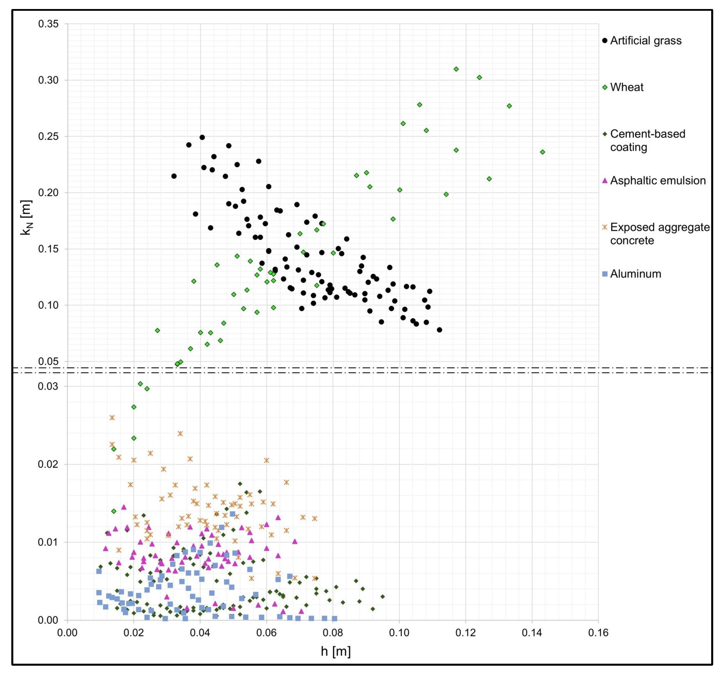
For the analysis of experiments, Darcy–Weisbach’s friction factor f was used because it is the only dimensionless resistance coefficient and valid for all states of flow [17,18]. With the results of the measured discharge, water depth and slope and given boundary conditions of the experimental flume, all parameters are available to calculate f with Equation (1) and kN of each experiment with calculated f and Equation (2). Figure 3 summarizes the data of all types of bed roughness in this study with slopes from 1% to 20%. For this first overview, no distinction is made between solid or vegetation bed roughness, and for every experiment, coefficient kN is considered as bed roughness to show the range of values. For further analyses, the friction factor f or coefficient kN is used, depending on the surface. The plot depicts the dependence of water depth on roughness kN. With a split y-axis, the range of data points for low kN values can be better recognized. For submerged vegetation (artificial grass), roughness decreases with increasing water depth and submergence. In contrast, for emergent vegetation (wheat), roughness increases with increasing water depth. These results of change in roughness depending on submergence are plausible regarding results from the literature for vegetation in the channel [40] and for overland flow [14,17]. Solid surfaces (cement-based coating, asphaltic emulsion, exposed aggregate concrete and aluminum) show a much smoother roughness with a reasonable constant roughness coefficient kN.
By conducting experiments with 1% (independent of bed roughness), discharge losses were noticed at the inlet of the experimental flume. These losses could not be completely avoided, and quantity could only be approximated. Therefore, the measured discharge for all experimental data of slopes = 1% was reduced by 10%.
In addition to the investigation of water depth, the second part of this experimental study was to investigate if and how roughness is influenced by bottom slope. For each bed roughness, a range of different slopes was used as the experimental setup. A list of slope configurations for each experiment is contained in Table 1.
4.1. Consideration of Roughness for Submerged Vegetation
4.1.1. Analyses and Evaluation of Experimental Results
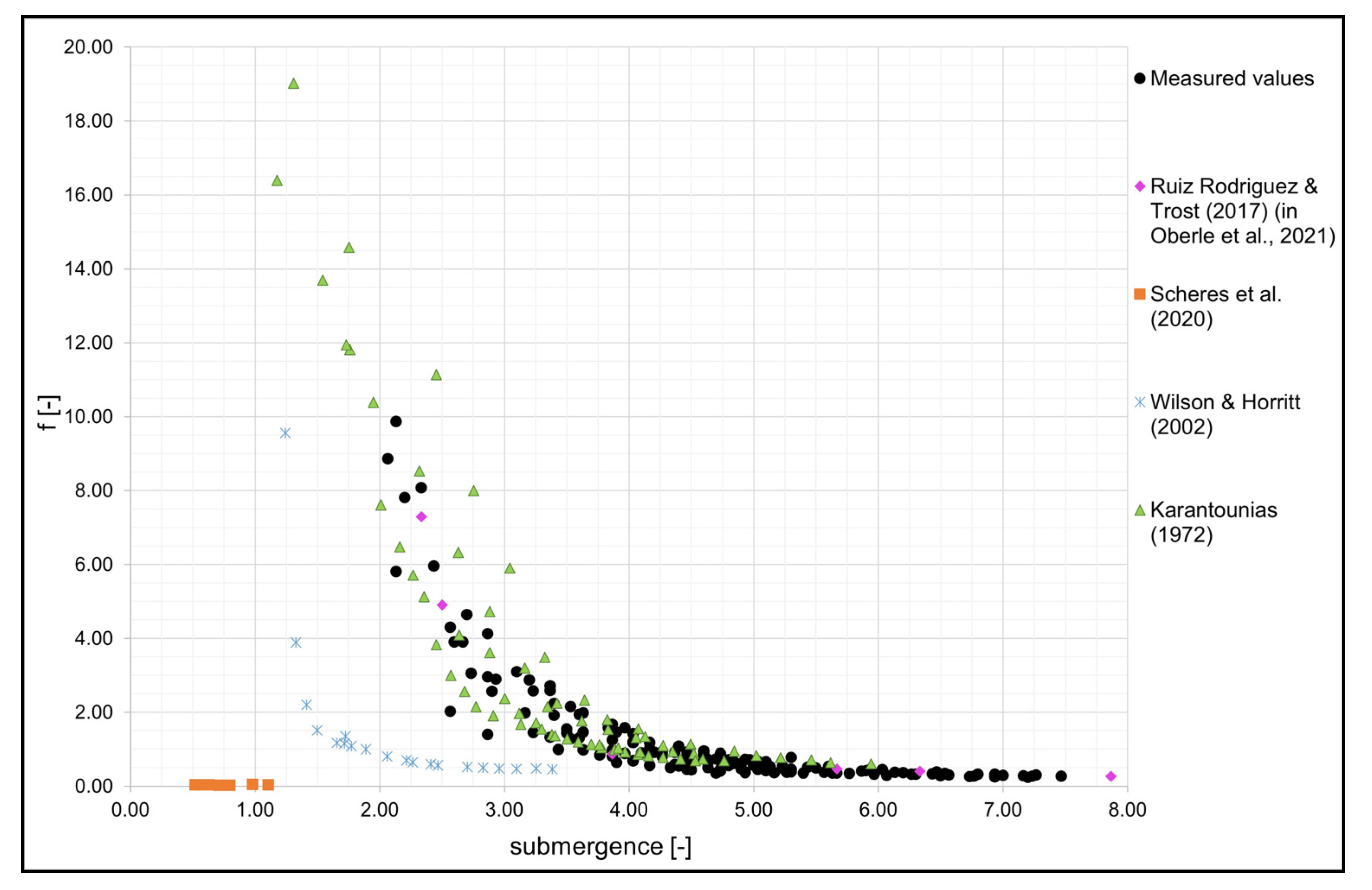
Figure 3 shows that submerged vegetation, in this study artificial grass, leads to a rougher surface with decreasing water depths. Thus, roughness decreases with higher submergence. Previous studies have investigated (artificial) grass with different blade heights and slopes. A comparison of data from this study with data from previous studies is illustrated in Figure 4. All data are shown in terms of relative submergence (h/hveg). The experiments of Ruiz Rodriguez and Trost [58,59] with artificial grass are comparable to the surface used in this study. Accordingly, the data points largely agree with the measurements of this study. Scheres et al. [60] observed a smoother surface for a “species-poor grass-dominated mixture” with a vegetation coverage of 82%. The friction factor for these experiments deviates widely from the results of this study. Here, friction factors are constant for all submergence ratios, and in total, values are lower. Experiments by Wilson and Horritt [61] were carried out in a flume with a bottom slope of 1% and grass blades of 7 cm height. A curve of friction factors for different submergence is given, although data points show lower friction factors for a given submergence than data from the literature. In a study by Karantounias [62], he used a grass mat with blades, which were 8 cm long and bent to the ground. Unfortunately, the height of the vegetation layer was not reported, but one photo was presented. For comparison in Figure 4, a height of 1 cm was assumed to calculate submergence. With this assumption, the results of this study also fit the results of the present study. By increasing the assumed vegetation height, the data points slide to the left. For all data, friction factors are highest for minimum submergence. Reports by Nepf [40] and Abrahams et al. [14,17] and the results of wheat in this study indicate that the curve changes with a submergence of 1 (change from submerged to emergent). Hence, the maximum roughness is reached with submerged vegetation (submergence = 1). With this knowledge, an assumption of a vegetation height of 1 cm for experiments by Karantounias seems plausible because a submergence of 1 is not exceeded.
According to Augustijn et al. [16], Gualtieri et al. [26] and Huthoff et al. [31], roughness approaches a constant value when water depth is much higher than vegetation height. In the mentioned literature, a submergence higher than 5 is stated. The results of the present study indicate constant roughness from a submergence higher than 6 or 7.
Apart from Scheres et al. [60], all experimental data of submerged vegetation from the literature show a similar dependence of submergence on roughness. This result is also mentioned by Scheres et al. [60], who state that, contrary to other data from the literature, the friction factor of their study seems independent of submergence. In the comparison shown in Figure 4, the shape of the functions and submergence deviate because of different vegetation properties (density, shape, …). For a given submergence, data from Wilson and Horritt [61] show lower resistances than the compared data. Against the submergence ratios for constant hydraulic resistance stated by Augustijn et al. [16], Gualtieri et al. [26] and Huthoff et al. [31], data from Wilson and Horritt [61] seem to reach a constant value from a submergence of 3. This phenomenon, which does not fit with other literature data, is also mentioned by Wilson and Horritt themselves. One possible explanation is the flexibility of 7 cm high grass compared to heights of 1 or 2 cm.
Figure 4 shows that the dependence of water depth and roughness for submerged vegetation is known in the literature and thus, these data validate our experiments. In addition to the water depth, the dependence of the bottom slope was investigated. These results are shown and discussed at the end of Section 4.1.3.
To reproduce measured values with a model, different approaches that consider vegetational properties are available.
4.1.2. Existing Models
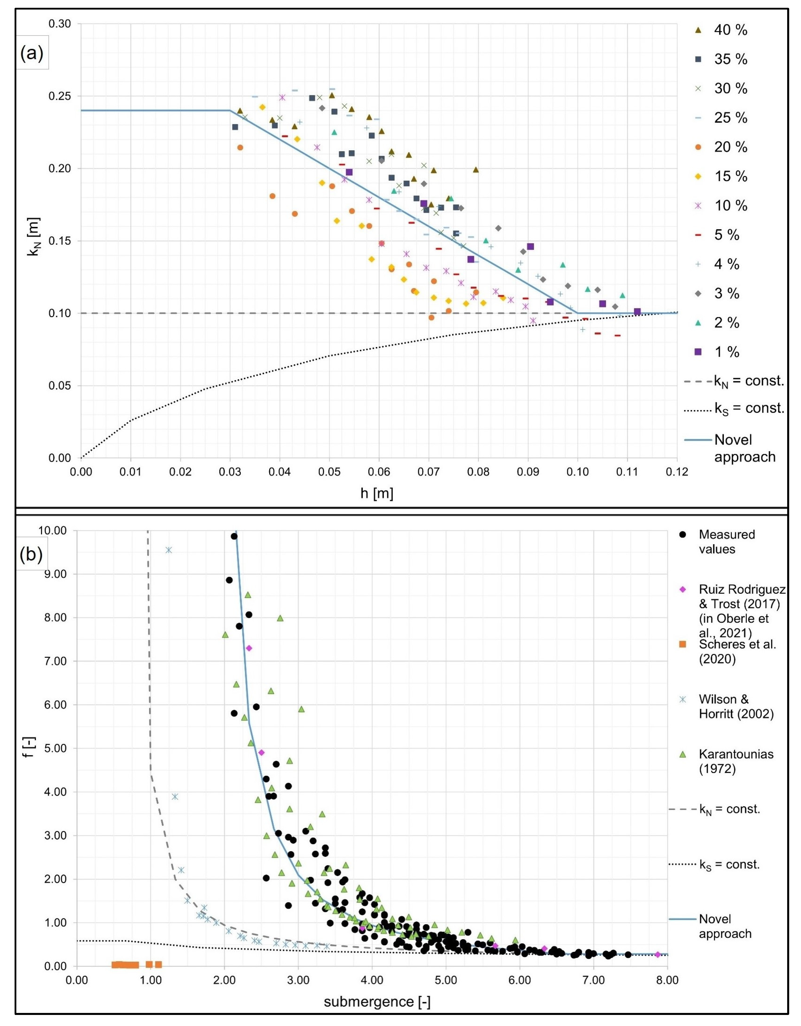
There are several experiments and analyses to consider submerged vegetation, mentioned in the Background section. With vegetation properties of artificial grass used in the present study, approaches lead to the following constant kN values: Gualtieri et al. [26]: 0.205 m; Huthoff [27]: 0.017 m; Schröder [37]: several meters. The kN value from the approach by Schröder [37] strongly deviates from the experimental results of this study, whereas values from the approaches by Gualtieri et al. [26] and Huthoff [27] reproduce the mean values of the experimental data (see Figure 3 and Figure 5a). However, the kN value resulting from the approach by Gualtieri et al. [26] should be valid for submergence ≥5 when hydraulic resistance reaches a constant value. In this study, a constant value of kN = 0.1 m is reached for high submergence (see Figure 5a).
According to the approach by Ferro and Guida [38], by choosing the right calibration parameter (0.21 for artificial grass in this study; selected according to the lowest RMSE), measurements fit quite perfectly with this approach because the “measured” friction factor is calculated with the Darcy-Weisbach equation. However, by using water depth and flow velocity in this equation, an initial value problem appears.
Different approaches, suggested in the literature, and data from the literature were compared to the experimental data from this study. In Figure 5, water depth is plotted against kN (Figure 5a) and submergence against f (Figure 5b) for different approaches in comparison to the experimental data. In Figure 5a, experimental data are shown separately for each slope condition, and in Figure 5b, data from this study are shown as black point clouds for better clarity compared to other data. Both plots show a constant kN, f values obtained with a constant kN (gray, dashed line), as suggested in the literature, and kN/f values obtained with a constant kS (black, dotted line), as it is state of the art in 2D models [63]. All kS values are transformed to f with a combination of the Gauckler–Manning–Strickler equation and Darcy–Weisbach equation (Equation (5) in the following paragraph); conversion of f to kN and backward is carried out with Equation (2). Constant kN and constant kS were chosen as values for high submergence, as these values are listed in the literature for channel flow (see paragraph “Vegetation Resistance”) and therefore fit high water depth. For that, the values of kN = 100 mm and kS = 25 m1/3/s represent these conditions. Mean values for kN and kS could fit the experimental data better as a whole, but over- and underestimate specific ranges of values. The influence of water depth for kS in Figure 5a and for kN in Figure 5b arises from the factor of hydraulic radius RH in both transformation equations. The plot depicts that a constant kN as well as a constant kS merely applies with experiments with high water depths (submergence >6 to 7), although constant kN values can represent the quality of the curve progression in Figure 5b. In Figure 5b, it can be seen that data from Scheres et al. [60] fit with a constant kS and data from Wilson and Horritt [61] fit with a constant kN. Furthermore, Wilson and Horritt conducted experiments with grass blades of 7 cm. If these blades bend, submergence rises, and the curve of data points from Wilson and Horritt approximates the data curve from this study. Properties, especially the density of vegetation, deviate in each experiment, so different values for hydraulic resistance are reasonable.
In the literature, the dependence of vegetation bed roughness and water depth has been reported. However, the friction factor f always depends on the water depth because of the factor RH in Equation (2). Nevertheless, an additional dependence of kN and water depth is shown in Figure 5a. According to these findings, a novel approach for kN depending on water depth is introduced.
4.1.3. Novel Approach
As shown in Figure 5a, roughness coefficient kN is dependent on water depth. This dependence can be described with a linear approach (Figure 5, blue, solid line) in Equation (4).
Equation (4) for kN consists of three parts: (a) a part for submergence ≤1, (b) a part for high submergence and (c) a part for the intermediate area. For submergence ≤1 (h ≤ hveg), the conditions change to emergent, and the hydraulic response is different. To simplify the novel approach, the roughness coefficient kN for h ≤ hveg is assumed to be constant (kN-S1). For water depths with high submergence (h >> hveg or submergence ≥5), a constant value (kN) can be assumed as well [6,16,31]. For the intermediate area, kN will be changed approximately linearly between kN-S1 and kN. This valid range of values is constrained by the minimum kN for high submergence and the maximum kN-S1 for low submergence. The change in roughness for 1 < h/hveg < 5 to 7 depends on the gradient ΔkN/Δ submergence and therefore on the water depth.
The experimental setup of this study was limited to a minimum discharge of 5 L per second, which led to a water depth >3 cm. With a vegetation height of 1.5 cm, a submergence of 1 could not be reached. Due to the lack of knowledge in this range of values, a constant kN for water depths <3 cm was assumed for all the following analyses (as shown in Figure 5a, blue line).
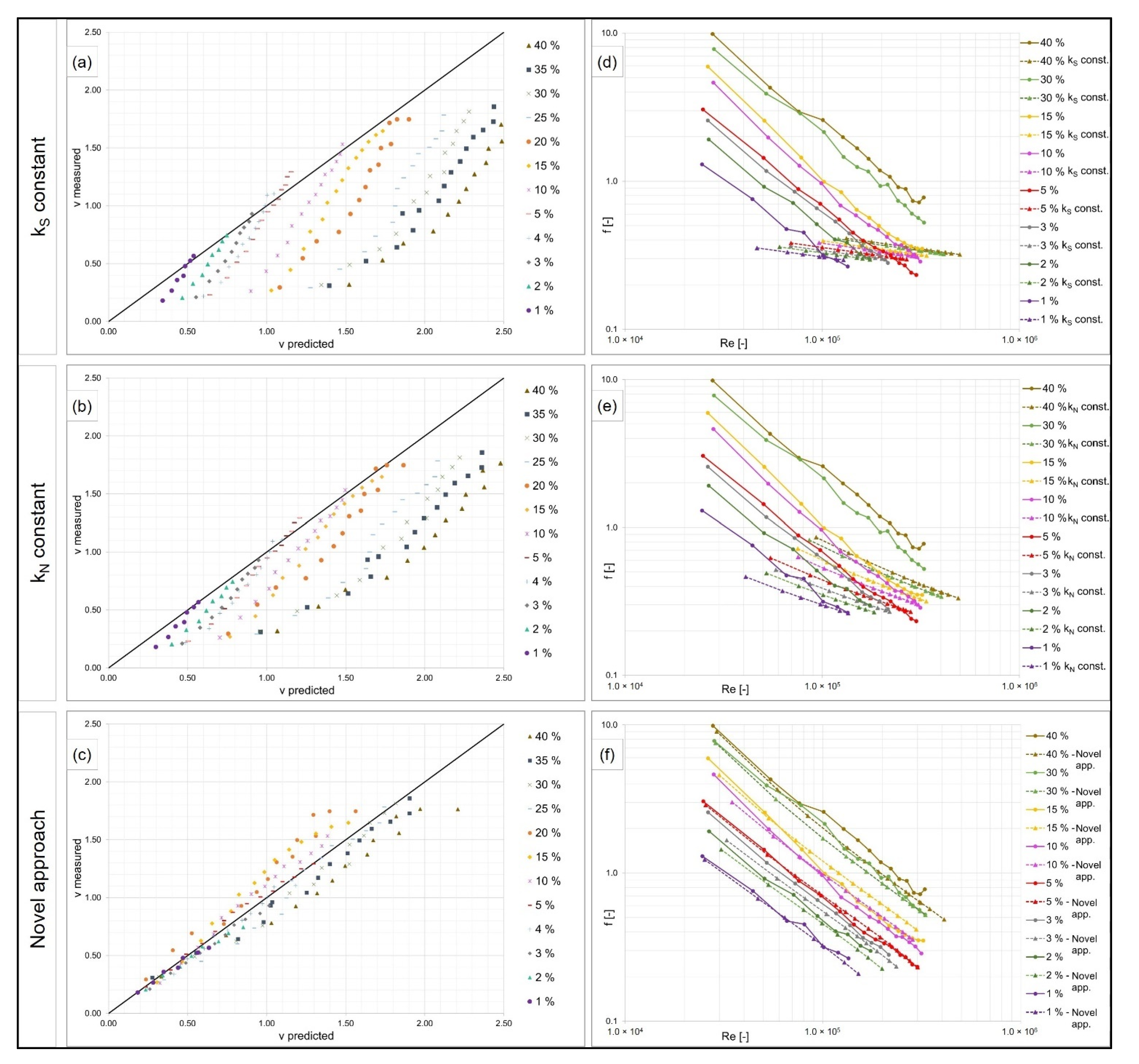
In addition to the evaluation of the appropriate course with water depth vs. kN and submergence vs. f (Figure 5), a comparison of the predicted velocity to the measured velocity (calculated with measured discharge and water depth) for all approaches is shown in Figure 6a–c. For kS = 25 m1/3/s = constant (a) and kN = 0.1 m = constant (b), approaches approximate measured values for high velocities and therefore for high water depths. For data with high bottom slopes, the approaches fit less well. The root mean square error (RMSE) of flow velocity v is 0.463 for kN = constant and 0.604 for kS = constant. Altogether, both approaches lead to velocities that are too high. In the right column of Figure 6d–f, the plot Reynolds number Re against friction factor f indicates the same trend. Accordingly, both approaches cause friction factors that are too small for the predicted scenario (dashed lines). For the novel approach (bottom row), the velocity fits well for small values; for higher velocities, the values scatter (Figure 6c). The RMSE of velocity v is 0.138 for all measurements and 0.094 for v < 1 m/s. The friction factor f can be predicted more precisely than with constant approaches (Figure 6f). Here, an RMSE of 0.57 can be reached for all measurements.
Apart from the influence of water depth on roughness, the bottom slope was investigated. For artificial grass, slopes from 1% to 40% were set. Comparisons of roughness (f/kN) with water depth or submergence do not show clear dependence. From Figure 5a, it can be assumed that roughness increases with decreasing slope for a given water depth. However, some slopes deviate, e.g., 1% and 25% to 40%. The plot of Re vs. f (Figure 6f) shows that the friction factor can be predicted adequately with kN depending on the water depth, and an additional dependence on the bottom slope is not necessary.
As described in the “Modeling Extreme Events” section, considering roughness is an important input and calibration factor for 2D models to calculate water depth and flow velocity and thus to simulate the intensity and temporal course of flood waves at certain points of interest. Therefore, consideration of the correct roughness coefficient is essential. In the following, approaches kS = constant, kN = constant and the novel approach were used in a flash flood simulation to evaluate their effects in a real catchment area.
4.1.4. Implementation in a 2D Model
As one objective of this study is the usage and influence of roughness in simulations, the consideration of roughness in the HydroAS model [64], which is standard software for flood simulation in Germany and neighboring countries, should be introduced.
HydroAS is a two-dimensional hydrodynamic numerical model for simulations of channel flows and flash floods. In contrast to 1D calculations, which include merely the flow velocity and acceleration in the flow direction (x-direction), two-dimensional models calculate the upstream-downstream and transverse direction of the stream (x- and y-direction). The fundamental principle of this model is the utilization of shallow water equations [65].
The simulations of the HydroAS models are influenced by roughness coefficients for every compiled land usage. Modelers can input the value as Strickler roughness kS, either as a constant value or a value depending on the water depth. The programming code of the model converts the Strickler roughness coefficient kS into the friction factor f by merging the Gauckler–Manning–Strickler equation and Darcy–Weisbach equation into the following equation [65]:
In this case, DH represents the hydraulic diameter, with DH = 4 × RH. According to Hydrotec [65], the factor RH can be replaced by water depth for 2D shallow water equations.
To investigate the effect of the approaches proposed in the previous paragraph on the hydrograph in the catchment area, all approaches must be implemented into the model. The sand–grain roughness kN is converted to friction factor f by using Equation (2) and then to Strickler’s roughness coefficient kS with Equation (5). For kN = constant and for the novel approach (Equation (4)), the entered values of kS are a function of water depth. Within the analysis of flash flood simulations, attention is mostly focused on the simulation results of water depth and flow velocity.
By using approaches for submerged vegetation with the Darcy–Weisbach equation, as presented in the previous paragraph (Figure 6), water depth is the only factor used to calculate kN and derive the friction factor f and flow velocity. Thus, appropriate discharge for water depth and velocity is not considered. However, in 2D modeling, discharge or precipitation are initial parameters for simulations. To estimate the influence of this condition, the experimental flume was rebuilt as a 2D model, approaches were applied, and discharge from experiments was used as the initial condition. In Figure 7, measured flow velocities are compared to velocities from manually calculated approaches (a–c) and to velocities from simulations (d–f). Figure 7a–c are extracts from Figure 6a–c. For this comparison, exemplary slopes of 3%, 5%, 15% and 40% were used. This selection represents the total range of values for scattering.
By using a 2D model with roughness approaches and given discharge from measurements, flow velocity is calculated more accurately than manually calculated velocities, and scattering can be reduced. As a result, RMSE improves. For selected data (3, 5, 15 and 40%), RMSE for v predicted (manually) is 0.61 compared to 0.30 for the 2D model with kS = constant; with kN = constant 0.47 against 0.19 and with novel approach, 0.16 against 0.06. Experimental runs with slopes of 40% and low discharge do not bring plausible results with the 2D model and are therefore excluded from Figure 7. Water depth and flow velocity seem unstable. The reason for this is the usage of shallow water equations in 2D simulations. As presented in the introduction of the HydroAS model, only the x- and y-directions are considered for simulation, and the z-direction is not calculated. For very high slopes, such as 40% in experimental runs, conditions of high slopes and low water depth could result in resilient simulation values. However, the analysis of slopes with SRTM1 data (shuttle radar topography mission) shows a share of less than 2% for slopes of 40% and higher for the area of Germany. Consequently, a combination of the mentioned conditions is rare.
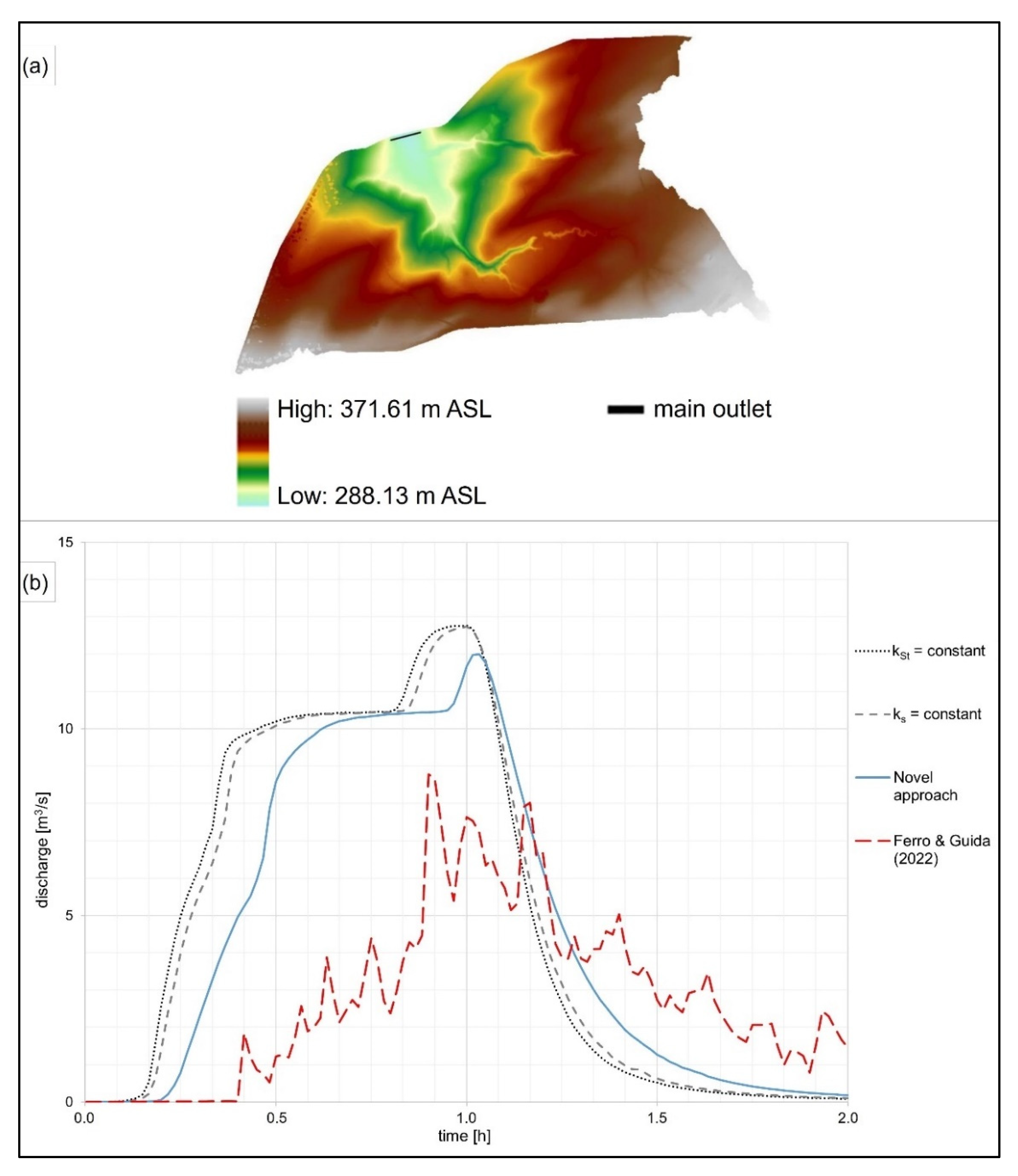
By simulating the experimental flume and comparing the results of the simulated and measured flow velocities, the plausibility check shows improvement compared to the manual calculation. To evaluate the effect of different approaches in a real catchment area, a 2D model was built with a DEM (Figure 8a).
The model used for the following enquiry comprises an area of 1.1 km2, and the elevation varies from 288.13 m to 371.61 m above sea level. In the model, there is no deviation in different land uses, so grassland approaches were applied for the entire model. This method was selected to avoid interactions with different roughness values and other processes. Hence, the discharge curve only results from different grassland approaches to evaluate their effects. Precipitation was considered with an intensity of 60 mm/h for a duration of one hour, and initial losses were taken into account at 2.5 mm. For all scenarios, the total runoff volume is equal.
With the described model, four simulations with different roughness approaches for grassland were carried out:
- The novel approach of this study (Equation (4)) with kN as a function of water depth was applied.
- The approach of Ferro and Guida [38] with friction factor f as a function of slope, Reynolds number and Froude number was applied. Here, the calibration factor was 0.21, which fits best to the measured values of high water depth in this study.
At the main outlet of the model, different discharge curves are reached. Figure 8b illustrates all scenarios mentioned above. Simulation with kS = constant leads to the earliest and highest discharge peak. The approach with kN = constant results in a similar curve but shows translational motion. Due to a higher friction factor for kN = constant, which is presented in Figure 6, overland flow slows down, and a delayed discharge is plausible. By using the novel approach with even higher roughness, translation and retention effects are clearly visible in the discharge curve. For the roughness approach by Ferro and Guida [38], the 2D model has to use water depth and velocity to calculate roughness in every time step. However, these variables should be calculated in the model with existing default roughness. Consequently, the discharge curve shows strong oscillation, and the model seems unstable. Discharge approximates the shown curves and becomes more stable due to the limitation of different equation parameters, such as Re and Fr. Nevertheless, the range of limitations is difficult to define.
A higher friction value for constant kS and kN would lead to an intensified retention and translation of the discharge curve. However, these values over- or underestimate specific areas in the catchment. The accuracy of the hydrograph does not ensure the correct determination of the hydraulics in the entire model [15]. Therefore, the correct approach for friction is essential for obtaining precise results at each point in the model.
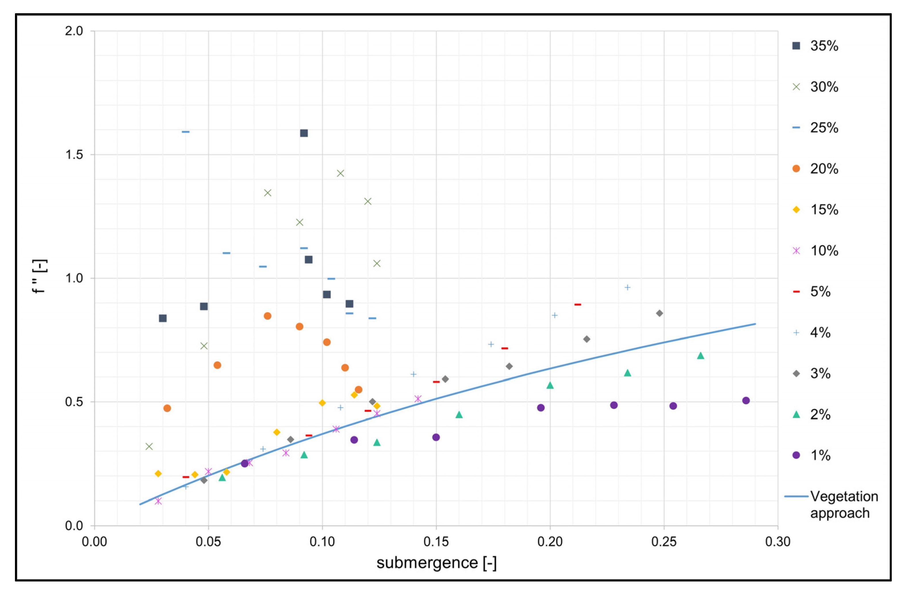
4.2. Consideration of Roughness for Emergent Vegetation
For experiments with emergent vegetation, wheat boxes were constructed. They contain wheat stalks that are 0.5 m high and therefore tower above water depth for each experiment. Each box consists of a bottom layer of Styrodur and a mixture of masonry mortal and tile adhesive to fix wheat stalks. The mortal–adhesive mixture is the same material and therefore has the same surface as the solid surface “cement-based coating” in the “Consideration of Roughness for Solid Surfaces” section.
For the analysis of roughness, total friction must be considered for the bottom layer of the cement-based coating (f′) and further for the vegetation layer of wheat stalks (f″), as described in the “Vegetational Resistance” section. To calculate friction, the results of the experiments with cement-based coating are suitable considering the bottom friction f′. Wheat stalks are considered with a separate vegetation approach for f″ (Equation (3)). The sum of both roughness parts leads to the total resistance f.
The vegetation approach (Equation (3)) considers two parameters that depend on specific vegetational properties. The first is the drag coefficient CD, which is an empirically determined value. In this study, the shape of a cylinder is assumed for wheat stalks, and therefore, a value for CD of 1.2 is selected [21]. The second parameter is the specific frontal area of the vegetation in the x-direction. Due to the experimental setup of this study, a mean diameter of wheat stalks of 3.7 mm and a density of vegetation of 500 pieces/m2 were used for calculation.
To compare the vegetation approach and data from experiments, the experimental results must be adjusted. For each experiment, a total f can be derived from the measured discharge, water depth and slope with the Darcy Weisbach equation (Equation (1)). Part of the bottom resistance f′ was calculated with Equation (2) in combination with a constant kN derived from experiments with a cement-based coating. Here, the approach was simplified by an assumption of kN = 0.006 m as a uniform value for each experiment. Scattering of results from experiments with cement-based coating was not considered. However, the influence of the bottom friction f’ is almost insignificant because the values for kN vary from 2.3 mm to 10.2 mm (see section “Consideration of Roughness for Solid Surfaces”) and therefore f′ varies from 0.05 to 0.1. However, f″ varies from 0.1 to 0.8 (Figure 9). Part of the vegetational resistance f″ was calculated by subtracting f and f′.
Figure 9 shows the share of f″ for the measured data of wheat in comparison to the vegetation approach (Equation (3)) from the literature. For data points with slopes from 1% to 15%, the friction factor f″ increases with increasing submergence. According to Nepf [40] and Abrahams et al. [14,17], this behavior is plausible for emergent vegetation. In contrast, the data points of high bottom slopes (20–35%) vary widely. To reproduce the measured values, a vegetation approach was used. For slopes up to 15%, the curve of this approach lies in the mean range of data scatter. For low submergence with values <0.10, the vegetational approach represents the measured data well. Here, the RMSE of f″ is 0.045. The higher the submergence is, the higher the scattering. For all data of slopes 1–15%, RMSE is 0.112. Data scatters for high velocities and water depth. This is possibly caused by measurement errors due to turbulence. For slopes >15%, the data points do not show an increase in f″ with an increase in submergence. Scattering is strong and results in a total RMSE for f″ of 0.488.
By examining all results regarding slope, no clear dependence can be established. For slopes from 1% to 5%, for a given submergence, the friction factor increases with slope. However, slopes of 10% and 15% do not continue this trend. In total, for experiments of this study with slopes up to 15%, a mean value can be reproduced with a vegetation approach and can be used for the consideration of emergent vegetation in model-based simulations.
4.3. Consideration of Roughness for Solid Surfaces
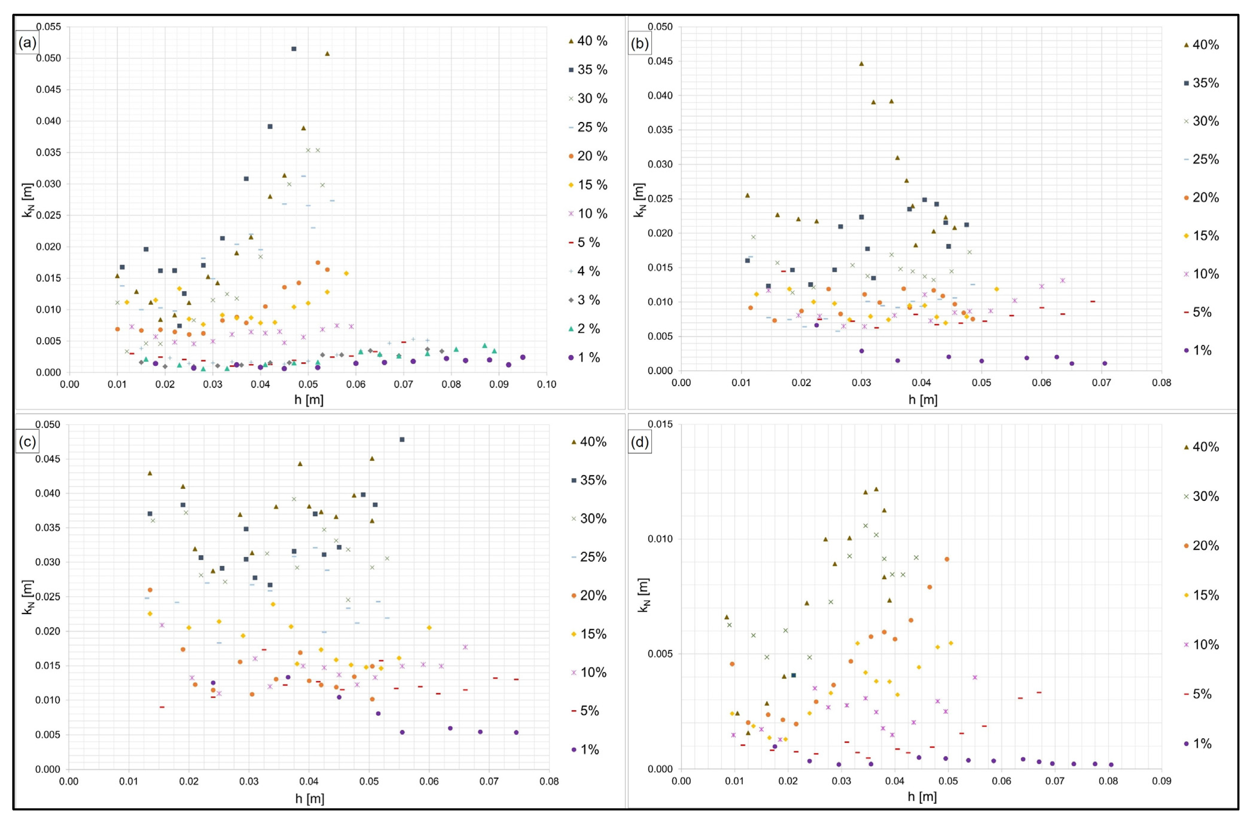
For the category “solid surfaces”, cement-based coating, asphaltic emulsion, exposed aggregate concrete and aluminum were used. Figure 10 shows four plots, one for each material used. Here, water depth is plotted against sand–grain roughness kN to describe bed roughness. In all plots, a similar phenomenon can be perceived. For data of slopes up to 15/20%, the sand-grain roughness kN is an almost constant value for all water depths. This suggests that the roughness coefficient kN does not depend on the water depth. Compared to a condition of constant kN for h >> hveg for submerged vegetation, in this case, water depth is much higher than roughness height kN and therefore, it could be seen as a very high submergence. Against this background, constant kN values seem plausible. For higher slopes, kN scatters or increases with increasing water depth. Similar to the experimental data of the wheat, scattering increases with both bottom slope and water depth. The range of values for the derived kN are listed in Table 2. Here, the mean values for different slope conditions are presented.
The derived kN values of this study are higher than the orders of magnitude listed in the literature. By comparing measured data with data from the literature, it is noticeable that values from the literature often fit within the range of data with slope = 1%. Two explanations are possible: (a) despite the assumption of 90% discharge (see paragraph “Outline”), some data with 1% slope scatter and deviate from the expected curve; perhaps even more discharge was lost, or (b) data from the literature fit with data of 1% slope because literature values are derived from channel conditions with low slopes. Overall, it could be seen that for a given water depth, kN rises with slope. However, this conclusion is weakened by considering scatter due to measurement inaccuracies. By changing the measured water depth by ± 3 mm, kN varies widely by −39 to −60% or rather +53 to +100% (for slopes up to 20%). For comparison of plots shown for submerged vegetation, here, a plot of Re and friction factor (logarithmic display) shows negatively sloping functions with low slopes. This result seems reasonable to what has been reported in the literature [14,17].
5. Conclusions
In this study, laboratory experiments with submerged and emergent vegetation as well as solid surfaces were carried out. As a result of these measurements, different roughness coefficients were derived and analyzed to estimate the influence of water depth and slope on roughness.
For submerged vegetation (artificial grass), the influence of water depth on roughness shows a decrease in roughness with an increase in submergence. The opposite result was observed for emergent vegetation (wheat). Here, a rising submergence leads to a higher roughness. Both results are plausible regarding results from the literature. Due to the submergence of roughness structures, such as vegetation, roughness increases until a submergence of 1, and therefore, its highest roughness is reached. For higher submergence, roughness decreases to a constant value. Analyses of solid surfaces show no dependence of water depth on roughness kN. However, by calculating the friction factor f with the Prandtl–Colebrook equation and a constant kN, the water depth is an influencing factor. Investigations regarding the influence of the bottom slope on roughness show uniform results. In a plot of water depth and roughness kN, the influence of slope could be seen for some data points. Due to scattering, this trend is vague for high slopes and high water depths. However, when considering the friction factor f, the influence disappears or is only slightly visible.
Comparing the results of solid surfaces with results from the literature, constant kN values are reasonable, although the measurements of this study lead, in total, to a slightly higher roughness than presented in the literature. The results of emergent vegetation show that the existing vegetation approach depicts the mean curve for measured values. Scattering rises with increasing water depth and slope. In contrast, the consideration of submerged vegetation is not fully applicable to existing approaches. Consequently, a novel approach appropriate for measured data has been introduced to consider water depth-related roughness. Simulations of an RoG model with different approaches clearly show visible changes in discharge curves. The decision of the roughness approach to correctly calculate water depth and flow velocity has a very high impact on the catchment response. Thus, this response depends on the consideration of the correct roughness value at each point in the entire catchment. To evaluate the quality and decision about the most reasonable approach, real measurements of water level gauges at several points in the catchment area are necessary. For the best model performance, a simple approach is recommended. Calibrated RoG models can be used to simulate specific precipitations and investigate precautions for real flash floods.
The bed roughness investigated in this study was always based on specific surfaces. Other surface structures or vegetational properties lead to different values and approaches. For the vegetation approach of emergent vegetation, properties are considered. For the usage of the proposed, novel approach, the factor ΔkN/Δ submergence should be derived by vegetation properties with data from this study and data from the literature. Thus, further research is needed.
In general, one challenge for modeling flash floods is the knowledge about land use. For given information about, for example, arable land, used roughness is always just a scenario. The surface can be bare soil, or in contrast, fields of wheat, with different stalk heights, depending on the culture and season. Differences in roughness can be immense. At the moment, no increase in roughness with increasing water depth for emergent vegetation is considered in the guidelines [57]. With this approach, wheat fields, as an example of emergent vegetation, could slow overland flow more than currently assumed.
Author Contributions
Conceptualization, A.Y.; methodology, R.H., A.B. and A.Y.; software, R.H. and A.Y.; validation, R.H. and A.Y.; formal analysis, R.H. and A.Y.; investigation, R.H. and A.B.; resources, R.H. and A.B.; data curation, R.H.; writing—original draft preparation, R.H.; writing—review and editing, R.H., A.B. and A.Y.; visualization, R.H.; supervision, A.Y.; project administration, A.Y.; funding acquisition, A.Y. All authors have read and agreed to the published version of the manuscript.
Funding
This research was funded by the University of Applied Sciences, Saarbrücken (BAB_370204513_Sturzflutsimulation) and the state chancellery of the federal state of Saarland (BAB/LFFP 17/13). We acknowledge support by the Deutsche Forschungsgemeinschaft (DFG, German Research Foundation) and Saarland University within the ‘Open Access Publication Funding’ program.
Data Availability Statement
All experimental data of this study are provided at a data repository (doi.org/10.6084/m9.figshare.17142440) [67]. The software HydroAS is commercially available from Hydrotec GmbH, Aachen, Germany (2021b). The simulation model is available as part of a previous project of flash flood simulations in the municipality of Eppelborn [68].
Acknowledgments
The authors thank all students as well as student and scientific assistants, who helped with the construction of the experimental stands and the performance of experiments. Thank you to Eva Loch for her programming expertise in HydroAS.
Conflicts of Interest
The authors declare no conflict of interest. The funders had no role in the design of the study; in the collection, analyses or interpretation of data; in the writing of the manuscript; or in the decision to publish the results.
Limitations
Even though laboratory experiments show, in general, scale invariances to overland flow [34], laboratory experiments offer the possibility of using one bed roughness with different slope settings. In on-site setups, it is nearly impossible to perform experiments with the same bed roughness on different slope sections with slopes ranging from 1% to 40%. During the performance of laboratory experiments, especially for setups with low slopes, some water was leaked after the flow measurement. Although the junction between the reservoir and flume was sealed with foil and duct tape, some loss of flow cannot be ruled out. For slopes = 1%, discharge was adapted to 90% of the measured value.
Notation
| A | Cross-sectional area (m2) |
| CD | Bulk drag coefficient (-) |
| CORR | Corrected |
| DH | Hydraulic diameter (m) |
| dveg | Diameter of the vegetation (m) |
| Dveg | Density of the vegetation (pcs/m2) |
| DEM | Digital elevation model |
| f | Friction factor (Darcy-Weisbach) (-) |
| f′ | Bottom friction factor (-) |
| f″ | Vegetation friction factor (-) |
| Fr | Froude number (-) |
| g | Gravitational acceleration (m/s2) |
| h | Water depth (m) |
| hveg | Vegetation height (m) |
| kN | Equivalent sand-grain roughness (Nikuradse) (m) |
| kS | Strickler roughness coefficient (m1/3/s) |
| pr | Shape coefficient (-) |
| Q | discharge (m³/s) |
| RH | Hydraulic radius (m) |
| Re | Reynolds number (-) |
| RMSE | Root mean square error |
| RoG | Rain-on-Grid |
| S | Channel slope (-) |
| SRTM | Shuttle radar topography mission |
| x | Longitudinal direction along the flume |
| y | Transverse direction of the flume |
| v | Flow velocity (m/s) |
| 2D | Two-dimensional |
References
- IPCC. Summary for Policymakers. In Climate Change 2021: The Physical Science Basis. Contribution of Working Group I to the Sixth Assessment Report of the Intergovernmental Panel on Climate Change; Masson-Delmotte, V., Zhai, P., Pirani, A., Connors, S.L., Péan, C., Berger, S., Caud, N., Chen, Y., Goldfarb, L., Gomis, M.I., et al., Eds.; Cambridge University Press: Cambridge, UK; New York, NY, USA, 2021; pp. 3–32. [Google Scholar] [CrossRef]
- Yörük, A.; Sacher, H. Methoden und Qualität von Modellrechnungen für HW-Gefahrenkarten. In Technische Universität Dresden, Institut für Wasserbau und technische Hydromechanik (Ed.): Simulationsverfahren und Modelle für Wasserbau und Wasserwirtschaft. Dresdner Wasserbauliche Mitt. 2014, 50, 55–64. [Google Scholar]
- Caviedes-Vouillème, D.; García-Navarro, P.; Murillo, J. Influence of mesh structure on 2D full shallow water equations and SCS Curve Number simulation of rainfall/runoff events. J. Hydrol. 2012, 448–449, 39–59. [Google Scholar] [CrossRef]
- Bellos, V.; Papageorgaki, I.; Kourtis, I.; Vangelis, H.; Kalogiros, I.; Tsakiris, G. Reconstruction of a flash flood event using a 2D hydrodynamic model under spatial and temporal variability of storm. Nat. Hazards 2020, 101, 711–726. [Google Scholar] [CrossRef]
- Gibson, M.J.; Savic, D.A.; Djordjevic, S.; Chen, A.S.; Fraser, S.; Watson, T. Accuracy and computational efficiency of 2D urban surface flood modelling based on cellular automata. Procedia Eng. 2016, 154, 801–810. [Google Scholar] [CrossRef] [Green Version]
- Barbero, G.; Costabile, P.; Costanzo, C.; Ferraro, D.; Petaccia, G. 2D hydrodynamic approach supporting evaluations of hydrological response in small watersheds: Implications for lag time estimation. J. Hydrol. 2022, 610, 127870. [Google Scholar] [CrossRef]
- Taccone, F.; Antoine, G.; Delestre, O.; Goutal, N. A new criterion for the evaluation of the velocity field for rainfall-runoff modelling using a shallow-water model. Adv. Water Resour. 2020, 140, 103581. [Google Scholar] [CrossRef]
- Abderrezzak, K.E.K.; Paquier, A.; Mignot, E. Modelling flash flood propagation in urban areas using a two-dimensional numerical model. Nat. Hazards 2009, 50, 433–460. [Google Scholar] [CrossRef]
- Huang, W.; Cao, Z.-x.; Qi, W.-j.; Pender, G.; Zhao, K. Full 2D Hydrodynamic Modelling of Rainfall-induced Flash Floods. J. Mt. Sci. 2015, 12, 1203–1218. [Google Scholar] [CrossRef]
- Costabile, P.; Costanzo, C.; Ferraro, D.; Barco, P. Is HEC-RAS 2D accurate enough for storm-event hazard assessment? Lessons learnt from a benchmarking study based on rain-on-grid modelling. J. Hydrol. 2021, 603, 126962. [Google Scholar] [CrossRef]
- Zeiger, S.J.; Hubbart, J.A. Measuring and modeling event-based environmental flows: An assessment of HEC-RAS 2D rain-on-grid simulations. J. Environ. Manag. 2021, 285, 112125. [Google Scholar] [CrossRef]
- García-Pintado, J.; Barberá, G.G.; Erena, M.; Castillo, V.M. Calibration of structure in a distributed forecasting model for a semiarid flash flood: Dynamic surface storage and channel roughness. J. Hydrol. 2009, 377, 165–184. [Google Scholar] [CrossRef]
- David, A.; Schmalz, B. Flood hazard analysis in small catchments: Comparison of hydrological and hydrodynamic approaches by the use of direct rainfall. J. Flood Risk Manag. 2020, 13, e12639. [Google Scholar] [CrossRef]
- Abrahams, A.D.; Parsons, A.J.; Luk, S.-H. Field experiments on the resistance to overland flow on desert hillslopes. In Erosion, Transport and Deposition Processes, Proceedings of the Jerusalem Workshop, Jerusalem, Israel, March–April 1987; IAHS Publications: Wallingford, UK, 1990. [Google Scholar]
- Cea, L.; Legout, C.; Darboux, F.; Esteves, M.; Nord, G. Experimental validation of a 2D overland flow model using high resolution water depth and velocity data. J. Hydrol. 2014, 513, 142–153. [Google Scholar] [CrossRef]
- Augustijn, D.C.M.; Huthoff, F.; van Velzen, E.H. Comparison of vegetation roughness description. In Proceedings of the International Conferences on Fluvial Hydraulics (River Flow), Izmir, Turkey, 3–5 September 2008; pp. 343–350. [Google Scholar]
- Abrahams, A.D.; Parsons, A.J.; Wainwright, J. Resistance to overland flow on semiarid grassland and shrubland hillslopes, Walnut Gulch, southern Ariona. J. Hydrol. 1994, 156, 431–446. [Google Scholar] [CrossRef]
- Huthoff, F.; Augistijn, D.C.M. Hydraulic Resistance of Vegetation: Predictions of Average Flow Velocities Based on a Rigid-Cylinders Analogy; Final Project Report; Planungsmanagement für Auen, University of Twente: Enschede, The Netherlands, 2006. [Google Scholar]
- Prandtl, L., II. Theoretischer Teil. Zur turbulenten Strömung in Rohren und längs Platten. In Ergebnisse der Aerodynamischen Versuchsanstalt zu Göttingen. IV. Lieferung; Dillmann, A., Ed.; Göttinger Klassiker der Strömungsmechanik: Göttingen, Germany, 2009. [Google Scholar] [CrossRef] [Green Version]
- Nikuradse, J. Strömungsgesetze in Rauhen Rohren; VDI: Berlin, Germany, 1933. [Google Scholar]
- Aigner, D.; Bollrich, G. Handbuch der Hydraulik für Wasserbau und Wasserwirtschaft, 1st ed.; Beuth Verlag GmbH: Berlin, Germany, 2015; ISBN 978-3-410-21341-3. [Google Scholar]
- Chow, V.T. Open-Channel Hydraulics; McGraw-Hill Book Company: New York, NY, USA, 1959. [Google Scholar]
- Zanke, U. Hydraulik für Wasserbau, 3rd ed.; Springer: Berlin/Heidelberg, Germany, 2013. [Google Scholar] [CrossRef]
- Abood, M.M.; Yusuf, B.; Mohammed, T.A.; Ghazali, A.H. Manning Roughness Coefficient for Grass-Lined Channel. Suranaree J. Sci. Technol. 2006, 13, 317–330. [Google Scholar]
- Ferro, V. Assessing flow resistance law in vegetated channels by dimensional analysis and self-similarity. Flow Meas. Instrum. 2019, 69, 101610. [Google Scholar] [CrossRef]
- Gualtieri, P.; De Felice, S.; Pasquino, V.; Doria, G.P. Use of conventional flow resistance equations and a model for the Nikuradse roughness in vegetated flows at high submergence. J. Hydrol. Hydromech. 2018, 66, 107–120. [Google Scholar] [CrossRef] [Green Version]
- Huthoff, F. Theory for flow resistance caused by submerged roughness elements. J. Hydraul. Res. 2012, 50, 10–17. [Google Scholar] [CrossRef]
- Nepf, H.M.; Vivoni, E.R. Flow structure in depth-limited, vegetated flow. J. Geophys. Res. 2000, 105, 28547–28557. [Google Scholar] [CrossRef]
- Tang, X.; Wu, S.; Rahimi, H.; Xue, W.; Lei, Y. Experimental Study of Open Channel Flows with Two Layers Vegetation. In Proceedings of the 2nd International Symposium on Hydraulic Modelling and Measuring Technology Congress, Nanjing, China, 30 May–1 June 2018. [Google Scholar]
- Wang, W.-J.; Peng, W.-Q.; Huai, W.-X.; Katul, G.G.; Liu, X.-B.; Qu, X.-D.; Dong, F. Friction factor for turbulent open channel flow covered by vegetation. Sci. Rep. 2019, 9, 5178. [Google Scholar] [CrossRef] [Green Version]
- Huthoff, F.; Augistijn, D.C.M.; Hulscher, S.J.M.H. Analytical solution of the depth-averaged flow velocity in case of submerged rigid cylindrical vegetation. Water Resour. Res. 2007, 43, W06413. [Google Scholar] [CrossRef] [Green Version]
- Järvelä, J. Determination of flow resistance cause by non-submerged woody vegetation. Int. J. River Basin Manag. 2004, 2, 61–70. [Google Scholar] [CrossRef]
- Vargas-Luna, A.; Crosato, A.; Uijttewaal, W.S.J. Effects of vegetation on flow and sediment transport: Comparative analyses and validation of predicting models. Earth Surf. Process. Landf. 2015, 40, 157–176. [Google Scholar] [CrossRef]
- Ferguson, R. Limits to scale invariance in alluvial rivers. Earth Surf. Process. Landf. 2021, 46, 173–187. [Google Scholar] [CrossRef]
- Baptist, M.J.; Babovic, V.; Rodríguez Uthurburu, J.; Keijzer, M.; Uittenbogaard, R.E.; Mynett, A.; Verwey, A. On inducing equations for vegetation resistance. J. Hydraul. Res. 2007, 45, 435–450. [Google Scholar] [CrossRef]
- Van Velzen, E.H.; Jesse, P.; Cornelissen, P.; Coops, H. Stromingsweerstand Vegetatie in Uiterwaarden; Handboek. Part 1 and 2. RIZA Reports, 2003.028 and 2003.029; Directoraat-Generaal Rijkswaterstaat, RIZA: Arnhem, The Netherlands, 2003. [Google Scholar]
- Schröder, R. Hydraulische Methoden zur Erfassung von Rauheiten; Schriftenreihe des DVWK: Parey, Germany, 1990; Volume 92, ISBN 978-3-490-09297-7. [Google Scholar]
- Ferro, V.; Guida, G. A theoretically-based overland flow resistance law for upland grassland habitats. Catena 2022, 210, 105863. [Google Scholar] [CrossRef]
- Bond, S.; Kirkby, M.J.; Johnston, J.; Crowle, A.; Holden, J. Seasonal vegetation and management influence overland flow velocity and roughness in upland grassland. Hydrol. Process. 2020, 34, 3777–3791. [Google Scholar] [CrossRef]
- Nepf, H.M. Hydrodynamics of vegetated channels. J. Hydraul. Res. 2012, 50, 262–279. [Google Scholar] [CrossRef] [Green Version]
- Polyakov, V.; Stone, J.; Holifield Collins, C.; Nearing, M.A.; Paige, G.; Buono, J.; Gomez-Pond, R.-L. Rainfall simulation experiments in the southwestern USA using the Walnut Gulch Rainfall Simulator. Earth Syst. Sci. Data 2018, 10, 19–26. [Google Scholar] [CrossRef]
- Ferro, V. New Flow-Resistance Law for Steep Mountain Streams Based on Velocity Profile. J. Irrig. Drain. Eng. 2017, 143, 1208. [Google Scholar] [CrossRef]
- Nicosia, A.; Di Stefano, C.; Palmeri, V.; Pampalone, V.; Ferro, V. Flow resistance of overland flow on a smooth bed under simulated rainfall. Catena 2020, 187, 104351. [Google Scholar] [CrossRef]
- Palmeri, V.; Pampalone, V.; Di Stefano, C.; Nicosia, A.; Ferro, V. Experiments for testing soil texture effects on flow resistance in mobile bed rills. Catena 2018, 171, 176–184. [Google Scholar] [CrossRef]
- Carollo, F.G.; Di Stefano, C.; Nicosia, A.; Palmeri, V.; Pampalone, V.; Ferro, V. Flow resistance in mobile bed rills shaped in soils with different texture. Eur. J. Soil Sci. 2021, 72, 2062–2075. [Google Scholar] [CrossRef]
- Di Stefano, C.; Nicosia, A.; Pampalone, V.; Palmeri, V.; Ferro, V. Rill flow resistance law under equilibrium bed-load transport conditions. Hydrol. Process. 2019, 33, 1317–1323. [Google Scholar] [CrossRef]
- Di Stefano, C.; Nicosia, A.; Palmeri, V.; Pampalone, V.; Ferro, V. Comparing flow resistance law for fixed and mobile bed rills. Hydrol. Process. 2019, 33, 3330–3348. [Google Scholar] [CrossRef]
- Di Stefano, C.; Nicosia, A.; Palmeri, V.; Pampalone, V.; Ferro, V. Estimating flow resistance in steep slope rills. Hydrol. Process. 2021, 35, e14296. [Google Scholar] [CrossRef]
- Nicosia, A.; Di Stefano, C.; Pampalone, V.; Palmeri, V.; Ferro, V.; Nearing, M.A. Testing a new rill flow resistance approach using the Water Erosion Prediction Project experimental database. Hydrol. Process. 2019, 33, 616–626. [Google Scholar] [CrossRef]
- Nicosia, A.; Bischetti, G.B.; Chiaradia, E.; Gandolfi, C.; Ferro, V. A full-scale study of Darcy-Weisbach friction factor for channels vegetated by riparian species. Hydrol. Process. 2021, 35, e14009. [Google Scholar] [CrossRef]
- Cheng, N.-S. Representative roughness height of submerged vegetation. Water Resour. Res. 2011, 47, W08517. [Google Scholar] [CrossRef]
- Dunn, C.; López, F.; García, M. Mean Flow and Turbulence in a Laboratory Channel with Simulated Vegetation; Civil Engineering Studies, Hydraulic Engineering Series; University of Illinois: Champaign, IL, USA, 1996. [Google Scholar]
- Murphy, E.; Ghisalberti, M.; Nepf, H. Model and laboratory study of dispersion in flows with submerged vegetation. Water Resour. Res. 2007, 43, W05438. [Google Scholar] [CrossRef]
- Comiti, F.; Mao, L.; Wilcox, A.; Wohl, E.E.; Lenzi, M.A. Field-derived relationships for flow velocity and resistance in high-gradient streams. J. Hydrol. 2007, 340, 48–62. [Google Scholar] [CrossRef]
- Schubert, J.E.; Sanders, B.F.; Smith, M.J.; Wright, N.G. Unstructured mesh generation and landcover-based resistance for hydrodynamic modeling of urban flooding. Adv. Water Resour. 2008, 31, 1603–1621. [Google Scholar] [CrossRef]
- Tyrna, B.; Assmann, A.; Fritsch, K.; Johann, G. Large-scale high-resolution pluvial flood hazard mapping using the raster-based hydrodynamic two-dimensional model FloodAreaHPC. J. Flood Risk Manag. 2018, 11, 1024–1037. [Google Scholar] [CrossRef] [Green Version]
- LUBW Landesanstalt für Umwelt, Messungen und Naturschutz Baden-Württemberg, Publ. Anhänge 1 a, b, c zum Leitfaden Kommunales Starkregenrisikomanagement in Baden-Württemberg. 2020. Available online: https://pudi.lubw.de/detailseite/-/publication/47871 (accessed on 4 December 2022).
- Ruiz Rodriguez, E.; Trost, L. Umgang mit Starkniederschlägen in Hessen. Auszug aus dem 3. Zwischenbericht. KLIMPRAX Starkregen Arbeitspaket 2; Hochschule RheinMain: Wiesbaden, Germany, 2017. [Google Scholar]
- Oberle, P.; Kron, A.; Kerlin, T.; Ruiz Rodriguez, E.; Nestmann, F. Diskussionsbeitrag zur Fließwiderstandsparametrisierung zur Simulation der Oberflächenabflüsse bei Starkregen. WasserWirtschaft 2021, 4, 12–21. [Google Scholar] [CrossRef]
- Scheres, B.; Schüttrumpf, H.; Felder, S. Flow Resistance and Energy Dissipation in Supercritical Air-Water Flows Down Vegetated Chutes. Water Resour. Res. 2020, 56, e2019WR026686. [Google Scholar] [CrossRef] [Green Version]
- Wilson, C.A.M.E.; Horritt, M.S. Measuring the flow resistance of submerged grass. Hydrol. Process. 2002, 16, 2589–2598. [Google Scholar] [CrossRef]
- Karantounias, G. Dünnschichtabfluss auf Stark Geneigter Ebene. Ph.D. Thesis, University Karlsruhe (TH), Karlsruhe, Germany, 1972. [Google Scholar]
- LfU Bayerisches Landesamt für Umwelt, Publ. Handbuch Hydraulische Modellierung. Vorgehensweisen und Standards für die 2-D-hydraulische Modellierung von Fließgewässern in Bayern. 2018. Available online: https://www.bestellen.bayern.de/application/applstarter?APPL=eshop&DIR=eshop&ACTIONxSETVAL(artdtl.htm,APGxNODENR:3779,AARTxNR:lfu_was_00134,AARTxNODENR:351717,USERxBODYURL:artdtl.htm,KATALOG:StMUG,AKATxNAME:StMUG,ALLE:x)=X (accessed on 4 December 2022).
- Software HYDRO_AS-2D, version 5.3.4.; Hydrotec Ingenieurgesellschaft für Wasser und Umwelt mbH: Aachen, Germany, 2022.
- Reference Manual, HYDRO_AS-2D, 2D-Flow Model for Water Management Applications, Version 5.2.5; Hydrotec Ingenieurgesellschaft für Wasser und Umwelt mbH: Aachen, Germany, 2021.
- Albert, A. Schneider–Bautabellen für Ingenieure mit Berechnungshinweisen und Beispielen, 24th ed.; Reguvis: Köln, Germany, 2020; ISBN 978-3-8462-1140-3. [Google Scholar]
- Hinsberger, R.; Biehler, A.; Yörük, A. Influence of Water Depth and Slope on Roughness—Experiments and Roughness Approach for Rain-on-Grid Modeling. Data Repos. 2021. [Google Scholar] [CrossRef]
- Fitt gGmbH, FG Wasser der Htw Saar. Untersuchung der Auswirkungen von Überflutungen Infolge Starkregens für die Gemeinde Eppelborn, Saarbrücken; 2020. Available online: https://www.eppelborn.de/starkregenstudie/ (accessed on 1 December 2022).
Figure 1.
Sketch of the experimental setup.

Figure 2.
Photos of the experimental flume with different surfaces: (a) artificial grass, (b) wheat, (c) cement-based coating, (d) asphaltic emulsion, (e) exposed aggregate concrete, and (f) aluminum.
Figure 2.
Photos of the experimental flume with different surfaces: (a) artificial grass, (b) wheat, (c) cement-based coating, (d) asphaltic emulsion, (e) exposed aggregate concrete, and (f) aluminum.

Figure 3.
Relationship between water depth h and equivalent sand–grain roughness kN for different bed roughnesses. Ordinate was split to better show data points with low kN.
Figure 3.
Relationship between water depth h and equivalent sand–grain roughness kN for different bed roughnesses. Ordinate was split to better show data points with low kN.

Figure 4.
Relationship between relative submergence (h/hveg) and friction factor f. Measured values of this study (black dots) are compared to data from the literature [59,60,61,62].

Figure 5.
Relationship between water depth or submergence and roughness parameters: (a) water depth h against equivalent sand–grain roughness kN with courses of the novel approach (Equation (4)), a constant kN and a constant kS in comparison to measured values of this study (dots, separately for each slope condition) and (b) submergence against friction factor f with courses of the novel approach (Equation (4)), a constant kN and a constant kS in comparison to measured values of this study (black dots) and data from the literature [58,59,60,61,62].

Figure 6.
Comparison of approaches kS = constant, kN = constant and novel approach for quality assurance. (a–c): Comparison of predicted velocity and measured velocity. (d–f): Comparison of Reynolds number Re and friction factor f (logarithmic) for measurements (continuous lines) and predictions (dashed lines).

Figure 7.
Comparison of approaches kS = constant, kN = constant and novel approach, manually calculated and implemented in 2D model. (a–c): Comparison of predicted velocity and measured velocity for 3%, 5%, 15% and 40%. (d–f): Comparison of velocity from the 2D model and measured velocity for 3%, 5%, 15% and 40%.

Figure 8.
Model area and 2D results: (a) DEM of the model and location of the main outlet, (b) hydrograph for different scenarios at the main outlet [38].
Figure 8.
Model area and 2D results: (a) DEM of the model and location of the main outlet, (b) hydrograph for different scenarios at the main outlet [38].

Figure 9.
Relationship between submergence (h/hveg) and friction factor f″ for measured values of experiments with wheat (dots) in comparison to the vegetation approach (blue, solid line, Equation (3)).
Figure 9.
Relationship between submergence (h/hveg) and friction factor f″ for measured values of experiments with wheat (dots) in comparison to the vegetation approach (blue, solid line, Equation (3)).

Figure 10.
Relationship between water depth h and equivalent sand–grain roughness kN for measured values of (a) cement-based coating, (b) asphalt emulsion, (c) exposed aggregate concrete, and (d) aluminum.
Figure 10.
Relationship between water depth h and equivalent sand–grain roughness kN for measured values of (a) cement-based coating, (b) asphalt emulsion, (c) exposed aggregate concrete, and (d) aluminum.

Table 2.
Derived, mean kN values from experiments of this study and literature references.
| Surface | Range of Mean kN Values (For S = 2%–S = 20%) | Literature [66] |
|---|---|---|
| Cement-based coating (Figure 10a) | 2.3–10.3 mm (for slope = 1%: kN = 1.4 mm) | Concrete, smooth: kN = 1–6 mm |
| Asphaltic emulsion (Figure 10b) | 8.3–9.7 mm (for slope = 1%: kN = 2.3 mm) | Asphaltic concrete or mastic asphalt: kN = 1.5–2.2 mm |
| Exposed aggregate concrete (Figure 10c) | 12.4–18.4 mm (for slope = 1%: kN = 8.3 mm) | Concrete smooth—rough: kN = 1–20 mm |
| Aluminum (Figure 10d) | 1.3–4.6 mm (for slope = 1%: kN = 0.4 mm) | Steel: kN = 0.04–0.1 mm |
Publisher’s Note: MDPI stays neutral with regard to jurisdictional claims in published maps and institutional affiliations. |
© 2022 by the authors. Licensee MDPI, Basel, Switzerland. This article is an open access article distributed under the terms and conditions of the Creative Commons Attribution (CC BY) license (https://creativecommons.org/licenses/by/4.0/).
Share and Cite
MDPI and ACS Style
Hinsberger, R.; Biehler, A.; Yörük, A. Influence of Water Depth and Slope on Roughness—Experiments and Roughness Approach for Rain-on-Grid Modeling. Water 2022, 14, 4017. https://doi.org/10.3390/w14244017
AMA Style
Hinsberger R, Biehler A, Yörük A. Influence of Water Depth and Slope on Roughness—Experiments and Roughness Approach for Rain-on-Grid Modeling. Water. 2022; 14(24):4017. https://doi.org/10.3390/w14244017
Chicago/Turabian StyleHinsberger, Rebecca, Andreas Biehler, and Alpaslan Yörük. 2022. "Influence of Water Depth and Slope on Roughness—Experiments and Roughness Approach for Rain-on-Grid Modeling" Water 14, no. 24: 4017. https://doi.org/10.3390/w14244017
Note that from the first issue of 2016, this journal uses article numbers instead of page numbers. See further details here.