
Numerical Investigation of Hydrodynamics in a U-Shaped Open Channel Confluence Flow with Partially Emergent Rigid Vegetation
School of Civil and Hydraulic Engineering, Dalian University of Technology, 2 Ling Gong Road, Dalian 116024, China
*
Author to whom correspondence should be addressed.
Water 2022, 14(24), 4027; https://doi.org/10.3390/w14244027
Submission received: 11 November 2022
/
Revised: 4 December 2022
/
Accepted: 6 December 2022
/
Published: 9 December 2022
(This article belongs to the Special Issue Fluvial Hydraulics in the Presence of Vegetation in Channels)
Abstract
:The effects of partially emergent rigid vegetation on the hydrodynamics of a curved open-channel confluence flow were simulated using OpenFOAM. The numerical model using the Volume of Fluid method and the RNG k-ε turbulence model in the Reynolds-averaged Navier–Stokes equations was first validated by existing experimental data with good agreement. Then the characteristics of hydrodynamics were analyzed in aspects of separation zone, water level, streamwise velocities, secondary flows, bed shear stress and flow resistance. Some main conclusions can be drawn from the results. Compared to the non-vegetated cases, the separation zones in vegetated cases are smaller in both length and width. With higher vegetation Solid Volume Fraction (SVF), the separation zone is divided into two parts, a smaller one right after the confluence point and a larger one on the second half of the curved reach after the confluence. The main circulation cell shrinks and the circulation near the concave bank moves towards the channel midline. The differences in velocities and bed shear stress between the convex and concave banks become larger with a higher SVF. Under the same SVF, a larger vegetation density has more disturbance on the tributary than a larger stem diameter.
1. Introduction
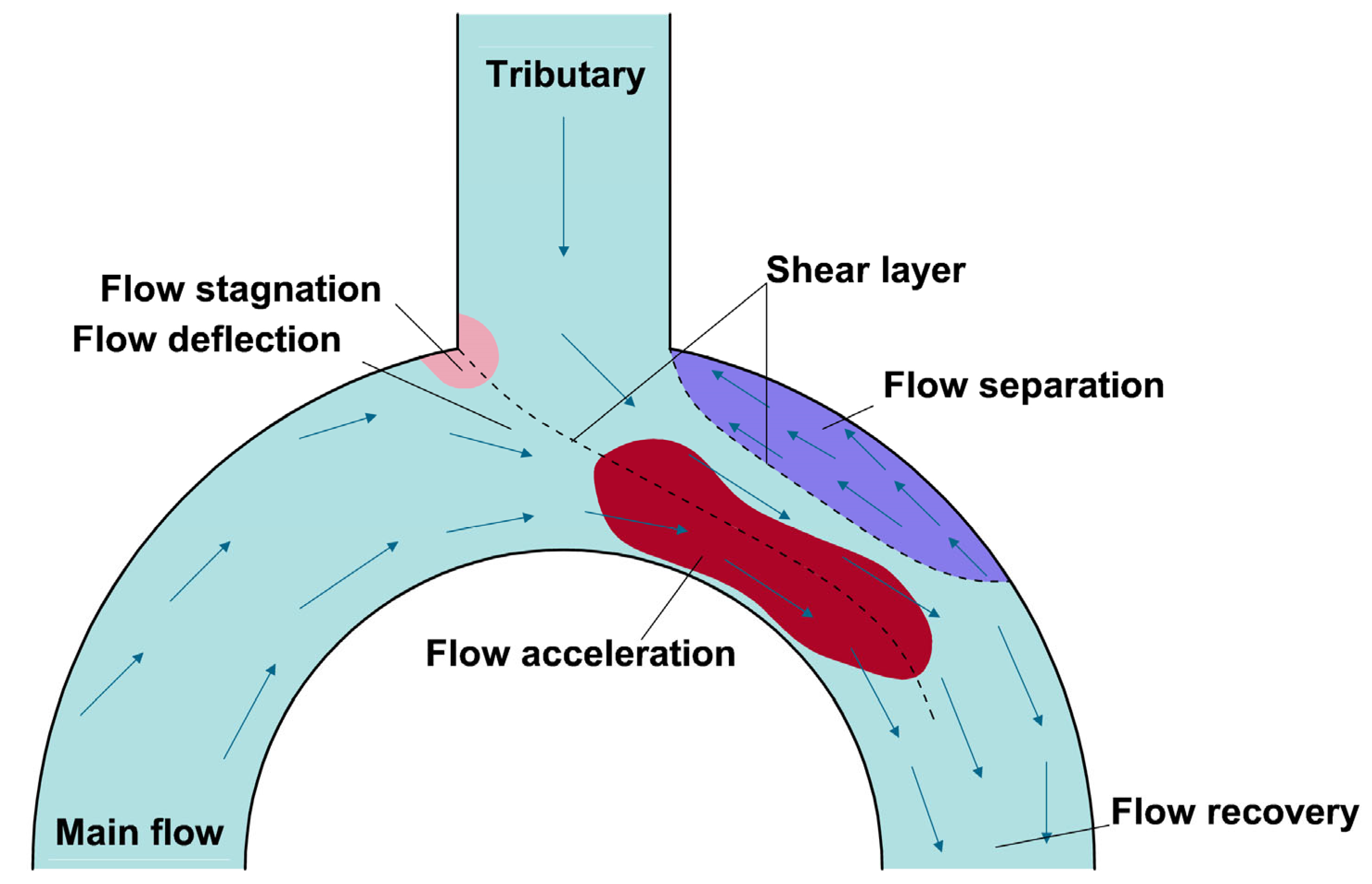
Meandering open-channel confluence flows are ubiquitous in natural and artificial rivers. Confluences play a critical role in river networks and irrigation systems. Interlaced channels form intricate flow structures in confluence areas, where strong physical gradients develop. The complex hydrodynamics further affect the local transport of pollutants and sediment, as well as aquatic vegetation seeds. According to the investigation carried out by Roberts [1], flow structures in confluence flows can be divided into six zones, which are described as stagnation zone, deflection zone, separation zone, acceleration zone, recovery zone and shear layer (shown in Figure 1). Flow velocities are much smaller in the separation zone so, there is a higher possibility that aquatic vegetation grows in separation zones. Moreover, the vegetation’s obstruction has an influence on flow structures in return resulting in a more complex hydro-environment. Due to the above, it is quite favorable for understanding flow behaviors and sedimentation issues at river confluences to study curved open-channel confluence flows with partial vegetation.
Former investigations of curved open-channel confluence flows and rigid vegetated open-channel flows are reviewed in these two paragraphs, respectively. Amounts of previous studies in confluence flows were carried out in the past two decades. Some of the studies focused on the flow behaviors and bed morphology of the natural river confluences. These studies were carried out by using different kinds of numerical models or analytical methods based on the tested data of rivers to investigate the effects between the confluence flows and bed morphology formation [2,3,4,5,6,7]. The studies took the bed discordance into consideration and found that the discordance of the bed brought the deflection to the confluence flow and changed the lateral pressure gradients resulting in the changes of secondary flow strength in the local area of confluences. Some investigations paid attention to the effects of confluence angle, flow discharge ratio and the confluence location on the flow patterns in experimental curved confluence flows [8,9,10,11,12,13]. These works gained some findings that with the increase in tributary flow discharge ratio and confluence angle the main flows were deflected more obviously towards the convex bank and the separation zone became larger in both length and width. A few researchers studied the effects of obstructions in curved confluence flows [14]. The studies mentioned above investigated the influence on open-channel confluence flows caused by bed morphology, confluence angle, and discharge ratio. Nevertheless, few of these studies took the effects of vegetation obstructions into consideration, which is a common occurrence in both natural rivers and artificial channels.
The studies of rigid vegetated flows focused on straight or curved open channels in the past twenty years. Nepf et al. [15,16,17,18,19,20] studied rigid vegetation in flow in a laboratory straight open channel to investigate the generation of shear layer caused by vegetation blockages and the turbulence in vegetated flows. As for the numerical studies, a large number of simulations were carried out in two-dimensional models by adopting shallow water equations [21,22,23,24,25]. In most 2D simulations, the effects of vegetation usually were defined as bed friction or roughness. Even though these 2D models showed the capabilities in modeling the velocity distributions of the vegetated flow, the neglect of three-dimensional effects led to the deficiency in turbulent flow and secondary flow structures. Moreover, the generalized vegetation roughness on the channel bed also resulted in an over-prediction of bed shear stress. Some investigations paid attention to the flow of vegetation in curved open channel flows and straight confluence flows [26,27,28,29,30]. These studies used the experimental method or 3-D numerical models to investigate the velocity distributions, secondary flow structures and bed shear stress of the vegetated flows. The studies demonstrated that the vegetation stems in the channel obviously compressed the flow area and pushed the secondary flow cells away from the vegetation array. In some situations, with a large density of vegetation covering the channel, the secondary flow cells were broken into small cells or even disappeared. These studies focused on meandering open channel flows with vegetation and provided analyses of the secondary flow structures. However, the flow structures in the curved open channel confluence flows are more complex than that of curved channels.
The former studies of vegetated flows focused on relatively simple flow fields with straight or curved channels. Few researchers have paid attention to the effects of vegetation on curved open channel confluence flows. Moreover, with the low velocities in the separation zone along the concave bank after the confluence, the sedimentation of silts and seeds is highly possible to occur in this area. Thus, an investigation of the effects of vegetation on separation zones, secondary flows and bed shear stress can help to understand the complex hydrodynamics in the meandering confluences and guide interests on these issues.
In this study, a numerical simulation using the VOF method and the RNG k-ε turbulence model is applied on OpenFOAM (Open Field Operation and Manipulation) to simulate the flow in a U-shaped open-channel confluence with partially emergent rigid vegetation regions near the concave bank after the confluence point. Then the hydrodynamic characteristics are analyzed in the aspect of the separation zone, water level, streamwise velocities, secondary flows and bed shear stress, to obtain the effects of rigid emergent vegetation on the flow regime of curved open-channel confluence flows.
2. Materials and Methods
In this paper, the simulation is carried out by using the incompressible multiphase flow solver interFoam [31] with the RNG k-ε turbulence model [32]. The Navier–Stokes equations in Cartesian coordinates are defined as follows:
Continuity equation
Momentum equation
where represents the fluid density, represents the velocity, represents the pressure, and are the viscous and turbulent stresses, is the component of gravitational acceleration, is the surface tension, represents the component of external forces such as the vegetation drag forces.
InterFoam solver uses the VOF method to simulate the water free-surface. In the VOF method, a volume fraction is defined to distinguish the two fluid phases in the computational domain. With the volume fraction the fluid density is defined as follows:
In this equation, is 1 when inside the fluid 1 with the density and is 0 when inside the fluid 2 with the density . The value of varies between 0 and 1 at the water free-surface. To capture the free-surface, an equation regarded as the conservation of mixture components along the path of a fluid parcel is defined for :
The surface tension in the momentum equation is also related to [33]:
where is the surface tension constant and is the curvature. The curvature is approximated as follows [34]:
The turbulence model RNG k-ε equations are shown below:
In the equations, is the turbulent kinetic energy, is the turbulence dissipation rate, is the kinematic viscosity, is the turbulence viscosity, and are the turbulent Prandtl numbers, represents the modulus of the mean rate of the strain tensor, is the strain-rate tensor, is the production of turbulence kinetic energy. The value of constant coefficients , , , , , , is shown in Table 1.
The liner central differencing scheme is used for the interpolation. The implicit Euler scheme was applied to discretize the temporal terms. The gradient terms were obtained by second order Gaussian integration. The convection terms were discretized by the van-leer scheme, a second order Total Variation Diminishing (TVD) limited scheme. The upwind scheme was employed for kinetic energy and turbulent dissipation. The PIMPLE algorithm, which is a combination of the PISO algorithm and SIMPLE algorithm, was applied for the pressure-velocity coupling at each time step iteration. The under-relaxation method was applied to reduce solution oscillations and keep the computation stable. The relaxation factor for velocities was 0.7 while it was 0.3 for the pressure, turbulence kinetic energy and turbulence dissipation rate.
As for the boundary conditions, the velocities were set based on the water flow discharges for the inflow boundary. The outflow boundary was set as a zero-gradient boundary condition. The free-surface boundary was defined as an atmospheric boundary condition. The standard wall functions were applied for the wall boundaries on the channel bed, side banks and the surfaces of the vegetation stems.
3. Model Validations and Simulation Cases Set Up
There are few available experimental investigations on curved open channel confluence flow with rigid vegetation, in this chapter, an experiment of a U-shape open channel flow through partially rigid vegetation and another hydraulic experiment in the same U-shape open channel with a tributary were chosen to be simulated to complete the validation.
3.1. Curved Open Channel Flow with Partially Rigid Vegetation
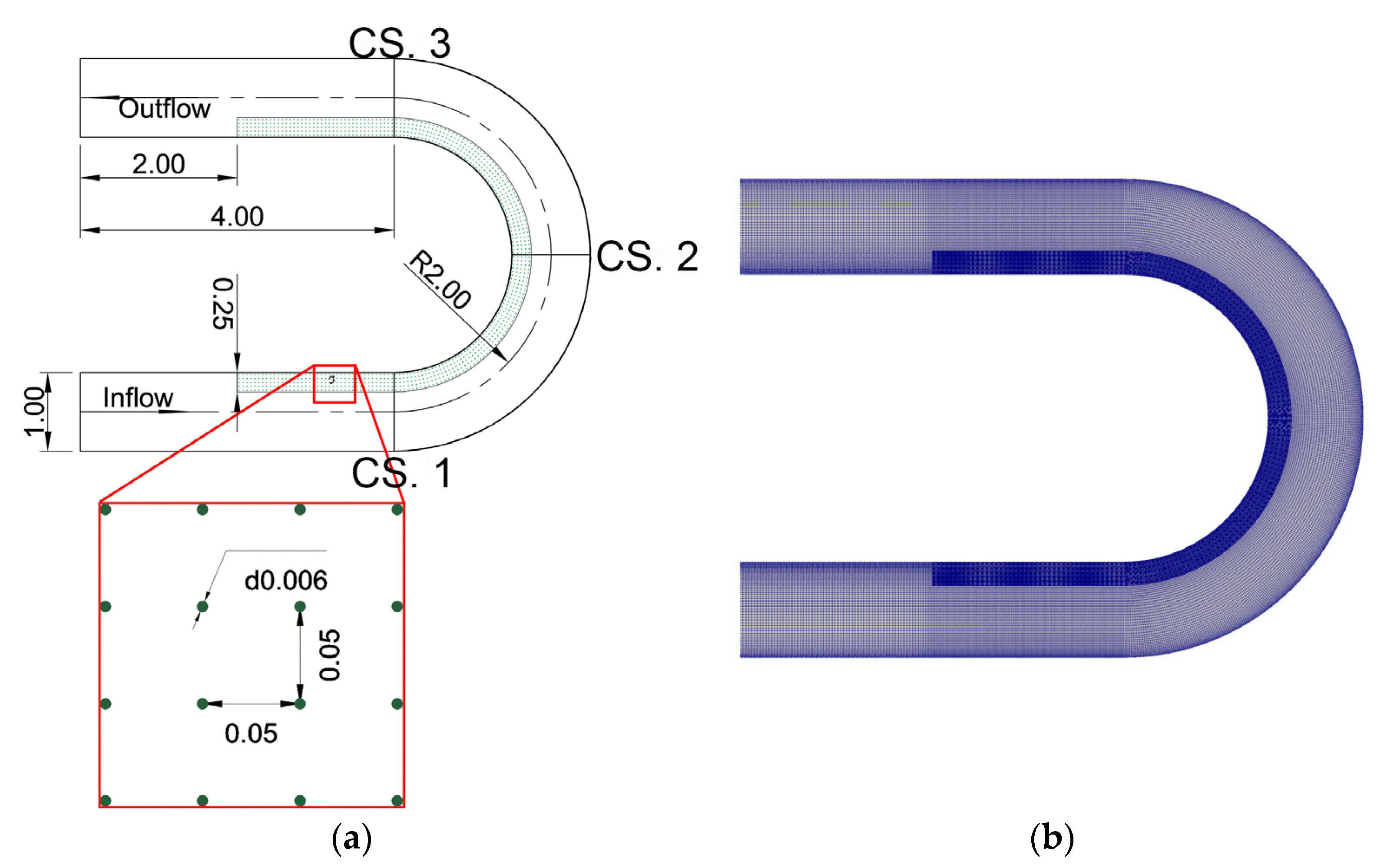
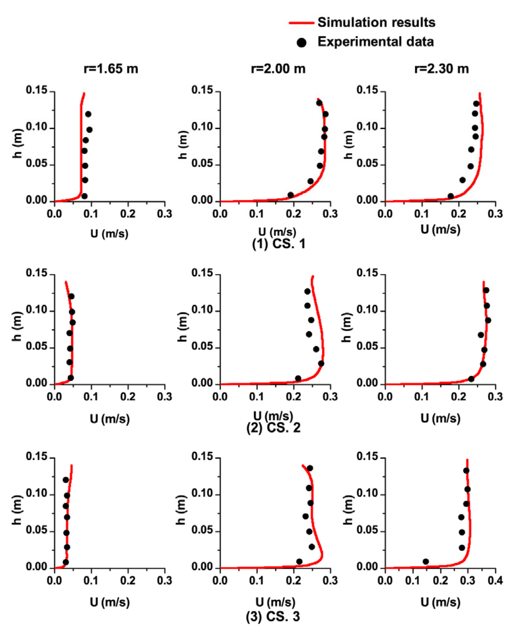
The experiment of a U-shaped open-channel flow through partially rigid vegetation was carried out by Huai et al. [27] at the State Key Laboratory of Water Resources and Hydropower Engineering Science, Wuhan University, Wuhan, China. The experimental flume with a 1 m wide and 0.25 m high rectangular cross-section consisted of a 4 m straight inflow reach, a 180° curved reach, and a 4 m straight outflow reach. The radius R of the centerline in the curved reach was 2 m. A 0.25 m wide band was placed along the convex bank from 2 m after the inlet to 2 m before the outlet. To simulate the rigid vegetation, reinforcing steel bars with 0.006 m diameter were perpendicularly planted on the band with a 0.05 m interval space. The height of the steel bars was 0.15 m. The water permeability of stems was neglected. The inflow discharge was 0.03 m3/s and the water depth measured at the outlet was 0.148 m. The sketch of this experiment is shown in Figure 2a. The mean streamwise velocity profiles of test lines (r=1.65 m, 2.00 m, and 2.30 m, respectively) on the three chosen test cross sections (the entrance, middle and exit of the curved reach) were sampled to compare with the experimental data.
The calculating mesh was created by the commercial software ICEM-CFD. According to a mesh in-dependency analysis, a structured 6.94-million-cell mesh was determined with local refinement in the vegetation region on the convex bank (shown in Figure 2b). The minimum mesh size was 0.0015 m for the first layer of mesh at the wall boundaries of the surface on vegetation stems. This was to keep the y-plus value within an appropriate range () to ensure the effectiveness of the standard wall function method. The boundary conditions were the same as those described in Section 2. The volume fraction of the part below the water level in the computational domain was set to 1 for the initialization of the calculation. The time step was controlled at 0.00175 s so that the Courant number was kept below 1.
The comparison of the mean streamwise velocity profiles on the test lines of the three cross-sections between the experimental data and simulation results is shown in Figure 3. The simulation results were basically consistent with the experimental data. Figure 4 shows the comparison of secondary flow structures on the test cross-sections between experimental data and simulation results. The secondary flow structures of the simulation results were similar to those of the experimental data.
To evaluate the agreement between the simulation results and the experiment data, the indexes root-mean-squared error (RMSE) and coefficient of determination () were calculated on the three tested cross-sections. The formulas of RMSE and are described as below:
where represents the number of values in the experiment data, is the measured value, is the calculated value, and represents the average value of . The RMSE value can show the dispersion degree of the data. A smaller RMSE value indicates a better prediction of the model. Moreover, the value is a quantized form for the goodness of fit. The value of is usually between 0 and 1, a better fit is gained when the value is closer to 1. Table 2 shows the sectional RMSE and of mean streamwise velocities.
The RMSE values on the three tested cross-sections were quite small and the values of were close to 1, which indicated the reliability of the model in predicting the mean streamwise velocities. Especially, the RMSE value of CS. 2 was smaller and the value was larger, which means that the model was better in the curved reach than at the entrance and exit of the curved reach. This was similar to the results gained by Shaheed et al. in modeling a curved open channel flow by using k-ε models. Basically, the validation demonstrated the capability of the numerical model in simulating flows in curved open channels with partially rigid vegetation.
3.2. Curved Open Channel Confluence Flow
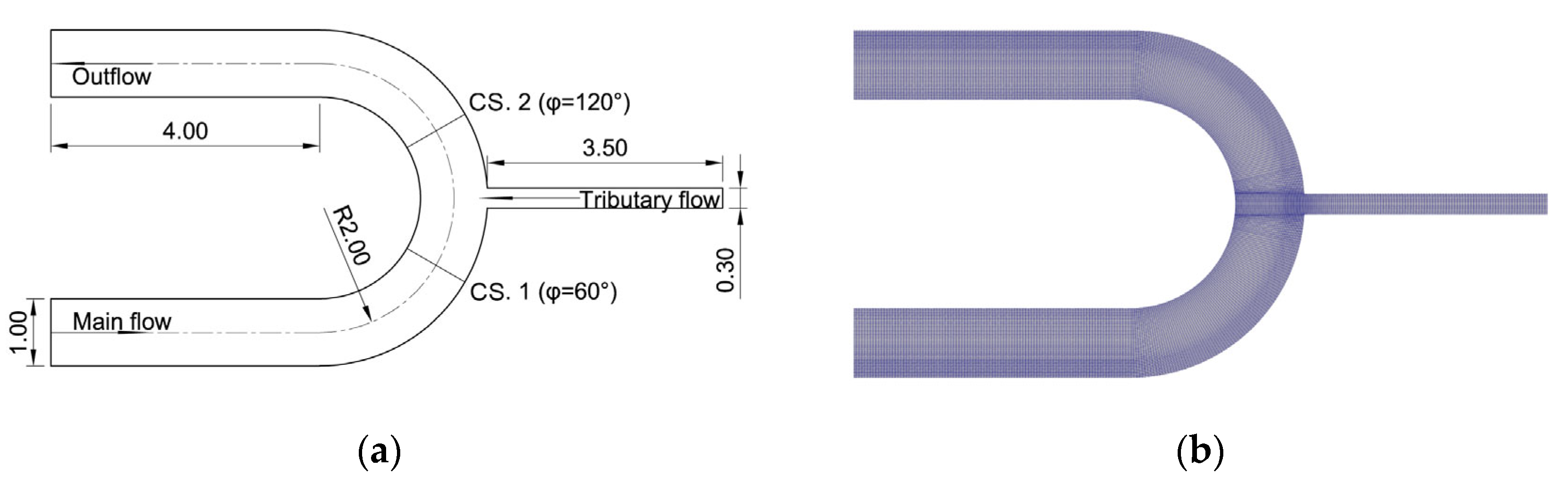
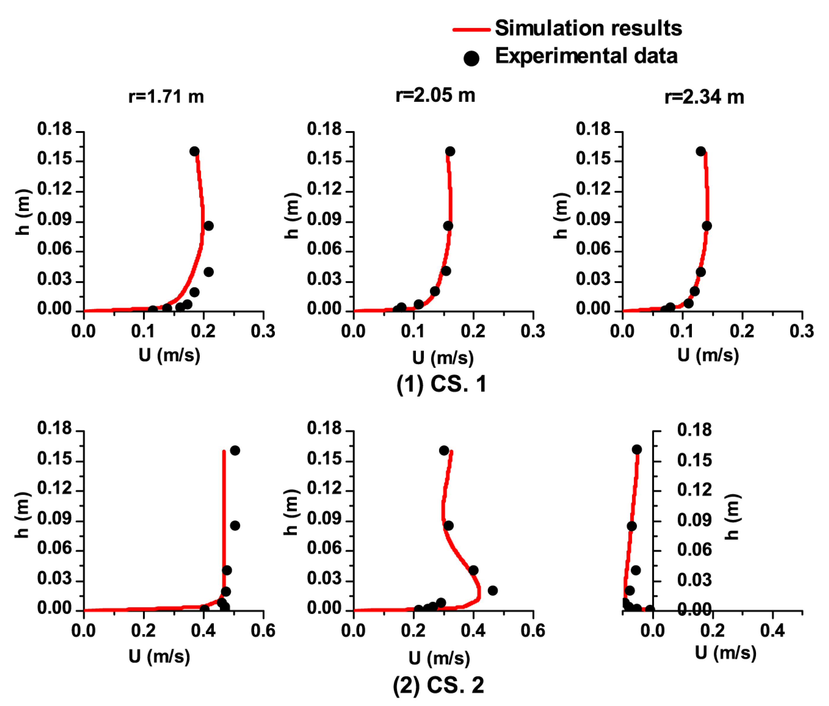
The physical modeling investigation of a curved open channel confluence flow was performed by Sui et al. [12]. The main channel was the same as the U-shaped channel described above in Section 3.1. The tributary channel was a 3.5 m-long straight flume with a 0.3 m wide and 0.25 m high rectangular cross-section. The confluence was located at a 90° cross-section of the curved reach and the confluence angle between the tributary and the main channel was also 90°. As for the hydraulic conditions, the main channel inflow discharge was 0.03 m3/s and the tributary discharge was 0.018 m3/s. The water level measured at the entrance of the curved reach was 0.182 m. Test lines (r = 1.71 m, 2.05 m, and 2.34 m, respectively) on the two cross sections (CS. 1 φ = 60° and CS. 2 φ = 120°) were chosen to validate the experimental data. The schematic of the experiment is shown in Figure 5a.
The calculating mesh owned 1.15 million structured cells with local refinement at the confluence point (shown in Figure 5b). The minimum mesh size was 0.003 m for the first layer of mesh at the wall boundaries. The volume fraction of the part below the water level in the computational domain was set to 1 for the initialization of the calculation. The time step was controlled at 0.0123 s to keep the Courant number no more than 1.
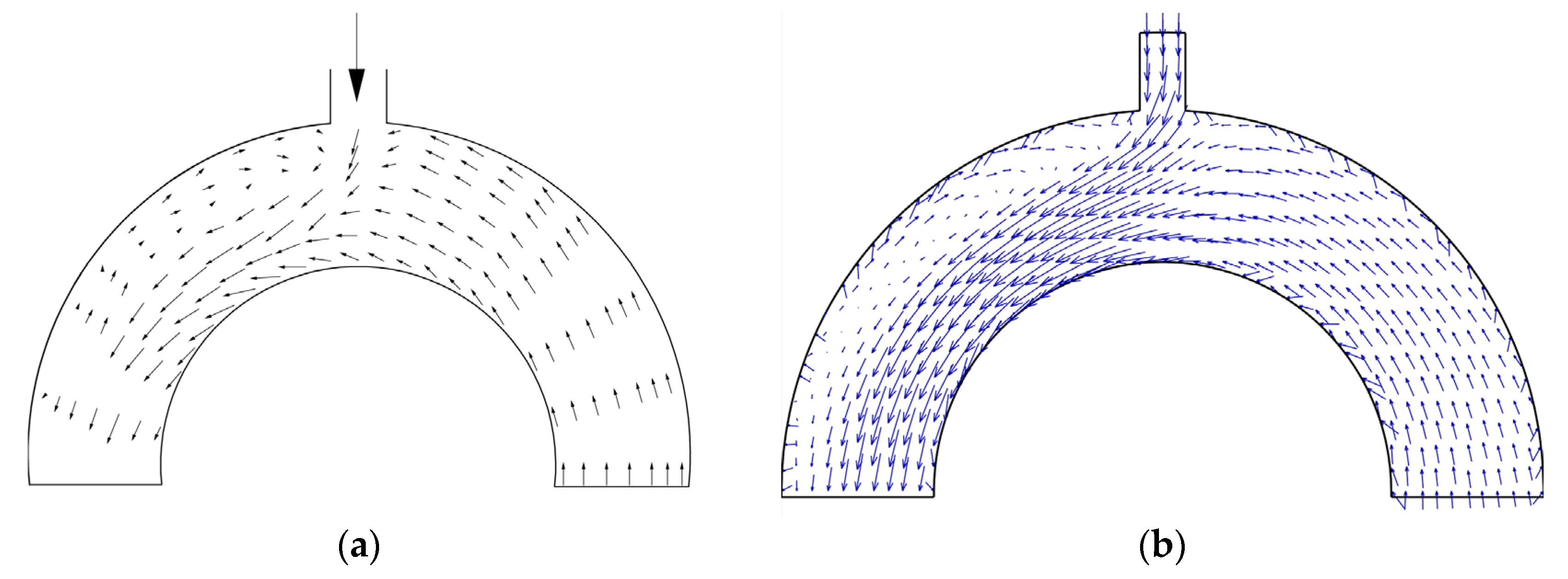
The comparison of the mean streamwise velocity profiles on the test lines of the two cross-sections between the experimental data and simulation results is shown in Figure 6. Good agreements were obtained. Table 3 shows the RMSE and values on the two tested cross-sections. The reliability of the model was proved. Figure 7 displays the comparison of free-surface velocity vectors between experimental data and simulation results. The simulation results showed the same trends for the velocity vectors as the experimental data. The comparison of results confirmed the ability of the numerical model to simulate confluence flows in curved open channels with a separation zone.
3.3. Numerical Simulation Cases Set Up
Based on the numerical model validations above, the capability of the model to simulate the curved open channel confluence flows through rigid vegetation was verified. Then the model was adopted to study the effects of partially emergent rigid vegetation on a U-shaped open-channel confluence flow.
Based on the validation simulations above, the numerical simulations were carried out in the same U-shaped channel as in the experiment described in Section 3.2. Likewise, the main channel inflow discharge and water level were also the same as the second validation case. This was for controlling variables so as to compare the results with different tributary flow discharge ratios. Then two different discharge ratios (, represents the tributary flow discharge) were chosen in the simulations. As for the vegetated cases, considering the higher possibility of vegetation growing in the low velocities zone along the concave bank, a 0.25 m-wide vegetation region was set along the concave bank after the confluence point. The vegetation stems with no water permeability considered were all 0.25 m height to keep the stems sticking out of the water free-surface. The stems were arranged in parallel. Two different stem diameters and interval spaces were set in different cases. Three cross-sections (CS. 1: the cross-section right before the confluence point; CS. 2: the 135° cross-section of the curved reach; CS. 3: the exitance section of the curved reach) in the main channel were monitored. The mesh used in simulations had about 3.68 million structured grids with local refinement along the concave bank after the confluence point. The minimum size of the grid near the wall boundary was also 0.0015 m. The computing time step was set to be about 0.00175 s. The details of all the cases are shown in Table 4. The simulation schematic and the calculating mesh are shown in Figure 8.
4. Results and Discussion
In this section, the flow analysis was performed from the following aspects of streamwise velocities, separation zone, water level, cross-section secondary flows, bed shear stress and flow resistance.
4.1. Steam-Wise Velocities and Separation Zone
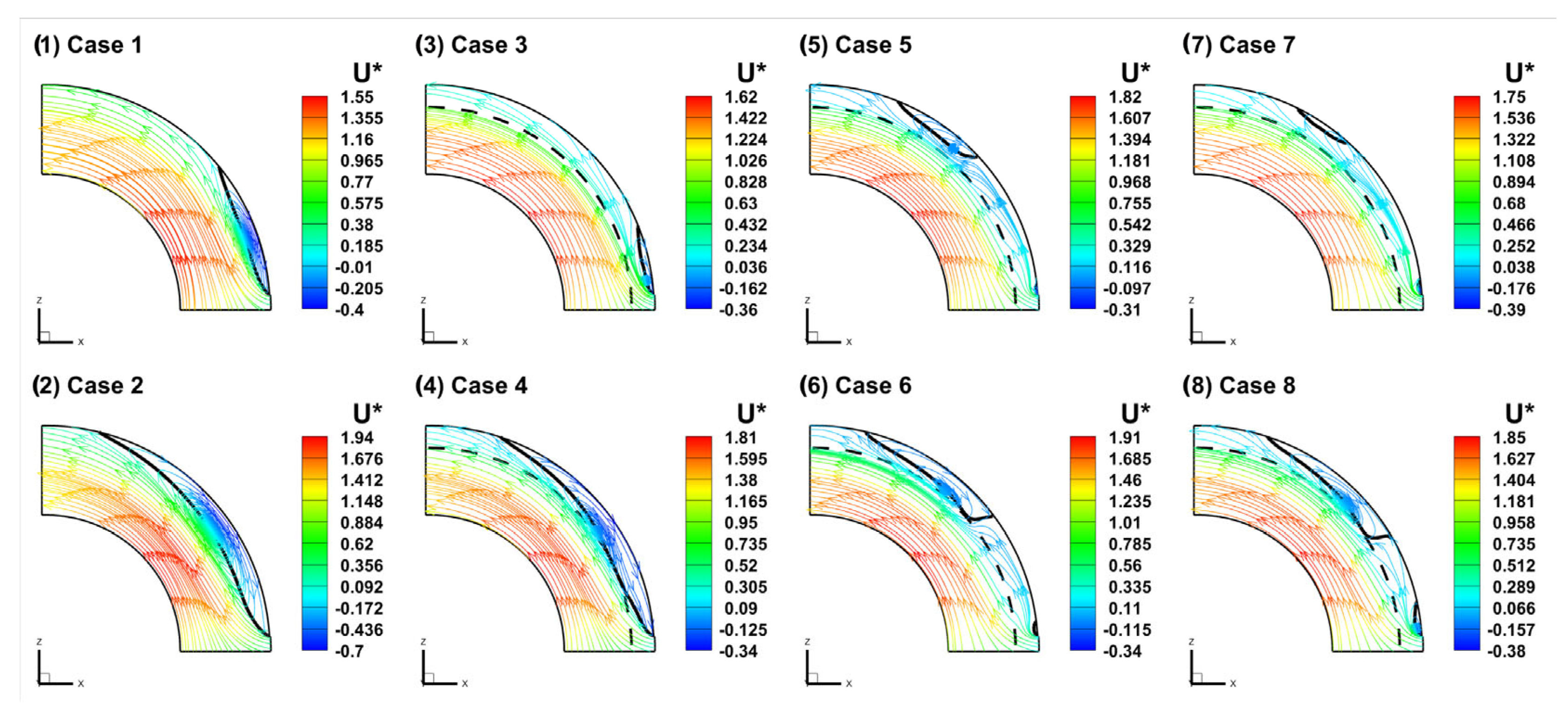
Figure 9 below displays the contours and 2-D streamlines of dimensionless streamwise velocities (, represents the averaged velocity on the cross-section along the curved channel) on the vertical section near the water surface in the curved reach after the confluence point of all the cases. In the non-vegetated cases, the velocities on the convex bank were significantly greater than those on the concave bank, and the velocity difference between the convex bank and concave bank increased with the increase in tributary discharge. Because the tributary flow on the concave bank brought a lateral impact to the main flow and deflected the main flow to the convex bank after the confluence point. A strong shear layer with a large velocity gradient and momentum exchange was generated. So, a larger tributary discharge caused a much stronger flow deflection and resulted in a larger velocity difference between the convex bank and the concave bank. Moreover, the strong shear layer divided the main flow into two parts, a separation zone with smaller reversed velocities near the concave bank and a flow acceleration zone with the largest velocities near the convex bank, respectively. Thus, the border of the separation zone could be obtained by sampling the points with zero streamwise velocities. In Figure 9, the black solid lines represent the sampled separation borders and the dashed lines represent the edge of the vegetation region in vegetated cases. From the streamlines in Case 1 and Case 2, a circulation was formed beside the concave bank after the confluence point. The circulation extended in both length and width as the tributary discharge increased. Moreover, the border of the separation zone just passed through the center of circulation. The size of the separation zone also increased in both length and width with the increase in tributary flow discharge. As for the vegetated cases, the flow velocities decreased obviously in the vegetation region due to the vegetation blockage. With higher Solid Volume Fraction (SVF), the velocities in the vegetation region decreased more obviously. The circulations were also much smaller than those in the non-vegetated cases and the separation zones became smaller in length and width as well. Especially, in the cases with higher SVF, the position of the separation zone was different from the cases with low SVF. In Cases 1–4, there was only one large separation zone located right after the confluence point. However, in Cases 5–8, a relatively smaller separation zone was located at the channel confluence while another large separation zone was captured near the downstream of the curved channel. According to the 2-D streamlines, the streamlines near the concave bank became disordered as the vegetation resistance increased. In cases 1–4, with smaller resistance, the tributary flow rushed into the main channel and formed a circulation after the confluence point. While in cases 5–8, the tributary flow was disturbed by the large resistance and divided into two parts. A little part whirled at the corner right after the confluence point forming the little separation zone and the other part flowed through the stem space and slowed down gradually downstream which formed the large separation. Moreover, it could be observed that in the non-vegetated cases the main flow streamlines deflected in a similar direction to the separation zone extensions. However, in the vegetated cases the main flow streamlines deflected along the edge of the vegetation region.
Figure 10 shows the contours of the radial gradient of streamwise velocities on the vertical section near the water surface in the curved reach after the confluence point. It is obvious that a shear layer with a large negative velocity gradient was formed between the midline and concave bank. In the shear layer, the velocities changed fast and the momentum exchange was violent. In the non-vegetated cases, the shear layer was located right beside the border of the separation zone. With the tributary discharge increased, the value of the velocity gradient increased and the range of the shear layer became larger. In the vegetated cases, due to the blockage of stems, the velocity gradient in the vegetation region was relatively small. The shear layer is located beside the edge of the vegetation region and deflected slightly towards the midline. This phenomenon is consistent with the deflection of streamlines in Figure 9. What is more, the velocity gradient at the beginning of the vegetation region was quite large. This is because the tributary flow with large velocities knocked into the vegetation stems generating a sharp decline in velocities.
4.2. Water Level
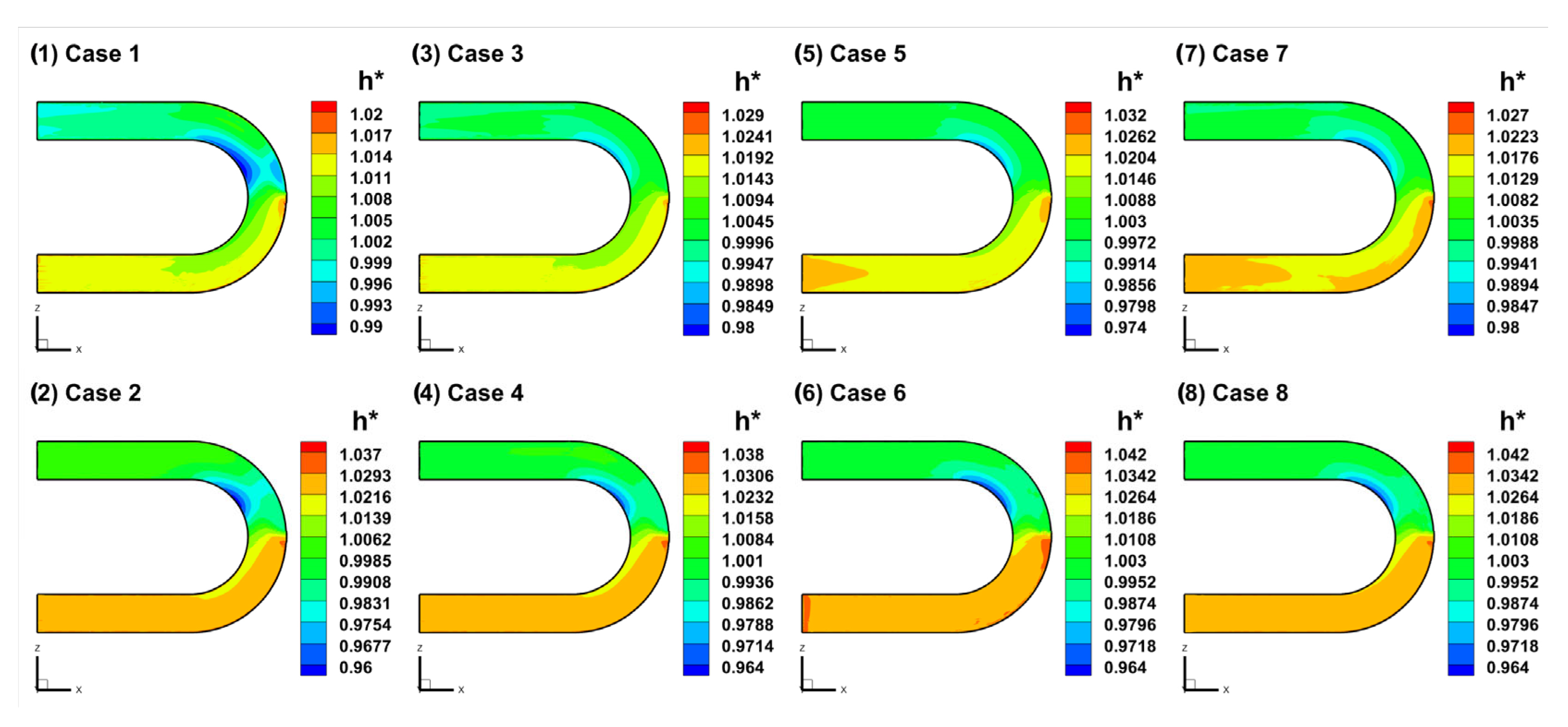
Figure 11 below shows the dimensionless water level () contours in the main channel of all the cases. According to the water level contours, for all the cases, the lowest water level is located near the convex bank in the curved reach after the confluence point due to the centrifugal force. This character is basically consistent with that in curved open channel flow. In the non-vegetated cases, the water level near the concave bank in the separation zone fell visibly as the tributary discharge ratio increased. That is because the tributary flow diverted water from the concave bank into the central channel. As the tributary discharge increased, backwater occurred upstream of the confluence, which caused the water level to increase sharply; the waterhead before and after the confluence was much larger. The lowest water level points also moved downstream as the tributary discharge increased. For the vegetated cases, the water level at the confluence point rose due to the blockage of the vegetation. The downstream water level varied obviously along the channel width near the convex bank while the water level of the concave bank became relatively flat. The low water level area near the convex bank shrunk compared to that in the non-vegetated case because the vegetation region blocked the flows and narrowed the main flow area. With the increase in SVF, the upstream water level became higher and the waterhead between upstream and downstream became larger. Especially with the same SVF (), the upstream water level in Case 5 was a little bit higher than that in Case 7, and a similar result was also found between Case 6 and Case 8. This phenomenon demonstrates that under the same solid volume fraction and water barrier area a larger vegetation density brings more resistance to the flow than a larger stem diameter.
4.3. Cross-Section Secondary Flow
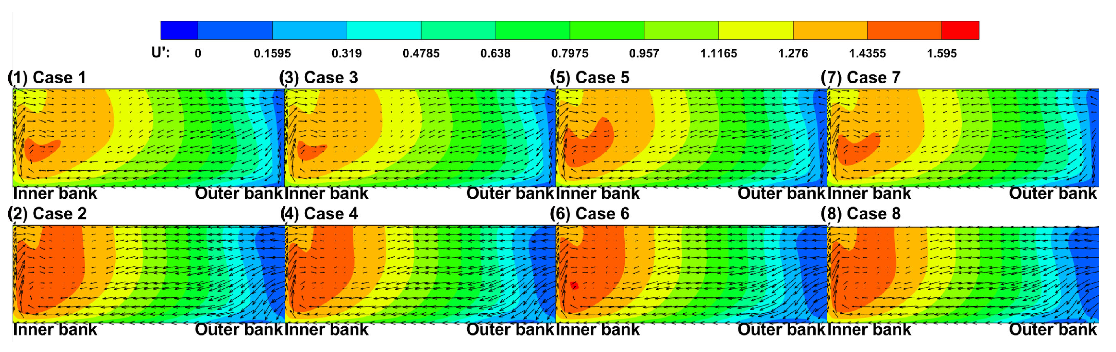
To totally study the effects of discharge ratios and vegetation on secondary flow structures, three typical cross-sections were chosen. The three cross-sections were the upstream cross-section right before the confluence point, the 135° intersecting surface in the curved reach and the exit section of the channel bend, respectively (shown in Figure 8a).
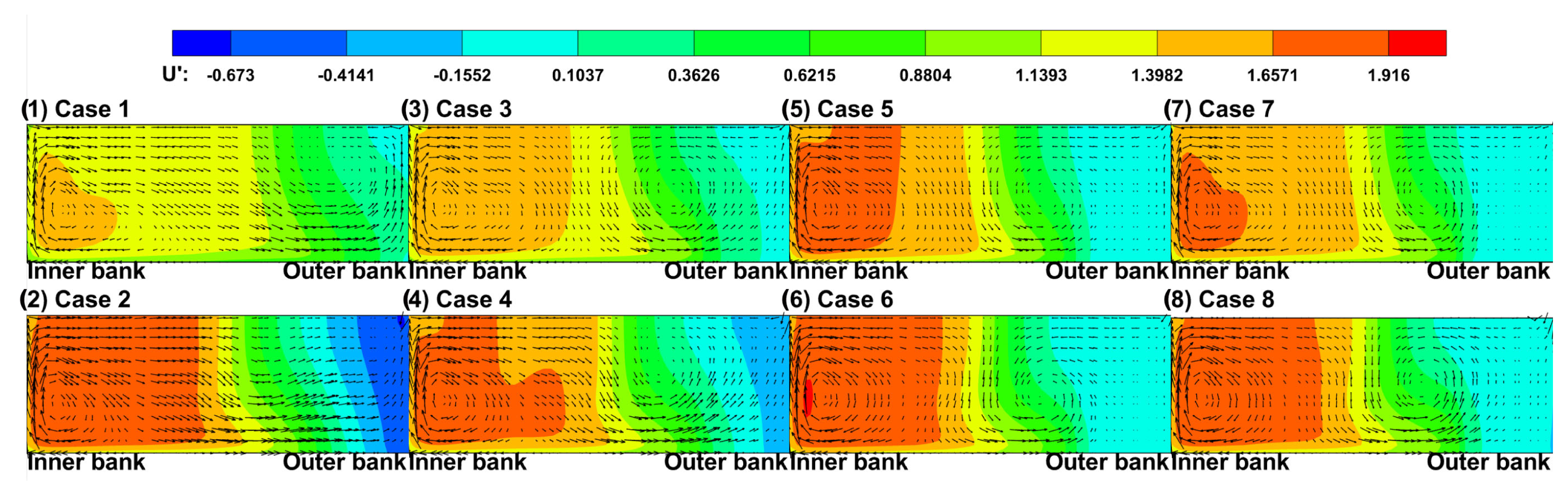
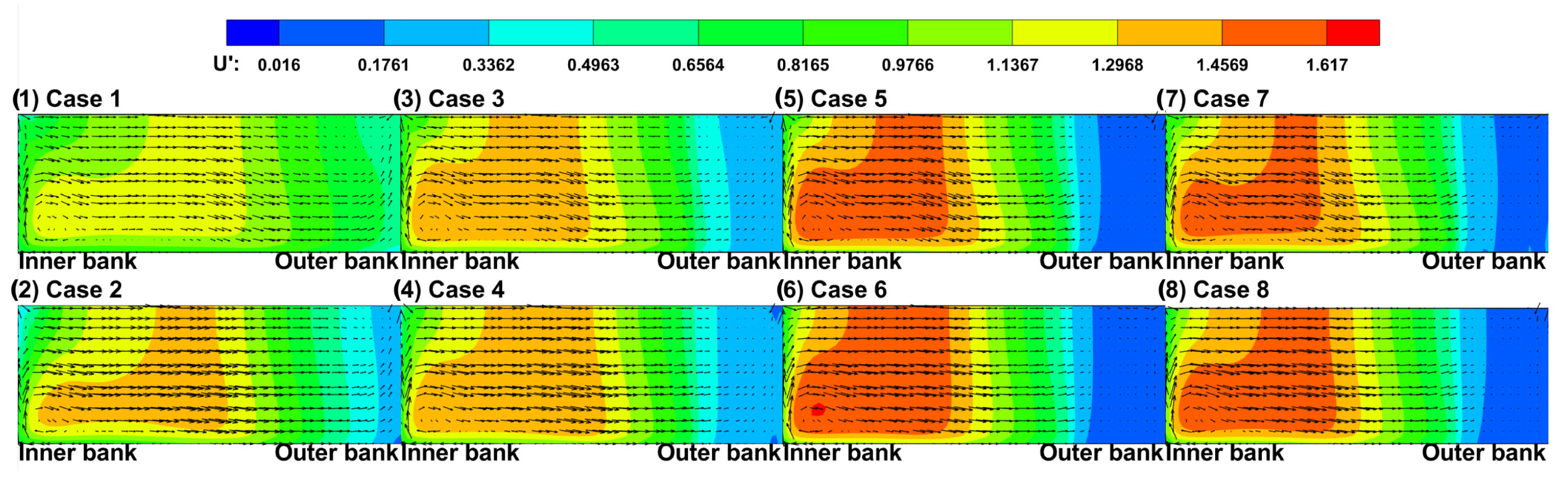
Figure 12, Figure 13 and Figure 14 below exhibit the contours of dimensionless streamwise velocity (, represents the averaged velocity in the cross-section) distribution and 2-D velocity vectors on the three cross-sections of all the cases. According to the velocity contours, the maximum streamwise velocity occurred near the convex bank, which was consistent with Figure 9. On the upstream cross-section of the confluence point, with the tributary discharge ratio increased, the maximum velocity regions moved close to the convex bank. The dimensionless velocity near the convex bank increased while on the concave bank the dimensionless velocity decreased. There were only minor changes in velocity distribution between vegetated cases and non-vegetated cases on CS. 1, which demonstrated that the vegetation region after the confluence point had less influence on the upstream cross-section than the tributary flows. In CS. 2 and CS. 3, the dimensionless velocity on the concave bank became obviously much smaller in the vegetated cases, the minimum velocity region basically overlapped with the vegetation region. From the velocity vectors on the cross-sections, due to the centrifugal force, a clockwise main circulation cell was located near the channel bed of the convex bank, which was in tune with the curved open channel flow. As the tributary discharge and vegetation SVF increased, the scope of main circulation cells apparently shrunk. On the upstream cross-section right before the confluence point, due to the tributary flow, there was no circulation cell on the concave bank. In CS. 2, besides the main circulation cell, there was another reversed smaller circulation on the concave bank. The concave bank circulation was formed by the effects of turbulence flow and the driving forces brought by the main circulation cell. In the vegetated cases, the main circulation cell near the convex bank shrunk and the concave-bank circulation moved towards the channel midline. This phenomenon was much more apparent in the cases with higher SVF. Moreover, in the vegetation region, due to the obstruction of stems, the anisotropy of turbulence flow was enhanced so that the vectors became smaller and more chaotic. Moreover, in CS. 3, the main circulation cells near the bed of the convex bank were much smaller than those in CS. 1 and CS. 2. The circulations near the concave bank also shrunk significantly, which in the vegetated cases were hardly observed.
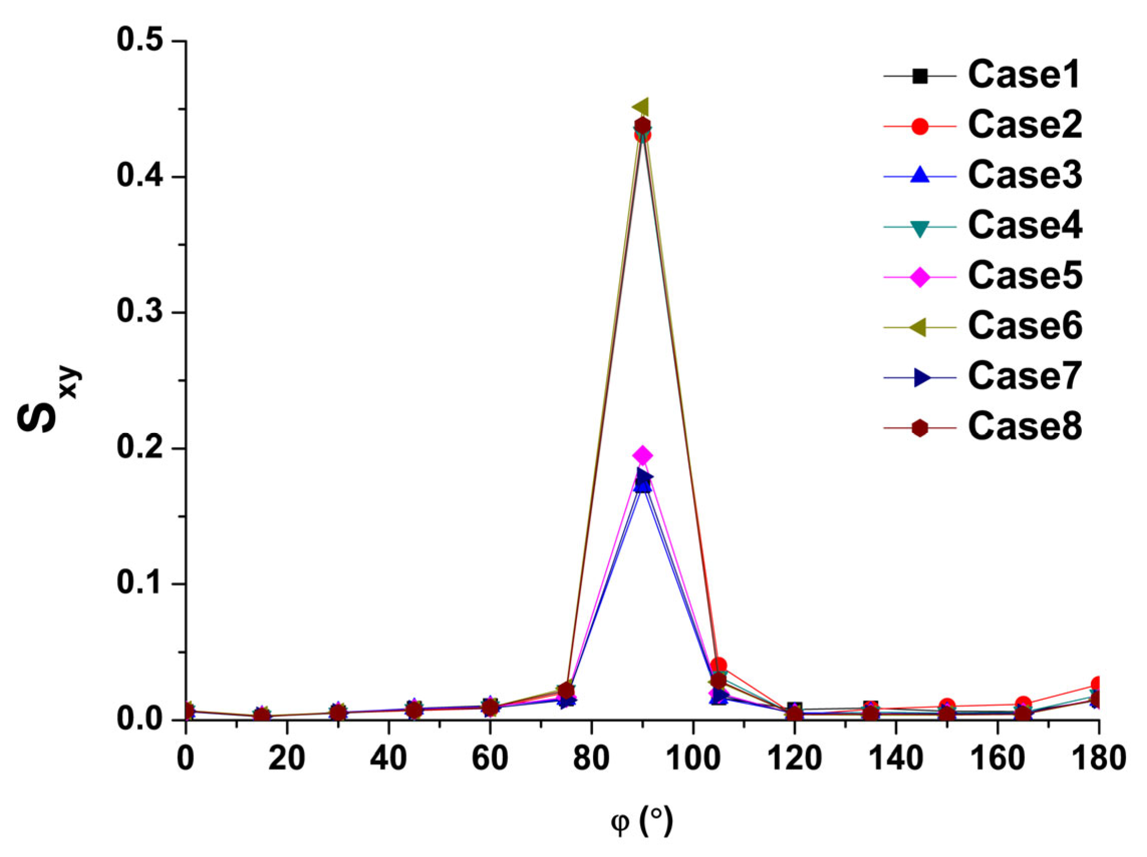
The secondary flow strength is described by a dimensionless coefficient , which was introduced by Shukry [35] in his studies on the streamflow at the riverbank. The coefficient represents the kinetic energy ratio of the lateral current and mainstream on a given cross-section, and the formula is defined as follows:
where , and represents the streamwise velocity, radial velocity and vertical velocity on the cross-section, respectively.
Figure 15 shows the secondary flow strength on the cross-sections along the curved reach of all the cases. According to the lines, the secondary flow strength before the confluence point increased gradually along the channel and was almost the same in all the cases with different flow discharge ratios and different vegetation densities. This phenomenon demonstrates the tributary and vegetation had a tiny effect on the upstream secondary flows which increased due to the centrifugal effects brought by the curvature. The largest point is located at the 90° cross-section with a sharp increase around the confluence point. This is because the tributary flow brought a strong lateral current to the main flow and the turbulence characteristics were strengthened in the confluence area. Moreover, in the cases with a larger tributary discharge ratio ( the maximum secondary flow strength was much larger than those in the cases with a smaller discharge ratio (. After the confluence point, the secondary flow strength declined dramatically and reached the minimum value at the 120° cross-section. That is because the flow acceleration zone with the narrowest main flow width was located in this area and the streamwise velocities reached the maximum value. The kinetic energy of the mainstream was much larger than the that of lateral current. After the 120° cross-section, in the non-vegetated cases, the secondary flow strength increased gradually along the channel. While in the vegetated cases, due to the blockage brought by the vegetation, the width of the main flow was narrowed along the channel and the secondary flow strength hardly changed until the 180° cross-section. What is more, as the vegetation resistance blocked the flow on the concave bank, the secondary strength in the vegetated cases was larger at the 90° cross-section and smaller in the downstream curved reach than that in the non-vegetated cases.
4.4. Bed Shear Stress
The dimensionless bed shear stress, i.e., friction coefficient can be defined as the following expression:
where represents the bed shear stress, represents the water density, and represents the averaged streamwise velocity at the channel exit.
Figure 16 displays the contours of bed shear stress friction coefficient of the main channel in all the cases. According to the investigation carried out by Kashyap et al. [36], for the high curvature flatbed channels (), the region of maximum bed shear stress is located near the convex bank upstream after the curved reach entrance, and gradually moves towards the concave bank downstream. While in this paper, the results were quite different from those in curved open channels. The region of maximum bed shear stress was always located near the convex bank along the whole curved reach. The tributary flow deflected the main flow from the concave bank to the convex bank and induced a large velocity difference between the inner side and outer side of the curved channel. The near-bed vertical velocity gradient was much larger on the convex bank than that on the concave bank. As the same as the streamwise velocities, with the increase in tributary discharge, the difference in bed shear stress between the convex and concave banks was obviously larger. For vegetated cases, due to the resistance brought by stems, the velocities near the convex bank became much larger, and so was the near-bed velocity gradient. Then the bed shear stress in the non-vegetated region was also much larger than in the vegetation region. With the increase in SVF, the maximum bed shear stress became larger. Especially, with the same SVF (), the maximum bed shear stress in Case 5 and Case 6 was a little bit bigger than that in Case 7 and Case 8. The reason leading to these results is similar to the streamwise velocity gradient. The bed shear stress is in proportion to the near-bed vertical velocity gradient [37]. Moreover, in the non-vegetated cases, the maximum bed shear stress near the convex bank basically occurred in the flow acceleration zone which was on the opposite of the separation zone. While in the vegetated cases, the maximum bed shear stress region almost covered the convex bank after the confluence point. Furthermore, near the concave bank, there was a dramatic decline in the friction coefficient. Moreover, in the non-vegetated cases, the region of decline was associated with the tributary discharge, with the increase in tributary discharge, the decline region moved gradually from the concave bank to the midline. While in the vegetated cases, the dramatic decline of bed shear stress basically occurred around the edge of the vegetation region.
4.5. Flow Resistance
The flow resistance brought by rigid vegetation is often quantified by the vegetation drag coefficient, which is a normalized form of drag force. The drag coefficient of a single vegetation stem is defined below:
where represents the drag force of the stem, is the projection area of the stem, is the fluid density, is the reference velocity approach to the stem. Since the velocity approach to a stem is quite difficult to observe in a vegetation array, the drag coefficient of the stem is also defined as an averaged drag coefficient:
where represents the total drag force of the vegetation array, is the projection area of the stem, is the fluid density, is the number of stems in the array, and is the averaged streamwise velocity on the cross-section right before the vegetation region.
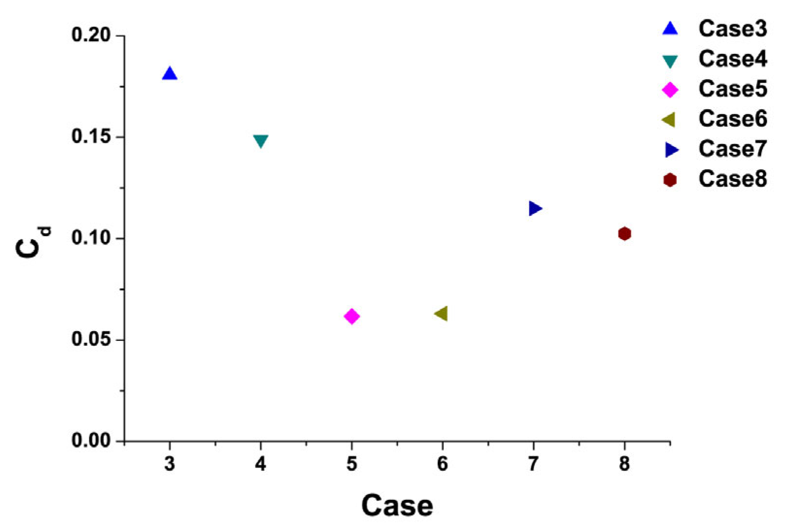
The time-averaged drag coefficients of all the vegetated cases are shown in Figure 17 below. According to Figure 17, the drag coefficients of all the cases were quite small due to the low velocities on the concave bank after the curved open channel confluence. The low velocities in the separation zone brought weak interaction between the flow and stems, and the drag forces in this area were very small. Comparing the drag coefficients in the cases, with the same planting scheme, the drag coefficients in the cases with larger flow discharge were a bit smaller than those in the cases with smaller discharge. Moreover, the drag coefficients decreased obviously with the increase in SVF. Under the same SVF (), the drag coefficients in Case 5 and Case 6 were much smaller than those in Case 7 and Case 8. The results indicate that the vegetation drag coefficient in the curved open channel confluence flow decreases with the increase in stem Reynolds number and vegetation planting density, which is consistent with the findings in Tanino and Nepf [38].
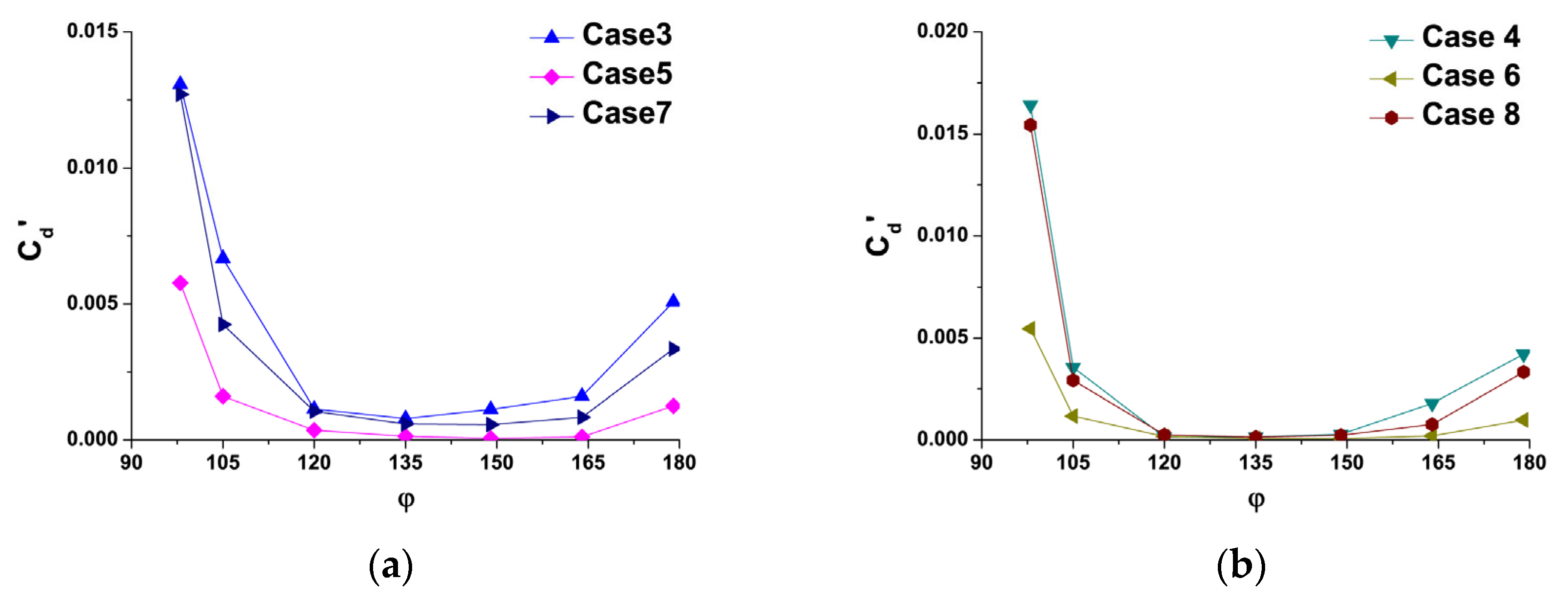
Figure 18a,b display the local time-averaged drag coefficients along the curved channel after the confluence. From Figure 18, in each case, the local drag coefficients showed the same variation trend. The largest drag coefficient occurred at the beginning of the vegetation array. The large flow velocities coming from the confluence point knocked into the vegetation with a strong impact. In the middle reach of the vegetation zone, the flow was deflected to the convex bank; the velocities in this area were relatively smaller, thus the smallest drag coefficient located in this area. With the flow recovery before the exit of the curved reach, the drag coefficient became a little bit larger. Comparing the drag coefficients in the cases with the two different discharge ratios, the drag coefficients in the cases with larger tributary discharge were larger at the beginning of the vegetation array and smaller downstream of the confluence. This was because the larger tributary discharge brought a stronger impact to the stems at the beginning of the vegetation region and deflected the main flow downstream more obviously away from the concave bank towards the convex bank.
5. Conclusions
The hydrodynamics of a U-shape open channel confluence flow with partially rigid emergent vegetation were simulated by the RNG k-ε numerical model coupled with the VOF method in OpenFOAM. The results of streamwise velocity, separation zone, water level, cross-section secondary flows and bed shear stress were analyzed. Some main findings are summarized as follows:
- The streamwise velocities of the convex bank were significantly greater than those of the concave bank and this velocity difference increased as the tributary discharge increased. The vegetation blocked the tributary flow to the mainstream causing an obvious decrease in velocities in the vegetation region. Moreover, the velocity difference between the convex bank and the concave bank was much larger. This change was more apparent with the higher vegetation solid volume fraction.
- The tributary flow impacted and deflected the main flow producing a separation zone with reversed smaller velocities on the concave bank after the confluence point. With the increase in tributary discharge, the separation zone became larger in both length and width. The vegetation near the concave bank played a role in blockage on the tributary flow and changed the mainstream deflecting direction. Compared to the non-vegetated cases, the separation zone was much smaller in length and width. Especially, with higher vegetation solid volume fraction (), the separation zone was divided into two parts, a smaller one right after the confluence point and a larger one on the second half of the curved reach after the confluence.
- The lowest water level point was located near the convex bank in the curved reach after the confluence point. Moreover, with the tributary discharge increased, the water level before the confluence increased while the water level after the confluence fell visibly. The lowest water level points also moved downstream as the tributary discharge increased. The vegetation brought resistance to the tributary flow causing backwater upstream of the confluence. The water level varied fast near the convex bank and tended to be gentle in the channel midline. With the same SVF (), a larger vegetation density brought more resistance to the tributary flow than a larger vegetation stem diameter.
- On the upstream cross-section right before the confluence point, there was only one main circulation cell located near the channel bed of the convex bank. While on the downstream cross-sections, besides the main circulation cell, there was another reversed smaller circulation on the concave bank. As the tributary discharge and vegetation SVF increased, the main circulation cell apparently shrunk and the concave-bank circulation moved towards the channel midline. Moreover, on the 180° cross-section, the circulation cells were much smaller than those in the curved reach. The maximum secondary flow strength was at the 90° cross-section where the confluence point was located.
- As the same trends of streamwise velocities, the region of maximum bed shear stress was always located near the convex bank along the whole curved reach. Compared to the non-vegetated case, the maximum bed shear stress was much larger in the vegetated case. Moreover, the bed shear stress in the non-vegetated region was also larger than that in the vegetated region. As the vegetation SVF increased, this difference became larger.
- The time-averaged drag coefficients of the vegetation decreased with the increase in stem Reynolds number and vegetation planting density. Along the arc length of the vegetation region, the largest local drag coefficient was located at the beginning of the region and decreased sharply in the middle reach, then it became a little bit larger downstream before the exit of the curved reach.
In this study, a U-shape open channel flow with a tributary on the concave bank was simulated by a numerical model. An emergent rigid vegetation region was set on the concave bank after the confluence point. The effects of tributary discharge ratio and vegetation density on the hydrodynamics were analyzed based on the results. This work provided a reference guide to understanding the dynamics and structures of the weedy interlaced meandering channels. The main implications of the study are to benefit water ecological management and restoration, whether natural rivers or urban artificial canals.
However, there are still lots of problems that are worthy of being investigated in this issue. In this study, the open channel was a 180° curved rectangular-cross-section channel with a tributary located at the 90° point of the curve; the vegetation region was covered with emergent rigid stems. In future studies, the degree of the curve, the shape of the cross-section, the location of the confluence point and the flexibility of the vegetation are to be taken into consideration. Even more, the contaminant transport and sediment deposition in the curved open channel confluence flow through vegetation are also good extensions of this topic.
Author Contributions
Conceptualization, Z.S. and S.J.; methodology, Z.S.; formal analysis, Z.S.; investigation, Z.S.; writing—original draft preparation, Z.S.; writing—review and editing, S.J.; supervision, S.J. All authors have read and agreed to the published version of the manuscript.
Funding
This research was funded by the National Natural Science Foundation of China (Grant No. 51739011), the National Key Research and Development Program of China (Grant No. 2016YFC0402707-03).
Data Availability Statement
Not applicable.
Conflicts of Interest
The authors declare no conflict of interest.
References
- Roberts, M.V.T. Flow Dynamics at Open Channel Confluent-Meander Bends. Doctoral Thesis, University of Leeds, Leeds, UK, 2004. [Google Scholar]
- Bradbrook, K.F.; Lane, S.N.; Richards, K.S. Numerical simulation of three-dimensional time-averaged flow structure at river channel junctions. Water Resour. Res. 2000, 36, 2731–2746. [Google Scholar] [CrossRef] [Green Version]
- Biron, P.M.; Ramamurthy, A.S.; Han, S. Three-dimensional numerical modeling of mixing at river junctions. J. Hydraul. Eng. -ASCE 2004, 130, 243–253. [Google Scholar] [CrossRef]
- Bradbrook, K.F.; Biron, P.M.; Lane, S.N.; Richards, K.S.; Roy, A.G. Investigation of controls on secondary circulation in a simple junction geometry using a three-dimensional numerical model. Hydrol. Process. 1998, 12, 1371–1396. [Google Scholar] [CrossRef]
- Bradbrook, K.F.; Lane, S.N.; Richards, K.S.; Biron, P.M.; Roy, A.G. Role of bed discordance at asymmetrical river junctions. J. Hydraul. Eng. -ASCE 2001, 127, 351–368. [Google Scholar] [CrossRef]
- Miyawaki, S.; Constantinescu, S.G.; Kirkil, G.; Rhoads, B.; Sukhodolov, A. Numerical investigation of three-dimensional flow structure at a river junction. In Proceedings of the 33rd International Association Hydraulic Research Congress, Vancouver, BC, Canada, 9–14 August 2009. [Google Scholar]
- Constantinescu, G.; Miyawaki, S.; Rhoads, B.; Sukhodolov, A.; Kirkil, G. Structure of turbulent flow at a river junction with a momentum and velocity ratios close to 1: Insight from an eddy-resolving numerical simulation. Water Resour. Res. 2011, 47, W05507. [Google Scholar] [CrossRef]
- Riley, J.D.; Rhoads, B.L. Flow structure and channel morphology at a natural confluent meander bend. Geomorphology 2012, 163, 84–98. [Google Scholar] [CrossRef]
- Riley, J.D.; Rhoads, B.L.; Parsons, D.R.; Johnson, K.K. Influence of junction angle on three-dimensional flow structure and bed morphology at confluent meander bends during different hydrological conditions. Earth Surf. Process. Landf. 2014, 40, 252–271. [Google Scholar] [CrossRef]
- Shamloo, H.; Pirzadeh, B. Investigation of flow pattern in curved channels with different lateral intake locations. In Proceedings of the 13th Annual & 2nd International Fluid Dynamics Conference, Shiraz University, Shiraz, Iran, 26–28 October 2010. [Google Scholar]
- Ghobadian, R.; Tabar, Z.S.; Koochak, P. Numerical study of junction-angle effects on flow pattern in a river junction located in a river bend. Water SA 2016, 42, 43–51. [Google Scholar] [CrossRef] [Green Version]
- Sui, B.; Huang, S.H. Numerical analysis of flow separation zone in a confluent meander bend channel. J. Hydrodyn. 2017, 29, 716–723. [Google Scholar] [CrossRef]
- Montaseri, H.; Asiaei, H.; Baghlani, A. Numerical study of flow pattern around lateral intake in a curved channel. Int. J. Mod. Phys. C 2019, 30, 1950083. [Google Scholar] [CrossRef]
- Mohammadiun, S.; Neyshabouri, S.A.A.S.; Naser, G.; Vahabi, H. Numerical Investigation of Submerged Vane Effects on Flow Pattern in a 90° Junction of Straight and Bend Open Channels. Iran. J. Sci. Technol. Trans. Civ. Eng. 2016, 40, 349–365. [Google Scholar] [CrossRef]
- Nepf, H. Drag, turbulence and diffusivity in flow through emergent vegetation. Water Resour. Res. 1999, 35, 479–489. [Google Scholar] [CrossRef]
- Ghisalberti, M.; Nepf, H. Mixing layers and coherent structures in vegetated aquatic flow. J. Geophys. Res. 2002, 107, 3-1–3-11. [Google Scholar] [CrossRef]
- Ghisalberti, M.; Nepf, H. The limited growth of vegetated shear-layers. Water Resour. Res. 2004, 40, W07502. [Google Scholar] [CrossRef]
- Ghisalberti, M.; Nepf, H. Mass transport in vegetated shear flows. Environ. Fluid Mech. 2005, 5, 527–551. [Google Scholar] [CrossRef]
- Ghisalberti, M.; Nepf, H. The structure of the shear layer over rigid and flexible canopies. Environ. Fluid Mech. 2006, 6, 277–301. [Google Scholar] [CrossRef]
- Nepf, H. Flow and transport in regions with aquatic vegetation. Annu. Rev. Fluid Mech. 2012, 44, 123–142. [Google Scholar] [CrossRef] [Green Version]
- Wu, W.; Shields, F.D.; Bennett, S.J.; Wang, S.S.Y. A depth-averaged, two-dimensional model for flow, sediment transport, and bed topography in curved channels with riparian vegetation. Water Resour. Res. 2005, 41, W03015. [Google Scholar] [CrossRef]
- Zhang, J.; Su, X. Numerical model for flow motion with vegetation. J. Hydrodyn. 2008, 20, 172–178. [Google Scholar] [CrossRef]
- Camporeale, C.; Perucca, E.; Ridolfi, L.; Gurnell, A.M. Modeling the interactions between river morphodynamics and riparian vegetation. Rev. Geophys. 2013, 51, 379–414. [Google Scholar] [CrossRef]
- Le Bouteiller, C.; Venditti, J.G. Sediment transport and shear stress partitioning in a vegetated flow. Water Resour. Res. 2015, 51, 2901–2922. [Google Scholar] [CrossRef]
- Yang, Z.-H.; Bai, F.-P.; Huai, W.-X.; Li, C.-G. Lattice Boltzmann method for simulating flows in open-channel with partial emergent rigid vegetation cover. J. Hydrodyn. 2019, 31, 717–724. [Google Scholar] [CrossRef]
- Li, C.W.; Zeng, C. 3D Numerical modelling of flow divisions at open channel junctions with or without vegetation. Adv. Water Resour. 2009, 32, 49–60. [Google Scholar] [CrossRef]
- Huai, W.-X.; Li, C.-G.; Zeng, Y.-H.; Qian, Z.-D.; Yang, Z.-H. Curved open channel flow on vegetation roughened inner bank. J. Hydrodyn. 2012, 24, 124–129. [Google Scholar] [CrossRef]
- Schnauder, I.; Sukhodolov, A.N. Flow in a tightly curving meander bend: Effects of seasonal changes in aquatic macrophyte cover. Earth Surf. Process. Landf. 2012, 37, 1142–1157. [Google Scholar] [CrossRef]
- Termini, D. Vegetation effects on cross-sectional flow in a large amplitude meandering bend. J. Hydraul. Res. 2017, 55, 423–429. [Google Scholar] [CrossRef]
- Wang, M.; Avital, E.; Korakianitis, T.; Williams, J.; Ai, K. A numerical study on the influence of curvature ratio and vegetation density on a partially vegetated U-bend channel flow. Adv. Water Resour. 2020, 148, 103843. [Google Scholar] [CrossRef]
- InterFoam–OpenFOAMWiki. Available online: https://openfoamwiki.net/index.php/InterFoam (accessed on 10 April 2021).
- Yakhot, V.; Orszag, S.A. Renormalization group analysis of turbulence. J. Sci. Comput. 1986, 1, 3–51. [Google Scholar] [CrossRef]
- Brackbill, J.; Kothe, D.; Zemach, C. A continuum method for modeling surface tension. J. Comput. Phys. 1992, 100, 335–354. [Google Scholar] [CrossRef]
- Heyns, J.A.; Oxtoby, O.F. Modelling surface tension dominated multiphase flows using the VOF approach. In Proceedings of the 6th European Conference on Computational Fluid Dynamics, Barcelona, Spain, 20–25 July 2014. [Google Scholar]
- Shukry, A. Flow around bends in an open flume. Trans. Am. Soc. Civ. Eng. 1950, 115, 751–779. [Google Scholar] [CrossRef]
- Kashyap, S.; Constantinescu, G.; Rennie, C.D.; Post, G.; Townsend, R. Influence of channel aspect ratio and curvature on flow, secondary circulation, and bed shear stress in a rectangular channel bend. J. Hydraul. Eng.-ASCE 2012, 138, 1045–1059. [Google Scholar] [CrossRef]
- Katritsis, D.; Kaiktsis, L.; Chaniotis, A.; Pantos, J.; Efstathopoulos, E.P.; Marmarelis, V. Wall shear stress: Theoretical considerations and methods of measurement. Prog. Cardiovasc. Dis. 2007, 49, 307–329. [Google Scholar] [CrossRef] [PubMed]
- Tanino, Y.; Nepf, H. Laboratory investigation on mean drag in a random array of Rigid, Emergent Cylinders. J. Hydraul. Eng. 2008, 134, 4–41. [Google Scholar] [CrossRef]
Figure 1.
Various zones at the confluence of curved open-channel with a tributary.

Figure 2.
(a) The schematic of a U-shape open-channel with an emergent rigid vegetation region on the convex bank and the detailed view of the vegetation region (units: m); (b) The local refined calculating mesh.
Figure 2.
(a) The schematic of a U-shape open-channel with an emergent rigid vegetation region on the convex bank and the detailed view of the vegetation region (units: m); (b) The local refined calculating mesh.

Figure 3.
Comparisons of the mean streamwise velocity profiles of the test lines between the simulation results and experimental data.
Figure 3.
Comparisons of the mean streamwise velocity profiles of the test lines between the simulation results and experimental data.

Figure 4.
Comparison of secondary flow structures between the experimental data and simulation results on the test cross-sections: (a) Secondary flow vectors on the three test cross-sections of experimental data; (b) Secondary flow vectors on the three test cross-sections of simulation results.
Figure 4.
Comparison of secondary flow structures between the experimental data and simulation results on the test cross-sections: (a) Secondary flow vectors on the three test cross-sections of experimental data; (b) Secondary flow vectors on the three test cross-sections of simulation results.

Figure 5.
(a) The schematic of a U-shape open channel with a tributary (units: m); (b) The local refined calculating mesh.
Figure 5.
(a) The schematic of a U-shape open channel with a tributary (units: m); (b) The local refined calculating mesh.

Figure 6.
Comparisons of the mean streamwise velocity profiles of the test lines between the simulation results and experimental data.
Figure 6.
Comparisons of the mean streamwise velocity profiles of the test lines between the simulation results and experimental data.

Figure 7.
Comparison of free-surface velocity vectors between the experimental data and simulation results: (a) Free-surface velocity vectors of experimental data; (b) Free-surface velocity vectors of simulation results.
Figure 7.
Comparison of free-surface velocity vectors between the experimental data and simulation results: (a) Free-surface velocity vectors of experimental data; (b) Free-surface velocity vectors of simulation results.

Figure 8.
(a) The schematic of a U-shape open-channel with a tributary and an emergent rigid vegetation region on the concave bank and the detailed view of the vegetation region (units: m); (b) The local refined calculating mesh.
Figure 8.
(a) The schematic of a U-shape open-channel with a tributary and an emergent rigid vegetation region on the concave bank and the detailed view of the vegetation region (units: m); (b) The local refined calculating mesh.

Figure 9.
Contours and 2-D streamlines of dimensionless streamwise velocities on the vertical section near the water surface in the curved reach after the confluence point. (The black dashed line and black solid line in the figure represent the edge of vegetation region and the border of separation zone, respectively).

Figure 10.
Contours of radial gradient of streamwise velocities on the vertical section near the water surface in the curved reach after the confluence point. (The black dashed line and black solid line in the figure represent the edge of vegetation region and the border of separation zone, respectively).

Figure 11.
Contours of dimensionless water level in the main channel of all the cases.

Figure 12.
The contours of dimensionless streamwise velocity distribution and 2-D vectors on CS. 1 of all the cases.
Figure 12.
The contours of dimensionless streamwise velocity distribution and 2-D vectors on CS. 1 of all the cases.

Figure 13.
The contours of dimensionless streamwise velocity distribution and 2-D vectors on CS. 2 of all the cases.
Figure 13.
The contours of dimensionless streamwise velocity distribution and 2-D vectors on CS. 2 of all the cases.

Figure 14.
The contours of dimensionless streamwise velocity distribution and 2-D vectors on CS. 3 of all the cases.
Figure 14.
The contours of dimensionless streamwise velocity distribution and 2-D vectors on CS. 3 of all the cases.

Figure 15.
Secondary flow strength ( along the curved reach in the main channel.

Figure 16.
Contours of dimensionless bed shear stress friction coefficient in the main channel of all the cases.
Figure 16.
Contours of dimensionless bed shear stress friction coefficient in the main channel of all the cases.

Figure 17.
The time-averaged drag coefficients of all the vegetated cases.

Figure 18.
The local time-averaged drag coefficients along the curved channel after the confluence: (a) Cases with tributary discharge ratio ; (b) Cases with tributary discharge ratio .
Figure 18.
The local time-averaged drag coefficients along the curved channel after the confluence: (a) Cases with tributary discharge ratio ; (b) Cases with tributary discharge ratio .


Table 1.
Value of constant coefficients in the RNG k-ε turbulence model.
| Constant Coefficient | Value |
|---|---|
| 0.0845 | |
| 1.42 | |
| 1.68 | |
| 0.71942 | |
| 0.71942 | |
| 4.38 | |
| 0.012 |
Table 2.
RMSE and values of mean streamwise velocities on the three cross-sections.
| Section | RMSE | |
|---|---|---|
| 1 | 0.01828 | 0.9458 |
| 2 | 0.01518 | 0.977 |
| 3 | 0.01791 | 0.9077 |
Table 3.
RMSE and values of mean streamwise velocities on the two cross-sections.
| Section | RMSE | |
|---|---|---|
| 1 | 0.01574 | 0.9034 |
| 2 | 0.03356 | 0.9798 |
Table 4.
Detailed information list of simulation cases.
| Cases | Solid Volume Fraction | ||||||
|---|---|---|---|---|---|---|---|
| 1 | 0.03 | 0.009 | 0.3 | 0.182 | - | - | - |
| 2 | 0.03 | 0.018 | 0.6 | 0.182 | - | - | - |
| 3 | 0.03 | 0.009 | 0.3 | 0.182 | 0.006 | 0.05 | 1.14 |
| 4 | 0.03 | 0.018 | 0.6 | 0.182 | 0.006 | 0.05 | 1.14 |
| 5 | 0.03 | 0.009 | 0.3 | 0.182 | 0.006 | 0.025 | 4.55 |
| 6 | 0.03 | 0.018 | 0.6 | 0.182 | 0.006 | 0.025 | 4.55 |
| 7 | 0.03 | 0.009 | 0.3 | 0.182 | 0.012 | 0.05 | 4.55 |
| 8 | 0.03 | 0.018 | 0.6 | 0.182 | 0.012 | 0.05 | 4.55 |
Publisher’s Note: MDPI stays neutral with regard to jurisdictional claims in published maps and institutional affiliations. |
© 2022 by the authors. Licensee MDPI, Basel, Switzerland. This article is an open access article distributed under the terms and conditions of the Creative Commons Attribution (CC BY) license (https://creativecommons.org/licenses/by/4.0/).
Share and Cite
MDPI and ACS Style
Shi, Z.; Jin, S. Numerical Investigation of Hydrodynamics in a U-Shaped Open Channel Confluence Flow with Partially Emergent Rigid Vegetation. Water 2022, 14, 4027. https://doi.org/10.3390/w14244027
AMA Style
Shi Z, Jin S. Numerical Investigation of Hydrodynamics in a U-Shaped Open Channel Confluence Flow with Partially Emergent Rigid Vegetation. Water. 2022; 14(24):4027. https://doi.org/10.3390/w14244027
Chicago/Turabian StyleShi, Zhengrui, and Sheng Jin. 2022. "Numerical Investigation of Hydrodynamics in a U-Shaped Open Channel Confluence Flow with Partially Emergent Rigid Vegetation" Water 14, no. 24: 4027. https://doi.org/10.3390/w14244027
Note that from the first issue of 2016, this journal uses article numbers instead of page numbers. See further details here.