Article

Comparative Study of Coupling Models of Feature Selection Methods and Machine Learning Techniques for Predicting Monthly Reservoir Inflow

by
Jakkarin Weekaew
1,
Pakorn Ditthakit
2,*,
Quoc Bao Pham
3,*,
Nichnan Kittiphattanabawon
1 and
Nguyen Thi Thuy Linh
3
1
School of Informatics, Walailak University, Nakhon Si Thammarat 80160, Thailand
2
Center of Excellence in Sustainable Disaster Management, School of Engineering and Technology, Walailak University, Nakhon Si Thammarat 80160, Thailand
3
Institute of Applied Technology, Thu Dau Mot University, Dau Dau Mot City 75000, Vietnam
*
Authors to whom correspondence should be addressed.
Water 2022, 14(24), 4029; https://doi.org/10.3390/w14244029
Submission received: 2 August 2022 / Revised: 22 November 2022 / Accepted: 23 November 2022 / Published: 9 December 2022
(This article belongs to the Special Issue Inevitable Connection of River Flow Modeling, GIS, and Hydrogeology)

Abstract

:
Effective reservoir operation under the effects of climate change is immensely challenging. The accuracy of reservoir inflow forecasting is one of the essential factors supporting reservoir operations. This study aimed to investigate coupling models of feature selection (FS) and machine learning (ML) algorithms to predict the monthly reservoir inflow. The study was carried out using data from the Huai Nam Sai reservoir in southern Thailand. Eighteen years of monthly recorded data (i.e., reservoir inflow, reservoir storage, rainfall, and regional climate indices) with up to a 12-month time lag were utilized. Three ML techniques, i.e., multiple linear regression (MLR), support vector regression (SVR), and artificial neural network (ANN)were compared in their capabilities. In addition, two FS techniques, i.e., genetic algorithm (GA) and backward elimination (BE) methods, were studied with four predictable time intervals, consisting of 3, 6, 9, and 12 months in advance. Ten-fold cross-validation was used for model evaluation. Study results revealed that FS methods (i.e., GA and BE) Could improve the performance of SVR and ANN for predicting monthly reservoir inflow forecasting, but they have no effects on MLR. Different developed forecasting models were suitable for different reservoir inflow forecasting time-step-ahead. BE-ANN provided the best performance for three-time-ahead (T + 3) and nine-time-ahead (T + 9) by giving an OI of 0.9885 and 0.8818, NSE of 0.9546 and 0.9815, RMSE of 1.3155 and 1.2172 MCM/month, MAE of 0.9568 and 0.9644 MCM/month, and r of 0.9796 and 0.9804, respectively. The GA-ANN model showed the highest prediction accuracy for six-time-ahead (T + 6), with an OI of 0.8997, NSE of 0.9407, RMSE of 2.1699 MCM/month, MAE of 1.7549 MCM/month, and r of 0.9759. The ANN model showed the best prediction accuracy for twelve-time-ahead (T + 12), with an OI of 0.9515, NSE of 0.9835, RMSE of 1.1613 MCM/month, MAE of 0.9273 MCM/month, and r of 0.9835.

1. Introduction

Countries worldwide have been experiencing water management problems due to highly variable climates and rapidly changing human activities [1,2,3]. Therefore, new technology has become a crucial support tool for policymakers in effective water management in this complex situation. The principle of water balance management is to create a balance between the supply and demand of water used in various activities. Water is a critical input factor in all consumption activities, i.e., in agriculture, industry, or urban activities. An optimal reservoir operation is essential for decreasing the severity of extreme natural events such as droughts and floods [4,5]. For these issues, it is necessary to obtain reservoir inflow forecasting accurately [6,7,8,9]. One problem we have faced with reservoir inflow forecasting is that recorded data of long-term reservoir inflow are rarely found, especially in undeveloped or developing countries. As a result, we usually have to utilize a small set of time-series data, such as monthly or annual data, to predict how much water will flow into a reservoir.
Multiple time-series issues require prediction of a sequence of future values using only observed historical data [10,11,12,13,14,15]. Multistep-ahead prediction describes the process of attempting to forecast potential events in a time series [16,17]. A common approach, known as multi-stage prediction, is to apply a predictive model step by step, using the predicted value of the current time step to determine its importance in the following time step. This method involves predicting the time series for crop production, stock values, the volume of traffic, electricity consumption, and many others. Besides understanding the pattern of predicted values, we can determine the time series’ projected amplitude, variation, onset time frame, and rate of unusually high or low values. For instance, multistep-ahead time series prediction enables us to forecast the corn growing season for the following year, the peak temperature ranges for the next month, the frequency of El Niño occurrences over the next decade, daily inflow forecasting, etc. [2,6].
Reservoir inflow forecasting methods can be classified into three types. Firstly, a hydrological model is used to investigate the relationship between rainfall and runoff using a mathematical concept. Tongsiri et al. [18] proposed the SWAT approach to predict the runoff under changes in the hydrological features of the Thai reservoir. The second type is a time series model, a statistical method, for predicting the amount of water entering the reservoir. Over the last decade, studies have proposed essential techniques for time series data. The autoregressive moving average (ARMA), autoregressive integrated moving average (ARIMA), and seasonal autoregressive integrated moving average (SARIMA), for example, were used to forecast the amount of water flowing into the reservoir monthly [8,9,19]. Finally, model-based machine learning is an algorithm on computers that can automatically improve the structure using historical data sets or experience. For instance, support vector regression (SVR), random forest (RF), and multi-layer perceptron (MLP) techniques for reservoir operation planning use reservoir inflow forecasting data. This kind of model has been widely applied in several existing types of literature, such as [1,8,20,21,22,23,24,25]. Climate phenomenon indices were incorporated into the machine learning models used to forecast water inflow. In reservoir operation planning, these data are unquestionably valuable (favorable/influencing). The statistical ensemble model for inflow forecasting in dam operations was also presented by Lee et al. in South Korea to forecast monthly reservoir water intake. Each month’s water flows into the dam were predicted using one of fourteen climate indicators that have been developed recently. This research made use of monthly dam inflow and fourteen different climatic parameters. For example, El Niño–Southern Oscillation (ENSO), the southern oscillation index (SOI), and others use well-known techniques such as support vector machines (SVM), multiple linear regression (MLR), and artificial neural networks (ANN). This study evaluated the performance of several ensemble approaches: Bayesian model averaging (BMA), simple model averaging (SMA), and naive forecasting (NF). The results showed that the best technique was BMA, which was more accurate than SMA and NF. The performance of six strategies to anticipate the volume of water inflow at the Soyang River Dam was investigated [6]. They used the historical time series data of the weather environment and the dam inflow information between 1980 and 2019. The MLP technique had the best performance in predicting dam water inflow, with an r2 of 0.817, a correlation coefficient (r) of 0.924, an MAE of 29.034 m3/s, and an RMSE of 77.218 m3/s, according to this study.
Many studies have applied SVR, RF, and ANN in the literature. For example, Yang et al. [12] found a difference in the performance of SVR, RF, and the artificial neural network (ANN) for predicting one-month-ahead reservoir water inflows in China and the USA. The results show the RF technique has the highest performance with important climate indices such as NINO1, NINO3, NINO4, etc. According to Li et al. [26], a method for forecasting changes in stream water levels in China was effective. Compared to ANN, SVR, and a linear model, the RF model had good performance for daily forecasting in terms of RMSE and purpose coefficient (r2). A 4-day-ahead discharge series and the previous week’s average water level produced the best accuracy, with an average RMSE of 0.25 m for five sites across the lake. According to previous research, SVR is a generally applied method in various fields, including predicting power demand [27]. In science [28], water resource management [20,27,28] compared to some ANN approaches [21,29], also needs a small amount of computer memory. However, predicting reservoir inflow with multiple lead times has not been evaluated.
Recently, the trend of hyperparameter-optimized models has been shown toward optimizing subsets and parameters [30]. Numerous hybrid approaches have been presented with the integration of parameter selection with machine learning models, such as Cheng et al. [22] using a heuristic method to forecast water inflow into the reservoir. The hybrid model combination of genetic algorithm (GA), SVM, and ANN was applied to find appropriate parameters and predict the inflow. Similarly, Bai et al. [30] used another hybrid model—a multiscale deep feature learning (MDFL) model with a daily data set to forecast the inflow into the reservoir. In 2017, Liao et al. [2] used GA and SVR to improve the accuracy of their forecasts. Similarly, Makridakis et al. [16] improved cross-validation efficacy by combining the sequence forward search method and the LW-index (SFS-LW), the wrapper feature selection method. The present feature selection techniques for inflow prediction in the hydrology field include two approaches. The first approach is the model-free technique, which uses a correlation coefficient evaluation criterion to define the relationship between a potential new technique’s input and output parameters. The second method is the model-based technique, which generally employs the technique and search policies to limit the best input parameter subset. Backward elimination (BE) is a well-known model-based approach. This method is one of the primaries called “forward-backward selection” techniques. This technique is also general and conceptually applicable to different kinds of information. The BE model starts with a (generally complete) set of variables and then excludes variables from that set, repeating while the ending condition is false. Many studies can reduce their features by using BE with an ML model. However, forward or backward search techniques offer computational benefits and robustly prevent overfit. Feature subset selection (FS) is a valuable method for detecting and removing as many unrelated and redundant fields as possible from a data set (training data) [31]. FS reduces the number of parameters presented in the computing process to identify a powerfully predictive subset of fields in a database [32]. The benefits of FS are that it improves the accuracy of predictions, cuts down on computation time, and reduces the number of observation parameters. As a result, the target concept is represented in a way that is easy to understand [33]. Table 1 provides a summary of research studies on the use of machine learning methods for reservoir inflow forecasting.
In some existing research, multi-step forward methodologies have been applied alongside feature selection. In 2020, a hybrid inflow forecast framework will be created for multistep-ahead daily inflow forecasting. This framework will use the ERA-Interim reanalysis data set as an input and adopt gradient-boosting regression trees (GBRT) and the maximal information coefficient (MIC). This study has collected the ERA-Interim data set for the past eight years and observed the daily inflow and rainfall data for Xiaowan (January 2011 to December 2018). The MIC selects input data from the reanalysis data set’s potential predictors. The partial autocorrelation function (PACF) and the cross-correlation function can be used to define the lagged inflow and rainfall series (CCF). To identify significant correlations, the 95 percent confidence interval is used. The RMSE and MAE can be used to evaluate model performance. At all lead times, GBRT-MIC can be applied for more reliable and accurate inflow forecasting, and reanalysis data identified by the MIC considerably improves GBRT forecasting, especially for lead times of 4–10 days [2]. In 2021, Alquraish et al. [34] proposed and evaluated the applicability of a hidden Markov model (HMM) and two hybrid models for reservoir inflow forecasting at the King Fahd dam in Saudi Arabia, namely the support vector machine–genetic algorithm (SVM-GA) and the artificial neural fuzzy inference system–genetic algorithm (ANFIS-GA). The GA-induced improvement in the ANFIS and SVR forecasts was matched by a 25% decrease in RMSE and a 13% gain in Nash–Sutcliffe efficiency, according to the performance evaluation findings for the developed models. However, the use of climate indices is outside the scope of these findings.
The challenge of this research is to identify the best combination of forecasted climate indices and previous time-step hydrological data with time-lag consideration to develop a multi-step forecasting model for monthly reservoir inflow. The novelty and significance of this study are to propose hybrid models by combining ML techniques (i.e., MLR, SVR (linear kernel), and ANN) with FS techniques (i.e., GA and BE) for predicting the monthly reservoir inflow and study their performance under limited time-series data sets of 216 months. Multi-step forecasting of quarterly reservoir inflow (i.e., 3, 6, 9, and 12 months ahead) representing medium and long lead times was conducted herein to serve an optimal monthly reservoir operation [6,20,35].
The rest of this article is structured as follows. The experimental technique and data information are described in Section 2, as is the information used in this research. The empirical findings and discussion are presented in Section 3. The conclusion is presented in Section 4.

2. Materials and Methods

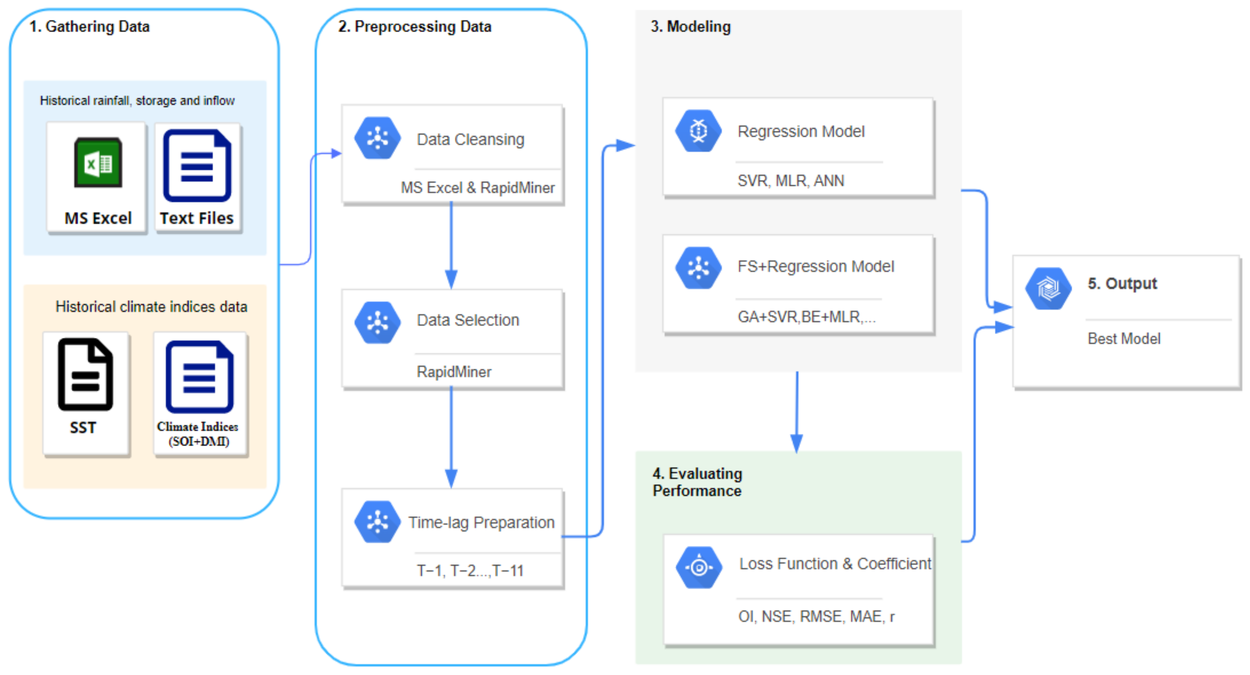
2.1. Research Framework
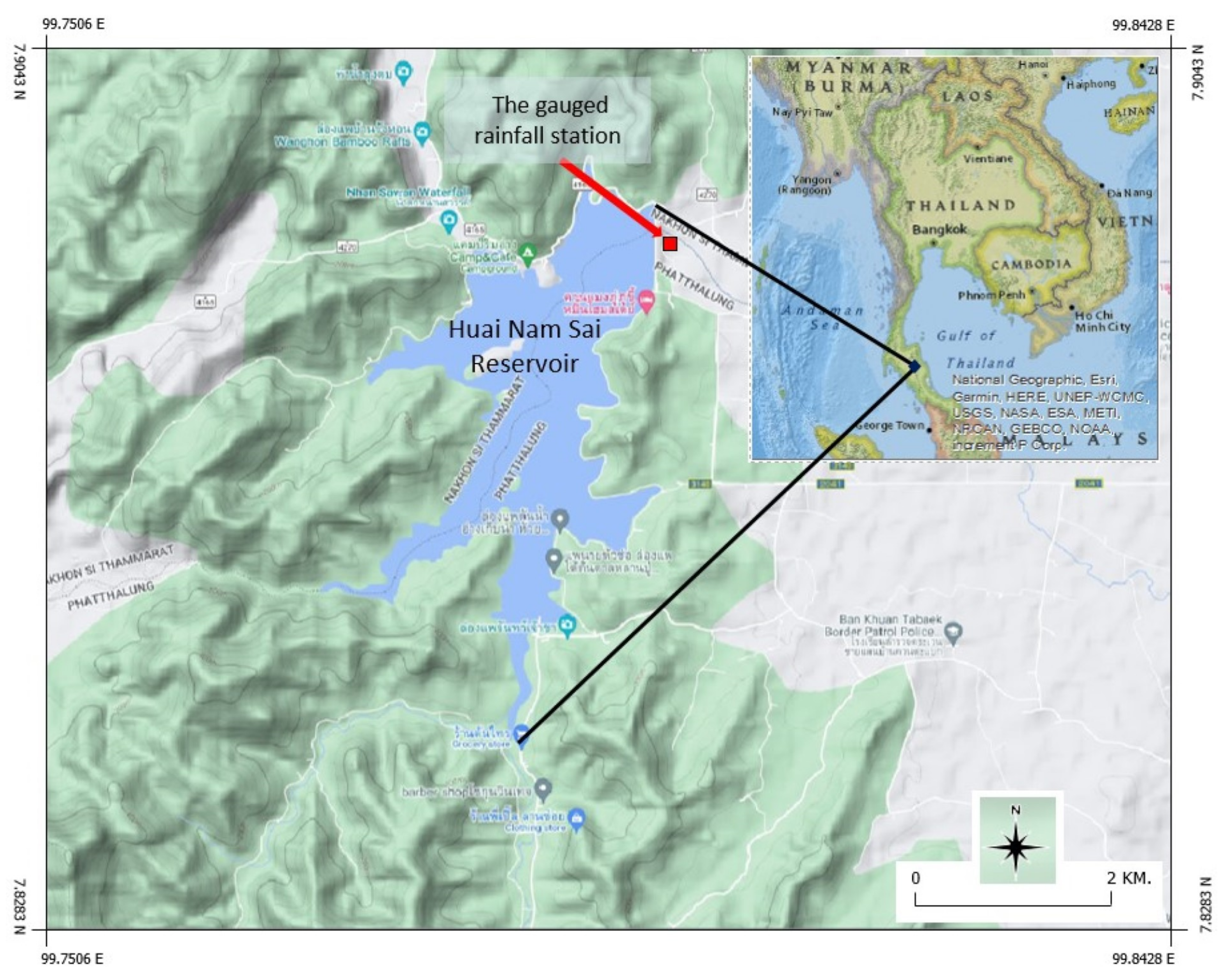
Figure 1 shows the framework with five main steps as follows: (1) gathering data; (2) preprocessing data (i.e., data cleansing, data selection, and lag selection); (3) modeling; (4) evaluating performance; (5) output. The first stage was to collect thirteen variables, including reservoir inflow, reservoir storage, and rainfall, eight SST parameters, and two climate indicators (SOI and DMI). The second stage is divided into two substages: the 12-month lag for preparing historical data and two main strategies for a single output. When the underlying model is nonlinear, the recursive forecasting technique is biased. It is sensitive to estimation errors because, as forecasts go further into the future, estimated values are used more often than actual values [2,36].
The model’s performance in the next level was created by nine machine learning techniques, which are: (1) SVR with linear kernel; (2) SVR with GA (feature selection techniques); (3) SVR with BE (feature selection technique); (4) ANN; (5) ANN with GA; (6) ANN with BE; (7) MLR; (8) MLR with GA; (9) MLR with BE. In 10-fold cross-validation, OI, NSE, RMSE, MAE, and coefficient of correlation (r) are used in the fourth stage to evaluate the model’s performance. Finally, the best model and the set of essential features are shown in Figure 1.

2.2. Study Area

Huai Nam Sai (see Figure 2), a medium-sized reservoir with a capacity of 80 MCM, is one of three main reservoirs in Nakhon Si Thammarat, in Thailand’s southern part, which is a vulnerable area facing severe climate change [37,38]. The Asian Development Bank in 2021 [39] reported that Nakhon Si Thammarat had a warming increase of 1.4 °C between 1851 and 2017. This area is governed by northeast and southwest monsoon winds under a tropical climate. It is therefore appropriate to adopt this study area as representing other reservoirs located in a tropical climate. Huai Nam Sai reservoir is located in Cha-uat District at a latitude of 7°53′33.49″ N and a longitude of 99° 48′32.43″ E. It is an embankment dam with a capacity of 8.00 m in width, 946 m in length, and 40 m in height and was constructed in 1992 by the Royal Irrigation Department (RID). Nowadays, Huai Nam Sai reservoir is operated by the upper Pak Phanang Irrigation and Maintenance Project, Irrigation Office 15, the Royal Irrigation Department, and the Ministry of Agriculture and Cooperatives. It is considered to be the main water supply for the Pak Phanang River Basin. More than 33,913.83 acres of land are irrigated, including the Khlong Mai Siap Weir irrigation system, the Royal Initiative Project’s water supply system, and the Khuan Khanun settlement’s water supply system. Because of this, a total of 20,948.62 acres are directly benefited by the reservoir. The reservoir has several advantages in terms of agriculture and the ecosystem. Crop productivity, off-season kitchen plant production, and rice production all benefit from the reservoir. The Pak Phanang lowland area also acts as a fish breeding habitat and helps prevent flooding.

2.3. Data Used

The monthly data of 216 data sets used in this study (i.e., hydrological data, ocean indices, and sea surface temperature) were gathered between 1998 and 2015 from the following three sources: (1) the Upper Pak Phanang Operation and Maintenance Project, Irrigation Office 15, Royal Irrigation Department (RID), Thailand; (2) the Japan Agency for Marine-Earth Science and Technology (JAMSTEC); and (3) the US National Oceanic and Atmospheric Administration (NOAA) as presented in Table 2.
A monthly reservoir hydrological data set includes rainfall (R), reservoir storage (S), and reservoir inflow (Inf). NOAA and JAMSTEC provide ocean indices and sea surface temperature (SST) data. It was determined that SST could be approximated by the eight input variables, i.e., NINO1+2, ANOM1+2, NINO3, ANOM3, NINO4, ANOM4, NO3.4, and ANOM3.4. The dipole mode index (DMI) and the southern oscillation index (SOI) are two ocean indexes. The Pacific Ocean’s El Niño and La Nina seasons are linked to these two ocean indices. The 12 lag-month (T−1 to T−12) time series of these data, with a total of 156 features, were arranged as input data to forecast the future reservoir inflow data of 3, 6, 9, and 12 months ahead. The fundamental statistical analysis (i.e., maximum (max), minimum (min), average, standard deviation (SD), kurtosis, and skewness of the data used in this study is portrayed in Table 3.

2.4. Machine Learning Techniques

Methods of machine learning were used in the experiments that were conducted for this study. The following is an explanation of how they are described.

2.4.1. Multivariable Linear Regression (MLR)

Regression is a “new” approach that goes back to the eighteenth century (the 1830s to early 1900s) and was established by Sir Francis Galton. He discovered that tall parents tended to have children who were somewhat shorter than themselves, whereas short parents tended to have slightly more elevated children. As a result, the foundations for linear regression (LR) were laid. The key idea of LR is to create a function that analyses and forecasts the value of a target variable when the factors are given their importance. The most common ones are linear regression for numeric prediction. However, there is only one factor that could be supported. Multivariable linear regression (MLR) is a more complex version of linear regression [40]. MLR is one error-based prediction model [41] that produces predictions based on a linear combination of descriptive feature values. In terms of a gradient descent technique through a weight space, this technique applies a preference bias over the order of the linear models it analyses. The MLR model is defined as Equation (1).
Mw d =   w 0 +   w 1 ×   d 1 + +   w m ×   d m =   w 0 + j = 1 m w j × d j
A vector of m defining features is represented by the variable d [m], and the weights [m] are (m + 1). We can make Equation (2) look a little more appealing by establishing a dummy defining feature, d [0], which is almost always equal to 1.
Mw d =   w 0   ×   d 0   +   w 1   ×   d 1 + +   w m   ×   d m =   j = 0 m w j × d j
However, the random starting position is not suitable for predictive analytics problems. The gradient descent is a method that employs a guided search from a random starting point. Using these concepts, the randomly selected weights are softly adjusted in the path of the error surface gradient to move to a new destination on the error surface [28]. When these kinds of methods are used, the optimization works pretty well even when there are a lot of predictors [40].

2.4.2. Support Vector Regression (SVR)

Vapnik’s statistical concept (support vector machine: SVM) is the basis for support vector regression, an artificial intelligence application [30]. With SVR, you can solve complex regression equations [42,43]. Equation (3), function f( x i ) describes the nonlinear relationship between feature x i and objective value y i . In this case, the SVR equation can be described as follows:
f x i = w φ x i + b
In the classification case, w represents the coefficient vector, φ( x i ) represents the differentiation function, and b represents the bias and weight. The C parameter is used to evaluate the significance between losses and complexity. Both the w and b parameters can be indicated from Equation (4).
f R w = 1 2 w 2 + C i = 0 n L y i f x i
When the data are nonlinear, determining the proper dividing line is a major issue. It is impossible to determine the correct dividing line between the data using the soft-margin technique. Kernel functions have been used in numerous studies [31,32] to provide a general solution to this problem. Equation (5) shows the regression function, where k( x i ,x) is the kernel function.
f x = i = 1 l φ i φ i k x i , x + b
In this study, a solution to the problem of function estimation using a least-squares support vector is presented [44], which is expected to be tested with linear kernels as explained in the following Equation (6):
Linear   kernel   k x , x i = x T , x i

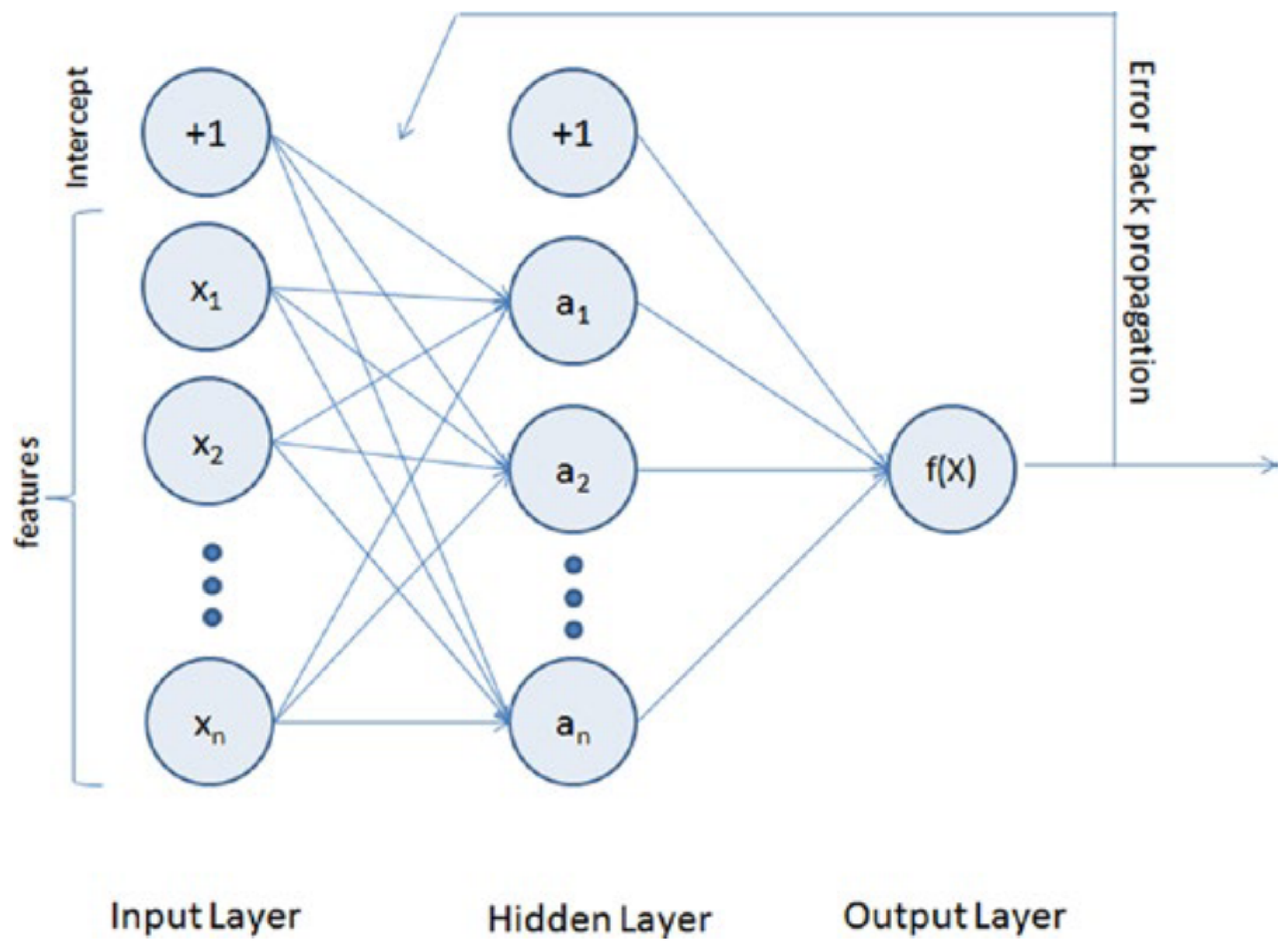
2.4.3. Artificial Neural Networks (ANN)

The functions of artificial neural networks are like those of the human brain. Neurons are the cells that form the human nervous system. They learn from error values that are modified by many neural services. The neural network operates like a black box based on nonlinear high-dimensional data. This model is ideal for prediction work applied in various hydrology and water fields, such as forecasting the volume of water in the dam, precipitation forecasting, reservoir inflow, etc. An ANN is made up of three layers: the original forecasters are in the input layer; created features are in the hidden layer; and the results are in the output layer.
Then, afterward, the aggregated value is converted into a class label using the sign function. The sign function performs the function of activation as in Equation (5). Different activation functions can be used to mimic various machine learning models, such as least-squares with numerical parameters, support vector machines, and logistic regression models. As shown in Figure 3, a bias neuron can be used to implement the bias as the weight of input. This is accomplished by inserting a neuron into the output node that always transfers a value of 1 [45]. Forecasting future inflows or any hydrological variable is made possible by the ability of the ANN forecasting model to do so purely on historical data. Forecasting inflows with other types of forecasting models typically necessitate the inclusion of additional variables. Accurately predicting how much water will flow into a reservoir in the future can help this facility run smoothly.

2.4.4. Genetics Algorithm (GA)

The genetic algorithm technique (GA) was initially presented by John Holland [47]. Similar to Darwin’s notion of natural selection and genetic evolution, it is a famous metaheuristic search approach [22]. As a result of randomization, the fitness function analyses the quality of a result obtained in the evolutionary stage. The GA has three important operators: at least one-point crossover or homolog crossover is used to swap genes between two chromosomes, with the mutation operator associated with gene pairing and selection determining the presence of the fittest. SVR can integrate GA for parameter optimization and feature subset selection. There are four steps GA has to follow: (1) randomly create a preliminary population; (2) approximate the fitness value between chromosomes in the population; (3) implement genetic operations (crossover, mutation, and selection); (4) if the conditions are correct, terminate the algorithm; return to step 2 [32].

2.4.5. Backward Eliminations (BE)

Two common search strategies are the forward and backward approaches for selecting variable subsets. The forward method adds one variable and validates the appropriate model for each step with a practical criterion. The forward technique is terminated when there is no better feature subset than the present subset [41]. This method is a widespread implementation of the greedy local feature search strategy. When the number of variables of applicants (N) is minimal, a prediction model may be chosen by calculating an adequate criterion for all potential sub-sets (such as RMSE and the cross-validation error) [48].
Many studies included these approaches with other methods. For example, Valente and Maldonado presented a time series analysis and proposed an advanced SVR technique. An efficient forward feature selection technique has been submitted for analyzing multi-seasonal high-frequency time series [49]. There are disadvantages to using forward selection as well. When using forward selection, the addition of a new variable to the model has the potential to render one of the previously included variables insignificant; nevertheless, the previously included variable cannot be removed from the model [50].
The backward elimination method (BE) is a prominent choice for sequential forward selection. BE starts with a wide-ranging set of input variables and then eliminates variables from that set repeatedly until a certain terminating condition is correct. The performance of BE can be evaluated by the Perf function, which measures a set of input variables and returns their performance correlation to a certain statistical model [6], as shown in Algorithm 1 [51]. Even though it requires a great deal of computer time, the iterative BE approach is an effective technique for evaluating a model.
Algorithm 1 Backward Elimination (BE) for Reservoir Inflow Forecasting
Input: Data set D, Target T. Output: Selected Variables SV
//D: Huai Nam Sai Reservoir, T: Inflow, SV: R, S, Inf., Climate Indices (10 parameters)
iterate until SV does not change
1: while SV changes do
2://Identify the worst variable Vworst out of all selected variables SV, according to Perf
3:   Vworst ← argmax (V∈SV) Perf(S\V)
4://Remove Vworst if it does not decrease performance according to criterion C
5:   if Perf(SV\Vworst) ≥ Perf(SV) then
6:     SV ← SV\Vworst
7: end if
8: end while
9: return SV
This study chose the most suitable attributes using GA and BE for the MLR, SVR, and ANN techniques. In SVR modeling, the values assigned to parameters σ, C, and ε are 0.001, 0.001, and 0.001, respectively. The linear type of kernel is selected and used both during the training and test steps. The settings for the training cycle, learning rate, and momentum were each set to 0.9 for the ANN technique. The training cycle was set to 200, and the learning rate was set to 0.01.

2.5. Experimental Setup

The nine experiments described in Table 4 were designed for our study. Three techniques of machine learning, namely ANN, SVR (Linear kernel), and MLR, were utilized. As stated in Section 2.4.4 and Section 2.4.5, the influence of GA and BE feature selection techniques were investigated. This case study used a 64-bit computing environment with 8 GB of RAM to run several numerical experiments. RapidMiner Studio 8.1 was utilized to carry out this investigation.

2.6. Statistical Performance Measures

This study used 10-fold cross-validation and deployed five acceptable statistical performance measures, i.e., overall index (OI), Nash–Sutcliffe efficiency (NSE), mean absolute error (MAE), root mean square error (RMSE), and correlation coefficient (r). Numerous studies demonstrate the suitability of these statistical performance measures for evaluating the precision of hydrological models [9,13,19,23,52,53,54,55]. The following equations define OI, NSE, RMSE, MAE, and r.
The OI indicator is a criterion that indicates the overall performance of a model, with values ranging between −∞ and 1 [56]. The model’s performance is favorable if the higher OI is closer to 1.
O I = 1 2 2 i = 1 n Q o Q p 2 n Q o , m a x Q b , m i n i = 1 n Q o Q p 2 i = 1 n Q o Q ¯ o 2
NSE is utilized to evaluate the prediction performance of hydrological models. The range of NSE values is between −∞ and 1, where NSE = 1.0 is optimal.
N S E = 1 i = 1 n Q p Q o 2 i = 1 n Q o Q ¯ o 2
The value of RMSE shows the degree of the error. RMSE evaluates the average amount of error between the predicted and observed values. MAE shows the average absolute deviation of the estimates from the actual value. The model is very effective when the RMSE and MAE values approach 0.
R M S E = i = 1 n Q o Q p 2 n
M A E = i = 1 n Q o Q p n
Widely used to determine the linear relationship between observed and predicted data, the correlation coefficient (r) is a measure of linear correlation. The range from −1 to 1 for the value of r indicates a perfect negative or positive correlation, respectively.
r = i = 1 n Q o Q ¯ o Q p Q ¯ p i = 1 n Q o Q ¯ o 2 · i = 1 n Q p Q ¯ p 2
where Q o denotes the observed reservoir inflow, Q p denotes the predicted reservoir inflow, Q ¯ o denotes the average observed reservoir inflow, Q ¯ p denotes the average predicted reservoir inflow, Q o , m a x denotes the maximum observed reservoir inflow, Q o , m i n denotes the minimum observed reservoir inflow, and n denotes the number of reservoir inflow data.

3. Results and Discussion

This section presents the performance comparison of three essential ML methods with climate indices parameters to find the best ML technique with or without a feature selection method for reservoir inflow forecasting. The forecasting model was then tested using the remaining years of data after the model parameters were derived using the training data set (17 years). They measure the accuracy of popular models in forecasting the amount of water flowing into a reservoir or dam from the monthly time-series data set (216 records). This error is accomplished by calculating the minimum error value. RMSE, MAE, and NSE were utilized in this investigation to measure errors. Local hydrology and global climate change are intertwined, with the former constantly impacting the latter. As a result, lagging information is introduced into model inputs, causing correlation effects in variables such as inflow, precipitation, and climate phenomenon indices.

3.1. Results of Feature Selection

Table 5 provides a summary of the total number of parameters for each ML method in four lead times (T + 3, T + 6, T + 9, and T + 12). At three-month lead times (T + 3), GA is the model with the fewest number of features, where GA-ANN uses 70 parameters for related variables, followed by GA-SVR and BE-ANN with 82 and 152 features, respectively. During this time, it appears that the parameters that BE-ANN can eliminates are ANOM1+2 (t−7), Inf (t−1), and NO3.4. The GA was able to reduce the number of input parameters by 47–53%. GA-ANN has the highest efficiency in terms of parameter reduction, with 85 parameters. Similar patterns of performance were seen in the second period (T + 6) compared to the first. The lowest number of parameters (67) was used by GA-ANN, with GA-SVR coming in second (90 parameters). Third, four models reduced the number of parameters by the same amount: BE-ANN, GA-MLR, BE-MLR, and BE-SVR. BE-ANN eliminate only the parameters Inf (t−1). However, none of the four methods reduced the number of parameters by more than one. In the six-month lead time (T + 9), GA-ANN was the model that used the fewest parameters across all periods (59) or reduced the number of parameters by more than 60%, followed by GA-SVR and BE-ANN, which used 72 and 151 parameters, respectively. The parameters that BE-ANN can remove are Inf (t−1), ANOM1+2 (t−8), SOI (t−6), and ANOM3 (t−7). The results at the final lead time (T + 12) were similar to the first three lead times. The GA-ANN model reduced the number of input parameters by 84, followed by the reduced number used by the GA-SVR model, which used 76 input parameters. This results in similarity to the T + 6 lead time. There are four other models: BE-ANN, GA-MLR, BE-MLR, and BE-SVR. These models only need one input parameter. At this time, BE-ANN can reduce only the parameters Inf (t−1). Therefore, the NINO1+2 index and the 12-month lagging water storage were selected as input variables for the reservoir. This is consistent with what was discovered in [9]. The developed model’s efficacy results revealed that GA-induced improvements in quantifying parameters associated with ANN and SVR were more significant than 60% and 45%, respectively. The experimental results agreed with experiments [22,36].

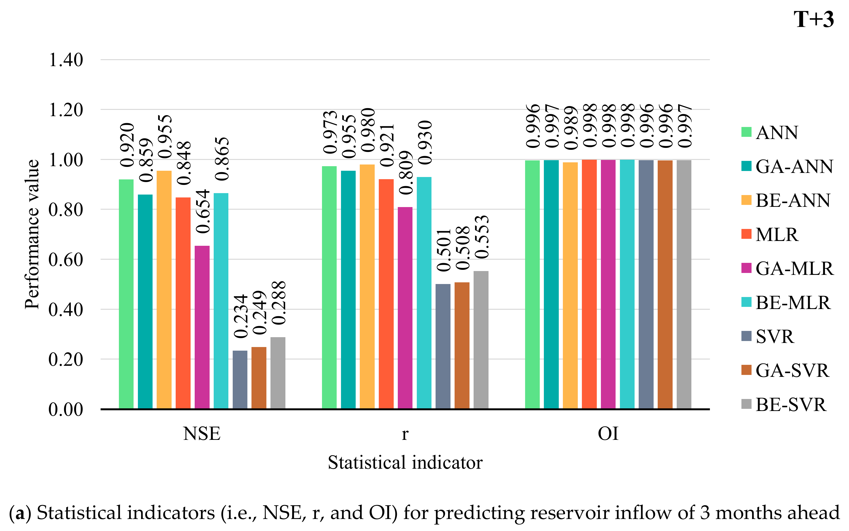
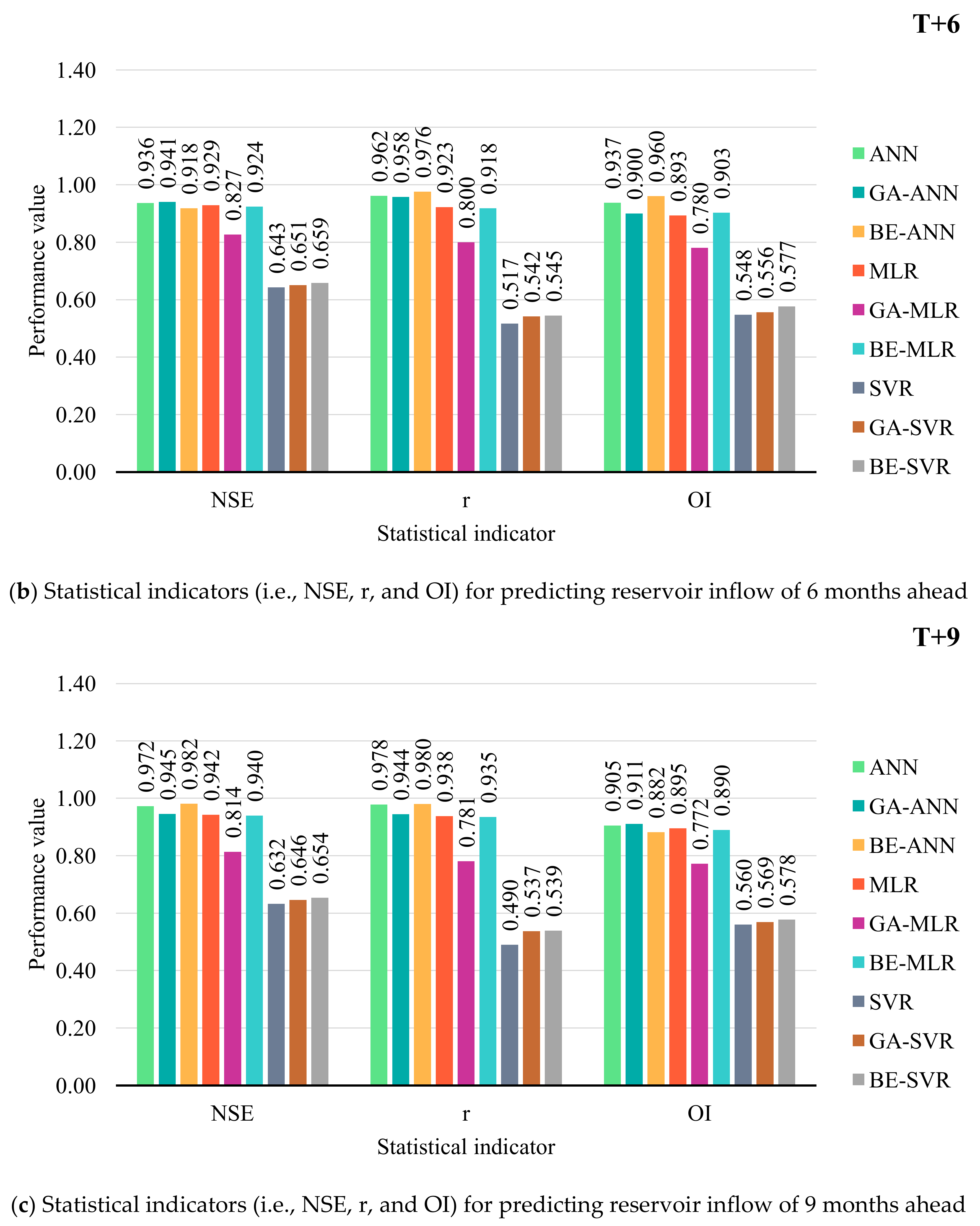
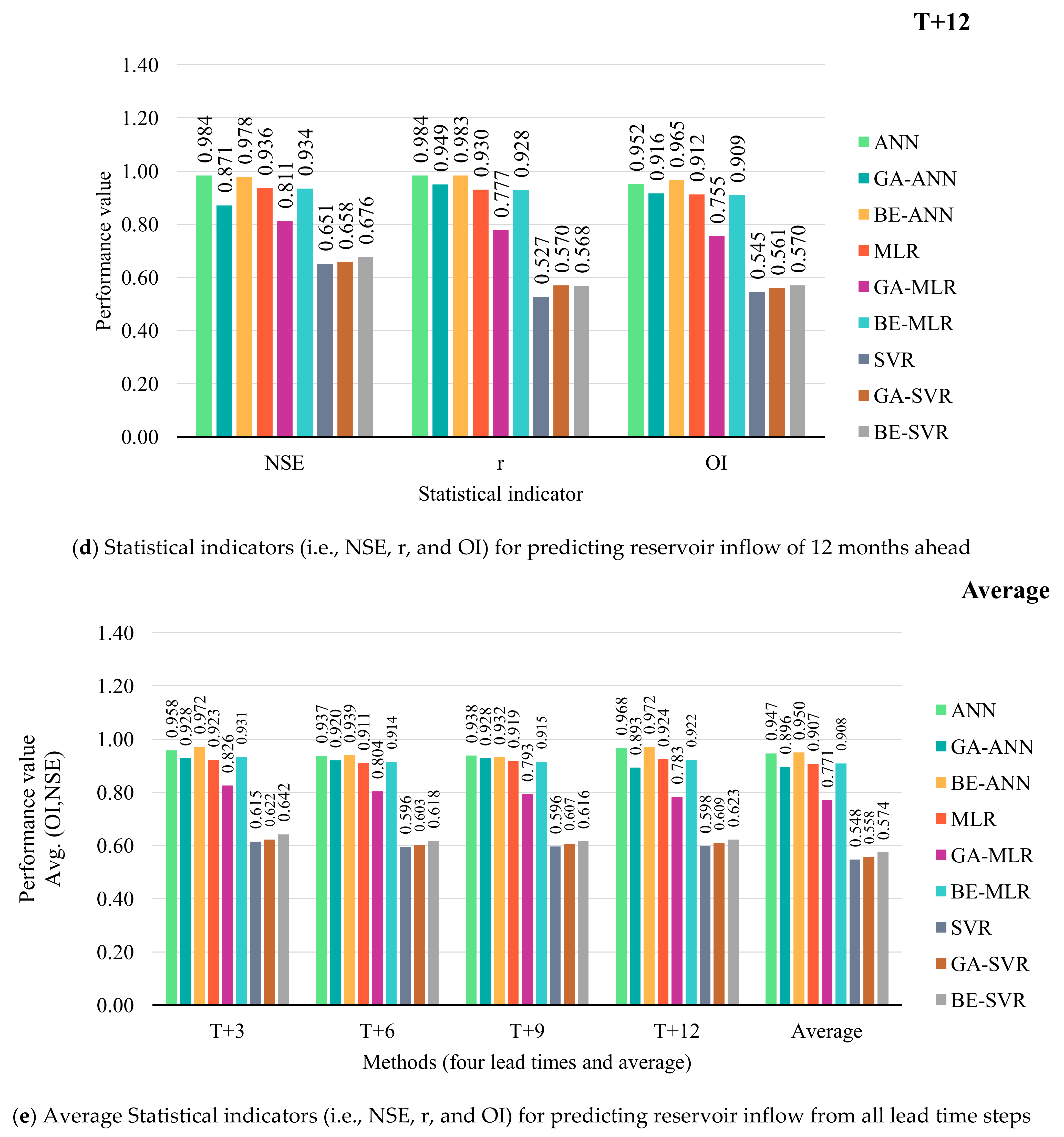
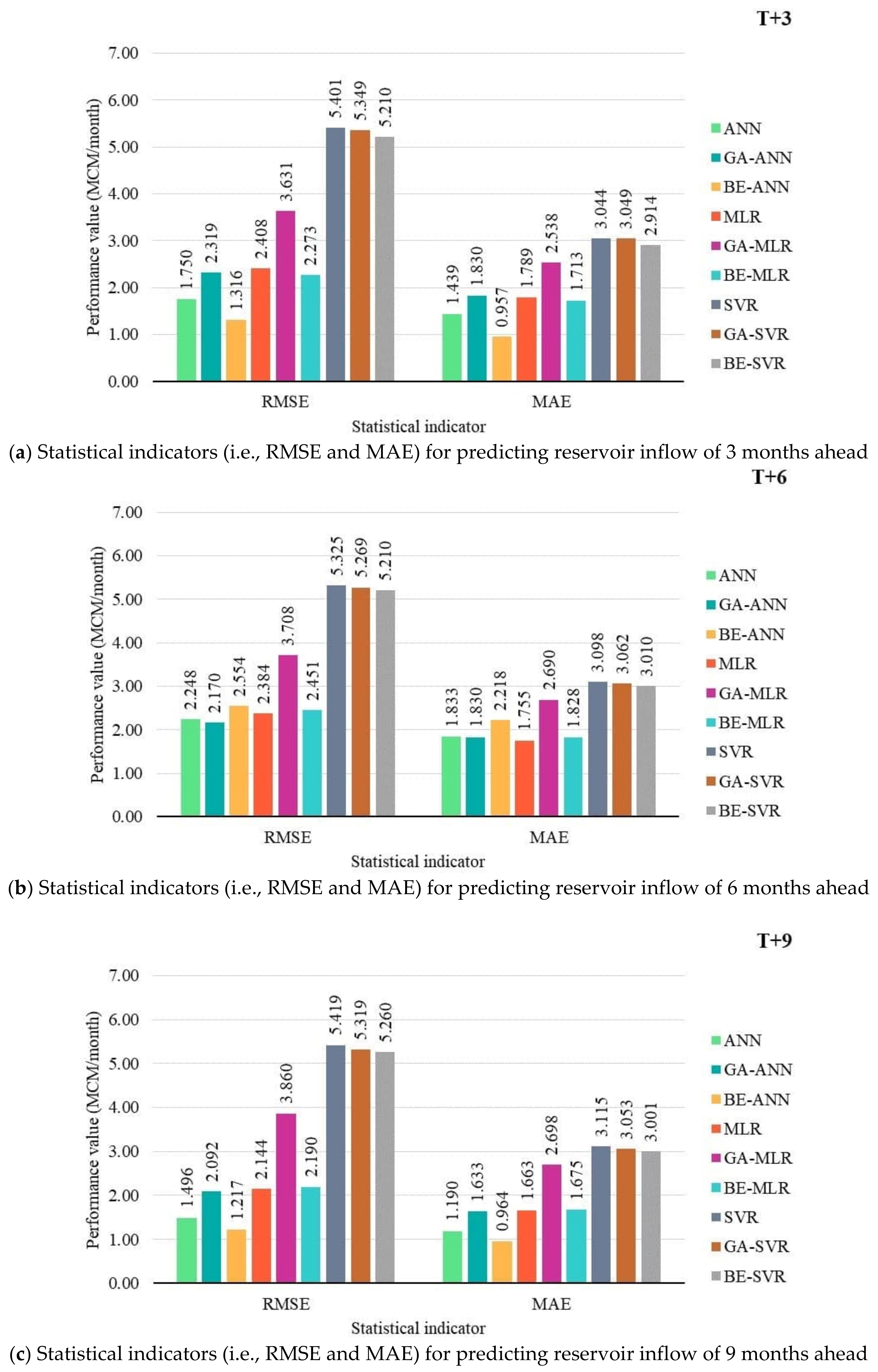
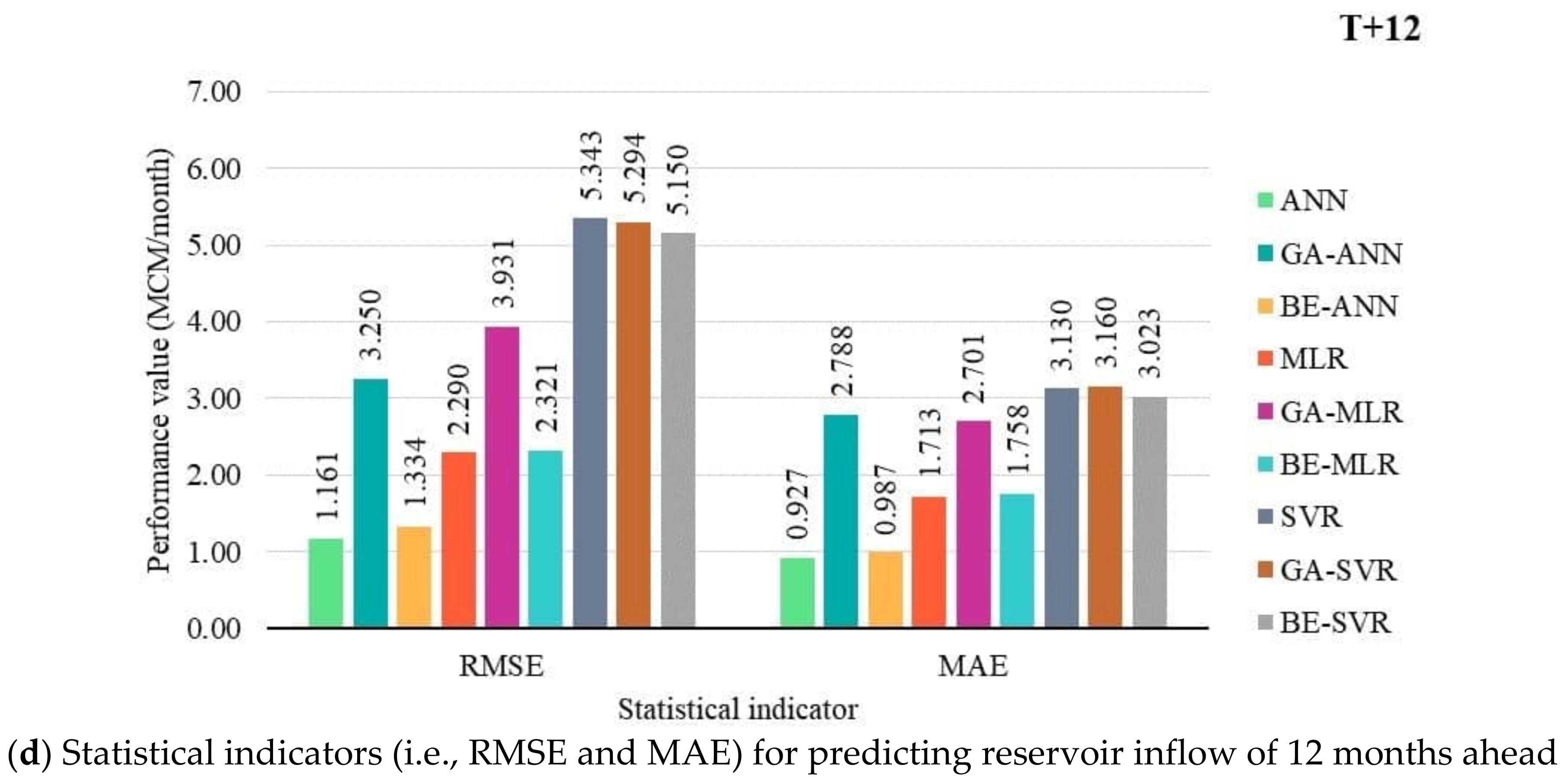
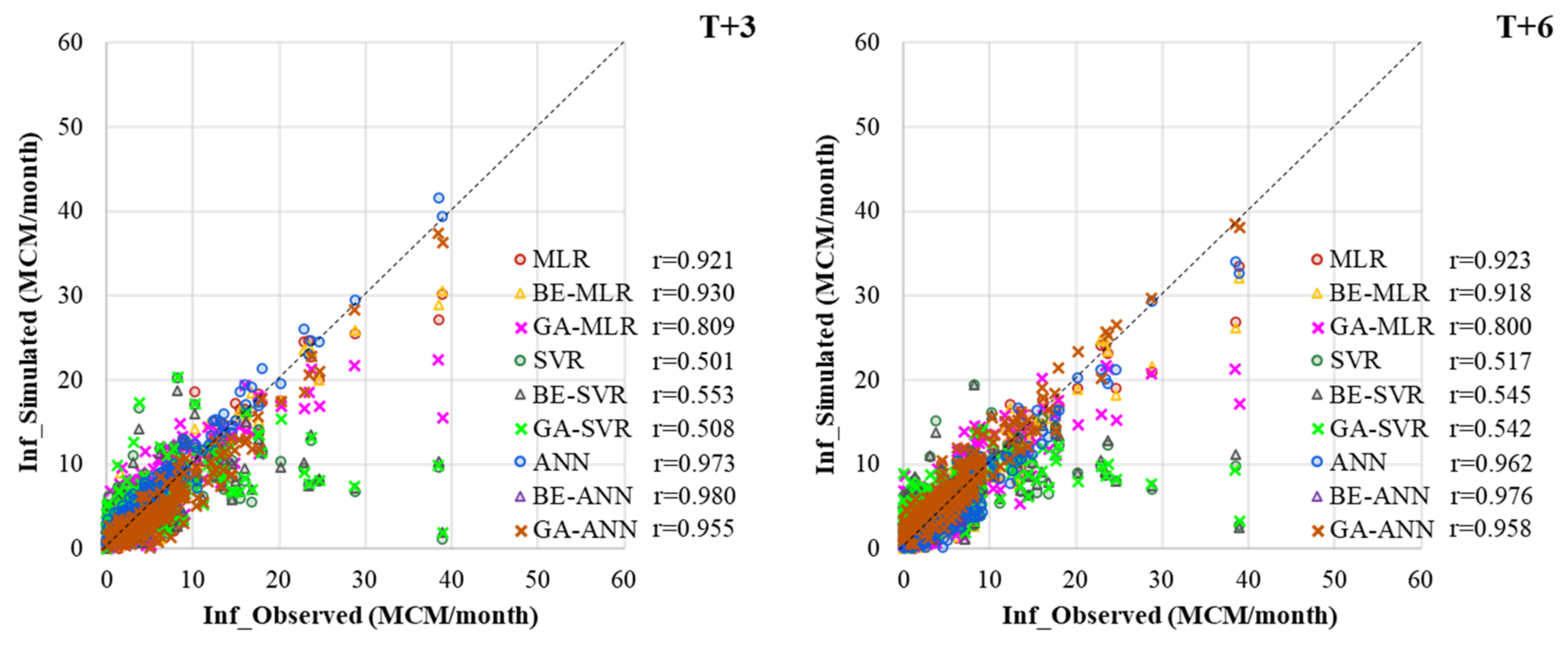
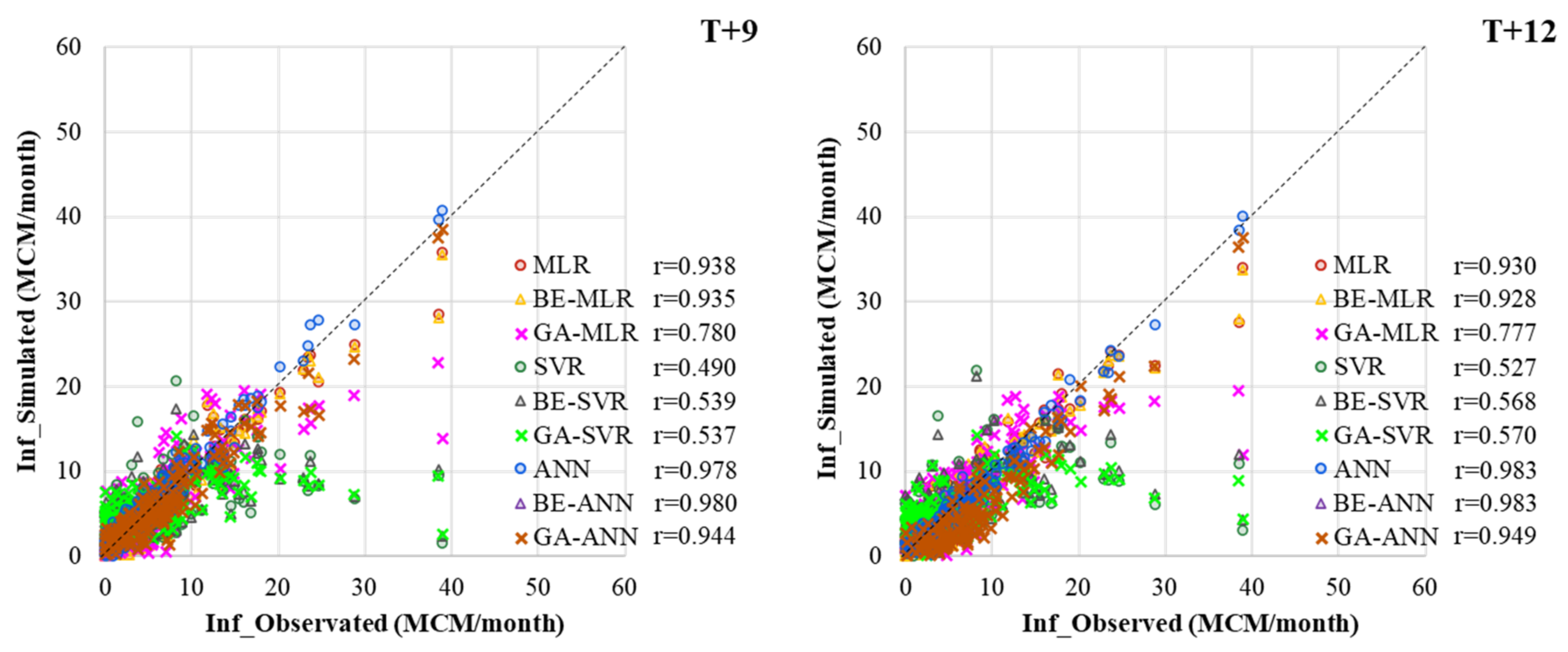
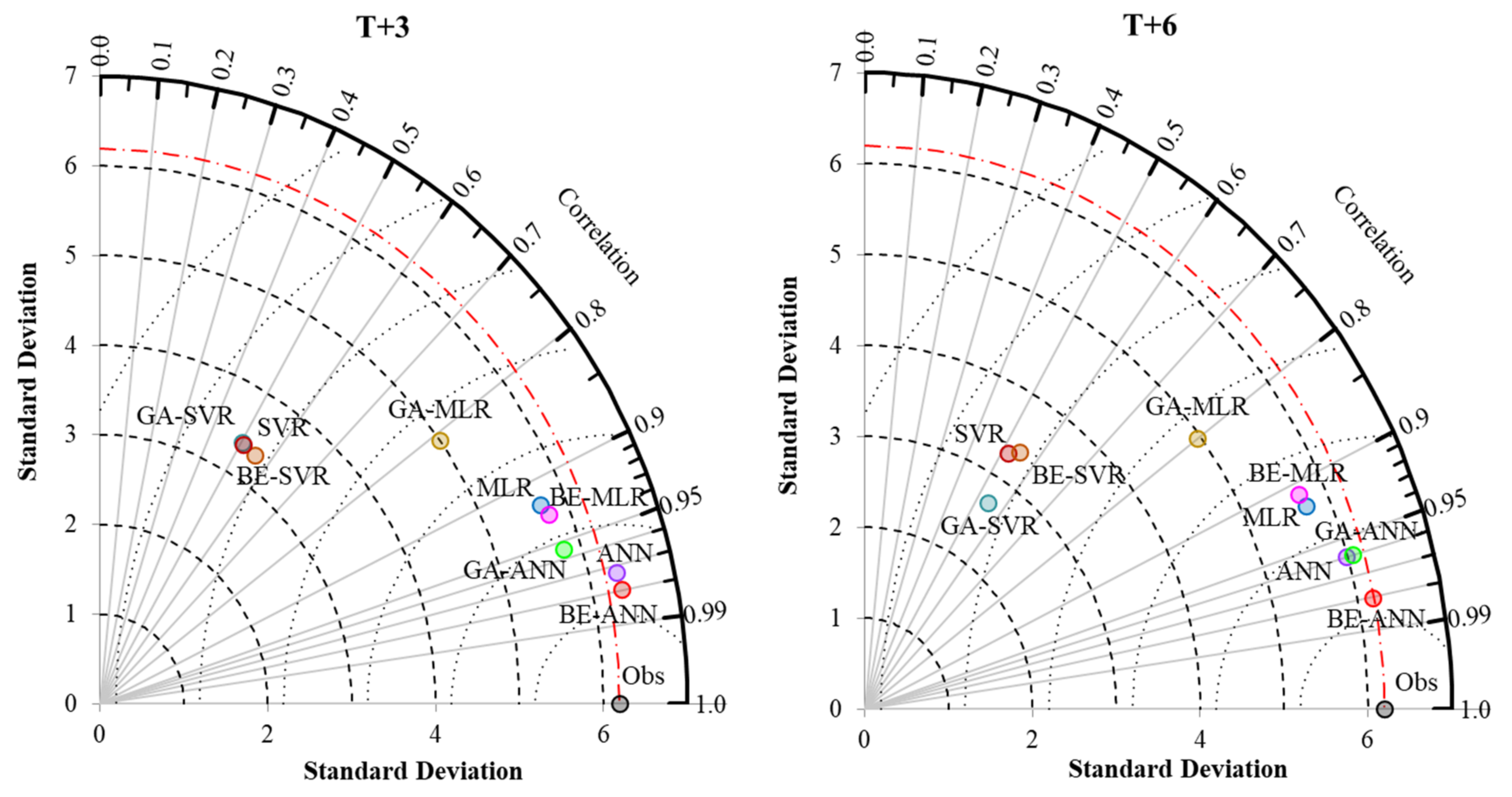
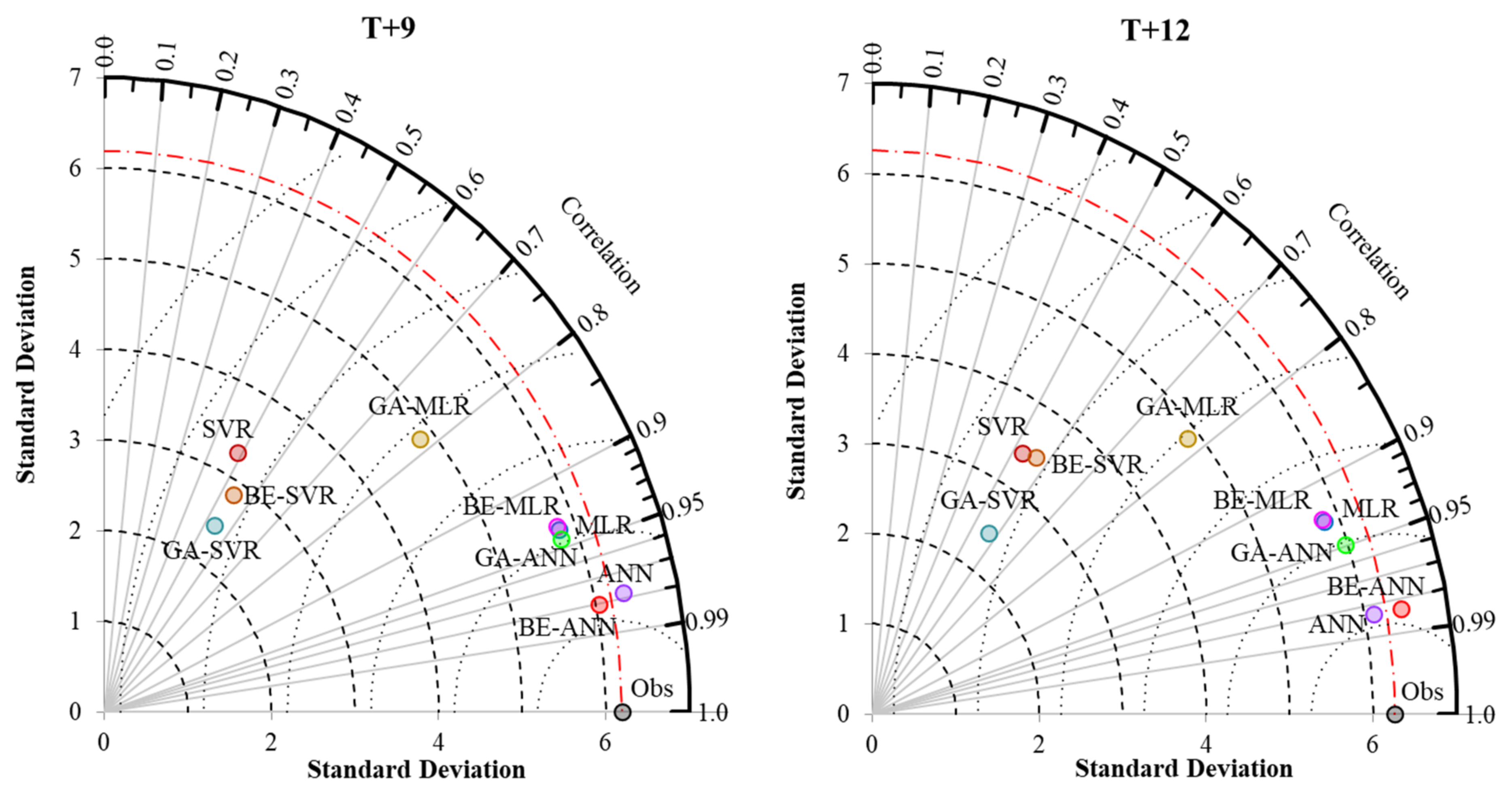
3.2. Performance Comparison of Prediction Models

MLR, ANN, SVR, and Hybrid with BE and GA

Figure 4a–d show the comparison of prediction accuracy results (i.e., OI, NSE, and r) of nine machine learning models with a lead time of 3, 6, 9, and 12 months. Figure 4e also provides the average value of OI and NSE for each lead time step and its average for all lead time steps. Figure 5 presents the comparison of nine ML models’ prediction errors (i.e., RMSE and MAE) for four lead times.
At the lead time of three months (T + 3), the BE-ANN model showed high prediction accuracy, with average an OI and NSE of 0.972, an OI of 0.989, NSE of 0.955, r of 0.980, RMSE of 1.136 MCM/month, and MAE of 0.957 MCM/month. In contrast, ANN and BE-MLR offer less performance than BE-ANN with average an OI and NSE of 0.958 and 0.931, an OI of 0.996 and 0.998, NSE of 0.920 and 0.865, r of 0.973 and 0.930, RMSE of 1.750 and 2.273 MCM/month, and MAE of 1.439 and 1.713 MCM/month, respectively. That means that BE-ANN is the best machine learning model at this lead time. On the other hand, the top three least effective prediction techniques are SVR, GA-SVR, and BE-SVR, with an average OI and NSE of 0.615, 0.622, and 0.642, an OI of 0.996, 0.996, and 0.997, r of 0.501, 0.508, and 0.553, RMSE of 5.401, 5.349, and 5.210 MCM/month, and MAE of 3.044, 3.049, and 2.914 MCM/month, respectively.
At the lead time of six months (T + 6), similar to the previous lead time, the BE-ANN model showed the highest prediction accuracy, with an average OI and NSE of 0.939, an OI of 0.960, NSE of 0.918, r of 0.976, RMSE of 1.316 MCM/month, and MAE of 0.957, 1.316 MCM/month. Therefore, BE-ANN is the best ML technique at this point. However, SVR, GA-SVR, and BE-SVR are the top three least effective prediction methods, with an average OI and NSE of 0.596, 0.603, and 0.618, an OI of 0.548, 0.556, and 0.577, and r of 0.517, 0.542, and 0.545, RMSE of 5.325, 5.269, and 5.210 MCM/month, and MAE of 3.098, 3.062, and 3.010 MCM/month, respectively.
It should be noted that at a lead time of nine months (T + 9), the ANN model showed the highest prediction accuracy, with an average OI and NSE of 0.938, an OI of 0.905, NSE of 0.972, r of 0.978, RMSE of 1.496 MCM/month, and MAE of 1.190 MCM/month, respectively. BE-ANN and GA-ANN models performed second and third best during this period, with an average OI and NSE of 0.932 and 0.928, an OI of 0.882 and 0.911, NSE of 0.982 and 0.945, r of 0.980 and 0.944, RMSE of 1.207 and 2.092 MCM/month, and MAE of 0.964 and 1.633 MCM/month, respectively.
At the lead time of twelve months (T + 12), the BE-ANN model showed the highest prediction accuracy, with an average OI and NSE of 0.972, an OI of 0.965, NSE of 0.978, r of 0.983, RMSE of 1.334 MCM/month, and MAE of 0.987 MCM/month. While ANN and MLR offer worse performance than BE-ANN with an average OI and NSE of 0.968 and 0.924, an OI of 0.952 and 0.912, NSE of 0.984 and 0.936, r of 0.984 and 0.930, RMSE of 1.162 and 2.290 MCM/month, and MAE of 0.927 and 1.713 MCM/month, respectively.
Regarding the nine ML techniques above, BE-ANN provided the best on-average performance for all of the lead times (see Figure 4e). Therefore, it is the most suitable method for predicting monthly time-series data in advance. In addition, it provided the highest value of an average OI and NSE of 0.95, an average OI, NSE, and r of 0.9418, 0.9581, and 0.9798, respectively. It should be noted that both FS techniques (i.e., GA and BE) could improve the forecasting performance of SVR for all of the lead times, but they could not improve the forecasting performance of MLR for all of the lead times. In comparison, only BE can improve the forecasting performance of ANN for all of the lead times except twelve-time-ahead. The suitable, developed model could reduce the error by more than 5000 m3/month. Neither the BE nor the GA was suitable for MLR, SVR, and ANN for twelve-time-ahead. ANN is more suitable for planning annual water management actions than quarterly water management actions. Unlike GA-ANN, which is considered suitable for 6-month water management action planning, BE-ANN is best suited for quarterly and 9-month water management action planning. The Huai Nam Sai Reservoir’s operational plans could benefit from this technique.
Figure 6 presents the scatter plot of the observed and simulated reservoir inflow of nine machine learning techniques for four lead times. The graph shows the relationship between the observed and the simulated inflow obtained from ANN, BE-ANN, GA-ANN, MLR, BE-MLR, GA-MLR, SVR, BE-SVR, and GA-SVR for four lead times. The perfect line is depicted as the 45-degree diagonal solid line. Overall, it could be observed that at approximately below 20 MCM/month, all developed models gave a rather good prediction accuracy due to them giving a value close to the perfect line. However, high reservoir inflow prediction gave an underestimation for all of the considered lead times. This is generally found in reservoir inflow forecasting [2,20,57].
Figure 7 represents a Taylor diagram that compares nine ML models for forecasting the monthly reservoir inflow of Huai Nam Sai Reservoir. The BE-ANN model provided the highest value of r for lead times 3, 6, and 9 months, while ANN gave the highest value of r for a lead time of 12 months. In addition, BE-ANN and ANN models gave a standard deviation value very close to the observed reservoir inflow time series for all lead times. For a lead time of 6 months, GA-ANN also provided a standard deviation value very close to the observed reservoir inflow time series.

4. Conclusions

This study proposed and examined the performance of hybrid models by combining ML techniques (i.e., MLR, SVR (linear kernel), and ANN) with FS techniques (i.e., GA and BE) for predicting the monthly reservoir inflow. In addition to hydrological data (monthly rainfall and reservoir inflow data), climate indices were used as the input data. The proposed model was investigated based on the Huai Nam Sai Reservoir, Nakhon Si Thammarat, Thailand, which is governed by a tropical climate. This study area has been facing climate change effects. The key findings of this study can be summarized as follows:
  • Feature selection methods (i.e., GA and BE) could improve the performance of SVR and ANN for predicting monthly reservoir inflow forecasting, but they have no effects on MLR. GA and BE could select better features for SVR for all of the lead times. Only BE could make compelling selection features for ANN by improving its performance for almost all of the lead times (i.e., T + 3, T + 6, T + 9) except for twelve lead times (T + 12). GA could overwhelmingly reduce the number of features by more than 60% and 45% for ANN and SVR, respectively. Although BE could improve the ANN and SVR’s performance by approximately 1% over GA, it required a much higher number of features.
  • With average an OI and NSE, BE-ANN provides the best performance for 3, 6, and 12 months ahead (T + 3, T + 6, and T + 12). While ANN was suitable for 9 months ahead only. SVR, GA-SVR, and BE-SVR, however, are the least effective of the top three prediction methods.
  • Different developed forecasting models were suitable for different reservoir inflow forecasting time-step-ahead. That is, BE-ANN gave the best performance for 3 and 9 months ahead (T + 3 and T + 9), whilst GA-ANN was suitable for semi-annually reservoir inflow forecasting. Finally, ANN provided the best model for annual reservoir inflow forecasting. From the overall results, all SVR-based models (i.e., SVR, GA-SVR, and BE-SVR) gave the lowest performance by giving the lowest values of OI, NSE, and r and the highest values of RMSE and MAE.
  • To increase the forecasting models’ performance on reservoir inflow, future studies would have to focus on the extreme events that are frequently happening presently due to climate change effects, i.e., very high peak reservoir inflow, crucially leading to helping reservoir regulators with optimal reservoir operations.

Author Contributions

Conceptualization, P.D. and N.K.; methodology, J.W., P.D. and N.K.; software, J.W.; validation, P.D. and N.K.; formal analysis, J.W.; investigation, J.W., P.D. and N.K.; resources, J.W. and N.K.; data curation, J.W.; writing—original draft preparation, J.W., P.D. and N.K.; writing—review and editing, P.D., N.K., Q.B.P. and N.T.T.L.; visualization, J.W.; supervision, P.D., N.K. and Q.B.P.; project administration, P.D. and N.K.; funding acquisition, J.W., Q.B.P. and N.T.T.L. All authors have read and agreed to the published version of the manuscript.

Funding

This research was partially funded by the Ministry of Higher Education, Science, Research, and Innovation, Thailand under grant number 6/2565. The authors are gratefully acknowledged.

Institutional Review Board Statement

Not applicable.

Informed Consent Statement

Not applicable.

Data Availability Statement

Not applicable.

Conflicts of Interest

The authors declare no conflict of interest.

References

  1. Chiamsathit, C.; Adeloye, A.J.; Bankaru-Swamy, S. Inflow forecasting using artificial neural networks for reservoir operation. Proc. Int. Assoc. Hydrol. Sci. 2016, 373, 209–214. [Google Scholar] [CrossRef] [Green Version]
  2. Liao, S.; Liu, Z.; Liu, B.; Cheng, C.; Jin, X.; Zhao, Z. Multistep-ahead daily inflow forecasting using the ERA-Interim reanalysis data set based on gradient-boosting regression trees. Hydrol. Earth Syst. Sci. 2020, 24, 2343–2363. [Google Scholar] [CrossRef]
  3. Liu, Y.; Zhang, K.; Li, Z.; Liu, Z.; Wang, J.; Huang, P. A hybrid runoff generation modelling framework based on spatial combination of three runoff generation schemes for semi-humid and semi-arid watersheds. J. Hydrol. 2020, 590, 125440. [Google Scholar] [CrossRef]
  4. Chen, Z.; Liu, Z.; Yin, L.; Zheng, W. Statistical analysis of regional air temperature characteristics before and after dam construction. Urban Clim. 2022, 41, 101085. [Google Scholar] [CrossRef]
  5. Yin, L.; Wang, L.; Keim, B.D.; Konsoer, K.; Zheng, W. Wavelet Analysis of Dam Injection and Discharge in Three Gorges Dam and Reservoir with Precipitation and River Discharge. Water 2022, 14, 567. [Google Scholar] [CrossRef]
  6. Lee, D.; Kim, H.; Jung, I.; Yoon, J. Monthly Reservoir Inflow Forecasting for Dry Period Using Teleconnection Indices: A Statistical Ensemble Approach. Appl. Sci. 2020, 10, 3470. [Google Scholar] [CrossRef]
  7. Allawi, M.F.; Hussain, I.R.; Salman, M.I.; El-Shafie, A. Monthly inflow forecasting utilizing advanced artificial intelligence methods: A case study of Haditha Dam in Iraq. Stoch. Hydrol. Hydraul. 2021, 35, 2391–2410. [Google Scholar] [CrossRef]
  8. Weekaew, J.; Ditthakit, P.; Kittiphattanabawon, N. Reservoir Inflow Time Series Forecasting Using Regression Model with Climate Indices. Recent Adv. Inf. Commun. Technol. 2021, 251, 127–136. [Google Scholar]
  9. Kim, T.; Shin, J.Y.; Kim, H.; Kim, S.; Heo, J.H. The use of large-scale climate indices in monthly reservoir inflow forecasting and its application on time series and artificial intelligence models. Water 2019, 11, 374. [Google Scholar] [CrossRef] [Green Version]
  10. Vadiati, M.; Rajabi Yami, Z.; Eskandari, E.; Nakhaei, M.; Kisi, O. Application of artificial intelligence models for prediction of groundwater level fluctuations: Case study (Tehran-Karaj alluvial aquifer). Environ. Monit. Assess. 2022, 194, 1–21. [Google Scholar] [CrossRef]
  11. Samani, S.; Vadiati, M.; Azizi, F.; Zamani, E.; Kisi, O. Groundwater Level Simulation Using Soft Computing Methods with Emphasis on Major Meteorological Components. Water Resour. Manag. 2022, 36, 3627–3647. [Google Scholar] [CrossRef]
  12. Ditthakit, P.; Pinthong, S.; Salaeh, N.; Binnui, F.; Khwanchum, L.; Pham, Q.B. Using machine learning methods for supporting GR2M model in runoff estimation in an ungauged basin. Sci. Rep. 2021, 11, 19955. [Google Scholar] [CrossRef] [PubMed]
  13. Zhou, Y.; Guo, S.; Chang, F.J. Explore an evolutionary recurrent ANFIS for modelling multi-step-ahead flood forecasts. J. Hydrol. 2019, 570, 343–355. [Google Scholar] [CrossRef]
  14. Kao, I.F.; Liou, J.Y.; Lee, M.H.; Chang, F.J. Fusing stacked autoencoder and long short-term memory for regional multistep-ahead flood inundation forecasts. J. Hydrol. 2021, 598, 126371. [Google Scholar] [CrossRef]
  15. Chang, L.C.; Liou, J.Y.; Chang, F.J. Spatial-temporal flood inundation nowcasts by fusing machine learning methods and principal component analysis. J. Hydrol. 2022, 612, 128086. [Google Scholar] [CrossRef]
  16. Makridakis, S. Time series prediction: Forecasting the future and understanding the past. Int. J. Forecast. 1994, 10, 463–466. [Google Scholar] [CrossRef]
  17. Wang, S.; Zhang, K.; Chao, L.; Li, D.; Tian, X.; Bao, H.; Chen, G.; Xia, Y. Exploring the utility of radar and satellite-sensed precipitation and their dynamic bias correction for integrated prediction of flood and landslide hazards. J. Hydrol. 2021, 603, 126964. [Google Scholar] [CrossRef]
  18. Tongsiri, J.; Kangrang, A. Prediction of Future Inflow under Hydrological Variation Characteristics and Improvement of Nam Oon Reservoir Rule Curve using Genetic Algorithms Technique. Mahasarakham Univ. J. Sci. Technol. 2018, 37, 775–788. [Google Scholar]
  19. Valipour, M.; Banihabib, M.E.; Behbahani, S.M.R. Parameters estimate of autoregressive moving average and autoregressive integrated moving average models and compare their ability for inflow forecasting. J. Math. Stat. 2012, 8, 330–338. [Google Scholar] [CrossRef] [Green Version]
  20. Lin, G.F.; Chen, G.R.; Huang, P.Y. Effective typhoon characteristics and their effects on hourly reservoir inflow forecasting. Adv. Water Resour. 2010, 33, 887–898. [Google Scholar] [CrossRef]
  21. Yang, T.; Asanjan, A.A.; Welles, E.; Gao, X.; Sorooshian, S.; Liu, X. Developing reservoir monthly inflow forecasts using artificial intelligence and climate phenomenon information. Water Resour. Res. 2017, 53, 2786–2812. [Google Scholar] [CrossRef]
  22. Cheng, C.T.; Feng, Z.K.; Niu, W.J.; Liao, S.L. Heuristic methods for reservoir monthly inflow forecasting: A case study of xinfengjiang reservoir in pearl river, China. Water 2015, 7, 4477–4495. [Google Scholar] [CrossRef]
  23. Elbeltagi, A.; Kumar, M.; Kushwaha, N.L.; Pande, C.B.; Ditthakit, P.; Vishwakarma, D.K.; Subeesh, A. Drought indicator analysis and forecasting using data driven models: Case study in Jaisalmer, India. Stoch. Hydrol. Hydraul. 2022, 2022, 1–19. [Google Scholar] [CrossRef]
  24. Chang, F.; Hsu, K.; Chang, L. Flood Forecasting Using Machine Learning Methods; MDPI: Basel, Switzerland, 2019; ISBN 9783038975489. [Google Scholar]
  25. Salaeh, N.; Ditthakit, P.; Pinthong, S.; Hasan, M.A.; Islam, S.; Mohammadi, B.; Linh, N.T.T. Long-Short Term Memory Technique for Monthly Rainfall Prediction in Thale Sap Songkhla River Basin, Thailand. Symmetry 2022, 14, 1599. [Google Scholar] [CrossRef]
  26. Li, B.; Yang, G.; Wan, R.; Dai, X.; Zhang, Y. Comparison of random forests and other statistical methods for the prediction of lake water level: A case study of the Poyang Lake in China. Hydrol. Res. 2016, 47, 69–83. [Google Scholar] [CrossRef] [Green Version]
  27. Sarhani, M.; El Afia, A. Electric load forecasting using hybrid machine learning approach incorporating feature selection. In Proceedings of the International Conference on Big Data Cloud and Applications, Jeju Island, Republic of Korea, 20–23 October 2015. [Google Scholar]
  28. Ivanciuc, O. Applications of Support Vector Machines in Chemistry. Rev. Comput. Chem. 2007, 23, 291–400. [Google Scholar] [CrossRef]
  29. Domingos, S.; de Oliveira, J.F.L.; de Mattos Neto, P.S.G. An intelligent hybridization of ARIMA with machine learning models for time series forecasting. Knowledge Based Syst. 2019, 175, 72–86. [Google Scholar] [CrossRef]
  30. Bai, Y.; Chen, Z.; Xie, J.; Li, C. Daily reservoir inflow forecasting using multiscale deep feature learning with hybrid models. J. Hydrol. 2016, 532, 193–206. [Google Scholar] [CrossRef]
  31. Karagiannopoulos, M.; Anyfantis, D.; Kotsiantis, S.B.; Pintelas, P.E. Feature Selection for Regression Problems; Educational Software Development Laboratory, Department of Mathematics, University of Patras: Patras, Greece, 2007; pp. 20–22. [Google Scholar]
  32. Zhao, M.; Fu, C.; Ji, L.; Tang, K.; Zhou, M. Feature selection and parameter optimization for support vector machines: A new approach based on genetic algorithm with feature chromosomes. Expert Syst. Appl. 2011, 38, 5197–5204. [Google Scholar] [CrossRef]
  33. Hall, M.A. Correlation Based Feature Selection for Discrete and Numeric Class Machine Learning; University of Waikato: Hamilton, New Zealand, 2000. [Google Scholar]
  34. Alquraish, M.M.; Abuhasel, K.A.; Alqahtani, A.S.; Khadr, M. A comparative analysis of hidden markov model, hybrid support vector machines, and hybrid artificial neural fuzzy inference system in reservoir inflow forecasting (Case study: The king fahd dam, saudi arabia). Water 2021, 13, 1236. [Google Scholar] [CrossRef]
  35. Lima, C.H.R.; Lall, U. Climate informed monthly streamflow forecasts for the Brazilian hydropower network using a periodic ridge regression model. J. Hydrol. 2010, 380, 438–449. [Google Scholar] [CrossRef]
  36. Paper, C.; Cheng, H.; Scripps, J. Multistep-Ahead Time Series Prediction. Lect. Notes Comput. Sci. 2006, 765–774. [Google Scholar] [CrossRef]
  37. Pal, I.; Tularug, P.; Jana, S.K.; Pal, D.K. Risk assessment and reduction measures in landslide and flash flood-prone areas: A case of Southern Thailand (Nakhon Si Thammarat Province). In Integrating Disaster Science and Management: Global Case Studies in Mitigation and Recovery; Samui, P., Kim, D., Ghosh, C., Eds.; Elsevier: Amsterdam, The Netherlands, 2018; pp. 295–308. ISBN 9780128120576. [Google Scholar]
  38. Langkulsen, U.; Rwodzi, D.T.; Cheewinsiriwat, P.; Nakhapakorn, K.; Moses, C. Socio-Economic Resilience to Floods in Coastal Areas of Thailand. Int. J. Environ. Res. Public Health 2022, 19, 7316. [Google Scholar] [CrossRef] [PubMed]
  39. The World Bank Group Thailand Climate Risk Country Profile. 2021. Available online: https://openknowledge.worldbank.org/handle/10986/36368 (accessed on 1 August 2022).
  40. Kotu, V.; Deshpande, B. Predictive Analytics and Data Mining Concepts and Practice with RapidMiner; Elliot, S., Ed.; Elsevier: Amsterdam, The Netherlands, 2015; ISBN 9780128014608. [Google Scholar]
  41. Kelleher, J.D.; Namee, B.; Mac D’Arcy, A. Fundamentals of Machine Learning for Predictive Data Analytics Algorithms, Worked Examples, and Case Studies; The MIT Press: London, England, 2015; ISBN 9780262029445. [Google Scholar]
  42. Awad, M.; Khanna, R. Efficient Learning Machines Theories, Concepts, and Applications for Engineers and System Designners; Apress: New York, NY, USA, 2015. [Google Scholar]
  43. Zhang, D.; Lin, J.; Peng, Q.; Wang, D.; Yang, T.; Sorooshian, S.; Liu, X.; Zhuang, J. Modeling and simulating of reservoir operation using the artificial neural network, support vector regression, deep learning algorithm. J. Hydrol. 2018, 565, 720–736. [Google Scholar] [CrossRef] [Green Version]
  44. Thomas, S.; Pillai, G.N.; Pal, K. Prediction of peak ground acceleration using ϵ-SVR, ν-SVR and Ls-SVR algorithm. Geomat. Nat. Hazards Risk 2017, 8, 177–193. [Google Scholar] [CrossRef] [Green Version]
  45. Neapolitan, R.E.; Neapolitan, R.E. Neural Networks and Deep Learning; Springer: Berlin/Heidelberg, Germany, 2018; ISBN 9783319944623. [Google Scholar]
  46. Swamynathan, M. Mastering Machine Learning with Python in Six Steps; Apress: New York, NY, USA, 2019; ISBN 9781484228654. [Google Scholar]
  47. Tyralis, H.; Papacharalampous, G.; Langousis, A. A Brief Review of Random Forests for Water Scientists and Practitioners and Their Recent History in Water Resources. Water 2019, 11, 910. [Google Scholar] [CrossRef] [Green Version]
  48. Noori, R.; Karbassi, A.R.; Moghaddamnia, A.; Han, D.; Zokaei-Ashtiani, M.H.; Farokhnia, A.; Gousheh, M.G. Assessment of input variables determination on the SVM model performance using PCA, Gamma test, and forward selection techniques for monthly stream flow prediction. J. Hydrol. 2011, 401, 177–189. [Google Scholar] [CrossRef]
  49. Valente, J.M.; Maldonado, S. SVR-FFS: A novel forward feature selection approach for high-frequency time series forecasting using support vector regression. Expert Syst. Appl. 2020, 160, 113729. [Google Scholar] [CrossRef]
  50. Chowdhury, M.Z.I.; Turin, T.C. Variable selection strategies and its importance in clinical prediction modelling. Fam. Med. Community Health 2020, 8, e000262. [Google Scholar] [CrossRef] [Green Version]
  51. Borboudakis, G.; Tsamardinos, I. Forward-backward selection with early dropping. J. Mach. Learn. Res. 2019, 20, 1–39. [Google Scholar]
  52. Nash, J.E.; Sutcliffe, J. River flow forecasting through conceptual models part I—A discussion of principles. J. Hydrol. 1970, 10, 282–290. [Google Scholar] [CrossRef]
  53. Hong, J.; Lee, S.; Bae, J.H.; Lee, J.; Park, W.J.; Lee, D.; Kim, J.; Lim, K.J. Development and evaluation of the combined machine learning models for the prediction of dam inflow. Water 2020, 12, 2927. [Google Scholar] [CrossRef]
  54. Bahrami, S. Global Ensemble Streamflow and Flood Modeling with Application of Large Data Analytics, Deep learning and GIS. Ph.D. Thesis, University of Nevada, Reno, NV, USA, 2019. [Google Scholar]
  55. Ditthakit, P.; Pinthong, S.; Salaeh, N.; Weekaew, J.; Thanh Tran, T.; Bao Pham, Q. Comparative study of machine learning methods and GR2M model for monthly runoff prediction. Ain Shams Eng. J. 2022, 2022, 101941. [Google Scholar] [CrossRef]
  56. Dehghani, M.; Salehi, S.; Mosavi, A.; Nabipour, N.; Shamshirband, S.; Ghamisi, P. Spatial Analysis of Seasonal Precipitation over Iran: Co-Variation with Climate Indices. ISPRS Int. J. Geo Inf. 2020, 9, 73. [Google Scholar] [CrossRef] [Green Version]
  57. Zhang, W.; Wang, H.; Lin, Y.; Jin, J.; Liu, W.; An, X. Reservoir inflow predicting model based on machine learning algorithm via multi-model fusion: A case study of Jinshuitan river basin. IET Cyber Syst. Robot. 2021, 3, 265–277. [Google Scholar] [CrossRef]
Figure 1. Overview of the research framework.
Water 14 04029 g001
Figure 2. A location of Huai Nam Sai Reservoir.
Water 14 04029 g002
Figure 3. The basic architecture of the ANN with bias [46].
Water 14 04029 g003
Figure 4. Comparison of nine ML models’ prediction accuracy (i.e., OI, NSE, and r) for four lead times.
Water 14 04029 g004aWater 14 04029 g004bWater 14 04029 g004c
Figure 5. Comparison of nine ML models’ prediction errors (i.e., RMSE and MAE) for four lead times.
Water 14 04029 g005aWater 14 04029 g005b
Figure 6. Scatter plot between observed and simulated reservoir inflow of nine machine learning techniques for four lead times.
Water 14 04029 g006aWater 14 04029 g006b
Figure 7. Tylor diagram of nine ML models for monthly reservoir inflow forecasting.
Water 14 04029 g007aWater 14 04029 g007b
Table 1. Previous research on machine learning methods for reservoir inflow forecasting.
Reference ML MethodsLead TimeCIParameterTime
Interval
SVR/MANNMLRHybridOther
[19]----ARMA, ARIMA--reservoir inflowmonthly
[22]SVM🗸-GA-SVM-T + 1-reservoir inflowmonthly
[9]---AR-ANN, ARX-ANN, AR-ANFIS, ARX-ANFIS, AR-RF, and ARX-RFBET + 1, T + 2, …, T + 36NINO12, QBO, NTA, AMM 12, NINO4, AMOreservoir inflowmonthly
[20]SVM🗸--BPNT + 1, T + 2, …, T + 6-rainfall, reservoir inflowhourly
[6]SVM🗸🗸-SMA, BMAT + 1, T + 2, T + 3SOI, ENSO, SST monthly
[21]SVR🗸 -RFT + 1, T + 2SOI, Nino1+2, Nino3, Nino34, Nino4, ONI, MEI, PDO, WP, NAO, WHWP, TNI, AO, QBO, CENSO, EPOinflowdaily
[7]-🗸--CANFIS, ANFIST + 1, T + 2, …, T + 5-inflowmonthly
[8]SVR---RFT + 1, T + 2, …, T + 12NINO1+2, ANOM1+2, NINO3, ANOM3, NINO4, ANOM4, NO3.4, ANOM3.4, SOI, DMIinflowmonthly
Current StudySVR🗸🗸BE-ANN, BE-MLR, BE-SVR, GA-ANN, GA-MLR, GA-SVR-T + 3, T + 6, T + 9, T + 12NINO1+2, ANOM1+2, NINO3, ANOM3, NINO4, ANOM4, NO3.4, ANOM3.4, SOI, DMIrainfall, reservoir inflow, reservoir storagemonthly
Note: ML methods: ARMA—auto regressive moving average, ARIMA—auto regressive integrated moving average, BE—backward elimination, AR-ANN—autoregressive variables artificial neural network, ARX-ANN—autoregressive and exogenous variables artificial neural network, AR-ANFIS—autoregressive variables adaptive neural-based fuzzy inference system, ARX-ANFIS—autoregressive and exogenous variables adaptive neural-based fuzzy inference system, AR-RF—autoregressive variables random forest, ARX-RF—autoregressive and exogenous variables random forest, SVM—support vector machines, BPNs—back-propagation networks, SMA—simple model averaging, BMA—Bayesian model averaging, SVR—support vector regression, MLR—multiple linear regression, GA—genetic algorithm, MLP—multi-layer perceptron, CANFIS—co-active neuro-fuzzy inference system, and ANFI—adaptive neuro fuzzy inference system.
Table 2. The information of the data used, features, and data sources.
Data UsedFeatures (Monthly)TypesData Sources
Hydrological dataReservoir inflow (Inf)Input/OutputThe Upper Pak Phanang Operation and Maintenance Project, Irrigation Office 15, Royal Irrigation Department (RID), Thailand
Rainfall (R)
reservoir storage (S)
Input
Ocean indicesDipole Mode Index (DMI)InputThe Japan Agency for Marine-Earth Science and Technology (JAMSTEC)
Southern Oscillation Index (SOI)Input
Sea surface temperature (SST)NINO1+2, ANOM1+2, NINO3, ANOM3, NINO4, ANOM4, NO3.4, and ANOM3.4InputThe US National Oceanic and Atmospheric Administration (NOAA)
Table 3. The statistical analysis of data used.
DataStatistical Value
MaxMinAverageSDKurtosisSkewness
NINO1+227.5318.5722.892.33−1.170.15
ANOM1+21.64−2.10−0.240.80−0.570.15
NINO328.0523.1725.711.17−0.85−0.19
ANOM31.53−1.81−0.170.70−0.38−0.05
NINO429.8826.4328.490.82−0.55−0.62
ANOM41.25−1.71−0.070.75−0.84−0.40
NO3.428.4324.6526.850.93−0.57−0.52
ANOM3.41.72−1.92−0.180.79−0.33−0.06
SOI4.80−5.200.571.520.560.18
DMI0.76−0.490.070.230.230.22
R1017.400.00172.71164.867.252.27
Inf38.930.006.596.267.282.26
S34.580.005.875.597.252.27
Table 4. The experimental setup.
MethodsFeature Selection TechniquesSymbol
Multiple Linear Regression-MLR
Multiple Linear RegressionGAGA-MLR
Multiple Linear RegressionBEBE-MLR
Support Vector Regression-SVR
Support Vector RegressionGAGA-SVR
Support Vector RegressionBEBE-SVR
Artificial Neural Networks ANN
Artificial Neural NetworksGAGA-ANN
Artificial Neural NetworksBEBE-ANN
Table 5. The total number of ML method parameters in four lead times.
MethodsNo. Selected Features
T + 3T + 6T + 9T + 12
ANN155155155155
GA-ANN70675971
BE-ANN152154151154
MLR155155155155
GA-MLR154154154154
BE-MLR154154154154
SVR155155155155
GA-SVR82907279
BE-SVR154154154154
Publisher’s Note: MDPI stays neutral with regard to jurisdictional claims in published maps and institutional affiliations.

