

Surface Water Mapping from SAR Images Using Optimal Threshold Selection Method and Reference Water Mask

Foreign Company EOS Ukraine, 31-D Bohdana Khmelnytskoho Ave., 49055 Dnipro, Ukraine
*
Author to whom correspondence should be addressed.
Water 2022, 14(24), 4030; https://doi.org/10.3390/w14244030
Submission received: 7 October 2022
/
Revised: 6 December 2022
/
Accepted: 6 December 2022
/
Published: 9 December 2022
(This article belongs to the Section New Sensors, New Technologies and Machine Learning in Water Sciences)
Abstract
:Water resources are an important component of ecosystem services. During long periods of cloudiness and precipitation, when a ground-based sample is not available, the water bodies are detected from satellite SAR (synthetic-aperture radar) data using threshold methods (e.g., Otsu and Kittler–Illingworth). However, such methods do not enable to obtain the correct threshold value for the backscattering coefficient () of relatively small water areas in the image. The paper proposes and substantiates a method for the mapping of the surface of water bodies, which makes it possible to correctly identify water bodies, even in “water”/“land” class imbalance situations. The method operates on a principle of maximum compliance of the resulting SAR water mask with a given reference water mask. Therefore, the method enables the exploration of the possibilities of searching and choosing the optimal parameters (polarization and speckle filtering), which provide the maximum quality of SAR water mask. The method was applied for mapping natural and industrial water bodies in the Pohjois-Pohjanmaa region (North Ostrobothnia), Finland, using Sentinel-1A and -1B ground range detected (GRD) data (ascending and descending orbits) in 2018–2021. Reference water masks were generated based on optical spectral indices derived from Sentinel-2A and -2B data. The polarization and speckle filtering parameters were chosen since they provide the most accurate threshold (on average for all observations above 0.9 according to the Intersection over Union criterion) and are resistant to random fluctuations. If a reference water mask is available, the proposed method is more accurate than the Otsu method. Without a reference mask, the threshold is calculated as an average of thresholds obtained from previous observations. In this case, the proposed method is as good in accuracy as the Otsu method. It is shown that the proposed method enables the identification of surface water bodies under significant class imbalance conditions, such as when the water surface covers only a fraction of a percent of the area under study.
Keywords:
water mask; SAR; Sentinel-1; Sentinel-2; NDWI; MNDWI; threshold; intersection over union; method Otsu; Finland
1. Introduction
Surface water bodies are part of the ecosystem services in various countries around the world, mainly related to domestic, industrial, and agricultural uses, such as food, electricity (hydropower), medicinal substances and other materials production from biota, and the creation of recreation zones [1,2,3]. The flora of water bodies absorbs greenhouse gases, while small natural reservoirs and swampy areas protect soil from erosion and degradation [4,5]. The seasonal monitoring of surface water levels enables the qualitative characterization and quantitative assessment of changes in hydrological ecosystem services arising due to climate change, floods, and anthropogenic impacts [6]. In this regard, technologies developed to detect surface water bodies and to conduct the real-time monitoring of variations in their area changes, including those based on satellite observation data, are of significant importance.
Optical sensors and SARs (synthetic-aperture radars) are used to observe the Earth’s surface from space. Most methods for water body detection from optical multispectral images are based on the fact that water absorbs most of the radiation in the near infrared range of the electromagnetic spectrum. Thus, it is feasible to apply spectral indices for detecting surface water bodies, such as, for example, normalized difference water index (NDWI), modified normalized difference water index (MNDWI), automated water extraction index (AWEI), etc. [7,8,9]. Using them, the detection of clear water in conditions of transparent atmosphere is quite simple. Optical data are successfully used for mapping surface water bodies, monitoring changes in their area, assessing the flooding extent and risks, etc. [10,11,12,13,14,15,16,17,18,19,20,21,22,23]. Previous literature lists many spectral indices which help to delineate the water bodies’ contours and detect watered land areas from optical data [24]. In particular, the Index Database resource (www.indexdatabase.de) provides information on 20 “water” indices. The accuracy of surface water body detection from optical satellite data largely depends on the atmosphere and surface conditions. Clouds, shade, and vegetation on the water surface along the coastline increase the detection errors (errors of omission and errors of commission). Moreover, thick clouds during precipitation periods make optical observations almost impossible.
All-weather SAR satellite observations provide regular monitoring and tracking of the dynamics of water level changes in short time intervals between surveys [25]. The interaction of the radar signal with the surface is characterized by the proportion of the returning signal—the backscattering (). It depends on the radar design and the Earth’s surface properties: its terrain, geometry, roughness, etc., [26]. A calm water surface reflects the radar signal according to the mirror law. As a result, a significant part of the reflected signal does not return to the radar, which is why water bodies on SAR images correspond to very low values of .
Change detection methods are widely used to identify flooded areas and seasonal water bodies. One of the approaches is based on a significant reduction in in flooded areas compared to the previous image [27].
Machine learning techniques are actively applied to detect surface water bodies using pixel-based and object-based classification, neural networks, etc. [28,29,30,31,32]. A significant drawback of the machine learning and deep learning methods is the mandatory requirement for the ground-based training sample availability, which is not always possible in practice, e.g., for the operational monitoring of seasonal freshets.
In the absence of a reference sample, it is possible to separate water bodies from objects with a different scattering type by choosing a threshold on the radar backscattering coefficient histogram. Threshold values are determined directly from the histogram, as well as from its approximation by Gaussian or gamma distributions. The Otsu and Kittler–Illingworth methods can be used to determine thresholds [33,34]. If the “water”/“land” classes are balanced in territories with a significant area of water bodies, this histogram is bimodal, where the lower mode corresponds to water bodies, the upper mode corresponds to land areas [35], and the global threshold corresponds to the local minimum of the histogram. With a class imbalance, when water bodies cover a small percentage of the site area (for example, less than 1%), the global threshold cannot be determined. In this case, the image is split into tiles, for example, using a hierarchical split-based method, and the average threshold value determined on the tiles is used as the global threshold [36,37]. Liang and Liu [38] use local thresholding for each image fragment. However, if the area of water bodies is small, the methods based on finding the minimum in the histogram will not allow obtaining the correct threshold value.
Uddin et al. [39,40] proposed an approach to constructing a water mask from SAR data by choosing the threshold to ensure the maximum similarity of the SAR mask with the water mask generated from optical sensor data (reference mask). In this case, there is no requirement for the backscattering histogram to be bimodal. Based on the idea of Uddin et al. [40], this paper proposes a method for determining the optimal threshold that does not require mode separation on the histogram. This method will make it possible to generate water bodies masks for areas with a large “water”/“land” class imbalance, where the application of the Otsu method is impossible (without splitting the study area). The determined threshold is then used in cases when it is impossible to generate a reference mask from optical data (for example, due to cloudiness).
The quality of water objects’ manifestation, their “sharpness” on SAR images, depends on many parameters, such as the wavelength, incidence angle, surface condition (presence of ripples and aquatic vegetation), and polarization. It is generally accepted that co-polarized SAR data are more suitable for detecting water surfaces than cross-polarized polarizations [41]. Horizontal–horizontal (HH) polarization is considered the best for flood mapping purposes, as it gives the highest contrast between open water and land [42]. It is the least sensitive to the influence of wind and the presence of waves [42]; however, in the case of the Sentinel-1 data, of the two available polarizations, according to Liu et al. [43], vertical–vertical (VV) polarization gives better results. At the same time, VV polarization enhances the effect of water surface roughness due to capillary waves, and vertical–horizontal (VH) polarization is more sensitive to variations in vegetation cover and is preferable for mapping floods, shallow water bodies, and swampy areas [41].
A characteristic feature of SAR data is the presence of speckle noise. It occurs due to signal interference reflected by various scatterers on the Earth’s surface. There is a wide variety of opinions in the literature regarding the best speckle filtering method, whether to perform the filtering at all, etc. At the same time, these technical points can have no less impact on the quality of water bodies identification than the choice of one method or another. In solving the problem of identifying water bodies, various speckle filtering methods are used: Lee, Lee Sigma, Refined Lee, Median, and Gamma Maximum A Posteriori (MAP) with kernel sizes from 3 × 3 to 7 × 7 [27,44,45,46,47,48,49].
In choosing polarization and speckle filtering parameters, Uddin et al. [40] relied on recommendations made for Otsu’s method, although it is based on different thresholding principles. For the method proposed in this paper, such parameters have to be estimated.
Thus, this work is aimed at constructing a computationally simple and fast method for determining the optimal Sentinel-1 threshold, which would make it possible to identify surface water bodies in the case of “water”/“land” class imbalance in the absence of a ground-based reference sample. The method is based on the principle of maximum correspondence of the water SAR mask to the reference mask generated from Sentinel-2 optical data. For the practical application of the method of SAR water masks construction based on a reference mask, the following is necessary:
- Assess the method performance, namely, the similarity between the SAR and reference masks;
- Select polarization and speckle filtering parameters to ensure maximum similarity between SAR and reference masks;
- Compare the results of the proposed method with the results obtained by the classical Otsu method;
- Learn how to construct SAR masks on days when it is not possible to generate a reference mask from optical data due to cloudiness.
In the present paper, the study area and input data are described in Section 2.1 and Section 2.2. Section 2.3 presents a proposed method of determining the optimal threshold for mapping bodies of surface water from optical and SAR data. In Section 3, the performance of the proposed method is evaluated, the results of identifying water bodies on multi-temporal Sentinel-1 images with different speckle filtering parameters are described, a comparison with the Otsu method is performed, and the possibility of using the optimal threshold determined on the reference date on the time series of SAR images is evaluated. The peculiarities of the proposed method are analyzed in Section 4. Section 5 provides the conclusions.
2. Materials and Methods
2.1. Study Area
The study site, with an area of 108 km, is located in the central part of Finland, in the south of the Pohjois-Pohjanmaa region, and contains natural surface water bodies and the tailings of the Pyhäsalmi Mine (Figure 1). Natural water bodies (such as the lakes Pyhäjärvi, Junttiselkä, Lohvanjärvi, Komujärvi, and Särkijärvi) are subject to seasonal water level fluctuations, with a maximum during the spring thaw at the end of May and a minimum during the peak temperature in August. The dynamics of water level changes in the tailings of the Pyhäsalmi mine is influenced by technological processes.
Lake Pyhäjärvi with an area of 121.8 km is the largest lake in the Pohjois-Pohjanmaa region and ranks 38th in the area among Finnish lakes. According to observations over the period since 1960, the average annual fluctuation in the water level in the lake is 75 cm. The water freezes in October–December, and the ice melts in April–May [50].
The area of Lake Lohvanjärvi is 1.15 km, and the length of the coastline is 5.58 km. The area of Lake Komujärvi is 6.83 km, and the length of the coastline is 26.49 km [50]. Lake Särkijärvi is a swampy area that increases in area during the spring snowmelt and partially dries up at the end of summer.
Pyhäsalmi Mine Oy is an operating Zn–Cu–S mine, located by Lake Pyhäjärvi [51]. There are four tailing ponds on the territory of the mine. Tailing pond A, with an area of 0.41 km, was decommissioned in October 1997. Tailings B and D, with an area of 0.31 km, contain pyrite concentrate. Tailing C, with an area of 0.47 km, is a sump and functions as a mine water basin. Treated wastewater is discharged into Lake Junttiselkä, which is part of Lake Pyhäjärvi [52,53].
Satellite monitoring of the water area change dynamics is possible from May to September at air temperatures above zero with no snow and ice. The peculiarity of the region is frequent and long periods of dense cloudiness throughout the year, which prevent regular satellite monitoring based on optical data.
2.2. Satellite Data
Satellite SAR Sentinel-1A and -1B ground-range detected (GRD) images in the interferometric wide (IW) mode acquired from paths 153 and 160 on the same survey dates were used for mapping water bodies. Path 153 image parameters: flight direction—descending; frames—378 and 379. Path 160 image parameters: flight direction—ascending; frames—203 and 205. Sentinel-1 images were acquired from ascending and descending orbits to test the influence of flight direction on the water mask construction results.
The Sentinel-2A and -2B images were acquired on the same dates as the Sentinel-1 images, or with an interval of 1–5 days. Optical images were used to generate reference water masks, select the optimal parameters for identifying water bodies from SAR data, and evaluate the accuracy of the result. The time interval between the Sentinel-1 and Sentinel-2 acquisition dates is up to 5 days, under the assumption that there were no significant fluctuations in water levels during the week. Sentinel-2 images were taken at sun elevation from 34 to 50. Acquisition dates and times (UTC) are presented in Table 1. The rows of the table indicate acquisition dates of SAR and optical images combined in pairs.
The Sentinel-2 L2A images resulting from atmospheric correction contain bottom of atmosphere (BOA) reflectance. Sentinel-1 and Sentinel-2 images were taken from the Copernicus Open Access Hub [54] and EOS Land Viewer service [55].
The Sentinel-1 GRD datasets were converted into backscattering coefficients. The radar backscattering coefficient (“sigma naught”) is a fraction that describes the amount of average backscattered power compared to the power of the incident field [26]. The value of is a function of the radar observation parameters: frequency, polarization, the incidence angle of the emitted electromagnetic waves, and the physical (roughness and the area relief) and dielectric properties of the investigated surface [26,56,57]. Sentinel-1 GRD data are preprocessed in the Golden-AI platform according to the following main stages [58,59]:
- Apply orbit file—applying a satellite position and velocity parameters.
- Calibration— backscatter coefficient calculation.
- Speckle filtering—speckle noise filtering.
- Terrain correction—elimination of distortions due to oblique image geometry using a digital elevation model (Copernicus 30 m Global DEM).
- Linear-to-dB—converting to decibels (dB).
SAR data pre-processing chains are described in more detail by Filipponi and McVittie [60,61]. The “S1 Remove GRD Border Noise” operation was not executed because the study area subset did not hit the swath border. Processing sequences without “S1 Thermal Noise Removal” and with different types of speckle filters and kernel sizes were investigated. Speckle filtering was performed using the masks of the filters most frequently presented in the papers, such as Gamma Map; Median; Lee with kernel sizes 3 × 3, 5 × 5, and 7 × 7; Lee Sigma with kernel sizes 5 × 5 and 7 × 7; and Refined Lee [27,47,49].
2.3. Water Body Detection Methods
2.3.1. Optical Sensors
The possibility of water body detection from multispectral satellite images derives from the fact that an increase in surface moisture is associated with a reflectance decrease in the visible, near-infrared (NIR), and, above all, shortwave infra-red (SWIR) ranges of the electromagnetic spectrum [62]. The normalized differences of reflection coefficients enable the identification of water bodies that are distinguishable on satellite images due to their spectral properties in the visible and infra-red ranges of the electromagnetic spectrum. Two of the best-known and frequently used spectral indices are the normalized difference water index (NDWI) [7] and modified normalized difference water index (MNDWI) [8].
NDWI is designed to highlight the boundaries of water bodies, enhance differences between water, soil, and vegetation, and assess turbidity and impurities in the water. Water bodies correspond to index values in the range from 0 to 1 [7]. Parts of water bodies with different depths and impurities content appear on NDWI in gradations of positive values:
where and are the reflection coefficients of electromagnetic radiation in the green and NIR spectral ranges, respectively.
MNDWI is designed to improve the “distinctness” of open water bodies and suppress noise caused by the urban areas, vegetation, and soils [8,63]:
where is the reflection coefficient of electromagnetic radiation in the SWIR range of the electromagnetic spectrum. On the right side of the expressions above are the Sentinel-2 band numbers.
Pixels were classified as “water” if or .
2.3.2. SAR: Basic Method
The method for constructing a water mask based on a global threshold on a bimodal histogram is used as a basic method. It consists of the following steps [35]:
- 1.
- Generating a backscattering coefficient histogram from SAR data in one of the polarizations.
- 2.
- Determining a threshold value ()—the minimum on the histogram that separates two modes.
- 3.
- Construction of a binary mask: .
The global threshold is evaluated for the entire image.
There are various approaches to determine the threshold, in particular, the Otsu and Kittler–Illingworth methods [34]. Otsu’s method of automatically determining the global threshold, proposed by Nobuyuki Otsu in 1979 [33], is based on the assumption that class balance is kept and the histogram is bimodal. The mode of low values corresponds to the “water” class pixels and the mode of high values corresponds to the “land” class pixels. The class-separating threshold corresponds to the local minimum between the two modes and maximizes the interclass dispersion .
The threshold was determined according to the following algorithm:
- 1.
- Removing outliers. The values below the quantile or above the quantile were replaced by the corresponding quantile ( in the paper).
- 2.
- Constructing the distribution density function (kernel density estimation with Gaussian kernel).
- 3.
- Computing a local minimum of the distribution density.
- 4.
- Checking if the minimum is reached at one of the histogram edges. If not, the desired threshold value is found.
2.3.3. SAR: Proposed Method
Based on the idea presented by Uddin et al. [39,40] of constructing a SAR water mask corresponding to an optical mask, this study proposes a method for determining the optimal threshold value according to the criterion of maximum similarity between optical and SAR masks [59]. The optimum is based on finding the extremum of the quality functional—the maximum of the binary mask-matching criterion:
where is the set of all permissible threshold values ; is the similarity measure of optical and SAR water masks for a given threshold .
Water information is extracted by the principle .
Any reference water mask derived from the data acquired at Sentinel-1 sensing time or in a short time interval (for example, aerial survey data) can be used instead of an optical mask. In this paper, the optical water masks were generated from Sentinel-2 NDWI and MNDWI spectral indices.
In addition to the threshold value, the quality of the SAR mask is influenced by the speckle filter type and kernel size, as well as polarization choice. In this paper, Sentinel-1 data in VH and VV polarizations were processed using Gamma Map, Median, Lee, Lee Sigma, and Refined Lee filters. In addition, it seems that, for non-filtered data, the geometric mean in the VH () and VV () polarizations will provide fewer false positives when constructing masks than each separate VH and VV polarization. This assumption is based on the fact that the geometric mean raises low values (which can be falsely interpreted as water), thereby reducing the number of false positives of the water detection algorithm:
The general workflow of the optical and SAR data processing algorithm is presented in Figure 2.
2.4. Similarity Measures
A raster binary water mask is a group of adjacent or disparate pixels of separate water bodies on the Earth’s surface. There are several approaches to assessing the accuracy of water body detection algorithms: pixel accuracy, similarity measures, and F-score [67,68,69].
Pixel accuracy is a percentage of correctly classified pixels in an image. The quality of the assessment largely depends on the indicator interpretation and the ratio of the “water”/“land” classes reference pixels (class imbalance). The pixel accuracy criterion can be applied only if the classes “water” and “land” are balanced. With significantly different object areas, the use of this criterion may cause unreliable results in the comparison of binary masks. Therefore, this indicator was not used in the paper.
Binary similarity measures are used for quantifying affinity of two or more pixel sets of the same class by calculating the ratios of union and intersection of their elements or areas. In the case of water masks, pixels of the “water” class and areas of water bodies are subject to comparison. Similarity coefficients include the Jaccard Index (intersection over union—IoU), Braun–Blanquet coefficient, Sørensen–Dice coefficient, etc. [70].
The Jaccard Index, or intersection over union (IoU), is a binary measure of similarity between the reference and resulting water masks. It is historically the first similarity coefficient [71]. It is calculated as the quotient of the intersection area of the reference and resulting masks divided by the area of their union. The values range from 0 to 1, where 0 means that the masks do not intersect, and 1 means that the masks completely match:
where is the area of water bodies on the Sentinel-1 SAR mask; is the area of water bodies on the Sentinel-2 reference optical mask; and is the area of water body intersection on two masks.
The Braun–Blanquet coefficient (Braun) is a special case of the Jaccard coefficient, calculated as the ratio of the mask intersection area to the maximum of water body areas on an optical or SAR mask [72]:
Furthermore, IoU is related to the Sørensen–Dice coefficient (Dice) by
The F-score is the harmonic mean between the precision and recall of the classifier. It approaches zero if precision or recall approaches zero. The in-class precision stands for the fraction of instances of a given class among all instances retrieved by an algorithm as belonging to this class (for example, the fraction of pixels of the “water” class among all pixels classified as “water”). The classifier recall is a fraction of retrieved class instances among all instances of this class (the probability that a pixel of the “water” class will be classified exactly as “water”).
In terms of the classification score errors on which the F-score is based, IoU can be evaluated as
where
- True positive (TP)— pixels are correctly identified as positive (“water”);
- False positive (FP)— pixels are wrongly identified as positive (“water”);
- False negative (FN)— pixels are wrongly identified as negative (“land”).
From the literature analysis and the preliminary experiment results, it follows that all the above binary similarity measures give the same results in terms of ordering various speckle filters (the first filter in terms of similarity for one criterion is the first for the other criteria, the second filter is the second, etc.). Due to the similarity of these metrics values distribution, only IoU was used in the paper, as it is easily interpreted and related to others through simple transformations.
3. Results
3.1. IoU-Similarity and SAR Mask Quality
The IoU-similarity values providing an acceptable quality of water SAR masks are investigated below. Figure 3 shows SAR masks with different similarities to the reference mask. The worst water SAR mask (Figure 3a) has a similarity IoU = 0.659 (MNDWI-based reference mask). This mask was generated from the image acquired on 23 May 2019 (path 153) in VV polarization, without speckle filtering. The maximum similarity IoU = 0.941 has a SAR mask generated from the image acquired on 28 August 2021 (path 160, speckle filtering: Median 7 × 7), in the VH polarization (MNDWI-based reference mask) (Figure 3d). The reference optical and resulting SAR mask intersection areas are in blue in Figure 3.
Large surface areas of Lake Pyhäjärvi and Junttiselkä Bay are well-represented in each of the surface water body maps in Figure 3. The optical and SAR masks almost completely coincide in Lake Komujärvi in Figure 3c,d, and mostly intersect in Figure 3a. The discrepancies between the “good” water mask in Figure 3d and lower quality water masks in Figure 3a–c are observed mainly in areas of small water bodies at the “water”/“land” boundary and in land areas.
In all cases, optical and SAR masks falsely classify shadows on the open pit slopes of the Pyhäsalmi mine as “water”. Speckle filtering (Figure 3d) suppresses false water bodies in areas of radar shadows (“radar shadow” is an area hidden from microwaves due to the peculiarities of radar signal direction, slope steepness, and orientation. Radar shadows occur on images as dark areas of low values). Optical masks are sensitive to impurities in tailing pond B, falsely interpreting it as “land”. Tailing pond C is entirely interpreted as a water body from optical data, while SAR water masks contain gaps in shallow areas near the tailing borders.
The surface water body masks without filtering (Figure 3a) or with the use of a small speckle filter kernel (Figure 3b) contain a lot of false positives due to speckle noise, which is particularly present in forest and fields, on open pit slopes of the Pyhäsalmi mine, and in urban areas. Additionally, on the masks in Figure 3a,b, there are numerous gaps on the surfaces of large water bodies. False positives and gaps are single pixels and small groups of pixels that can be eliminated by speckle filtering. The inaccuracies are caused by radar shadows on the original Sentinel-1 image and the missing of lakes Lohvanjärvi and Särkijärvi on the reference optical mask. In these areas, the NDWI and MNDWI values are negative close to zero and, at a given zero threshold, are interpreted as “land”. In addition, the time interval between optical and SAR sensing dates in Figure 3a is 5 days, and in Figure 3b is 3 days, during which period the surface conditions may change (e.g., precipitation). The reference mask quality assessment is a topic for another study and is not considered in this paper.
The decision about the appropriate IoU similarity value for the reference and resulting SAR masks follows from the research issue. It seems that the lower bound of IoU similarity providing an acceptable quality of a SAR mask is in the range of 0.85–0.90.
3.2. Selection of Polarization and Speckle Filtering Parameters
The choice of polarization has a significant impact on SAR water mask quality. Each type of polarization represents some landscape features and land cover classes better, while others are featured worse. The study area is represented in Figure 4 in the image acquired on 12 May 2021 in the VH, VV, and VHVV polarizations (for the sake of brevity, the geometric mean of the backscattering coefficient in the VH and VV polarizations (Section 2.3.3) is mentioned here and below as VHVV).
Figure 4 shows that the swampy area around Lake Särkijärvi and the tailing pond B of the Pyhäsalmi mine appear darker in the image compared to and . In VH polarization, the landscape is more distinctive, the outlines of areas with different land cover types are visually distinguishable, but speckle noise is more noticeable. In the image (Figure 4b), the inhomogeneities of the Lake Pyhäjärvi surface are visually distinct. The water/land boundary is more contrastive. Geometric mean (Figure 4c) combines the advantages of VH and VV polarizations—smoothing of speckle noise in open water surface areas, more distinguishable swampy area, heterogeneous vegetation cover (VH polarization), and well-marked water/land differences (VV polarization).
A characteristic feature of SAR data is speckle noise, and speckle filtering is used to reduce its impact. Figure 5 shows the results of processing using the Lee filter with kernel sizes 3 × 3, 5 × 5, and 7 × 7 (Figure 4a).
Speckle filtering (Figure 5), in addition to eliminating speckle noise, smooths out the high-frequency image component (for example, water surface texture shaped by the wind), removes small details (such as roads, forest and agricultural boundaries, building outlines, etc.), and reduces the area of false small water bodies, such as areas of radar shadow on the open pit slopes and small flooded areas around water bodies (for example, near Lake Särkijärvi). At the same time, excessive filtering blurs the contours of large water bodies and forms mixed pixels at the water/land boundary, which contributes an additional uncertainty to the binary water mask construction.
Let us choose a combination of polarization and speckle filtering parameters (filter type, kernel size) that provides high mask quality (according to IoU similarity) and is resistant to argument variations (such as threshold value). For this, 2496 images were analyzed based upon 2 paths, 2 optical water indices, 16 observation dates, 3 polarizations, and 13 combinations of speckle filtering parameters.
3.2.1. Maximum Mask Similarity
Let us consider how to choose the polarization and speckle filtering parameters that allow to generate the SAR mask most matching to the reference mask. Figure 6 shows the IoU box-plot chart for various reference masks, orbit types, polarizations, and filtering parameters. The most interesting are combinations of polarization and filtering parameters that provide the highest median IoU values. The median IoU values are presented in Table 2. For each polarization, the table shows the standard deviation of the median IoU (SD).
As can be seen from Figure 6, provides lower IoU similarity values compared to and for both reference masks (for MNDWI, the differences are more noticeable). In the case of the NDWI reference mask, the IoU values for and are usually similar, as the difference is thousandths of a unit. For the MNDWI reference mask, the use of allows to achieve a stronger similarity between SAR mask and optical masks compared to .
For SAR masks based on and , the best similarity values are achieved using the Median 7 × 7, Lee Sigma 7 × 7, Median 5 × 5, Lee Sigma 5 × 5, and Refined filters Lee. For , most filters provide only slightly different results, while the data without filtering are noticeably less reliable. These findings are relevant for both types of reference masks.
In the case of , speckle filtering significantly affects the result. IoU increases with kernel size growth and the best results are achieved with Median 7 × 7, Lee Sigma 7 × 7, Lee 7 × 7, Gamma Map 7 × 7, and Lee 5 × 5 filters. VH polarization in combination with the filters mentioned above provides the maximum IoU values for both reference masks.
In general, an MNDWI-based reference mask provides higher IoU similarity values compared to a NDWI-based one. However, the nature of the reference mask may vary for different tasks.
The regularities noted above are relevant for both ascending and descending orbits. Therefore, in the following Sections, generally only one of the orbits will be considered.
Figure 7 shows IoU-similarity plots over time for various polarizations and Lee, Median, and Lee Sigma speckle filters with kernel sizes 5 × 5, 7 × 7, which provide the highest IoU values.
Combinations of polarizations and speckle filtering parameters with the highest median IoU values provide higher similarity values in most cases (Figure 7). However, for some dates, combinations with a lower median IoU provide higher similarity. The reasons for this are considered in the Discussions.
3.2.2. Sensitivity Analysis
Let us consider the sensitivity of the maximum IoU similarity to the change in threshold value separating the “water”/“land” classes. Let us determine which combinations of polarization and speckle filtering parameters provide the most stable result, which is the least sensitive to variations.
Figure 8 shows plots of IoU mask similarity versus backscatter threshold. Each plot shows IoU curves without speckle filtering and with one filter family at different kernel sizes with the view to tracing the change in the curve width (sensitivity) and height (maximum similarity). The measurements were made for two orbits, two reference masks, all observation dates, and all filtering parameters. Figure 8 shows plots for a typical date of 22 July 2019 and path 153. For other dates, as well as for path 160, similar patterns are observed.
Around the IoU maximum point, there is a plateau of high-similarity values that differ from the maximum by no more than 5% (Figure 8). The plateau borders are marked by vertical strokes. The wider the IoU plateau, the more stable the water body mapping result to random fluctuations of . It should be noted that the strokes bounding the plateau on the left, and on the right in some cases, are located vertically at different levels. This is due to the fact that a discrete threshold step of 0.1 was used when plotting curves in Figure 8, and IoU values were determined for each discrete threshold value. Accordingly, the IoU values at plateau borders may differ.
For all speckle filters in Figure 8, the plateau width increases with filter kernel size growth. The narrowest plateau is observed for the Refined Lee filter.
In the case of VH polarization and Gamma Map 7 × 7, Lee 7 × 7, Median 7 × 7, Lee Sigma 7 × 7 speckle filters, the shape of the IoU curves is very similar, and asymmetric with the IoU maximum biased to the lower values. The plateau is sloping and is characterized by a larger deviation from the IoU maximum compared to the , plateaus. The sloping nature of the plateau is more pronounced for the NDWI reference mask.
The and IoU curves have a wider plateau compared to for both reference masks.
Figure 9 shows scatterplots of IoU values versus plateau width for two orbits, two reference masks, and all observation dates. Each point on the plot corresponds to a specific combination of speckle filtering, polarization, and observation date (total: 624 points on the diagram).
Despite the fact that SAR masks based on and are inferior in maximum similarity to masks based on , they are less sensitive to the changes in optimal threshold (Figure 9). The latter is important for the practical applications of the method, since it allows to expect a high-quality result in cases when a reference mask construction is impossible (for example, due to cloudiness). This situation is discussed in Section 3.3.3.
A combination of polarization and speckle filtering parameters is chosen based on the need to provide a given mask quality (IoU-similarity) and result stability (plateau width). To reach this aim, let us select points with IoU > 0.9 and the plateau width exceeding 3 dB (half of the maximum plateau width for all dates, polarizations, and combinations of filtering parameters, which is 6.6 dB for path 153 and 6.3 dB for path 160). Data on the selected points for path 153 on 22 July 2019 are presented in Table 3. The maximum plateau width on that date for path 153 is 4.5 dB.
According to the data of two orbits for both reference masks and all 16 observation dates, the given IoU-similarity and stability of the result are provided by combinations:
- —Gamma Map, Lee, Lee Sigma, Median filters with a kernel size of 7 × 7;
- , —Gamma Map, Lee, Lee Sigma, Median filters with kernel sizes 5 × 5 and 7 × 7.
The differences between similarity values and plateau widths for these polarization/filtering combinations are quite small, so any one of them can be used. Additional conditions are needed to select the best combination.
3.3. Comparison with the Otsu Method
Surface water bodies cover about 12% of the area under study. With such a ratio of “water”/“land” areas, the boundary between them is very distinct on the histogram, which allows to apply the Otsu method for generating water body masks. The Otsu method is widely used for water masking. The results obtained using the proposed method were compared with those calculated by the Otsu method with the view to assess their quality.
The Otsu method does not rely on similarity with a reference mask for the detection of water bodies. Let us evaluate the IoU similarity of the water mask generated using the Otsu method with the reference mask and compare the threshold that separates the “water”/“land” classes determined by the Otsu method with the threshold determined by the proposed method. Finally, we will assess the quality of the water mask, generated using the proposed method without a reference mask, and compare it with the quality of the water mask assessed by the Otsu method.
3.3.1. Similarity When the Reference Mask Is Available
Figure 10 shows IoU-similarity plots over time for two types of reference masks and Lee, Median, and Lee Sigma speckle filters with kernel sizes of 5 × 5 and 7 × 7, providing the most accurate and stable result of water body detection (see Section 3.2.2). The plots are presented for path 153. For path 160, they look similar.
As it can be seen from Figure 10, in most cases, the similarity between SAR and reference masks is slightly closer for the proposed method than for the Otsu method. This follows naturally from the approach to constructing the mask by the proposed method.
IoU for masks generated by both methods varies over time in a very similar way. For the NDVI (normalized difference vegetation index) reference mask, the mask similarity plots look almost identical (Figure 10a).
Plots of IoU correlation between the proposed method and the Otsu method for both reference masks are shown in Figure 11 and enable the confirmation that the results are similar. The similarity correlation of reference masks based on MNDWI and SAR masks constructed using the Otsu method is slightly less than for masks based on NDWI, but very high anyway. The revealed regularities are also valid for , data, all the filtering parameters, and monitoring dates.
3.3.2. Threshold Arrangement
In Figure 12, the thresholds determined using the Otsu method (red vertical line) are compared with the thresholds determined using the proposed method (green vertical line). Two types of reference masks and speckle filtering with the maximum kernel size (7 × 7) are considered.
It can be noticed (Figure 12) that the IoU values for the thresholds determined by the Otsu method are in most cases lower than the IoU values determined by the proposed method. If we compare two reference masks, for example, (Gamma Map, Lee, and Lee Sigma filters), then for NDWI, the left-sided IoU asymmetry is more pronounced and the Otsu threshold is shifted by a greater distance relative to the optimal threshold of the proposed method than for the MNDWI reference mask.
Flat areas are distinctly visible in the IoU curves near the maxima (in particular, for NDWI) corresponding to low rates of IoU change. In the center of these areas are the thresholds determined by the Otsu method. It is most likely that such areas correspond to the intermodal minimum of the histogram. In Figure 13, IoU curves are compared with histograms for two speckle filters Median 7 × 7 (MNDWI reference mask) and Lee 7 × 7 (NDWI reference mask).
The shape of the IoU curve in Figure 13 follows the contour of an inverted histogram with the IoU maximum corresponding to the intermodal minimum of the histograms. Red dots in Figure 13 mark the boundaries of the areas with low rates of relative frequency change on the histogram (the first derivative is less than 0.003) in the areas of local minima. Thresholds determined using the Otsu method (red dotted lines) are located closer to the center of such regions but do not provide the maximum similarity between the reference and resulting SAR masks. The optimal thresholds determined using the proposed method correspond to the IoU maximum and are shifted closer to the bottom of the low peak on the histogram. Such a threshold arrangement should reduce the number of false positive areas of the “water” class. Investigation of the distance from a threshold toward the peak of low values on a histogram opens a way to improve the Otsu method.
The IoU curve asymmetry determines the deviation of an optimal threshold obtained by the proposed method from a threshold determined by the Otsu method. The larger this deviation, the higher the accuracy of the proposed method compared to the Otsu method. At the same time, an increase in such a difference entails an increase in the IoU plateau slope and an increase in filter sensitivity of threshold values fluctuations.
3.3.3. Similarity without Reference Masks
The most interesting practical use of SAR water body masks is in situations when there are no reference masks. For example, it probably will not be possible to use a reference mask based on optical sensor data for estimating water surface area during flooding due to cloudiness. In this case, the threshold separating the “water” and “land” classes can be determined in advance, but it is important to ensure that the threshold will provide an acceptable mask quality during monitoring.
One way to determine a threshold is to use the optimal threshold defined on the previous (reference) date. The reference date can be one of the first dates during the observation time interval, on which a high-quality reference mask is available. In the case of a reference date, it is preferable that the reference mask generation date and SAR image acquisition date should be the same, or the time interval between them should be minimal. According to this condition, four pairs of reference-validation dates were selected (the reference date precedes the validation date):
- 3 July 2018–15 July 2018;
- 16 June 2020–15 August 2020;
- 11 June 2021–29 June 2021;
- 11 June 2021–28 August 2021.
Data from 2019 were not used because the time interval between image acquisition in May is too long (5 days), and Sentinel-1 images in July rely on the same optical reference mask.
Let us compare the similarities of water masks generated using optimal thresholds of reference and validation dates with different filtering parameters, as well as using thresholds determined by the Otsu method on the validation dates. Figure 14 shows the accuracy diagrams of the proposed method and the Otsu method for four validation dates, two reference masks, and Lee, Median, and Lee Sigma speckle filters with kernel sizes 5 × 5 and 7 × 7, which proved to be the most accurate and stable in the previous sections. Given the similarity of the results for two orbits, only the data for orbit 153 are presented.
For the NDWI reference mask, optimal thresholds determined on the reference date provide a better surface water detection quality than thresholds determined using the Otsu method: the absolute difference in IoU ranges from 0.007 to 0.021 (Figure 14). In the case of the reference mask MNDWI, the situation is somewhat different—the advantage of the proposed method is observed only on the first two observation dates. For the 2021 data, the Otsu method is noticeably superior in accuracy to the proposed method: the absolute difference of IoU is from 0.011 to 0.03. The reason for this may be the impact of various factors, such as different surveying angles on reference and validation dates, the time interval between two dates, and various surface conditions at surveying time (precipitation, a total area of water bodies, etc.). To reduce the influence of these factors, a threshold can be evaluated as the average of optimal thresholds determined on previous acquisition dates.
The greatest IoU discrepancies between the Otsu method and the proposed method were observed for the MNDWI reference mask on 29 June 2021 and 28 August 2021. Thus, it was for these dates that we calculated the similarity between the reference mask and SAR water masks generated on the basis of averaged optimal thresholds for all dates in 2018–2020. Table 4 shows the results for the Lee, Median, and Lee Sigma speckle filters with kernel sizes of 5 × 5, and 7 × 7. The ‘Difference IoU’ columns contain the difference between IoU values for the Otsu method on the corresponding validation date and the proposed method based on the optimal thresholds of the reference date 11 June 2021 (column group ‘Reference date—11 June 2021’) and the averaged optimal thresholds for acquisition dates in 2018–2020 (column group ‘All dates 2018–2020’).
According to Table 4, the water masks generated on 29 June 2021 by the proposed method based on the averaged optimal thresholds are superior in IoU similarity to the masks generated by the Otsu method by 0.001 to 0.017. On the validation date of 28 August 2021, such masks are slightly inferior to the masks based on the Otsu method. However, the discrepancy is significantly less compared to the masks based on the 11 June 2021 reference date thresholds and does not exceed 0.009. In general, it can be concluded that the thresholds determined as the average value of the optimal thresholds on previous observation dates enable the mapping of water bodies on validation dates without a significant loss of accuracy.
In cases of long time series, the determination of the average threshold for all dates may be redundant. In this case, it is enough to limit calculations to a moving average, for example, for 3–5 dates preceding the observation date. Estimating the accuracy of this approach requires additional calculations and may be the subject of future research.
4. Discussion
4.1. Analysis of the Results Discrepancies
In Section 3.2.1, it was found that the similarity between the reference optical and resulting SAR masks depends on the choice of reference mask, polarization, or a combination of SAR image polarizations. In the case of the NDWI reference mask, for most monitoring dates, the geometric mean of polarizations provides the maximum accuracy. In the case of the MNDWI mask, the accuracy is maximal for . However, in some cases, the prevailing regularities are not observed. Let us consider the reasons for the discrepancy in the reference optical masks and accuracy alternation for and .
4.1.1. Discrepancies in Reference Masks
The IoU discrepancy for the NDWI and MNDWI masks is related to the specifics of surface water bodies’ visualization on the spectral indices maps. Figure 15 shows a comparison between pseudo-color maps of spectral indices and optical reference masks of surface water bodies on 28 August 2021.
The disadvantage of both indices is the fact that the near-zero negative pixel values of open soils and artificial surfaces in urban areas, including fragments of the radar shadow on the quarry slopes, are classified as “water”. The water map generated based on NDWI (Figure 15a) contains numerous gaps in the “water” class individual pixels on the large water surfaces, as well as small wetland area, such as Lake Särkijärvi. On the MNDWI-based water body map (Figure 15c), all the bodies in the area of interest are clearly identified, including the wetland. MNDWI identifies the boundary between “land” and “water” class areas more unambiguously and is characterized by less noise in the resulting map.
4.1.2. Variations in Accuracy of the Results
Figure 7 shows the time dependence of the IoU similarity on polarization for two reference masks (path 153) with the best speckle filtering parameters in terms of accuracy and stability. It was visually noticeable and quantitatively established that the best mapping results are provided by and , with higher IoU dominating for the NDWI reference mask in about 63% of observations, and IoU for MNDWI in about 77% of observations. SAR masks based on are noticeably inferior to them in accuracy. The and masks alternate in accuracy on different monitoring dates. For them, the absolute IoU difference is small. Thus, for the Lee 7 × 7 speckle filter, it is from 0 to 0.024 for the NDWI reference mask and from 0.003 to 0.063 for the MNDWI reference mask. The regularities indicated above regarding the advantages of one or another polarization are established for the average values for all observations, and may not be observed on separate dates. For example, for the reference mask NDWI and all presented in Figure 7, combinations of speckle filtering on 23 May 2019, 22 July 2019, and 28 July 2019, the highest IoU accuracy is for water masks. On these dates, the maximum IoU difference between and is, respectively, 0.007 for Median 7 × 7 (23 May 2019), 0.024 for Lee 7 × 7 (22 July 2019) and 0.016 for Lee 7 × 7 (28 July 2019). For the MNDWI reference mask, the situation is “anomalous” when the water masks accuracy exceeds the accuracy of masks. This situation was observed on 28 May 2018, 23 May 2020, and 12 May 2021 with a discrepancy in IoU, respectively, of 0.029 (Median 5 × 5), 0.008 (Median 7 × 7), and 0.020 (Median 5 × 5). Consider examples of such discrepancies and their causes (Figure 16).
In Figure 16, IoU accuracy can be visually assessed by the optical and SAR water mask intersection area (Sentinel-1 and -2—marked in blue). The larger the intersection area and the smaller the total area of separate fragments of optical and SAR masks, the higher the IoU value.
In the case of the NDWI reference mask, the SAR masks from 22 July 2019 and 28 July 2019 are less accurate than the masks (which is not typical for NDWI), primarily due to the false-positive small water areas on agricultural land and open pit slopes of the Pyhäsalmi mine. In addition, SAR masks are inferior in area to optical masks in the coastal part of lakes Pyhäjärvi and Komuäjärvi (which is not observed for ) (Figure 16b,e). The reason for this may be the following:
- The presence of false positive noise on water masks , which cannot be filtered (Figure 16c,f).
- Peculiarities of speckle filtering, due to the large kernel size. The water bodies area has decreased, which affected the overall accuracy of IoU = 0.870 (for comparison, on 22 July 2019 the Lee 5 × 5 filtering provides IoU = 0.876, with Lee 3 × 3 filtering IoU = 0.879).
On 28 July 2019, speckle noise on the fields is most pronounced on the SAR mask (Figure 16f). There are also missed water bodies in the tailings pond B of the Pyhäsalmi mine and in fragments of the coastal zone of lakes Pyhäjärvi and Komujärvi not covered by the SAR mask, which generally affect the accuracy, lower than the accuracy of SAR masks and .
Unlike the other three monitoring dates shown in Figure 16, the MNDWI mask for 28 May 2018 identifies Lake Särkijärvi. The water SAR mask generated on its basis (Figure 16g) contains a large number of false positives in agricultural areas around Lake Pyhäjärvi. In such areas, is low. It can be assumed that this is due to the spring snowmelt period and increased humidity in open soil areas. No backscatter decrease is observed in the VV polarization. As a result, the SAR mask (as well as the water mask) has higher accuracy (Figure 16i) than the mask, which is generally atypical for most dates and combinations of filtering parameters (Figure 7).
The swampy area around Lake Särkijärvi is missed on the MNDWI reference mask from 12 May 2021 (Figure 16j). Its area on the water SAR mask from 12 May 2021 is slightly larger than on the and SAR masks (Figure 16k,l). In addition, on the SAR mask on the specified date, there is a water body in the tailing pond B of the Pyhäsalmi mine, which is not presented on the MNDWI reference mask and two other SAR masks. There are also numerous small gaps on the surface of Lake Pyhäjärvi. All this reduces the accuracy of the mask. However, in this case, given the missed water bodies on the MNDWI reference mask, the low absolute IoU value of the SAR mask is not an indicator of a low-accuracy result.
4.2. “Water”/“Land” Class Imbalance
The result of the proposed method is threshold segmentation and image pixels classification as “water”/“land”. In Section 3.3, its results were compared with the well-known Otsu threshold method. The Otsu method has worked well, for example, in the problems of long-term monitoring of the river systems change dynamics from Sentinel-1 data in Slovakia [73]. In the mentioned paper, the water mapping result produced by the Otsu method was compared with the NDWI, MNDWI, and AWEI Sentinel-2 maps with a user accuracy (UA) up to 0.931 in the VV polarization and producer accuracy (PA) up to 0.849 in the VH polarization. Variations of the Otsu method, Bmax Otsu and Edge Otsu were used for surface water mapping over Myanmar and Cambodia; compared with Planet Scope imagery, they provide IoU values from 0.892 to 0.958 [74]. Depending on the reference data choice, the overall accuracy of the method may decrease, for example, to 0.603 in the case of comparing the water bodies’ identification results with a manually created vector polygonal mask [75]. However, in general, in the problems related to mapping surface water bodies and assessing the area change dynamics, the Otsu method, in most studies, provides an acceptable result accuracy [76].
However, in some cases, it is impossible to produce a high quality result using the Otsu method, for example, if the water body area is relatively small compared to the total site area. For comparison, a study site fragment with an area of 25.7 km around Lake Komujärvi was investigated. The data from 28 August 2021 with Lee Sigma 7 × 7 speckle filtering based on the MNDWI reference mask (path = 153) were analyzed. Figure 17 shows the original fragment for the study area, and the outlined fragment around Lake Komujärvi.
The lake fragment covers 0.69% of the small site area, and the histogram has a weakly expressed second mode of “water” class pixels at low values of the backscattering coefficient (Figure 17). If the histogram was unimodal, it would be impossible to determine the mode-separating minimum. In this case, the threshold would correspond to the minimum at the left edge of the histogram (in this case, water bodies cannot be detected) or to the value of the 0.005 quantile. In the example presented in Figure 17, the Otsu method result contains a lot of false positives, which reduce the overall accuracy of the resulting mask to IoU = 0.330. In the case of determining the threshold value based on the optical water mask, a small-area water body fragment was detected with an accuracy of IoU = 0.733 ( dB). In this case, the accuracy is not so high due to a small water area and some errors of the optical mask at the “water”/“land” boundary, caused by relatively low spatial resolution. A slight increase in the fragment area will result in the increase in detection accuracy both by the proposed method and by the Otsu method. However, with its small size in relation to the total site area, there will still be a significant discrepancy in the IoU accuracy of the two methods—more than 0.3.
In the case of more than two classes in the image, the Otsu method produces a suboptimal result [74]. Unlike the Otsu, the proposed method does not depend on the number of classes present in the image and works with water bodies of any size.
4.3. Ascending and Descending Orbits
The presentation of surface water bodies on SAR images depends on the orientation of the Earth’s surface and objects adjacent to water bodies relative to the direction and incidence angle of the radar signal [77]. Depending on the flight direction (ascending or descending) and the incidence angle, radar shadows can appear or disappear on the image, and the nature of wave scattering can change, especially at the water–forest, and water–artificial object boundaries [43]. Gulácsi and Kovács [41] compared the results of surface water body mapping using their proposed method from ascending and descending orbit data and concluded that there was no significant difference in the results. Whether this conclusion is valid for the proposed method needs to be clarified.
The results of processing the data from the descending orbit 153 (average incidence angle = 40 in the study area) were compared with the data from the ascending orbit 160 (average incidence angle = 43.5). For visual comparison of water body mapping results, the water masks derived from orbit 153 were matched with the masks from orbit 160 on each observation date (Figure 18). The input data were images without speckle filtering.
Both water masks contain correctly detected water surfaces. Depending on the flight direction, various parts of open pit slopes were affected by radar shadow and misclassified as water bodies. The water mask from path 153 contains more noise in grassland areas compared to the mask from path 160. There are some differences in the gaps texture on the water surfaces.
The water bodies identified from the data of two orbits mostly intersect. Sentinel-1 is a right-looking SAR, so the differences in the water masks correspond to the satellite look direction [78]. In Figure 18, the presence of a water pixels strip is noticeable near the western shore of Lake Lohvanjärvi for the descending orbit 153, which corresponds to the western look direction of a satellite moving from north to south. For the ascending orbit 160, the situation is opposite, single pixels outside the mask intersection area prevail near the eastern shore of the lake. Numerous false positives are noticeable on the uneven sites of the Pyhäsalmi mine open pits, caused by radar shadows that are falsely interpreted as water. In accordance with satellite flight directions, false positives are observed on the eastern slopes of open pits (inaccessible for imaging) for the descending orbit 153 and on the southwestern slopes of open pits and on the western slope of the Pyhäsalmi mine tailing pond D for the ascending orbit 160.
In general, according to the research results, it was found that the Sentinel-1 satellite images acquired from path 160 are characterized by regularities revealed for path 153. In particular, and the geometric mean provide more accurate surface water mapping results than . The use of speckle filtering widens the high values plateau on the curves of binary mask IoU similarity versus backscattering thresholds, thereby providing an optimal threshold, determining results more stable to random variations. The average of optimal thresholds for the dates preceding the observation date can be successfully used for surface water body detection without a significant decrease in the accuracy of the results.
Table 5 presents the results of comparison between threshold values and IoU binary similarity metrics for multi-temporal backscattering coefficients after Lee 7 × 7 speckle filtering (providing one of the most accurate results) on each observation date over two orbits.
The absolute differences of thresholds for the two orbits are small and range from 0.3 to 1.9 dB for the NDWI reference mask and from 0 to 1.5 dB for the MNDWI reference mask. The absolute differences in IoU values range from 0 to 0.014 for NDWI and from 0.001 to 0.016 for MNDWI, with a slight advantage for orbit 160. In general, it can be concluded that, at similar incidence angles, differently directed orbits provide similar quality of surface water body masks.
4.4. Post-Processing
Optical and SAR masks of surface water bodies contain multiple false positives, reducing the result accuracy. Post-processing can improve the quality of the masks, but it was not performed in this study to exclude its effect on the binary masks comparison results.
On the other hand, it seems that an assessment proportional to the water bodies’ area is required to assess the seasonal dynamics of water bodies’ area changes. To do this, almost any weak filtering algorithm (with small kernel sizes) is suitable to remove the most “outstanding” noise.
Morphological operators (dilation, erosion, closing, opening, etc.), as well as sieving out small false-positive areas with a sieve filter, can be used for binary masks post-processing [79].
4.5. Recommendations and Future Research
The proposed method for generating a surface water bodies mask based on SAR data is to be used for mapping and monitoring water bodies in cloudy conditions, when observation using optical satellite sensors is impossible. Particularly promising is the use of the method for monitoring temporary water bodies and flooded areas. The method can be applied, even when it is difficult or impossible to determine a threshold using traditional methods (such as the Otsu method).
To monitor stationary water bodies when a high-quality reference mask is available, the proposed method will make it possible to rationally choose the SAR data filtering parameters and calculate the threshold in such a way as to ensure the maximum similarity of the SAR water mask with the reference one. The nature of a reference mask does not matter.
The method is universal and can be used in various geographical and climatic regions in the absence of snow cover and ice on the water surface. However, the applicability of the method to blooming water bodies, swamps, shallow waters, etc., requires further research.
5. Conclusions
A method for surface water body mapping using Sentinel-1 SAR data is proposed. The optimal threshold separating the “water” and “land” classes is determined in a way to ensure the maximum similarity (intersection over union) of the obtained SAR mask with the reference water mask. Water masks generated from Sentinel-2 NDWI and MNDWI optical data are used as reference masks.
The quality of surface water body SAR masks (for a given reference mask) depends on the polarization and speckle filtering parameters. The proposed method enables the exploration of the search landscape and selecting the optimal parameters, providing the maximum quality of the SAR mask.
The VH polarization provides the maximum IoU similarity of SAR and reference water masks. In general, similarity increases with speckle filter kernel size, which is most pronounced for the VH polarization. These conclusions are valid for both reference masks (NDWI and MNDWI). The maximum similarity between the resulting SAR and reference masks is achieved for the MNDWI reference mask.
Sensitivity analysis enables the identification combinations of polarization and speckle filtering parameters least sensitive to variations. The data in the VV polarization are the most stable to threshold variations. They provide a wide range of threshold values (3 dB or more), at which the accuracy of the resulting masks differs from the maximum by no more than 5%.
In general, for all images and two reference masks, the Gamma Map, Lee, Lee Sigma, and Median filters with 7 × 7 kernel sizes provide high accuracy and stability of the result. Additional criteria are required to select a specific filter.
The quality of the masks generated by the proposed method and the well-known Otsu method are compared. SAR water masks generated by the proposed method allow achieving greater similarity with reference masks than masks generated by the Otsu method. A close connection between the IoU similarity for the proposed method and the Otsu method is found (the worst values of the coefficients of determination: —NDWI; —MNDWI).
In terms of practical applications of the method, the situations when a reference mask cannot be obtained, for example, due to cloudiness, are of the most interest. In such cases, the threshold is evaluated as the average value of the optimal thresholds determined for previous sensing dates. The IoU similarity of SAR water masks generated in this way is usually not lower than the similarity obtained by the Otsu method (in the worst case, it is inferior by 0.009) and allows to map surface water bodies without significant loss of accuracy.
The proposed method works for generating masks under a strong imbalance of the “water”/“land” classes without a significant decrease in the result accuracy. For example, when the water bodies area is less than 1% of the site area and the second mode is very weakly expressed on the histogram, the Otsu method determines the threshold with an accuracy inferior to the accuracy of the proposed method by about 0.3.
Comparison of the images from descending (path = 153) and ascending (path = 160) orbits reveals that for similar local incidence angles, change in the flight direction does not significantly affect the result accuracy. Estimating the dependence of the threshold value on the local incidence angle is a topic for future research.
A reference mask can have a different nature. It can be generated from airborne imagery data and ground mapping results, it can also be represented as a vector polygonal layer, etc. SAR data can be received from another sensor in a different frequency range. At the same time, the sequence of stages for identifying surface water bodies will remain the same as described in the paper.
Author Contributions
All authors contributed significantly to this manuscript. D.K. designed this study. O.K., K.S. and D.K. were responsible for the data processing, analysis, and paper writing. D.K. developed and implemented the software. All authors reviewed the manuscript. All authors have read and agreed to the published version of the manuscript.
Funding
This work was funded by the European Union’s Horizon 2020 research and innovation programme under grant agreement No. 869398 “Earth observation and Earth GNSS data acquisition and processing platform for safe, sustainable and cost-efficient mining operations” (Goldeneye).
Acknowledgments
The authors gratefully acknowledge Maria Hänninen, Environmental Manager at Pyhäsalmi Mine Oy for specification locations for measurements and study planning, and the OPT/NET BV company (opt-net.eu) and GOLDEN-AI platform for supplying Sentinel-1 and Sentinel-2 NDWI and MNDWI data. The authors would like to thank the European Commission, the European Space Agency, and the Copernicus Program for providing Sentinel data.
Conflicts of Interest
The authors declare no conflict of interest.
Abbreviations
The following abbreviations are used in this manuscript:
| AWEI | Automated Water Extraction Index |
| BOA | Bottom of Atmosphere |
| DEM | Digital Elevation Model |
| FN | False Negative |
| FP | False Positive |
| GRD | Ground Range Detected |
| HAND | Height Above Nearest Drainage |
| IDE | Integrated Development Environment |
| IoU | Intersection-Over-Union |
| IW | Interferometric Wide |
| MAP | Maximum A Posteriori |
| MNDWI | Modified Normalized Difference Water Index |
| NDVI | Normalized Difference Vegetation Index |
| NDWI | Normalized Difference Water Index |
| NIR | Near-infra-red |
| PA | Producer accuracy |
| SAR | Synthetic aperture radar |
| SD | Standard deviation |
| SWIR | Shortwave Infrared |
| TP | True Positive |
| UA | User Accuracy |
| VH | Vertical transmit and horizontal receive |
| VV | Vertical transmit and vertical receive |
References
- Haines-Young, R.; Potschin, M. Common International Classification of Ecosystem Services (CICES) V5.1; Technical Report; Fabis Consulting Ltd.: Nottingham, UK, 2018. [Google Scholar]
- Grizzetti, B.; Lanzanova, D.; Liquete, C.; Reynaud, A.; Cardoso, A. Assessing water ecosystem services for water resource management. Environ. Sci. Policy 2016, 61, 194–203. [Google Scholar] [CrossRef]
- Shaad, K.; Souter, N.J.; Vollmer, D.; Regan, H.M.; Bezerra, M.O. Integrating Ecosystem Services Into Water Resource Management: An Indicator-Based Approach. Environ. Manag. 2022, 69, 752–767. [Google Scholar] [CrossRef] [PubMed]
- Owusu, S.; Cofie, O.; Mul, M.; Barron, J. The significance of small reservoirs in sustaining agricultural landscapes in dry areas of West Africa: A review. Water 2022, 14, 1440. [Google Scholar] [CrossRef]
- Alahuhta, J.; Joensuu, I.; Matero, J.; Vuori, K.M.; Saastamoinen, O. Freshwater Ecosystem Services in Finland; Technical Report; Finnish Environment Institute: Helsinki, Finland, 2013. [Google Scholar]
- Rankinen, K.; Holmberg, M.; Peltoniemi, M.; Akujärvi, A.; Anttila, K.; Manninen, T.; Markkanen, T. Framework to Study the Effects of Climate Change on Vulnerability of Ecosystems and Societies: Case Study of Nitrates in Drinking Water in Southern Finland. Water 2021, 13, 472. [Google Scholar] [CrossRef]
- Cai Gao, B. NDWI—A normalized difference water index for remote sensing of vegetation liquid water from space. Remote Sens. Environ. 1996, 58, 257–266. [Google Scholar] [CrossRef]
- Xu, H. Modification of normalised difference water index (NDWI) to enhance open water features in remotely sensed imagery. Int. J. Remote Sens. 2006, 27, 3025–3033. [Google Scholar] [CrossRef]
- Feyisa, G.L.; Meilby, H.; Fensholt, R.; Proud, S.R. Automated Water Extraction Index: A new technique for surface water mapping using Landsat imagery. Remote Sens. Environ. 2014, 140, 23–35. [Google Scholar] [CrossRef]
- Marcus, W.A.; Fonstad, M.A. Optical remote mapping of rivers at sub-meter resolutions and watershed extents. Earth Surf. Process. Landforms J. Br. Geomorphol. Res. Group 2008, 33, 4–24. [Google Scholar] [CrossRef]
- Huang, C.; Chen, Y.; Zhang, S.; Wu, J. Detecting, Extracting, and Monitoring Surface Water From Space Using Optical Sensors: A Review. Rev. Geophys. 2018, 56, 333–360. [Google Scholar] [CrossRef]
- Yang, X.; Chen, L. Evaluation of automated urban surface water extraction from Sentinel-2A imagery using different water indices. J. Appl. Remote Sens. 2017, 11, 026016. [Google Scholar] [CrossRef]
- Peng, J.; Liu, S.; Lu, W.; Liu, M.; Feng, S.; Cong, P. Continuous Change Mapping to Understand Wetland Quantity and Quality Evolution and Driving Forces: A Case Study in the Liao River Estuary from 1986 to 2018. Remote Sens. 2021, 13, 4900. [Google Scholar] [CrossRef]
- Ogilvie, A.; Poussin, J.C.; Bader, J.C.; Bayo, F.; Bodian, A.; Dacosta, H.; Dia, D.; Diop, L.; Martin, D.; Sambou, S. Combining Multi-Sensor Satellite Imagery to Improve Long-Term Monitoring of Temporary Surface Water Bodies in the Senegal River Floodplain. Remote Sens. 2020, 12, 3157. [Google Scholar] [CrossRef]
- Cavallo, C.; Papa, M.; Gargiulo, M.; Palau-Salvador, G.; Vezza, P.; Ruello, G. Continuous Monitoring of the Flooding Dynamics in the Albufera Wetland (Spain) by Landsat-8 and Sentinel-2 Datasets. Remote Sens. 2021, 13, 3525. [Google Scholar] [CrossRef]
- Acharya, T.D.; Subedi, A.; Lee, D.H. Evaluation of Water Indices for Surface Water Extraction in a Landsat 8 Scene of Nepal. Sensors 2018, 18, 2580. [Google Scholar] [CrossRef] [Green Version]
- Rokni, K.; Ahmad, A.; Selamat, A.; Hazini, S. Water feature extraction and change detection using multitemporal Landsat imagery. Remote Sens. 2014, 6, 4173–4189. [Google Scholar] [CrossRef] [Green Version]
- Blasco, F.; Bellan, M.F.; Chaudhury, M. Estimating the extent of floods in Bangladesh using SPOT data. Remote Sens. Environ. 1992, 39, 167–178. [Google Scholar] [CrossRef]
- Caballero, I.; Ruiz, J.; Navarro, G. Sentinel-2 Satellites Provide Near-Real Time Evaluation of Catastrophic Floods in the West Mediterranean. Water 2019, 11, 2499. [Google Scholar] [CrossRef] [Green Version]
- Wang, Y.; Colby, J.D.; Mulcahy, K.A. An efficient method for mapping flood extent in a coastal floodplain using Landsat TM and DEM data. Int. J. Remote Sens. 2002, 23, 3681–3696. [Google Scholar] [CrossRef]
- Betancourt-Suarez, V.; García-Botella, E.; Ramon-Morte, A. Flood Mapping Proposal in Small Watersheds: A Case Study of the Rebollos and Miranda Ephemeral Streams (Cartagena, Spain). Water 2021, 13, 102. [Google Scholar] [CrossRef]
- Tong, X.; Luo, X.; Liu, S.; Xie, H.; Chao, W.; Liu, S.; Liu, S.; Makhinov, A.; Makhinova, A.; Jiang, Y. An approach for flood monitoring by the combined use of Landsat 8 optical imagery and COSMO-SkyMed radar imagery. ISPRS J. Photogramm. Remote Sens. 2018, 136, 144–153. [Google Scholar] [CrossRef]
- Van der Sande, C.; de Jong, S.; de Roo, A. A segmentation and classification approach of IKONOS-2 imagery for land cover mapping to assist flood risk and flood damage assessment. Int. J. Appl. Earth Obs. Geoinf. 2003, 4, 217–229. [Google Scholar] [CrossRef]
- Thenkabail, P.S. Remote Sensing Handbook Volume 3: Remote Sensing of Water Resources, Disasters and Urban Studies; Taylor & Francis: Abingdon, UK, 2016. [Google Scholar]
- Shen, X.; Wang, D.; Mao, K.; Anagnostou, E.; Hong, Y. Inundation Extent Mapping by Synthetic Aperture Radar: A Review. Remote Sens. 2019, 11, 879. [Google Scholar] [CrossRef] [Green Version]
- Lusch, D. Introduction to Microwave Remote Sensing; Center For Remote Sensing and Geographic Information Science, Michigan State University: East Lansing, MI, USA, 1999; p. 84. [Google Scholar]
- O’Hara, R.; Green, S.; McCarthy, T. The agricultural impact of the 2015–2016 floods in Ireland as mapped through Sentinel 1 satellite imagery. Ir. J. Agric. Food Res. 2019, 58, 44–65. [Google Scholar] [CrossRef] [Green Version]
- Ikonen, A.T.K.; Kangasniemi, V.; Ijäs, A.; Kumpumaki, T. A feasibility study of machine learning to delineate open-water surfaces of mires from archived aerial imagery (western Finland). Suo 2018, 69, 7–11. [Google Scholar]
- Sefrin, O.; Riese, F.; Keller, S. Deep Learning for Land Cover Change Detection. Remote Sens. 2020, 13, 78. [Google Scholar] [CrossRef]
- Ko, B.C.; Kim, H.H.; Nam, J.Y. Classification of Potential Water Bodies Using Landsat 8 OLI and a Combination of Two Boosted Random Forest Classifiers. Remote Sens. 2015, 15, 13763–13777. [Google Scholar] [CrossRef] [PubMed] [Green Version]
- Guzder-Williams, B.; Alemohammad, H. Surface Water Detection from Sentinel-1. In Proceedings of the 2021 IEEE International Geoscience and Remote Sensing Symposium IGARSS, Brussels, Belgium, 11–16 July 2021; pp. 286–289. [Google Scholar] [CrossRef]
- Merchant, M.A. Classification of Open Water Features Using OBIA and Deep Learning. In Proceedings of the 2021 IEEE International Geoscience and Remote Sensing Symposium IGARSS, Brussels, Belgium, 11–16 July 2021; pp. 104–107. [Google Scholar] [CrossRef]
- Otsu, N. A Threshold Selection Method from Gray-Level Histograms. IEEE Trans. Syst. Man Cybern. 1979, 9, 62–66. [Google Scholar] [CrossRef] [Green Version]
- Kittler, J.; Illingworth, J. Minimum error thresholding. Pattern Recognit. 1986, 19, 41–47. [Google Scholar] [CrossRef]
- Step by Step: Recommended Practice Flood Mapping. 2019. Available online: http://www.un-spider.org/advisory-support/recommended-practices/recommended-practice-flood-mapping/step-by-step (accessed on 1 September 2022).
- Martinis, S.; Twele, A.; Voigt, S. Towards operational near real-time flood detection using a split-based automatic thresholding procedure on high resolution TerraSAR-X data. Nat. Hazards Earth Syst. Sci. 2009, 9, 303–314. [Google Scholar] [CrossRef]
- Chini, M.; Hostache, R.; Giustarini, L.; Matgen, P. A Hierarchical Split-Based Approach for Parametric Thresholding of SAR Images: Flood Inundation as a Test Case. IEEE Trans. Geosci. Remote Sens. 2017, 55, 6975–6988. [Google Scholar] [CrossRef]
- Liang, J.; Liu, D. A local thresholding approach to flood water delineation using Sentinel-1 SAR imagery. ISPRS J. Photogramm. Remote Sens. 2020, 159, 53–62. [Google Scholar] [CrossRef]
- Uddin, K.; Matin, M.A.; Thapa, R.B. Rapid Flood Mapping Using Multi-Temporal SAR Images: An Example from Bangladesh; Springer Nature Singapore Pte Ltd.: Singapore, 2021; pp. 201–210. [Google Scholar] [CrossRef]
- Uddin, K.; Matin, M.A.; Meyer, F.J. Operational Flood Mapping Using Multi-Temporal Sentinel-1 SAR Images: A Case Study from Bangladesh. Remote Sens. 2019, 11, 1581. [Google Scholar] [CrossRef] [Green Version]
- Gulácsi, A.; Kovács, F. Sentinel-1-Imagery-Based High-Resolution Water Cover Detection on Wetlands, Aided by Google Earth Engine. Remote Sens. 2020, 12, 1614. [Google Scholar] [CrossRef]
- Henry, J.B.; Chastanet, P.; Fellah, K.; Desnos, Y.L. Envisat multi-polarized ASAR data for flood mapping. Int. J. Remote Sens. 2006, 27, 1921–1929. [Google Scholar] [CrossRef]
- Liu, C.; van der Velde, R.; Vekerdy, Z. Analysis of Sentinel-1 SAR Data for Mapping Standing Water in the Twente Region; Technical Report; University of Twente: Enschede, The Netherlands, 2016. [Google Scholar]
- Surampudi, S.; Yarrakula, K. Mapping and assessing spatial extent of floods from multitemporal synthetic aperture radar images: A case study on Brahmaputra River in Assam State, India. Environ. Sci. Pollut. Res. 2019, 27, 1521–1532. [Google Scholar] [CrossRef]
- Rana, V.K.; Suryanarayana, T. Evaluation of SAR speckle filter technique for inundation mapping. Remote Sens. Appl. Soc. Environ. 2019, 16, 100271. [Google Scholar] [CrossRef]
- Conde, F.C.; Muñoz, M.D.M. Flood Monitoring Based on the Study of Sentinel-1 SAR Images: The Ebro River Case Study. Water 2019, 11, 2454. [Google Scholar] [CrossRef] [Green Version]
- Liao, H.Y.; Wen, T.H. Extracting urban water bodies from high-resolution radar images: Measuring the urban surface morphology to control for radar’s double-bounce effect. Int. J. Appl. Earth Obs. Geoinf. 2020, 85, 102003. [Google Scholar] [CrossRef]
- Tsyganskaya, V.; Martinis, S.; Marzahn, P. Flood Monitoring in Vegetated Areas Using Multitemporal Sentinel-1 Data: Impact of Time Series Features. Water 2019, 11, 1938. [Google Scholar] [CrossRef] [Green Version]
- Bhatt, C.M.; Rao, G.S.; Jangam, S. Detection of urban flood inundation using RISAT-1 SAR images: A case study of Srinagar, Jammu and Kashmir (North India) floods of September 2014. Model. Earth Syst. Environ. 2019, 6, 429–438. [Google Scholar] [CrossRef]
- Pyhajarvi. Available online: https://www.jarviwiki.fi (accessed on 1 September 2022).
- Kihlman, S.; Kauppila, T. Effects of mining on testate amoebae in a Finnish lake. J. Paleolimnol. 2011, 47, 1–15. [Google Scholar] [CrossRef]
- Cala, M. Mining and Processing Waste Management Methodologies and Technologies; Wydawnictwa AGH: Kraków, Poland, 2013; pp. 105–111. [Google Scholar]
- Mäkinen, J.; Lerssi, J. Characteristics and seasonal variation of sediments in Lake Junttiselkä, Pyhäsalmi, Finland. Mine Water Environ. 2007, 26, 217–228. [Google Scholar] [CrossRef]
- Copernicus Open Access Hub. Available online: https://scihub.copernicus.eu/dhus/#/home (accessed on 1 September 2022).
- Land Viewer | EOS—EOS Data Analytics. Available online: https://eos.com/landviewer/ (accessed on 1 September 2022).
- Ferrazzoli, P. SAR for agriculture: Advances, problems and prospects. In Proceedings of the Third International Symposium on Retrieval of Bio- and Geophysical Parameters from SAR Data for Land Applications, Sheffield, UK, 11–14 September 2001; Volume 475, pp. 47–56. [Google Scholar]
- Kavats, O.; Khramov, D.; Sergieieva, K.; Vasyliev, V. Monitoring harvesting by time series of Sentinel-1 SAR data. Remote Sens. 2019, 11, 2496. [Google Scholar] [CrossRef] [Green Version]
- Havisto, J.; Matselyukh, T.; Paavola, M.; Uusitalo, S.; Savolainen, M.; González, A.S.; Knobloch, A.; Bogdanov, K. Golden AI Data Acquisition and Processing Platform for Safe, Sustainable and Cost-Efficient Mining Operations. In Proceedings of the IGARSS 2021–2021 IEEE International Geoscience and Remote Sensing Symposium, Brussels, Belgium, 11–16 July 2021; pp. 5775–5778. [Google Scholar]
- Kavats, O.; Khramov, D.; Sergieieva, K.; Puputti, J.; Joutsenvaar, J.; Kotavaara, O. Optimal Threshold Selection for Water Bodies Mapping from Sentinel-1 Images based on Sentinel-2 Water Masks. In Proceedings of the IGARSS 2022–2022 IEEE International Geoscience and Remote Sensing Symposium, Kuala Lumpur, Malaysia, 17–22 July 2022; pp. 5551–5554. [Google Scholar]
- Filipponi, F. Sentinel-1 GRD Preprocessing Workflow. Proceedings 2019, 18, 11. [Google Scholar] [CrossRef] [Green Version]
- McVittie, A. Sentinel-1 Flood Mapping Tutorial, February 2019. Available online: http://step.esa.int/docs/tutorials/tutorial_s1floodmapping.pdf (accessed on 1 September 2022).
- Bach, H.; Verhoef, W. Sensitivity studies on the effect of surface soil moisture on canopy reflectance using the radiative transfer model GeoSAIL. In Proceedings of the IGARSS 2003–2003 IEEE International Geoscience and Remote Sensing Symposium, Proceedings (IEEE Cat. No. 03CH37477). Toulouse, France, 21–25 July 2003; Volume 3, pp. 1679–1681. [Google Scholar]
- Li, M.; Hong, L.; Guo, J.; Zhu, A. Automated Extraction of Lake Water Bodies in Complex Geographical Environments by Fusing Sentinel-1/2 Data. Water 2022, 14, 30. [Google Scholar] [CrossRef]
- R Core Team. R: A Language and Environment for Statistical Computing; R Foundation for Statistical Computing: Vienna, Austria, 2021. [Google Scholar]
- RStudio Team. RStudio: Integrated Development Environment for R; RStudio, PBC: Boston, MA, USA, 2022. [Google Scholar]
- Hijmans, R.J. Terra: Spatial Data Analysis. R Package Version 1.5-21. 2022. Available online: https://CRAN.R-project.org/package=terra(accessed on 1 September 2022).
- Hu, K.; Li, M.; Xia, M.; Lin, H. Multi-Scale Feature Aggregation Network for Water Area Segmentation. Remote Sens. 2022, 14, 206. [Google Scholar] [CrossRef]
- Li, Z.; Wang, R.; Zhang, W.; Hu, F.; Meng, L. Multiscale features supported deeplabv3+ optimization scheme for accurate water semantic segmentation. IEEE Access 2019, 7, 155787–155804. [Google Scholar] [CrossRef]
- Eltner, A.; Bressan, P.O.; Akiyama, T.; Gonçalves, W.N.; Marcato Junior, J. Using deep learning for automatic water stage measurements. Water Resour. Res. 2021, 57, e2020WR027608. [Google Scholar] [CrossRef]
- Choi, S.S.; Cha, S.H.; Tappert, C.C. A survey of binary similarity and distance measures. J. Syst. Cybern. Informatics 2010, 8, 43–48. [Google Scholar]
- Jaccard, P. Distribution de la flore alpine dans le bassin des Dranses et dans quelques régions voisines. Bull. Soc. Vaudoise Sci. Nat. 1901, 37, 241–272. [Google Scholar]
- Harshberger, J.W. Pflanzensoziologie; Grundzüge der Vegetationskunde. By Dr. J. Braun-Blanquet. Mit 168 Abbildungen und 330 Seiten. Biologische Studienbücher VII. Herausgegeben von Walther Schoeninchen, Berlin. 1928. Science 1929, 69, 275–276. [Google Scholar] [CrossRef]
- Kseňak, L.; Pukanská, K.; Bartoš, K.; Blišt’an, P. Assessment of the Usability of SAR and Optical Satellite Data for Monitoring Spatio-Temporal Changes in Surface Water: Bodrog River Case Study. Water 2022, 14, 299. [Google Scholar] [CrossRef]
- Markert, K.N.; Markert, A.M.; Mayer, T.; Nauman, C.; Haag, A.; Poortinga, A.; Bhandari, B.; Thwal, N.S.; Kunlamai, T.; Chishtie, F.; et al. Comparing Sentinel-1 Surface Water Mapping Algorithms and Radiometric Terrain Correction Processing in Southeast Asia Utilizing Google Earth Engine. Remote Sens. 2020, 12, 2469. [Google Scholar] [CrossRef]
- Zhang, W.; Hu, B.; Brown, G.S. Automatic surface water mapping using polarimetric SAR data for long-term change detection. Water 2020, 12, 872. [Google Scholar] [CrossRef] [Green Version]
- Zhou, S.; Kan, P.; Silbernagel, J.; Jin, J. Application of image segmentation in surface water extraction of freshwater lakes using radar data. ISPRS Int. J. Geo-Inf. 2020, 9, 424. [Google Scholar] [CrossRef]
- Di Traglia, F.; De Luca, C.; Manzo, M.; Nolesini, T.; Casagli, N.; Lanari, R.; Casu, F. Joint exploitation of space-borne and ground-based multitemporal InSAR measurements for volcano monitoring: The Stromboli volcano case study. Remote Sens. Environ. 2021, 260, 112441. [Google Scholar] [CrossRef]
- Wang, X.; Holland, D.M. An Automatic Method for Black Margin Elimination of Sentinel-1A Images over Antarctica. Remote Sens. 2020, 12, 1175. [Google Scholar] [CrossRef] [Green Version]
- Jamil, N.; Sembok, T.M.T.; Bakar, Z.A. Noise removal and enhancement of binary images using morphological operations. In Proceedings of the 2008 International Symposium on Information Technology, Kuala Lumpur, Malaysia, 26–28 August 2008; Volume 4, pp. 1–6. [Google Scholar] [CrossRef]
- Rennó, C.D.; Nobre, A.D.; Cuartas, L.A.; Soares, J.V.; Hodnett, M.G.; Tomasella, J.; Waterloo, M.J. HAND, a new terrain descriptor using SRTM-DEM: Mapping terra-firme rainforest environments in Amazonia. Remote Sens. Environ. 2008, 112, 3469–3481. [Google Scholar] [CrossRef]
- Reksten, J.H.; Salberg, A.B.; Solberg, R. Flood Detection in Norway based on Sentinel-1 SAR Imagery. Int. Arch. Photogramm. Remote Sens. Spatial Inf. Sci. 2019, XLII-3/W8, 349–355. [Google Scholar] [CrossRef]
Figure 1.
Study area in Pohjois-Pohjanmaa region (Finland). Basemap: Google Earth Satellite (EPSG:4326–WGS 84).
Figure 1.
Study area in Pohjois-Pohjanmaa region (Finland). Basemap: Google Earth Satellite (EPSG:4326–WGS 84).

Figure 2.
Optimal threshold selection algorithm workflow.

Figure 3.
Maps of optical and SAR masks of surface water bodies with different IoU values: (a) 23 May 2019, path 153, VV polarization, MNDWI, without speckle filtering (IoU = 0.659); (b) 28 May 2018, path 160, VH polarization, NDWI, Median 3 × 3 speckle filtering (IoU = 0.767); (c) 23 May 2019, path 153, VH polarization, NDWI, Lee 7 × 7 speckle filtering (IoU = 0.853); (d) 28 August 2021, path 160, VH polarization, MNDWI, Median 7 × 7 speckle filtering (IoU = 0.941). Basemap: OpenStreetMap Standard.

Figure 4.
Sentinel-1 backscattering coefficients of study area without speckle-filtering, 12 May 2021, path 153: (a) ; (b) ; and (c) .
Figure 4.
Sentinel-1 backscattering coefficients of study area without speckle-filtering, 12 May 2021, path 153: (a) ; (b) ; and (c) .

Figure 5.
Sentinel-1 backscattering coefficients of study area after Lee speckle filtering with kernel sizes: (a) 3 × 3; (b) 5 × 5; and (c) 7 × 7; 12 May 2021, path 153.
Figure 5.
Sentinel-1 backscattering coefficients of study area after Lee speckle filtering with kernel sizes: (a) 3 × 3; (b) 5 × 5; and (c) 7 × 7; 12 May 2021, path 153.

Figure 6.
IoU box-plot chart for various reference masks, polarizations, and speckle filtering parameters: (a) path 153, NDWI; (b) path 153, MNDWI; (c) path 160, NDWI; and (d) path 160, MNDWI.
Figure 6.
IoU box-plot chart for various reference masks, polarizations, and speckle filtering parameters: (a) path 153, NDWI; (b) path 153, MNDWI; (c) path 160, NDWI; and (d) path 160, MNDWI.

Figure 7.
IoU-similarity plots over time for various polarizations and speckle filtering parameters: (a) path 153, NDWI and (b) path 153, MNDWI.
Figure 7.
IoU-similarity plots over time for various polarizations and speckle filtering parameters: (a) path 153, NDWI and (b) path 153, MNDWI.

Figure 8.
IoU mask similarity versus backscatter threshold: (a) 22 July 2019 NDWI; (b) 22 July 2019 MNDWI.
Figure 8.
IoU mask similarity versus backscatter threshold: (a) 22 July 2019 NDWI; (b) 22 July 2019 MNDWI.

Figure 9.
Scatterplots of IoU values versus plateau width.

Figure 10.
IoU-similarity over time for the proposed method and the Otsu method with different speckle filtering parameters.
Figure 10.
IoU-similarity over time for the proposed method and the Otsu method with different speckle filtering parameters.


Figure 11.
Plots of IoU correlation between the proposed method and the Otsu method: (a) path 153 and (b) path 160.
Figure 11.
Plots of IoU correlation between the proposed method and the Otsu method: (a) path 153 and (b) path 160.

Figure 12.
Comparison of the thresholds determined using the proposed method and the Otsu method on the plots of mask similarity (IoU) versus backscatter threshold: (a) 15 August 2020 NDWI and (b) 15 August 2020 MNDWI.
Figure 12.
Comparison of the thresholds determined using the proposed method and the Otsu method on the plots of mask similarity (IoU) versus backscatter threshold: (a) 15 August 2020 NDWI and (b) 15 August 2020 MNDWI.

Figure 13.
Visualization of optimal thresholds determined by the proposed method (green dotted line) and by the Otsu method (red dotted line) on IoU curves and histograms on 15 August 2020: (a) MNDWI Median 7 × 7; (b) NDWI Lee 7 × 7.
Figure 13.
Visualization of optimal thresholds determined by the proposed method (green dotted line) and by the Otsu method (red dotted line) on IoU curves and histograms on 15 August 2020: (a) MNDWI Median 7 × 7; (b) NDWI Lee 7 × 7.

Figure 14.
Comparison of the accuracy of optimal thresholds determined on reference dates and applied on validation dates with thresholds determined on validation dates using the Otsu method: (a) NDWI and (b) MNDWI.
Figure 14.
Comparison of the accuracy of optimal thresholds determined on reference dates and applied on validation dates with thresholds determined on validation dates using the Otsu method: (a) NDWI and (b) MNDWI.

Figure 15.
Optical reference masks of surface water bodies, 28 August 2021: (a) NDWI water map; (b) NDWI spectral index; (c) MNDWI water map; (d) MNDWI spectral index. Basemap: OpenStreetMap Standard.
Figure 15.
Optical reference masks of surface water bodies, 28 August 2021: (a) NDWI water map; (b) NDWI spectral index; (c) MNDWI water map; (d) MNDWI spectral index. Basemap: OpenStreetMap Standard.

Figure 16.
Maps of surface water bodies based on SAR data , , and for the dates with the largest IoU discrepancies of water masks based on and : (a) 22 July 2019, NDWI, Lee 7 × 7, ; (b) 22 July 2019, NDWI, Lee 7 × 7, ; (c) 22 July 2019, NDWI, Lee 7 × 7, ; (d) 28 July 2019, NDWI, Lee 7 × 7, ; (e) 28 July 2019, NDWI, Lee 7 × 7, ; (f) 28 July 2019, NDWI, Lee 7 × 7, ; (g) 28 May 2018, MNDWI, Median 5 × 5, ; (h) 28 May 2018, MNDWI, Median 5 × 5, ; (i) 28 May 2018, MNDWI, Median 5 × 5, ; (j) 12 May 2021, MNDWI, Median 5 × 5, ; (k) 12 May 2021, MNDWI, Median 5 × 5, ; and (l) 12 May 2021, MNDWI, Median 5 × 5, . Basemap: OpenStreetMap Standard.

Figure 17.
Fragment of the study area— data with Lee Sigma 7 × 7 speckle filtering based on the MNDWI reference mask and histogram of the study area (green) and a small fragment (blue).
Figure 17.
Fragment of the study area— data with Lee Sigma 7 × 7 speckle filtering based on the MNDWI reference mask and histogram of the study area (green) and a small fragment (blue).

Figure 18.
Different-time SAR mask maps of surface water bodies based on data from two orbits for Lake Lohvanjärvi (a–e) and the Pyhäsalmi mine area (f–j): (a,f) 02 September 2020; (b,g) 12 May 2021; (c,h) 30 May 2021; (d,i) 29 June 2021; (e,j) 28 August 2021. Basemap: Sentinel-2 RGB (band-4, band-3, band-2).


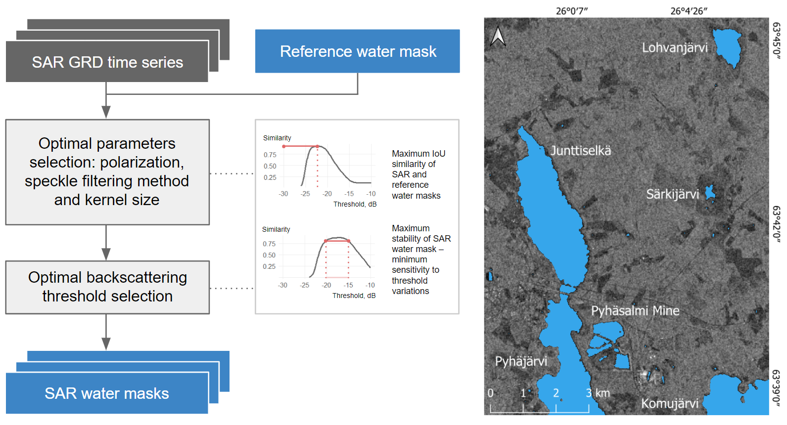
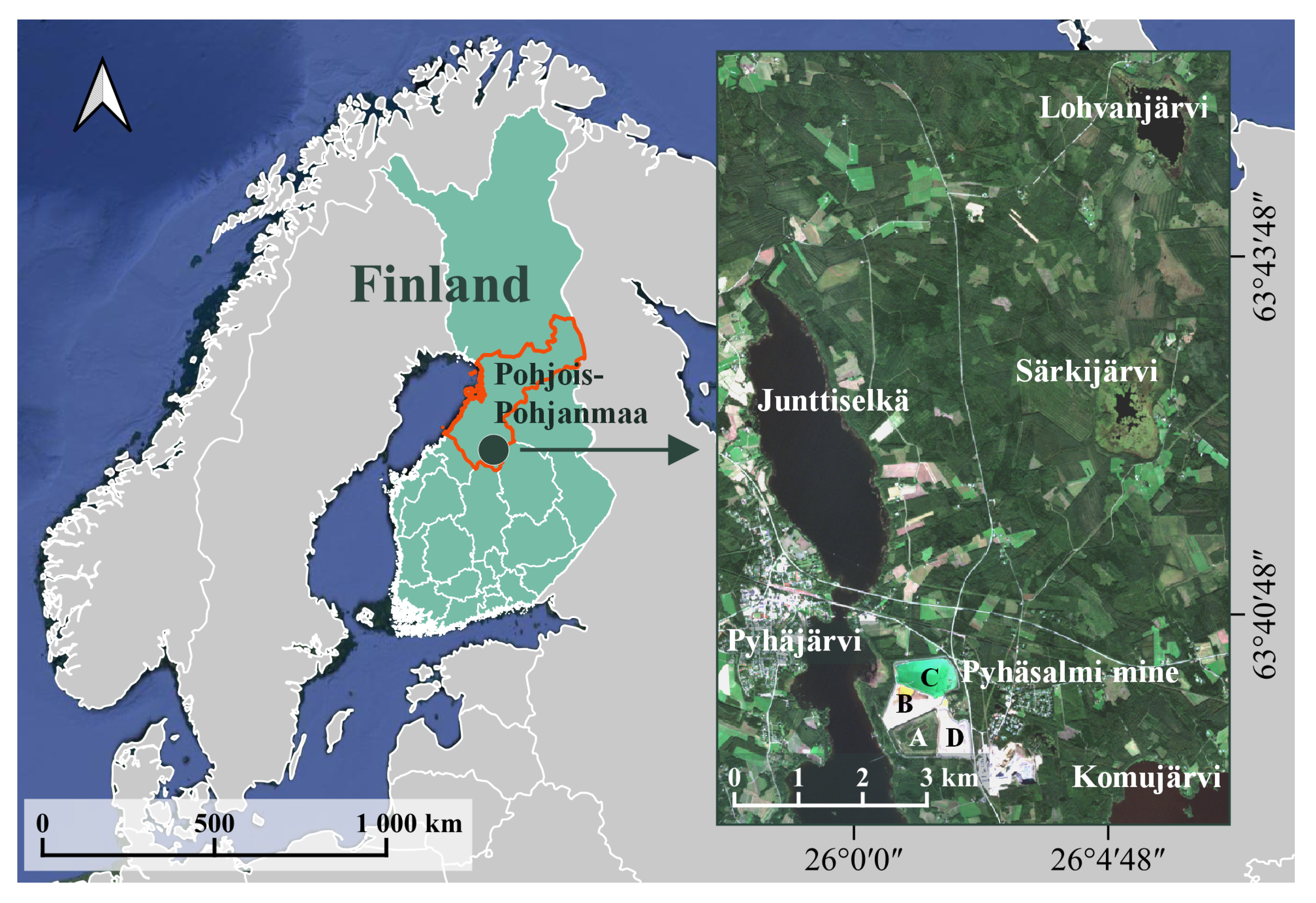
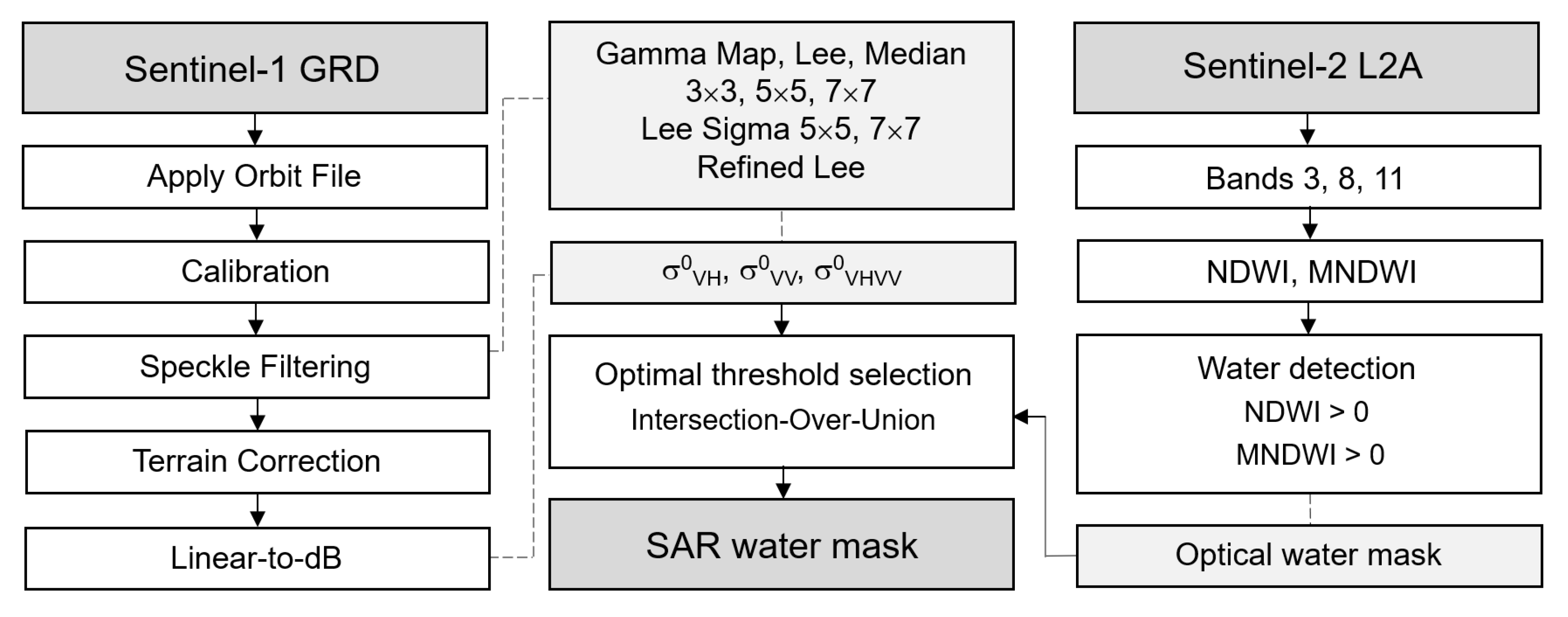
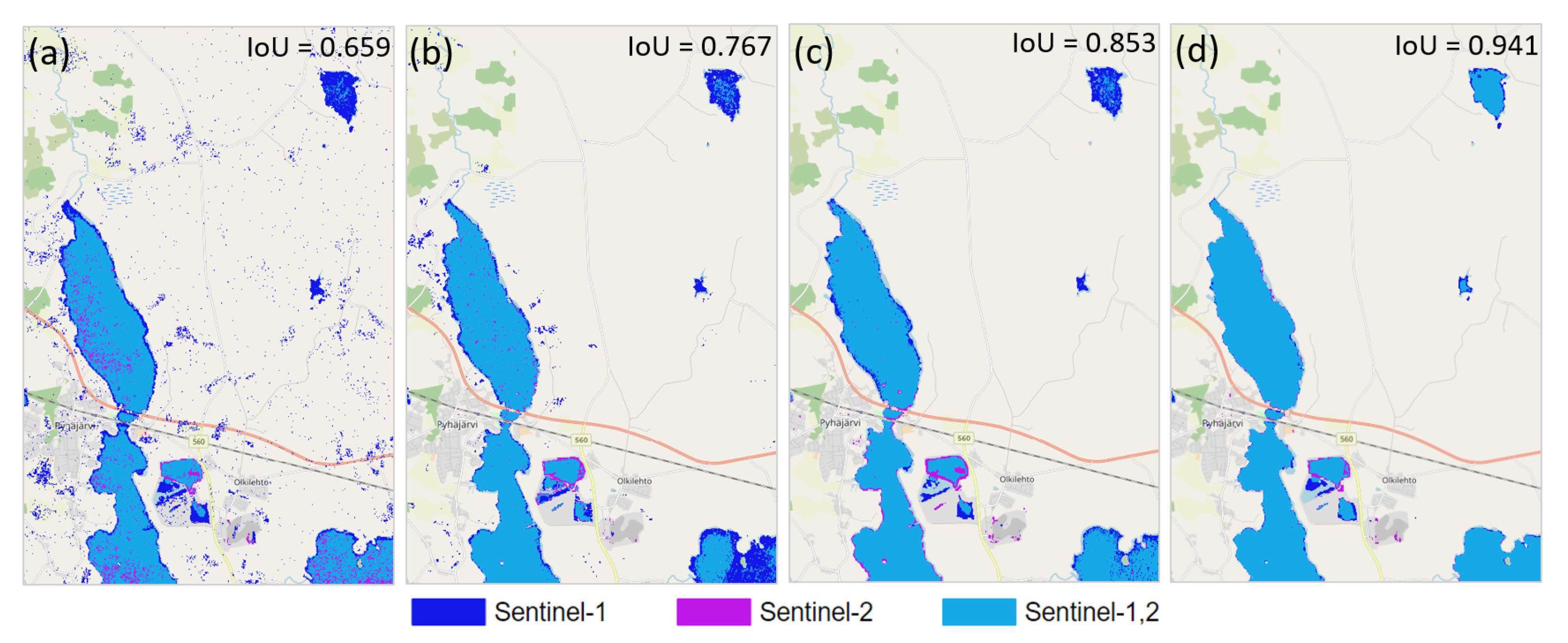
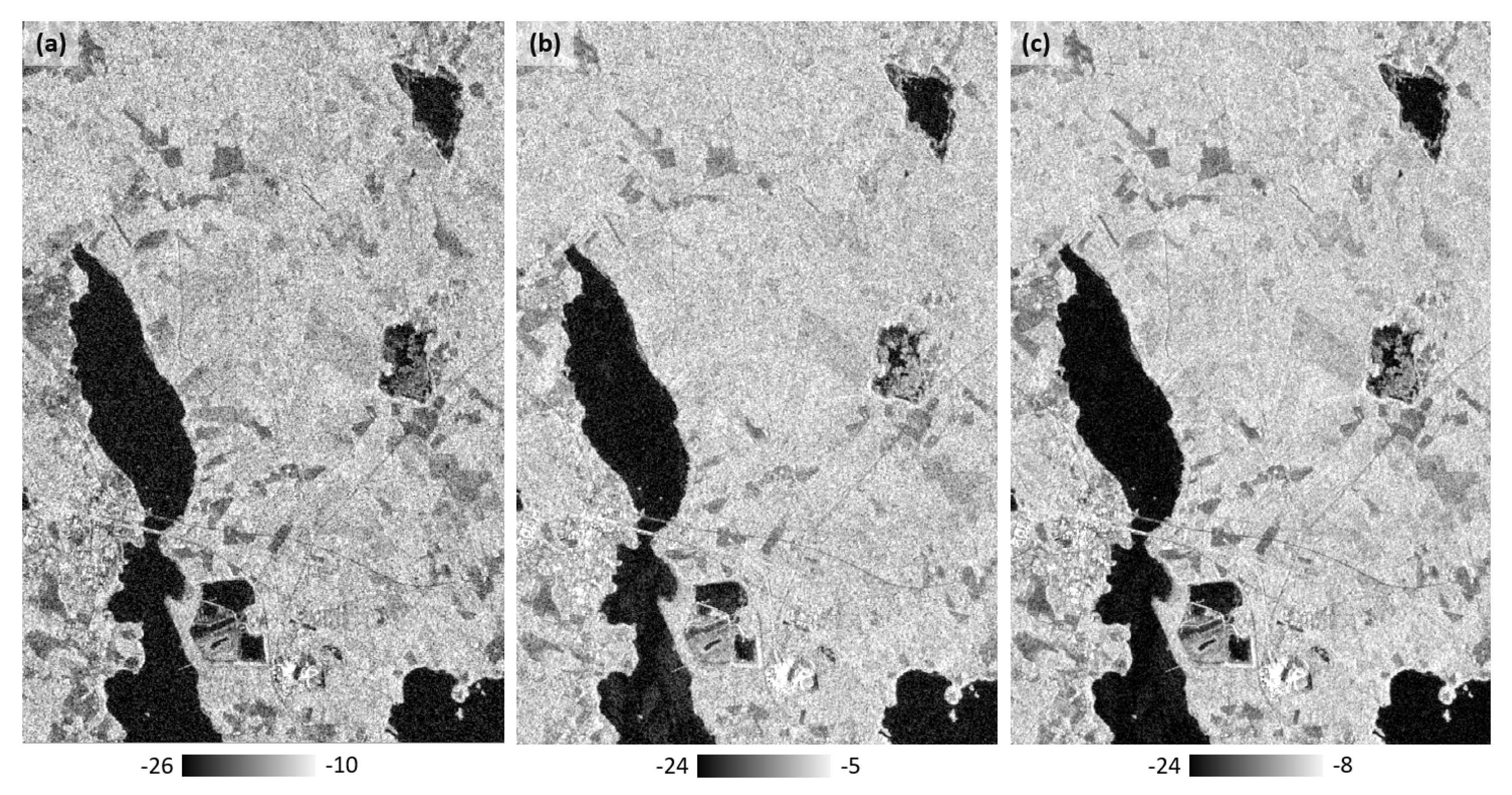
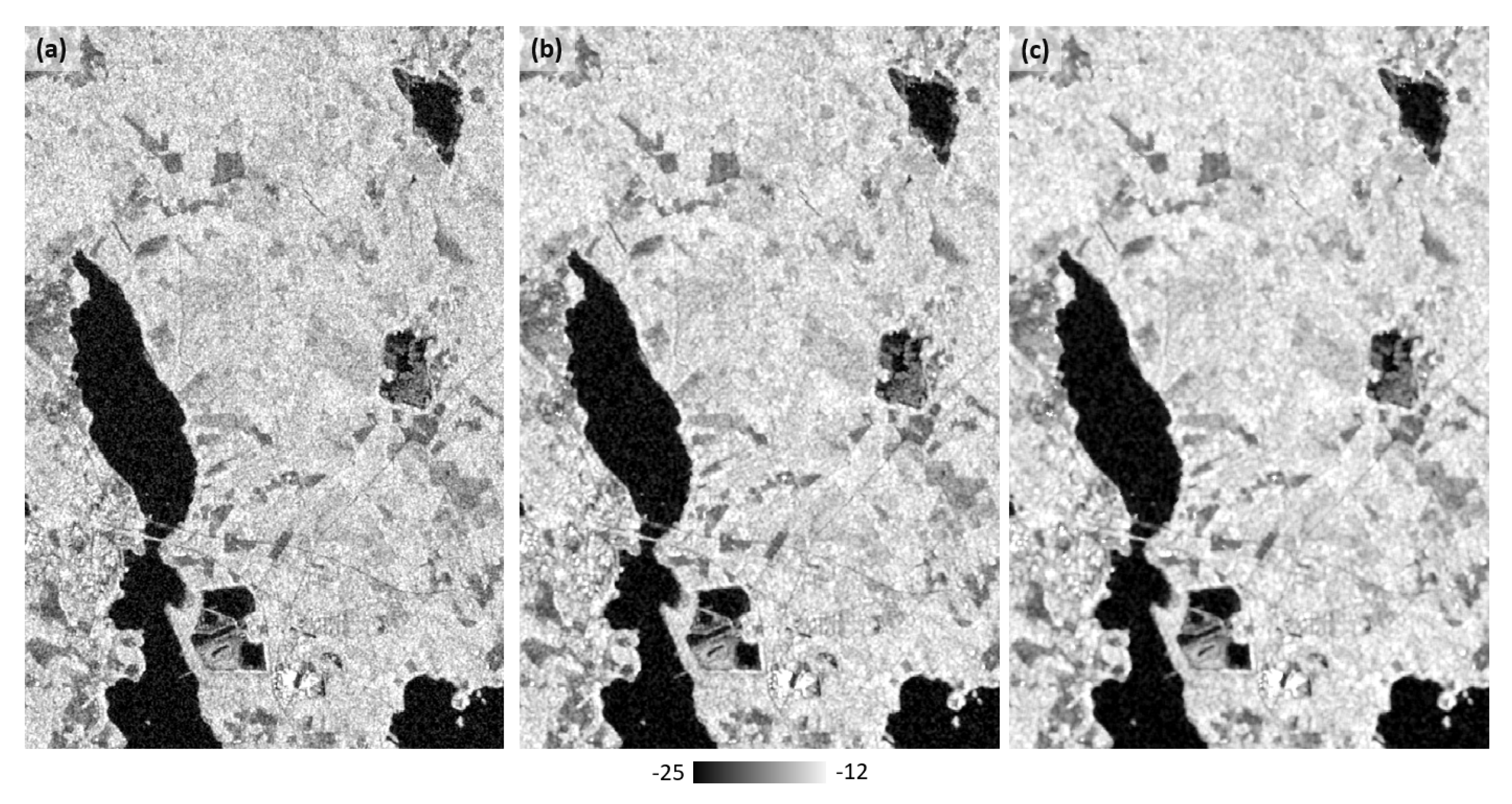
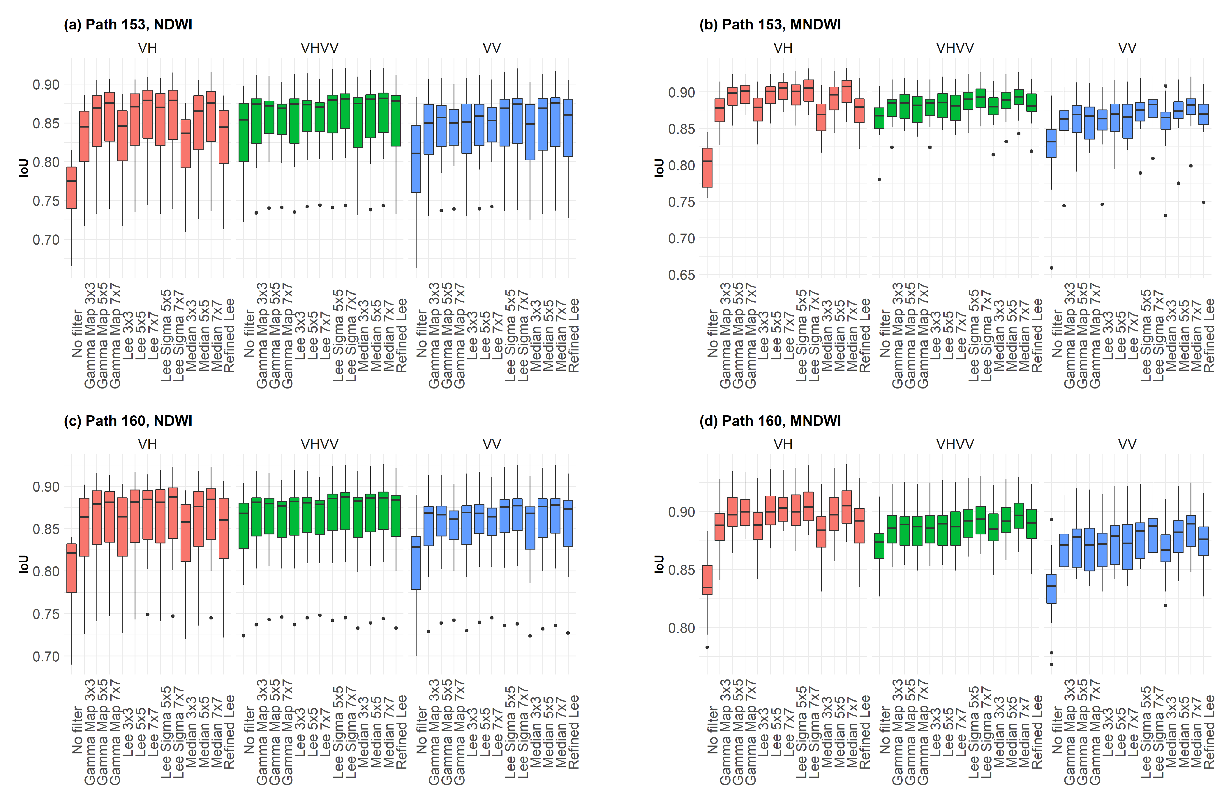
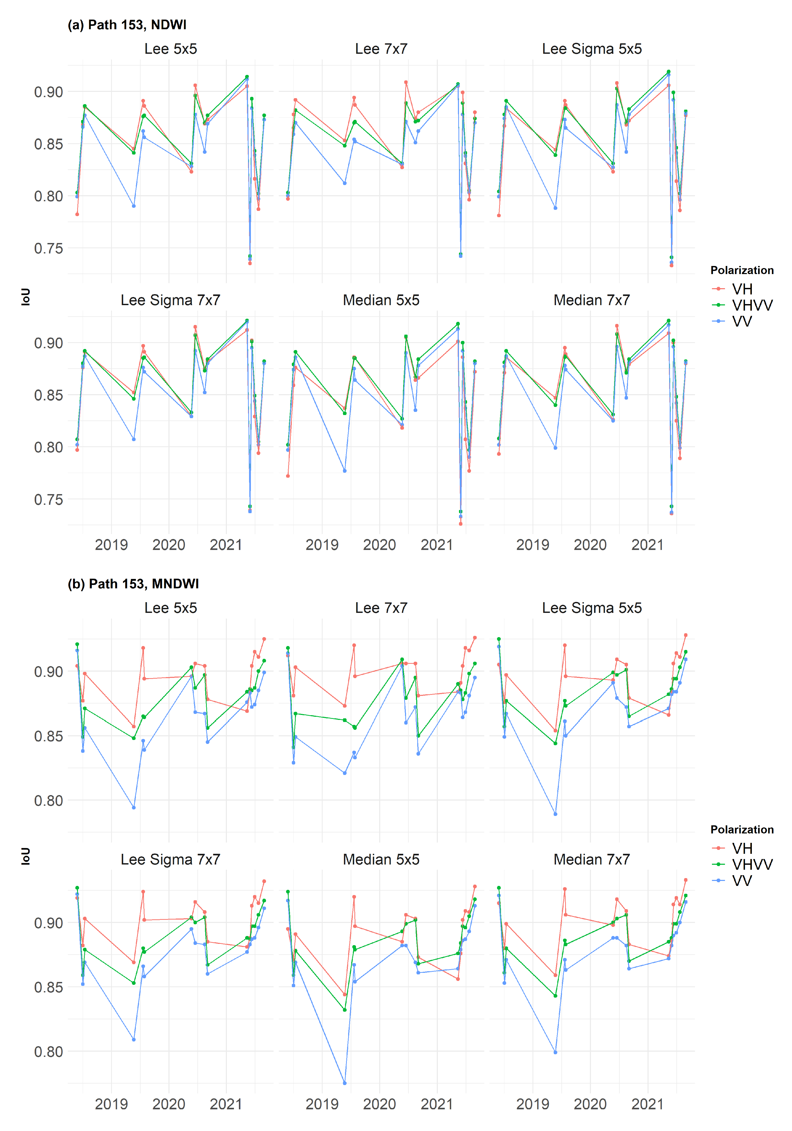
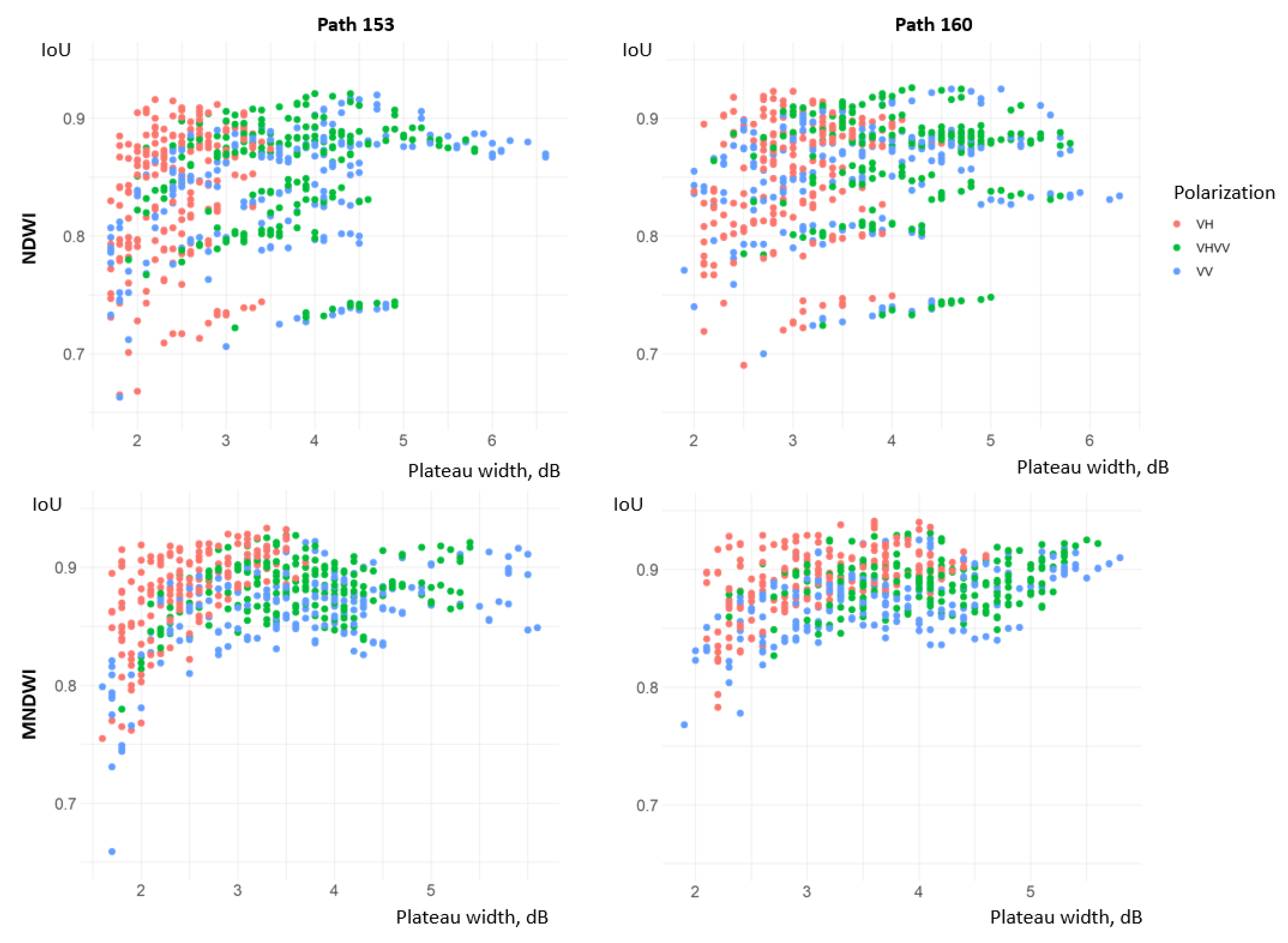
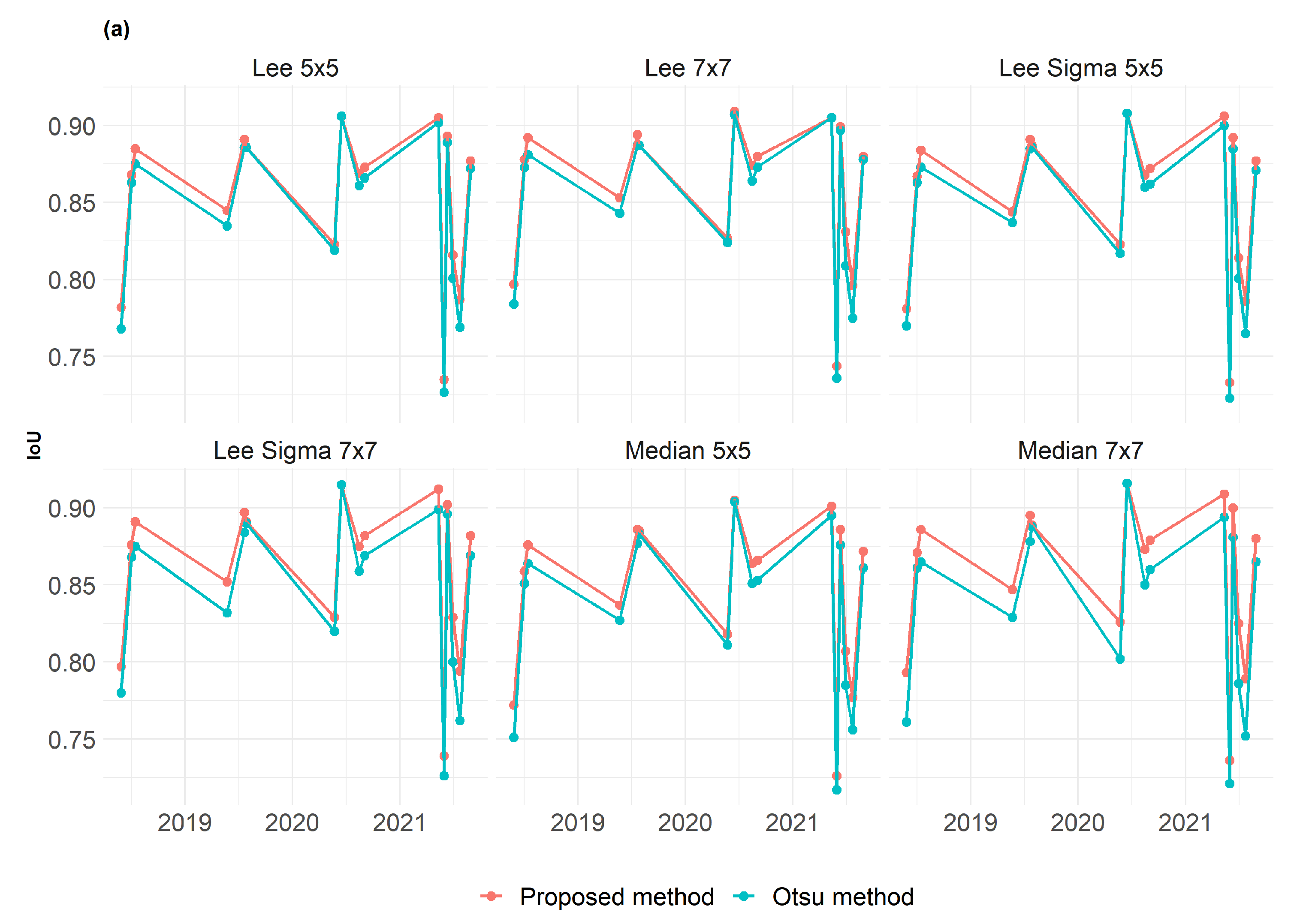
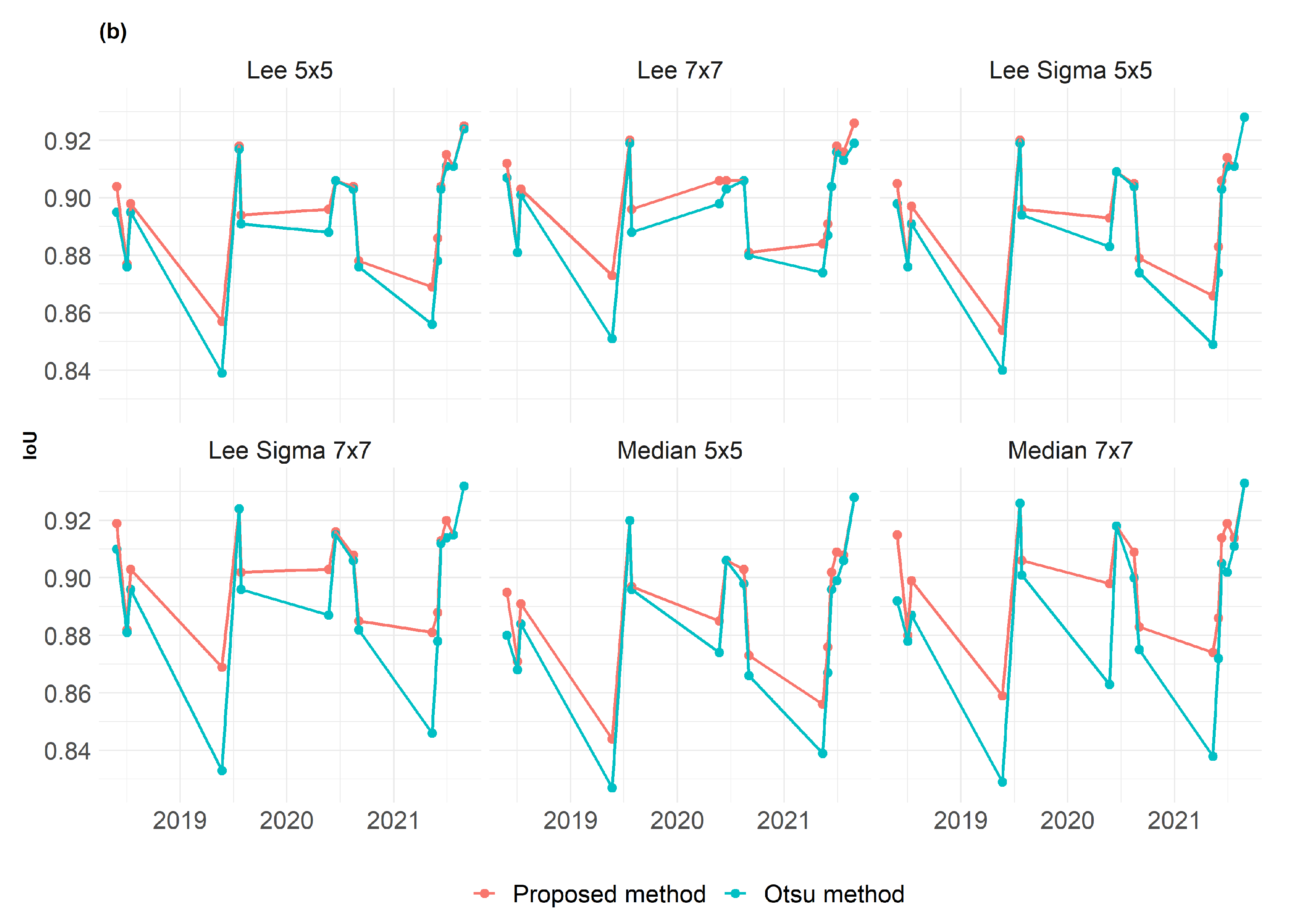
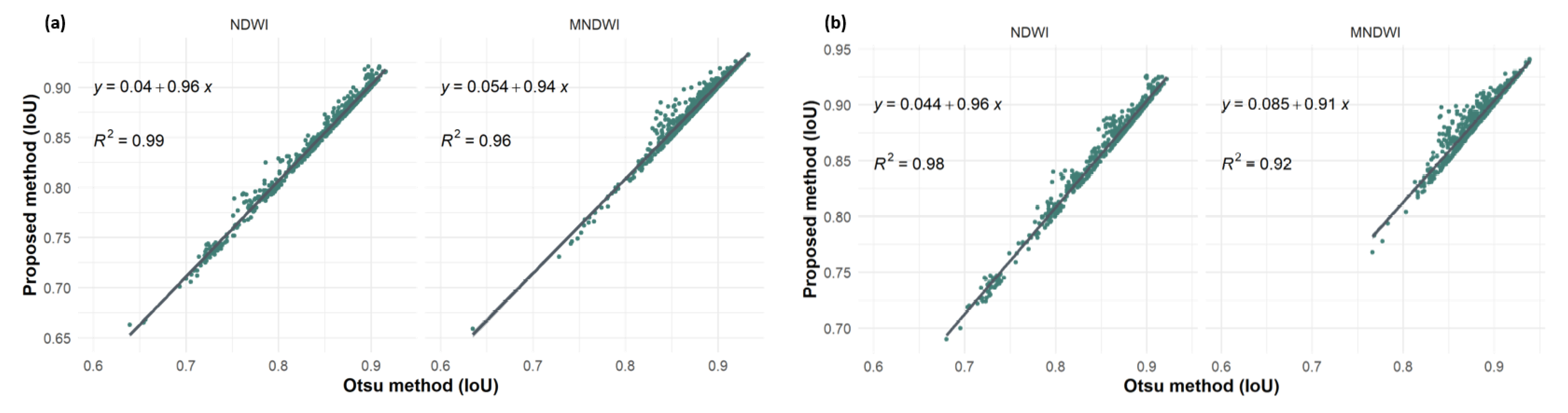
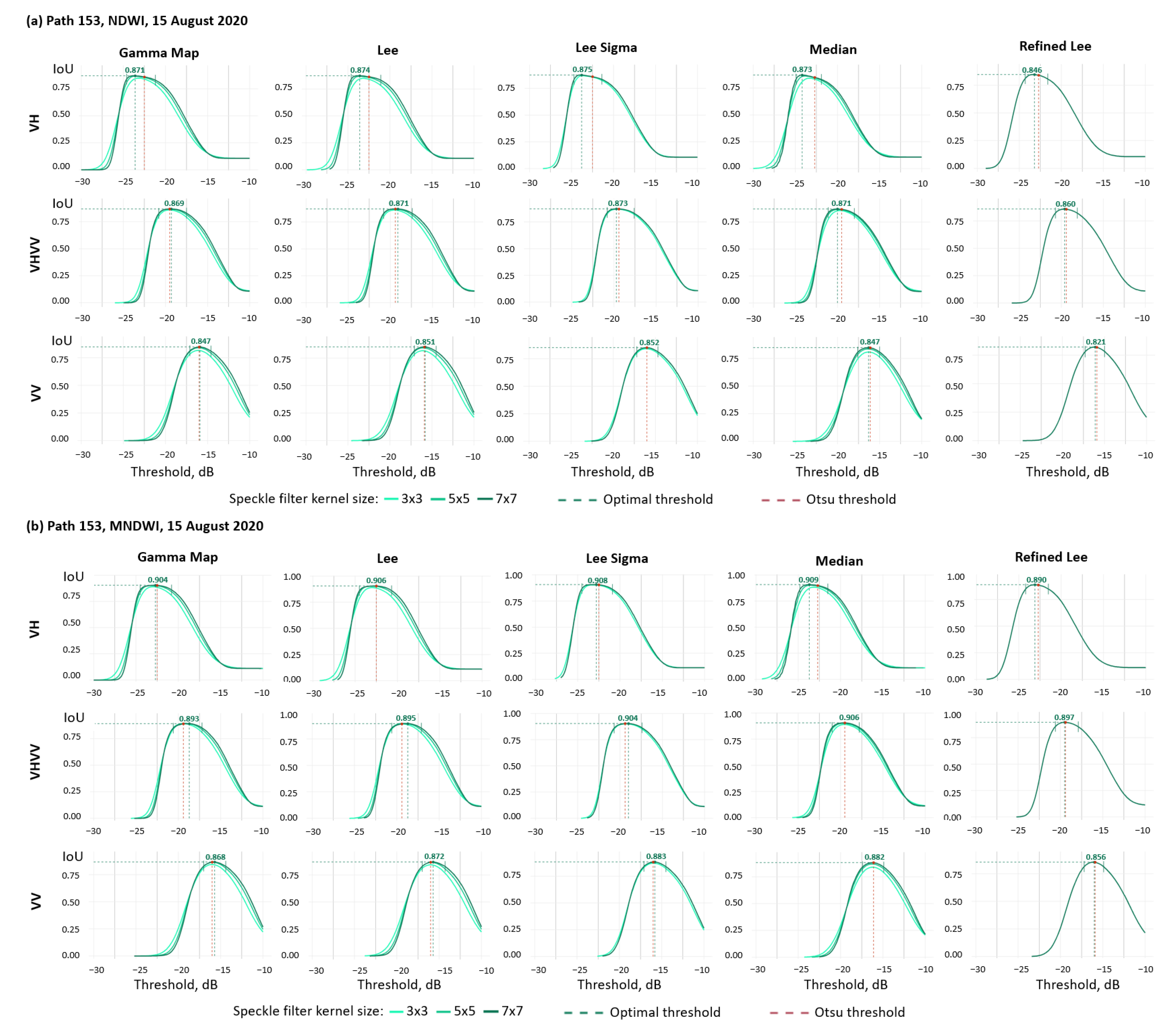
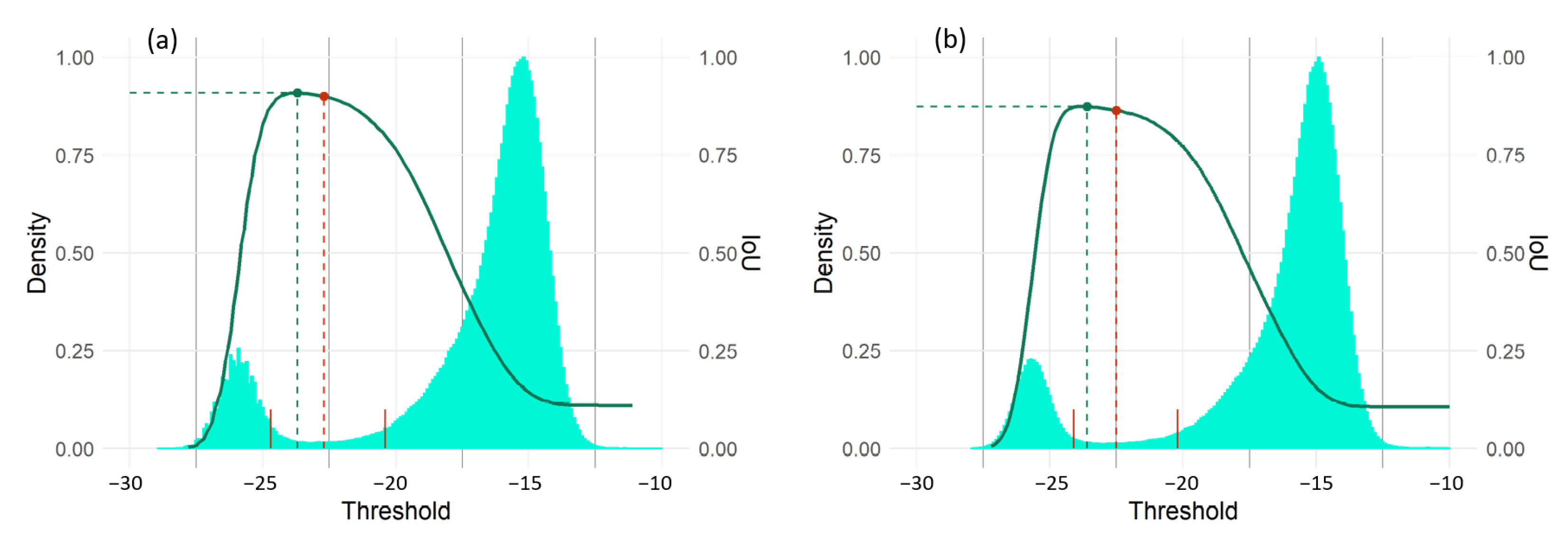
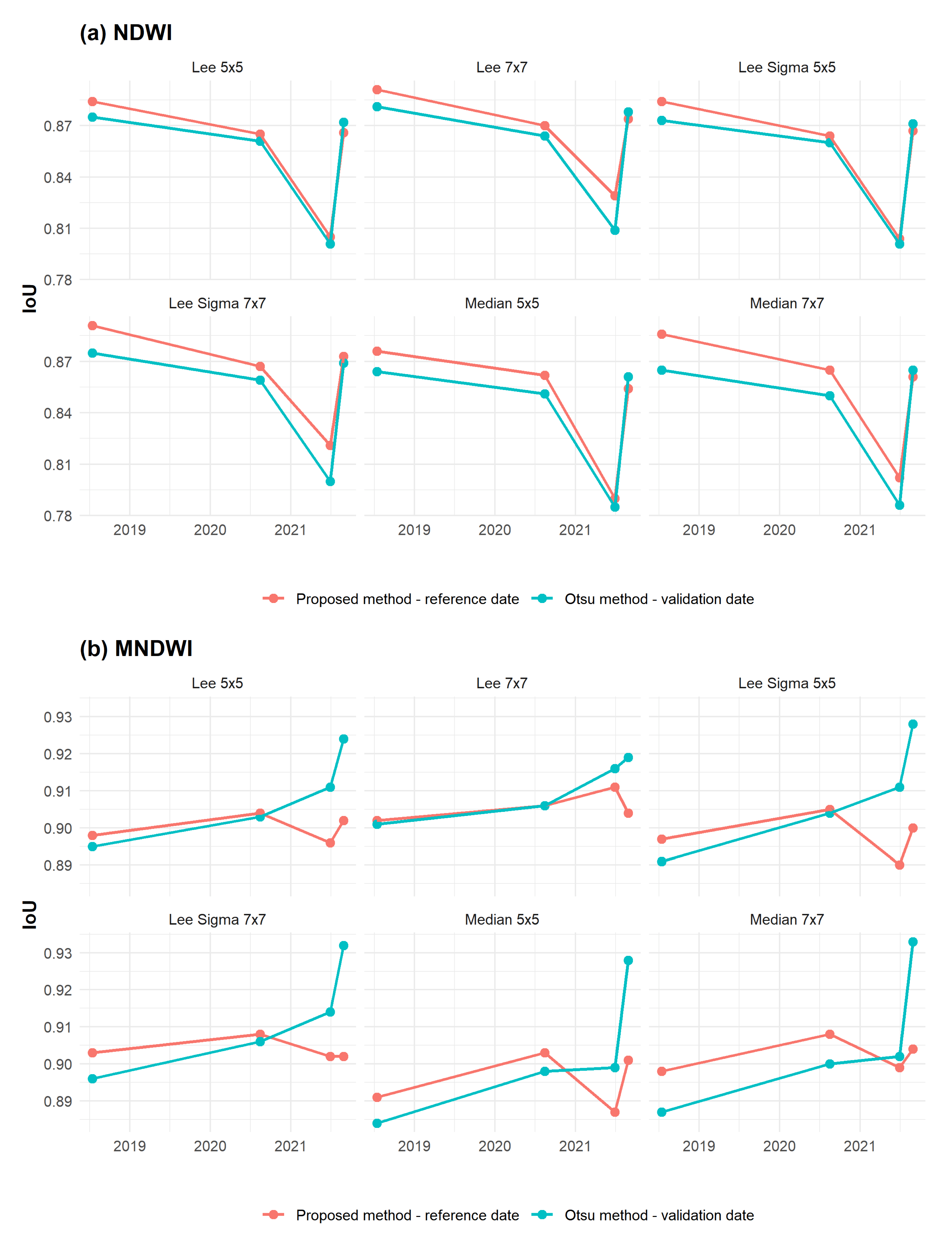
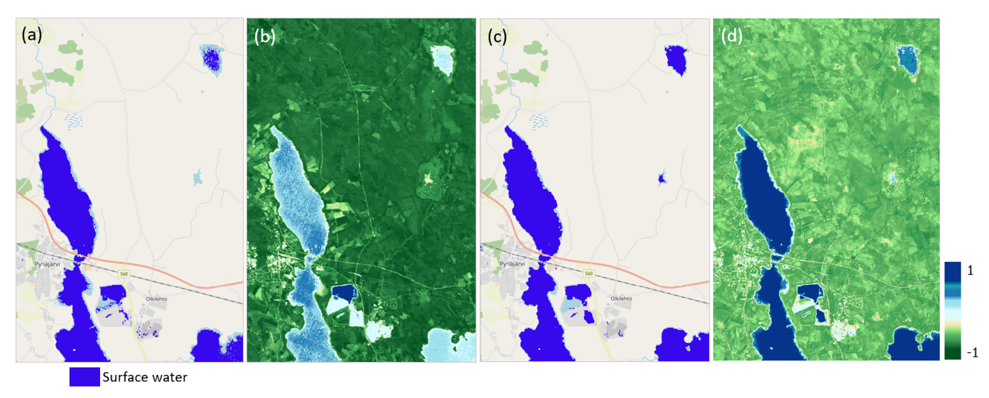
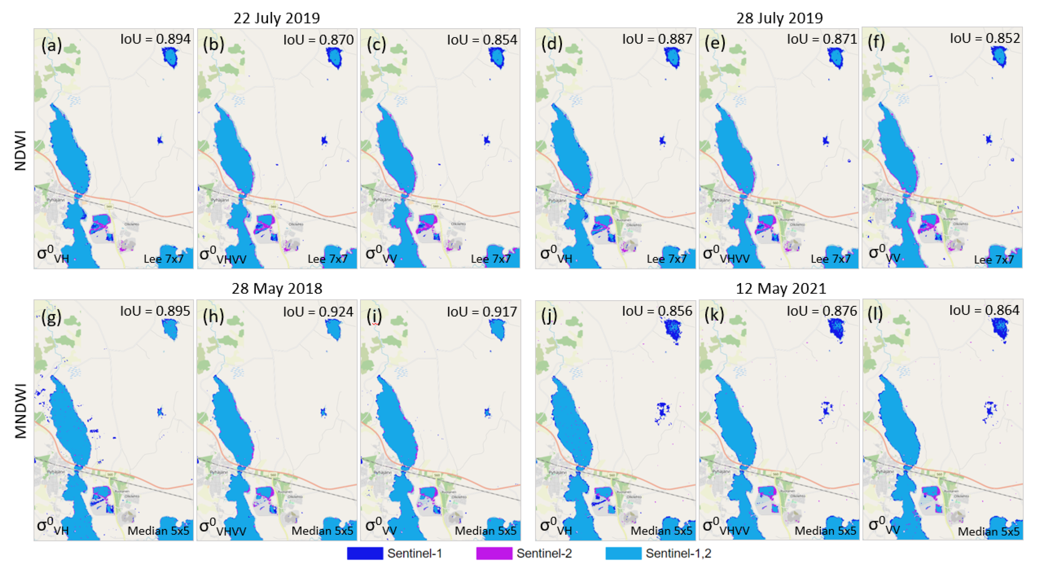
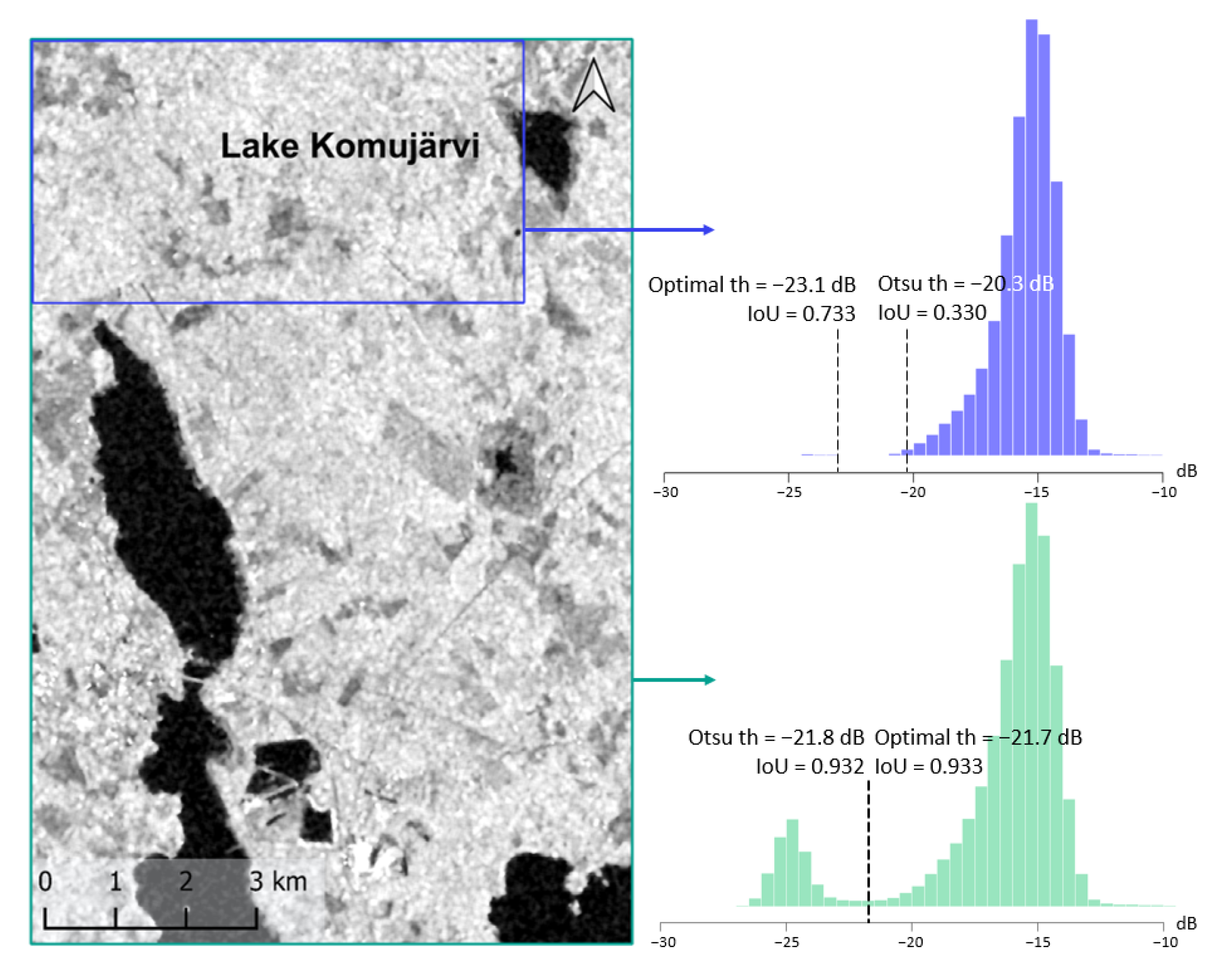
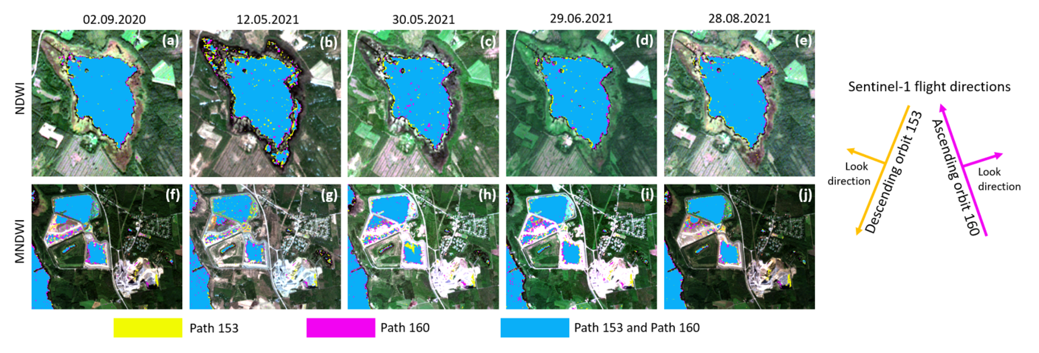
Table 1.
Sentinel-1 and Sentinel-2 images acquisition dates and time.
| Sentinel-1 | Sentinel-2 | |||
|---|---|---|---|---|
| Date | Time | Date | Time | |
| Path 153 | Path 160 | |||
| 28 August 2021 | 04:41:12 | 15:57:48 | 28 August 2021 | 10:02:50 |
| 23 July 2021 | 04:41:10 | 15:57:46 | 26 July 2021 | 09:52:55 |
| 29 June 2021 | 04:41:09 | 15:57:45 | 29 June 2021 | 10:02:50 |
| 11 June 2021 | 04:40:30 | 15:57:11 | 11 June 2021 | 09:52:53 |
| 30 May 2021 | 04:40:22 | 15:57:10 | 30 May 2021 | 10:02:49 |
| 12 May 2021 | 04:41:06 | 15:57:42 | 12 May 2021 | 09:52:50 |
| 02 September 2020 | 04:41:07 | 15:57:43 | 02 September 2020 | 10:02:53 |
| 15 August 2020 | 04:40:21 | 15:57:09 | 15 August 2020 | 09:52:55 |
| 16 June 2020 | 04:40:16 | 15:57:05 | 14 June 2020 | 10:02:55 |
| 23 May 2020 | 04:40:16 | 15:57:04 | 22 May 2020 | 09:52:57 |
| 28 July 2019 | 04:40:13 | 15:57:01 | 25 July 2019 | 10:02:57 |
| 22 July 2019 | 04:40:56 | 15:57:33 | 25 July 2019 | 10:02:57 |
| 23 May 2019 | 04:40:54 | 15:57:29 | 18 May 2019 | 09:52:55 |
| 15 July 2018 | 04:40:51 | 15:57:26 | 12 July 2018 | 09:50:30 |
| 03 July 2018 | 04:40:50 | 15:57:25 | 02 July 2018 | 09:50:30 |
| 28 May 2018 | 04:40:48 | 15:57:23 | 31 May 2018 | 10:00:23 |
Table 2.
Tables of median IoU similarity values for all combinations of speckle filtering parameters.
Table 2.
Tables of median IoU similarity values for all combinations of speckle filtering parameters.
| Path 153 | |||||||||||
|---|---|---|---|---|---|---|---|---|---|---|---|
| NDWI | MNDWI | ||||||||||
| Sf 1 | IoU | Sf | IoU | Sf | IoU | Sf | IoU | Sf | IoU | Sf | IoU |
| L7 2 | 0.879 | M7 3 | 0.876 | M7 | 0.882 | M7 | 0.908 | LS7 4 | 0.883 | M7 | 0.894 |
| LS7 | 0.879 | LS7 | 0.874 | LS7 | 0.881 | LS7 | 0.906 | M7 | 0.882 | LS7 | 0.893 |
| GM7 5 | 0.876 | LS5 | 0.869 | M5 | 0.881 | L7 | 0.905 | LS5 | 0.876 | LS5 | 0.890 |
| M7 | 0.876 | M5 | 0.869 | LS5 | 0.880 | GM7 | 0.902 | M5 | 0.874 | M5 | 0.889 |
| L5 | 0.871 | RL 6 | 0.861 | RL | 0.878 | L5 | 0.901 | L5 | 0.870 | L5 | 0.886 |
| LS5 | 0.870 | L5 | 0.859 | M3 | 0.875 | LS5 | 0.901 | RL | 0.870 | L3 | 0.885 |
| GM5 | 0.870 | GM5 | 0.857 | L3 | 0.875 | GM5 | 0.899 | GM5 | 0.869 | GM3 | 0.885 |
| M5 | 0.865 | L7 | 0.853 | GM3 | 0.874 | M5 | 0.896 | GM7 | 0.867 | GM5 | 0.885 |
| L3 | 0.846 | L3 | 0.851 | L5 | 0.874 | RL | 0.880 | L7 | 0.866 | GM7 | 0.882 |
| GM3 | 0.845 | GM3 | 0.850 | GM5 | 0.872 | L3 | 0.879 | M3 | 0.865 | L7 | 0.881 |
| RL | 0.845 | GM7 | 0.850 | L7 | 0.871 | GM3 | 0.878 | L3 | 0.864 | RL | 0.881 |
| M3 | 0.837 | M3 | 0.849 | GM7 | 0.869 | M3 | 0.869 | GM3 | 0.863 | M3 | 0.880 |
| None | 0.775 | None | 0.811 | None | 0.854 | None | 0.805 | None | 0.832 | None | 0.868 |
| SD 7 | 0.029 | SD | 0.017 | SD | 0.007 | SD | 0.028 | SD | 0.013 | SD | 0.007 |
| LS7 | 0.887 | M7 | 0.878 | LS7 | 0.887 | M7 | 0.905 | M7 | 0.890 | M7 | 0.897 |
| L7 | 0.885 | LS7 | 0.877 | M7 | 0.887 | LS7 | 0.904 | LS7 | 0.888 | LS7 | 0.894 |
| M7 | 0.885 | M5 | 0.876 | M5 | 0.886 | L7 | 0.903 | LS5 | 0.883 | LS5 | 0.892 |
| L5 | 0.882 | LS5 | 0.876 | LS5 | 0.886 | GM7 | 0.900 | M5 | 0.882 | M5 | 0.892 |
| GM7 | 0.881 | RL | 0.874 | RL | 0.884 | L5 | 0.900 | L5 | 0.879 | RL | 0.890 |
| LS5 | 0.881 | L3 | 0.869 | M3 | 0.883 | LS5 | 0.900 | GM5 | 0.878 | L5 | 0.890 |
| GM5 | 0.879 | GM3 | 0.869 | L3 | 0.882 | GM5 | 0.898 | RL | 0.876 | GM5 | 0.889 |
| M5 | 0.876 | L5 | 0.868 | GM3 | 0.881 | M5 | 0.898 | L7 | 0.873 | GM7 | 0.887 |
| L3 | 0.864 | M3 | 0.868 | L5 | 0.881 | RL | 0.892 | L3 | 0.872 | L7 | 0.887 |
| GM3 | 0.864 | GM5 | 0.867 | GM5 | 0.880 | L3 | 0.889 | GM3 | 0.871 | GM3 | 0.886 |
| RL | 0.860 | L7 | 0.864 | L7 | 0.879 | GM3 | 0.888 | GM7 | 0.871 | L3 | 0.886 |
| M3 | 0.858 | GM7 | 0.861 | GM7 | 0.877 | M3 | 0.884 | M3 | 0.867 | M3 | 0.885 |
| None | 0.821 | None | 0.828 | None | 0.868 | None | 0.835 | None | 0.836 | None | 0.874 |
| SD | 0.018 | SD | 0.013 | SD | 0.005 | SD | 0.018 | SD | 0.013 | SD | 0.006 |
Notes: 1 Sf—Speckle filter; 2 L3—Lee 3 × 3, L5—Lee 5 × 5, L7—Lee 7 × 7; 3 M3—Median 3 × 3, M5—Median 5 × 5, M7—Median 7 × 7; 4 LS5—Lee Sigma 5 × 5, LS7—Lee Sigma 7 × 7; 5 GM3—Gamma Map 3 × 3, GM5—Gamma; p 5 × 5, GM7—Gamma Map 7 × 7; 6 RL—Refined Lee; and 7 SD—standard deviation of the median IoU.
Table 3.
Quantitative plateau characteristics for all filters, polarization, and reference masks, 22 July 2019.
Table 3.
Quantitative plateau characteristics for all filters, polarization, and reference masks, 22 July 2019.
| NDWI | MNDWI | ||||||||||
|---|---|---|---|---|---|---|---|---|---|---|---|
| Filter | Start 1 | End 2 | PW 3 | IoU | Filter | Start | End | PW | IoU | ||
| L7 4 | −14.8 | −19.3 | 4.5 | 0.854 | GM7 5 | −14.8 | −19.2 | 4.4 | 0.836 | ||
| GM7 | −14.9 | −19.3 | 4.4 | 0.852 | L7 | −14.7 | −19.1 | 4.4 | 0.837 | ||
| LS7 6 | −15.0 | −19.4 | 4.4 | 0.876 | LS7 | −14.9 | −19.2 | 4.3 | 0.866 | ||
| GM7 | −17.1 | −21.5 | 4.4 | 0.869 | GM5 | −15.1 | −19.3 | 4.2 | 0.845 | ||
| L7 | −17.1 | −21.5 | 4.4 | 0.870 | M7 7 | −15.3 | −19.5 | 4.2 | 0.871 | ||
| LS7 | −17.3 | −21.7 | 4.4 | 0.885 | GM7 | −17.0 | −21.2 | 4.2 | 0.857 | ||
| M7 | −15.4 | −19.7 | 4.3 | 0.878 | L5 | −15.1 | −19.2 | 4.1 | 0.846 | ||
| M7 | −17.7 | −22.0 | 4.3 | 0.886 | LS5 | −15.1 | −19.2 | 4.1 | 0.861 | ||
| GM5 | −15.2 | −19.4 | 4.2 | 0.860 | GM5 | −17.3 | −21.4 | 4.1 | 0.864 | ||
| L5 | −15.2 | −19.4 | 4.2 | 0.862 | M7 | −17.5 | −21.6 | 4.1 | 0.886 | ||
| GM5 | −17.4 | −21.6 | 4.2 | 0.875 | L5 | −17.3 | −21.4 | 4.1 | 0.865 | ||
| L5 | −17.4 | −21.6 | 4.2 | 0.876 | L7 | −17.0 | −21.1 | 4.1 | 0.857 | ||
| LS5 | −17.5 | −21.7 | 4.2 | 0.884 | LS7 | −17.2 | −21.3 | 4.1 | 0.880 | ||
| LS5 | −15.3 | −19.4 | 4.1 | 0.873 | M5 | −15.5 | −19.5 | 4.0 | 0.867 | ||
| M5 | −17.9 | −21.9 | 4.0 | 0.885 | M5 | −17.7 | −21.7 | 4.0 | 0.881 | ||
| M5 | −15.7 | −19.6 | 3.9 | 0.875 | LS5 | −17.4 | −21.4 | 4.0 | 0.877 | ||
| RL 8 | −15.7 | −19.5 | 3.8 | 0.874 | RL | −17.7 | −21.5 | 3.8 | 0.880 | ||
| RL | −17.9 | −21.7 | 3.8 | 0.884 | RL | −15.6 | −19.3 | 3.7 | 0.865 | ||
| GM3 | −15.7 | −19.3 | 3.6 | 0.864 | GM3 | −17.7 | −21.4 | 3.7 | 0.869 | ||
| L3 | −15.7 | −19.3 | 3.6 | 0.865 | L3 | −17.7 | −21.4 | 3.7 | 0.870 | ||
| GM3 | −17.9 | −21.5 | 3.6 | 0.878 | GM3 | −15.6 | −19.2 | 3.6 | 0.852 | ||
| L3 | −17.9 | −21.5 | 3.6 | 0.879 | L3 | −15.6 | −19.2 | 3.6 | 0.852 | ||
| M3 | −16.0 | −19.5 | 3.5 | 0.867 | M3 | −15.9 | −19.4 | 3.5 | 0.857 | ||
| M3 | −18.2 | −21.7 | 3.5 | 0.881 | M3 | −18.0 | −21.5 | 3.5 | 0.876 | ||
| L7 | −20.6 | −23.8 | 3.2 | 0.894 | GM7 | −20.2 | −23.3 | 3.1 | 0.919 | ||
| G7 | −20.7 | −23.8 | 3.1 | 0.892 | L7 | −20.2 | −23.3 | 3.1 | 0.920 | ||
| LS7 | −20.8 | −23.8 | 3.0 | 0.897 | LS7 | −20.3 | −23.4 | 3.1 | 0.924 | ||
| M7 | −20.7 | −23.7 | 3.0 | 0.926 | |||||||
Notes: 1 Start—Plateau upper bound; 2 End—Plateau lower bound; 3 PW—PlateauWidth; 4 L3—Lee 3 × 3, L5—Lee 5 × 5, L7—Lee 7 × 7; 5 GM3—Gamma Map 3 × 3, GM5—Gamma Map 5 × 5, GM7—Gamma Map 7 × 7; 6 LS5—Lee Sigma 5 × 5, LS7—Lee Sigma 7 × 7; 7 M3—Median 3 × 3, M5—Median 5 × 5, M7—Median 7 × 7; 8 RL—Refined Lee.
Table 4.
Comparison of the accuracy of SAR water masks generated by the Otsu method and the proposed method based on the optimal thresholds of the reference date and the averaged optimal thresholds for all dates in 2018–2020.
Table 4.
Comparison of the accuracy of SAR water masks generated by the Otsu method and the proposed method based on the optimal thresholds of the reference date and the averaged optimal thresholds for all dates in 2018–2020.
| 29 June 2021 1 | Otsu IoU | Reference Date—11 June 2021 | All Dates 2018–2020 | ||||
|---|---|---|---|---|---|---|---|
| Th 2 | Opt. IoU 3 | IoU 4 | Th | Opt. IoU | IoU | ||
| Lee 5 × 5 | 0.911 | −22.5 | 0.896 | 0.015 | −22.7 | 0.913 | −0.002 |
| Lee 7 × 7 | 0.916 | −22.2 | 0.911 | 0.005 | −22.5 | 0.917 | −0.001 |
| Lee Sigma 5 × 5 | 0.911 | −22.4 | 0.890 | 0.021 | −22.7 | 0.914 | −0.003 |
| Lee Sigma 7 × 7 | 0.914 | −22.4 | 0.902 | 0.012 | −22.7 | 0.920 | −0.006 |
| Median 5 × 5 | 0.899 | −22.7 | 0.887 | 0.012 | −23.0 | 0.908 | −0.009 |
| Median 7 × 7 | 0.902 | −23.0 | 0.899 | 0.003 | −23.1 | 0.919 | −0.017 |
| 28 August 2021 | OtsuIoU | Reference Date—11 June 2021 | All Dates 2018–2020 | ||||
| Th | Opt.IoU | IoU | Th | Opt.IoU | IoU | ||
| Lee 5 × 5 | 0.924 | −22.2 | 0.902 | 0.022 | −22.7 | 0.918 | 0.006 |
| Lee 7 × 7 | 0.919 | −22.3 | 0.904 | 0.015 | −22.5 | 0.915 | 0.004 |
| Lee Sigma 5 × 5 | 0.928 | −22.2 | 0.900 | 0.028 | −22.7 | 0.922 | 0.006 |
| Lee Sigma 7 × 7 | 0.932 | −21.8 | 0.902 | 0.030 | −22.7 | 0.923 | 0.009 |
| Median 5 × 5 | 0.928 | −22.3 | 0.901 | 0.027 | −22.7 | 0.922 | 0.006 |
| Median 7 × 7 | 0.933 | −22.3 | 0.904 | 0.029 | −23.1 | 0.926 | 0.007 |
Notes: 1 Validation date; 2 Th—Threshold (dB); 3 Opt. IoU—Optimal IoU; 4 D IoU—IoU difference Otsu, optimal.
Table 5.
threshold values and IoU metrics of SAR and optical water masks similarity for path = 160, path = 153, and all observation dates.
Table 5.
threshold values and IoU metrics of SAR and optical water masks similarity for path = 160, path = 153, and all observation dates.
| SAR Date | NDWI | MNDWI | ||||||
|---|---|---|---|---|---|---|---|---|
| Similarity (IoU) | Threshold (dB) | Similarity (IoU) | Threshold (dB) | |||||
| 153 1 | 160 1 | 153 | 160 | 153 | 160 | 153 | 160 | |
| 28 August 2021 | 0.880 | 0.884 | −22.7 | −24.6 | 0.926 | 0.936 | −21.3 | −22.7 |
| 23 July 2021 | 0.796 | 0.802 | −23.1 | −24.1 | 0.916 | 0.900 | −21.2 | −21.8 |
| 29 June 2021 | 0.831 | 0.841 | −23.1 | −23.9 | 0.918 | 0.907 | −22.2 | −22.2 |
| 11 June 2021 | 0.899 | 0.901 | −23.4 | −23.7 | 0.904 | 0.895 | −23.0 | −23.1 |
| 30 May 2021 | 0.744 | 0.749 | −23.9 | −24.8 | 0.891 | 0.892 | −23.6 | −24.0 |
| 12 May 2021 | 0.905 | 0.907 | −22.1 | −23.2 | 0.884 | 0.891 | −22.7 | −23.9 |
| 02 September 2020 | 0.880 | 0.885 | −23.2 | −24.3 | 0.881 | 0.883 | −22.7 | −23.3 |
| 15 August 2020 | 0.874 | 0.879 | −23.6 | −24.6 | 0.906 | 0.912 | −22.5 | −23.3 |
| 16 June 2020 | 0.909 | 0.914 | −23.0 | −23.7 | 0.906 | 0.912 | −22.9 | −23.5 |
| 23 May 2020 | 0.827 | 0.827 | −23.2 | −24.2 | 0.906 | 0.910 | −23.5 | −24.4 |
| 28 July 2019 | 0.887 | 0.894 | −22.6 | −23.1 | 0.896 | 0.906 | −22.1 | −22.4 |
| 22 July 2019 | 0.894 | 0.899 | −22.5 | −23.4 | 0.920 | 0.922 | −21.6 | −21.5 |
| 23 May 2019 | 0.853 | 0.858 | −23.2 | −24.7 | 0.873 | 0.883 | −23.3 | −24.8 |
| 15 July 2018 | 0.892 | 0.893 | −24.2 | −23.2 | 0.903 | 0.898 | −22.0 | −22.4 |
| 03 July 2018 | 0.878 | 0.887 | −22.7 | −24.0 | 0.881 | 0.885 | −21.8 | −22.8 |
| 28 May 2018 | 0.797 | 0.811 | −23.2 | −24.0 | 0.912 | 0.924 | −22.9 | −23.6 |
Note: 1 153—Path 153, 160—Path 160.
Publisher’s Note: MDPI stays neutral with regard to jurisdictional claims in published maps and institutional affiliations. |
© 2022 by the authors. Licensee MDPI, Basel, Switzerland. This article is an open access article distributed under the terms and conditions of the Creative Commons Attribution (CC BY) license (https://creativecommons.org/licenses/by/4.0/).
Share and Cite
MDPI and ACS Style
Kavats, O.; Khramov, D.; Sergieieva, K. Surface Water Mapping from SAR Images Using Optimal Threshold Selection Method and Reference Water Mask. Water 2022, 14, 4030. https://doi.org/10.3390/w14244030
AMA Style
Kavats O, Khramov D, Sergieieva K. Surface Water Mapping from SAR Images Using Optimal Threshold Selection Method and Reference Water Mask. Water. 2022; 14(24):4030. https://doi.org/10.3390/w14244030
Chicago/Turabian StyleKavats, Olena, Dmitriy Khramov, and Kateryna Sergieieva. 2022. "Surface Water Mapping from SAR Images Using Optimal Threshold Selection Method and Reference Water Mask" Water 14, no. 24: 4030. https://doi.org/10.3390/w14244030
Note that from the first issue of 2016, this journal uses article numbers instead of page numbers. See further details here.